Abstract

The physical phase space in gauge systems is studied. Effects caused by a non-Euclidean geometry of the physical phase space in quantum gauge models are described in the operator and path integral formalisms. The projection on the Dirac gauge invariant states is used to derive a necessary modification of the Hamiltonian path integral in gauge theories of the Yang-Mills type with fermions that takes into account the non-Euclidean geometry of the physical phase space. The new path integral is applied to resolve the Gribov obstruction. Applications to the Kogut-Susskind lattice gauge theory are given. The basic ideas are illustrated with examples accessible for non-specialists.

1 Introduction

Yang-Mills theory and gauge theories in general play the most profound role in our present understanding of the universe. Nature is quantum in its origin so any classical gauge model should be promoted to its quantum version in order to be used as a model of the physical reality. We usually do this by applying one or another quantization recipe which we believe to lead to a consistent quantum theory. In general, quantization is by no means unique and should be regarded as a theoretical way to guess the true theory. We certainly expect any quantization procedure to comply with some physical principles, like the correspondence principle, gauge invariance, etc. And finally, the resulting quantum theory should not have any internal contradiction. All these conditions are rather loose to give us a unique quantization recipe.

The simplest way to quantize a theory is to use canonical quantization based on the Hamiltonian formalism of the classical theory. Given a set of canonical coordinates and momenta, one promotes them into a set of self-adjoint operators satisfying the Heisenberg commutation relations. Any classical observable, as a function on the phase space, becomes a function of the canonical operators. Due to the noncommutativity of the canonical operators, there is no unique correspondence between classical and quantum observables. One can modify a quantum observable by adding some operators proportional to commutators of the canonical operators. This will not make any difference in the formal limit when the Planck constant, which “measures” the noncommutativity of the canonical variables, vanishes. In classical mechanics, the Hamiltonian equations of motion are covariant under general canonical transformations. So there is no preference of choosing a particular set of canonical variables to span the phase space of the system. It was, however, found in practice that canonical quantization would be successful only when applied with the phase space coordinates referring to a Cartesian system of axes and not to more general curvilinear coordinates [1]. On the other hand, a global Cartesian coordinate system can be found only if the phase space of the system is Euclidean. This comprises a fundamental restriction on the canonical quantization recipe.

Another quantization method is due to Feynman [2] which, at first sight, seems to avoid the use of noncommutative phase space variables. Given a classical action for a system in the Lagrangian form, which is usually assumed to be quadratic in velocities, the quantum mechanical transition amplitude between two fixed points of the configuration space is determined by a sum over all continuous paths connecting these points with weight being the phase exponential of the classical action divided by the Planck constant. Such a sum is called the Lagrangian path integral. If the action is taken in the Hamiltonian form, the sum is extended over all phase-space trajectories connecting the initial and final states of the system and, in addition, this sum also involves integration over the momenta of the final and initial states. Recall that a phase-space point specifies uniquely a state of a Hamiltonian system in classical theory. Such a sum is called the Hamiltonian path integral. One should however keep in mind that such a definition of the Hamiltonian path integral (as a sum over paths in a phase space) is formal. One usually defines it by a specific finite dimensional integral on the time lattice rather than a sum over paths in a phase space. The correspondence principle follows from the stationary phase approximation to the sum over paths when the classical action is much greater than the Planck constant. The stationary point, if any, of the action is a classical trajectory. So the main contribution to the sum over paths comes from paths fluctuating around the classical trajectory. But again, one could add some terms of higher orders in the Planck constant to the classical action without changing the classical limit.

Despite this ambiguity, Feynman’s sum over paths looks like a miracle because no noncommutative phase-space variables are involved in the quantum mechanical description. It just seems like the knowledge of a classical theory is sufficient to obtain the corresponding quantum theory. Moreover, the phase-space path integral with the local Liouville measure seems to enjoy another wonderful property of being invariant under general canonical transformations. Recall that the Liouville measure is defined as a volume element on the phase space which is invariant under canonical transformations. One may tend to the conclusion that the phase-space path integral provides a resolution of the aforementioned problem of the canonical quantization. This is, however, a trap hidden by the formal definition of the path integral measure as a product of the Liouville measures at each moment of time. For systems with one degree of freedom one can easily find a canonical transformation that turns a generic Hamiltonian into one for a free particle or harmonic oscillator. It is obvious that the quantum mechanics of a generic one-dimensional system is not that of the harmonic oscillator. From this point of view the Feynman integral should also be referred to the Cartesian coordinates on the phase space, unless the formal measure is properly modified [3, 4, 5].

So, we conclude that the existence of the Cartesian coordinates that span the phase space is indeed important for both the canonical and path integral quantization. When quantizing a system by one of the above methods, one often makes an implicit assumption that the phase space of the physical degrees of freedom is Euclidean, i.e., it admits a global Cartesian system of coordinates. We will show that, in general, this assumption is not justified for physical degrees of freedom in systems with gauge symmetry. Hence, all the aforementioned subtleties of the path integral formalism play a major role in the path integral quantization of gauge systems. The true geometry of the physical phase space must be taken into account in quantum theory, which significantly affects the corresponding path integral formalism.

Gauge theories have a characteristic property that the Euler-Lagrange equations of motion are covariant under symmetry transformations whose parameters are general functions of time. Therefore the equations of motion do not determine completely the time evolution of all degrees of freedom. A solution under specified initial conditions on the positions and velocities would contain a set of general functions of time, which is usually called gauge arbitrariness [6]. Yet, some of the equations of motion have no second time derivatives, so they are constraints on the initial positions and velocities. In the Hamiltonian formalism, one has accordingly constraints on the canonical variables [6]. The constraints in gauge theories enjoy an additional property. Their Poisson bracket with the canonical Hamiltonian as well as among themselves vanishes on the surface of the constraints in the phase space (first-class constraints according to the Dirac terminology [6]). Because of this property, the Hamiltonian can be modified by adding to it a linear combination of the constraints with general coefficients, called the Lagrange multipliers of the constraints or just gauge functions or variables. This, in turn, implies that the Hamiltonian equations of motion would also contain a gauge arbitrariness associated with each independent constraint. By changing the gauge functions one changes the state of the system if the latter is defined as a point in the phase space. These are the gauge transformations in the phase space. On the other hand, the physical state of the system cannot depend on the gauge arbitrariness. If one wants to associate a single point of the phase space with each physical state of the system, one is necessarily led to the conclusion that the physical phase space is a subspace of the constraint surface in the total phase space of the system. Making it more precise, the physical phase space should be the quotient of the constraint surface by the gauge transformations generated by all independent constraints. Clearly, the quotient space will generally not be a Euclidean space. One can naturally expect some new phenomena in quantum gauge theories associated with a non-Euclidean geometry of the phase space of the physical degrees of freedom because quantum theories determined by the same Hamiltonian as a function of canonical variables may be different if they have different phase spaces, e.g., the plane and spherical phase spaces. This peculiarity of the Hamiltonian dynamics of gauge systems looks interesting and quite unusual for dynamical models used in fundamental physics, and certainly deserves a better understanding.

In this review we study the geometrical structure of the physical phase space in gauge theories and its role in the corresponding quantum dynamics. Since the path integral formalism is the main tool in modern fundamental physics, special attention is paid to the path integral formalism for gauge models whose physical phase space is not Euclidean. This would lead us to a modification of the conventional Hamiltonian path integral used in gauge theories, which takes into account the geometrical structure of the physical phase space. We also propose a general method to derive such a path integral that is in a full correspondence with the Dirac operator formalism for gauge theories. Our analysis is mainly focused on soluble gauge models where the results obtained by different methods, say, by the operator or path integral formalisms, are easy to compare, and thereby, one has a mathematical control of the formalism being developed. In realistic gauge theories, a major problem is to make the quantum theory well-defined nonperturbatively. Since the perturbation theory is not sensitive to the global geometrical properties of the physical phase space – which is just a fact for the theory in hand – we do not go into speculations about the realistic case, because there is an unsolved problem of the nonperturbative definition of the path integral in a strongly interacting field theory, and limit the discussion to reviewing existing approaches to this hard problem. However, we consider a Hamiltonian lattice gauge theory due to Kogut and Susskind and extend the concepts developed for low-dimensional gauge models to it. In this case we have a rigorous definition of the path integral measure because the system has a finite number of degrees of freedom. The continuum limit still remains as a problem to reach the goal of constructing a nonperturbative path integral in gauge field theory that takes into account the non-Euclidean geometry of the physical phase space. Nevertheless from the analysis of simple gauge models, as well as from the general method we propose to derive the path integral, one might anticipate some new properties of the modified path integral that would essentially be due to the non-Euclidean geometry of the physical phase space.

The review is organized as follows. In section 2 a definition of the physical phase space is given. Section 3 is devoted to mechanical models with one physical degree of freedom. In this example, the physical phase space is shown to be a cone unfoldable into a half-plane. Effects of the conic phase space on classical and quantum dynamics are studied. In section 4 we discuss the physical phase space structure of gauge systems with several physical degrees of freedom. Special attention is paid to a new dynamical phenomenon which we call a kinematic coupling. The point being is that, though physical degrees of freedom are not coupled in the Hamiltonian, i.e., they are dynamically decoupled, nonetheless their dynamics is not independent due to a non-Euclidean structure of their phase (a kinematic coupling). This phenomenon is analyzed as in classical mechanics as in quantum theory. It is shown that the kinematic coupling has a significant effect on the spectrum of the physical quantum Hamiltonian. In section 5 the physical phase space of Yang-Mills theory in a cylindrical spacetime is studied. A physical configuration space, known as the gauge orbit space, is also analyzed in detail. Section 6 is devoted to artifacts which one may encounter upon a dynamical description that uses a gauge fixing (e.g., the Gribov problem). We emphasize the importance of establishing the geometrical structure of the physical phase space prior to fixing a gauge to remove nonphysical degrees of freedom. With simple examples, we illustrate dynamical artifacts that might occur through a bad, though formally admissible, choice of the gauge. A relation between the Gribov problem, topology of the gauge orbits and coordinate singularities of the symplectic structure on the physical phase space is discussed in detail.

In section 7 the Dirac quantization method is applied to all the models. Here we also compare the so called reduced phase space quantization (quantization after eliminating all nonphysical degrees of freedom) and the Dirac approach. Pitfalls of the reduced phase space quantization are listed and illustrated with examples. Section 8 is devoted to the path integral formalism in gauge theories. The main goal is a general method which allows one to develop a path integral formalism equivalent to the Dirac operator method. The new path integral formalism is shown to resolve the Gribov obstruction to the conventional Faddeev-Popov path integral quantization of gauge theories of the Yang-Mills type (meaning that the gauge transformations are linear in the total phase space). For soluble gauge models, the spectra and partition functions are calculated by means of the Dirac operator method and the new path integral formalism. The results are compared and shown to be the same. The path integral formalism developed is applied to instantons and minisuperspace cosmology. In section 9 fermions are included into the path integral formalism. We observe that the kinematic coupling induced by a non-Euclidean structure of the physical phase space occurs for both fermionic and bosonic physical degrees of freedom, which has an important effects on quantum dynamics of fermions. In particular, the modification of fermionic Green’s functions in quantum theory is studied in detail. Section 10 contains a review of geometrical properties of the gauge orbit space in realistic classical Yang-Mills theories. Various approaches to describe the effects of the non-Euclidean geometry of the orbit space in quantum theory are discussed. The path integral formalism of section 8 is applied to the Kogut-Susskind lattice Yang-Mills theory. Conclusions are given in section 11.

The material of the review is presented in a pedagogical fashion and is believed to be easily accessible for nonspecialists. However a basic knowledge of quantum mechanics and group theory might be useful, although the necessary facts from the group theory are provided and explained as needed. For readers who are not keen to look into technical details and would only be interested to glean the basic physical and mathematical ideas discussed in the review, it might be convenient to look through sections 2, 3, 6.1, 7.1, 7.2, section 8 (without 8.5 and 8.6), 9.1, 9.3 and sections 10, 11.

One of the widely used quantization techniques, the BRST quantization (see, e.g., [20]) is not discussed in the review. Partially, this is because it is believed that on the operator level the BRST formalism is equivalent to the Dirac method and, hence, the physical phenomena associated with a non-Euclidean geometry of the physical phase space can be studied by either of these techniques. The Dirac method is technically simpler, while the BRST formalism is more involved as it requires an extension of the original phase space rather than its reduction. The BRST formalism has been proved to be useful when an explicit relativistic invariance of the perturbative path integral has to be maintained. Since the discovery of the BRST symmetry [216, 215] of the Faddeev-Popov effective action and its successful application to perturbation theory [219], there existed a believe that the path integral for theories with local symmetries can be defined as a path integral for an effective theory with the global BRST symmetry. It was pointed out [22, 23] that this equivalence breaks down beyond the perturbation theory. The conventional BRST action may give rise to a zero partition function as well as to vanishing expectation values of physical operators. The reason for such a failure boils down to the nontrivial topology of the gauge orbit space. Therefore a study of the role of the gauge orbit space in the BRST formalism is certainly important. In this regard one should point out the following. There is a mathematical problem within the BRST formalism of constructing a proper inner product for physical states [24]. This problem appears to be relevant for the BRST quantization scheme when the Gribov problem is present [25]. An interesting approach to the inner product BRST quantization has been proposed in [26, 27] (cf. also [20], Chapter 14) where the norm of physical states is regularized. However if the gauge orbits possess a nontrivial topology, it can be shown that there may exist a topological obstruction to define the inner product [28]. There are many proposals to improve a formal BRST path integral [29]. They will not be discussed here. The BRST path integral measure is usually ill-defined, or defined as a perturbation expansion around the Gaussian measure, while the effects in question are nonperturbative. Therefore the validity of any modification of the BRST path integral should be tested by comparing it with (or deriving it from) the corresponding operator formalism. It is important that the gauge invariance is preserved in any modification of the conventional BRST scheme. As has been already mentioned, the BRST operator formalism needs a proper inner product, and a construction of such an inner product can be tightly related to the gauge orbit space geometry. It seems that more studies are still needed to come to a definite conclusion about the role of the orbit space geometry in the BRST quantization.

2 The physical phase space

As has been emphasized in the preceding remarks, solutions to the equations of motion of gauge systems are not fully determined by the initial conditions and depend on arbitrary functions of time. Upon varying these functions the solutions undergo gauge transformations. Therefore at any moment of time, the state of the system can only be determined modulo gauge transformations. Bearing in mind that the gauge system never leaves the constraint surface in the phase space, we are led to the following definition of the physical phase space. The physical phase space is a quotient space of the constraint surface relative to the action of the gauge group generated by all independent constraints. Denoting the gauge group by ${\cal G}$, and the set of constraints by $\sigma_{a}$, the definition can be written in the compact form

$${\rm PS}_{\rm phys}=\left.{\rm PS}\right|_{\sigma_{a}=0}/{\cal G}\ ,$$ (2.1)

where PS is the total phase space of the gauge system, usually assumed to be a Euclidean space. If the gauge transformations do not mix generalized coordinates and momenta, one can also define the physical configuration space

$${\rm CS}_{\rm phys}={\rm CS}/{\cal G}\ .$$ (2.2)

As they stand, the definitions (2.1) and (2.2) do not depend on any parametrization (or local coordinates) of the configuration or phase space. In practical applications, one always uses some particular sets of local coordinates to span the gauge invariant spaces (2.1) and (2.2). The choice can be motivated by a physical interpretation of the preferable set of physical variables or, e.g., by simplicity of calculations, etc. So our first task is to learn how the geometry of the physical phase space is manifested in a coordinate description. Let us turn to some examples of gauge systems to illustrate formulas (2.1) and (2.2) and to gain some experience in classical gauge dynamics on the physical phase space.

3 A system with one physical degree of freedom

Consider the Lagrangian

$$L=\frac{1}{2}\left(\dot{\bf x}-y^{a}T_{a}{\bf x}\right)^{2}-V({\bf x}^{2})\ .$$ (3.1)

Here ${\bf x}$ is an N-dimensional real vector, $T_{a}$ real N$\times$N antisymmetric matrices, generators of SO(N) and $(T_{a}{\bf x})^{i}=(T_{a})^{i}{}_{j}x^{j}$. Introducing the notation $y=y^{a}T_{a}$ for an antisymmetric real matrix (an element of the Lie algebra of SO(N)), the gauge transformations under which the Lagrangian (3.1) remains invariant can be written in the form

$${\bf x}\rightarrow\Omega{\bf x}\ ,\ \ \ \ y\rightarrow\Omega y\Omega^{T}-\Omega\dot{\Omega}^{T}\ ,$$ (3.2)

where $\Omega=\Omega(t)$ is an element of the gauge group SO(N), $\Omega^{T}\Omega=\Omega\Omega^{T}=1$, and $\Omega^{T}$ is the transposed matrix. In fact, the Lagrangian (3.1) is invariant under a larger group O(N). As we learn shortly (cf. a discussion after (3.8)), only a connected component of the group O(N), i.e. SO(N), can be identified as the gauge group. Recall that a connected component of a group is obtained by the exponential map of the corresponding Lie algebra. We shall also return to this point in section 7.1 when discussing the gauge invariance of physical states in quantum theory.

The model has been studied in various aspects [7, 8, 9, 10]. For our analysis, the work [9] of Prokhorov will be the most significant one. The system under consideration can be thought as the (0+1)-dimensional Yang-Mills theory with the gauge group SO(N) coupled to a scalar field in the fundamental representation. The real antisymmetric matrix $y(t)$ plays the role of the time-component $A_{0}(t)$ of the Yang-Mills potential (in fact, the only component available in (0+1)-spacetime), while the variable ${\bf x}(t)$ is the scalar field in (0+1)-spacetime. The analogy becomes more transparent if one introduces the covariant derivative $D_{t}{\bf x}\equiv\dot{\bf x}-y{\bf x}$ so that the Lagrangian (3.1) assumes the form familiar in gauge field theory

$$L=\frac{1}{2}\left(D_{t}{\bf x}\right)^{2}-V({\bf x}^{2})\ .$$ (3.3)

3.1 Lagrangian formalism

The Euler-Lagrange equations are

$$\frac{d}{dt}\frac{\partial L}{\partial\dot{\bf x}}-\frac{\partial L}{\partial{\bf x}} = D^{2}_{t}{\bf x}+2{\bf x}V^{\prime}({\bf x}^{2})=0\ ;$$ (3.4)

$$\frac{d}{dt}\frac{\partial L}{\partial\dot{y}^{a}}-\frac{\partial L}{\partial y^{a}} = (D_{t}{\bf x},T_{a}{\bf x})=0\ .$$ (3.5)

The second equation in this system is nothing but a constraint associated with the gauge symmetry. In contrast to Eq. (3.4) it does not contain a second derivative in time and, hence, serves as a restriction (or constraint) on the admissible initial values of the velocity $\dot{\bf x}(0)$ and position ${\bf x}(0)$ with which the dynamical equation (3.4) is to be solved. The variables $y^{a}$ are the Lagrange multipliers for the constraints (3.5).

Any solution to the equations of motion is determined up to the gauge transformations (3.2). The variables $y^{a}=y^{a}(t)$ remain unspecified by the equation of motion. Solutions associated with various choices of $y^{a}(t)$ are related to one another by gauge transformations. The dependence of the solution on the functions $y^{a}(t)$ can be singled out by means of the following change of variables

$$x^{i}(t)=\left[{\rm T}\exp\int_{0}^{t}y(\tau)d\tau\right]^{i}_{j}\,z^{j}(t)\ ,$$ (3.6)

where ${\rm T}\exp$ stands for the time-ordered exponential. Indeed, in the new variables the system (3.4), (3.5) becomes independent of the gauge functions $y^{a}(t)$

$$\ddot{\bf z}=-2V^{\prime}({\bf z}^{2}){\bf z}\ ;$$ (3.7)

$$(\dot{\bf z},T_{a}{\bf z})=0\ .$$ (3.8)

The matrix given by the time-ordered exponential in (3.6) is orthogonal and, therefore, ${\bf x}^{2}={\bf z}^{2}$. When transforming the equations of motion, we have used some properties of the time-ordered exponential which are described below. Consider a solution to the equation

$$\left[\frac{d}{dt}-y(t)\right]_{i}^{j}\varphi^{i}=0\ .$$ (3.9)

The vectors $\varphi^{i}(t_{1})$ and $\varphi^{i}(t_{2})$ are related as

$$\varphi^{i}(t_{2})=\Omega^{i}{}_{j}(t_{2},t_{1})\varphi^{j}(t_{1})\ ,$$ (3.10)

where

$$\Omega(t_{2},t_{1})={\rm T}\,\exp\int_{t_{1}}^{t_{2}}y(\tau)d\tau\ .$$ (3.11)

Relations (3.9) and (3.10) can be regarded as the definition of the time-ordered exponential (3.11). The matrix $\Omega$ can also be represented as a power series

$$\Omega^{j}{}_{i}(t_{2},t_{1})=\sum_{n=0}^{\infty}\int d\tau_{1}\cdots d\tau_{n}\left[y(\tau_{1})\cdots y(\tau_{n})\right]^{j}{}_{i}\ ,$$ (3.12)

where the integration is carried out over the domain $t_{2}\geq\tau_{1}\geq\cdots\geq\tau_{n}\geq t_{1}$. If $y$ is an antisymmetric matrix, then from (3.12) it follows that the time-ordered exponential in (3.6) is an element of SO(N), that is, the gauge arbitrariness is exhausted by the SO(N) transformations of ${\bf x}(t)$ rather than by those from the larger group O(N).

Since the matrices $T_{a}$ are antisymmetric, the constraint equation (3.8) is fulfilled for the states in which the velocity vector is proportional to the position vector

$$\dot{\bf z}(t)=\lambda(t){\bf z}(t)\ ,$$ (3.13)

and $\lambda(t)$ is to be determined from the dynamical equation (3.7). A derivation of the relation (3.13) relies on a simple observation that equation (3.8) means the vanishing of all components of the angular momentum of a point-like particle whose positions are labeled by the N-dimensional radius-vector ${\bf z}$. Thus, the physical motion is the radial motion for which Eq. (3.13) holds and vice versa. Substituting (3.13) into (3.7) and multiplying the latter by ${\bf z}$, we infer

$$\dot{\lambda}+\lambda^{2}=-2V^{\prime}({\bf z}^{2})\ .$$ (3.14)

Equations (3.13) and (3.14) form a system of first-order differential equations to be solved under the initial conditions $\lambda(0)=\lambda_{0}$ and ${\bf z}(0)={\bf x}(0)={\bf x}_{0}$. According to (3.13) the relation $\dot{\bf z}(0)=\dot{\bf x}(0)=\lambda_{0}{\bf x}_{0}$ specifies initial values of the velocity allowed by the constraints.

In the case of a harmonic oscillator $V=\frac{\omega^{2}}{2}{\bf x}^{2}=\frac{\omega^{2}}{2}{\bf z}^{2}$, Eq. (3.14) is easily solved

$$\lambda(t)=-\omega\tan(\omega t+\varphi_{0})\ ,\ \ \ \ \varphi_{0}\in(-\pi/2,\pi/2)\ ,$$ (3.15)

thus leading to

$${\bf z}(t)={\bf x}_{0}\cos(\omega t+\varphi_{0})/\cos\varphi_{0}\ ,$$ (3.16)

where the initial condition is taken into account. A general solution ${\bf x}(t)$ is obtained from (3.16) by means of the gauge transformation (3.6) where components of the matrix $y(t)$ play the role of the gauge transformation parameters. In particular, one can always choose $y(t)$ to direct the vector ${\bf x}$ along, say, the first axis $x^{i}(t)=x(t)\delta^{i1}$ for all moments of time. That is, the first coordinate axis can always be chosen to label physical states and to describe the physical motion of the gauge system. This is, in fact, a general feature of gauge theories: By specifying the Lagrange multipliers one fixes a supplementary (gauge) condition to be fulfilled by the solutions of the Euler-Lagrange equations. The gauge fixing surface in the configuration (or phase) space is used to label physical states of the gauge theory. In the model under consideration, we have chosen the gauge $x^{i}=0$, for all $i\neq 1$. Furthermore, for those moments of time when $x(t)<0$ one can find $y(t)$ such that

$$x(t)\rightarrow-x(t)\ ,$$ (3.17)

being the SO(N) rotations of the vector ${\bf x}$ through the angle $\pi$. The physical motion is described by a non-negative variable $r(t)=|x(t)|\geq 0$ because there is no further gauge equivalent configurations among those satisfying the chosen gauge condition. The physical configuration space is isomorphic to a half-line

$${\rm CS}_{\rm phys}={\rm I\kern-1.79993ptR}^{N}/{\rm SO(N)}\sim{\rm I\kern-1.79993ptR}_{+}\ .$$ (3.18)

It should be remarked that the residual gauge transformations (3.17) cannot decrease the number of physical degrees of freedom, but they do reduce the “volume” of the physical configuration space.

The physical configuration space can be regarded as the gauge orbit space whose elements are gauge orbits. In our model the gauge orbit space is the space of concentric spheres. By having specified the gauge we have chosen the Cartesian coordinate $x^{1}$ to parameterize the gauge orbit space. It appears however that our gauge is incomplete. Among configurations belonging to the gauge fixing surface, there are configurations related to one another by gauge transformations, thus describing the same physical state. Clearly, the $x^{1}$ axis intersects each sphere (gauge orbit) twice so that the points $x^{1}$ and $-x^{1}$ belong to the same gauge orbit. Thus, the gauge orbit space can be parameterized by non-negative $x^{1}$. In general, given a gauge condition and a configuration satisfying it, one may find other configurations that satisfy the gauge condition and belong to the gauge orbit passing through the chosen configuration. Such configurations are called Gribov copies. This phenomenon was first observed by Gribov in Yang-Mills theory in the Coulomb gauge [11]. At this point we shall only remark that the Gribov copying depends on the gauge, although it is unavoidable and always present in any gauge in Yang-Mills theory [12]. The existence of the Gribov copying is directly related to a non-Euclidean geometry of the gauge orbit space [12, 13]. For the latter reason, this phenomenon is important in gauge systems and deserves further study.

As the Gribov copying is gauge-dependent, one can use gauge-invariant variables to avoid it. This, however, does not always provide us with a description of the physical motion free of ambiguities. For example, for our model problem let the physical motion be described by the gauge invariant variable $r(t)=|x(t)|=|{\bf x}(t)|$. If the trajectory goes through the origin at some moment of time $t_{0}$, i.e., $r(t_{0})=0$, the velocity $\dot{r}(t)$ suffers a jump as if the particle hits a wall at $r=0$. Indeed, $\dot{r}(t)=\varepsilon(x(t))\dot{x}(t)$ where $\varepsilon(x)$ is the sign function, $\varepsilon(x)=+1$ if $x>0$ and $\varepsilon(x)=-1$ for $x<0$. Setting $v_{0}=\dot{x}(t_{0})$, we find $\dot{r}(t_{0}-\epsilon)-\dot{r}(t_{0}+\epsilon)\rightarrow 2v_{0}$ as $\epsilon\rightarrow 0$. On the other hand, the potential $V(r^{2})$ is smooth and regular at the origin and, therefore, cannot cause any infinite force acting on the particle passing through the origin. So, despite using the gauge-invariant variables to describe the physical motion, we may encounter non-physical singularities which are not at all anticipated for smooth potentials. Our next step is therefore to establish a description where the ambiguities are absent. This can be achieved in the framework of the Hamiltonian dynamics to which we now turn.

3.2 Hamiltonian dynamics and the physical phase space

The canonical momenta for the model (3.1) read

$${\bf p} = \frac{\partial L}{\partial\dot{\bf x}}=D_{t}{\bf x}\ ,$$ (3.19)

$$\pi_{a} = \frac{\partial L}{\partial\dot{y}^{a}}=0\ .$$ (3.20)

Relations (3.20) are primary constraints [6]. A canonical Hamiltonian is

$$H=\frac{1}{2}{\bf p}^{2}+V({\bf x}^{2})-y^{a}\sigma_{a}\ ,$$ (3.21)

where

$$\sigma_{a}=\{\pi_{a},H\}=-({\bf p},T_{a}{\bf x})=0$$ (3.22)

are secondary constraints. Here $\{\,,\,\}$ denotes the Poisson bracket. By definitions (3.19) and (3.20) we set $\{x^{i},p_{j}\}=\delta_{j}^{i}$ and $\{y^{a},\pi_{b}\}=\delta_{b}^{a}$, while the other Poisson bracket of the canonical variables vanish. The constraints (3.22) ensure that the primary constraints hold as time proceeds, $\dot{\pi}_{a}=\{\pi_{a},H\}=0$. All the constraints are in involution

$$\{\pi_{a},\pi_{b}\}=0\ ,\ \ \ \{\pi_{a},\sigma_{a}\}=0\ ,\ \ \ \{\sigma_{a},\sigma_{b}\}=f_{ab}{}^{c}\sigma_{c}\ ,$$ (3.23)

where $f_{ab}{}^{c}$ are the structure constraints of SO(N), $[T_{a},T_{b}]=f_{ab}{}^{c}T_{c}$. There is no further restriction on the canonical variables because $\dot{\sigma}_{a}$ weakly vanishes, $\dot{\sigma}_{a}=\{\sigma_{a},H\}\sim\sigma_{a}\approx 0$, i.e., it vanishes on the surface of constraints [6].

Since $\pi_{a}=0$, one can consider a generalized Dirac dynamics [6] which is obtained by replacing the canonical Hamiltonian (3.21) by a generalized Hamiltonian $H_{T}=H+\xi^{a}\pi_{a}$ where $\xi^{a}$ are the Lagrange multipliers for the primary constraints. The Hamiltonian equations of motion $\dot{F}=\{F,H_{T}\}$ will contain two sets of gauge functions, $y^{a}$ and $\xi^{a}$ (for primary and secondary constraints). However, the primary constraints $\pi_{a}=0$ generate only shifts of $y^{a}:\,\delta y^{a}=\delta\xi^{b}\{\pi_{b},y^{a}\}=-\delta\xi^{a}$ with $\delta\xi^{a}$ being infinitesimal parameters of the gauge transformation. In particular, $\dot{y}^{a}=\{y^{a},H_{T}\}=-\xi^{a}$. The degrees of freedom $y^{a}$ turn out to be purely nonphysical (their dynamics is fully determined by arbitrary functions $\xi^{a}$). For this reason, we will not introduce generalized Dirac dynamics [6], rather we discard the variables $y^{a}$ as independent canonical variables and consider them as the Lagrange multipliers for the secondary constraints $\sigma_{a}$. That is, in the Hamiltonian equations of motion $\dot{\bf p}=\{{\bf p},H\}$ and $\dot{\bf x}=\{{\bf x},H\}$, which we can write in the form covariant under the gauge transformations,

$$D_{t}{\bf p}=-2{\bf x}V^{\prime}({\bf x}^{2})\ ,\ \ \ \ D_{t}{\bf x}={\bf p}\ ,$$ (3.24)

the variables $y^{a}$ will be regarded as arbitrary functions of time and canonical variables ${\bf p}$ and ${\bf x}$. The latter is consistent with the Hamiltonian form of the equations of motion because for any $F=F({\bf p},{\bf x})$ we get $\{F,y^{a}\sigma_{a}\}=\{F,y^{a}\}\sigma_{a}+y^{a}\{F,\sigma_{a}\}\approx y^{a}\{F,\sigma_{a}\}$. Thus, even though the Lagrange multipliers are allowed to be general functions not only of time, but also of the canonical variables, the Hamiltonian equations of motion are equivalent to (3.24) on the surface of constraints. The constraints $\sigma_{a}$ generate simultaneous rotations of the vectors ${\bf p}$ and ${\bf x}$ because

$$\{{\bf p},\sigma_{a}\}=T_{a}{\bf p}\ ,\ \ \ \ \{{\bf x},\sigma_{a}\}=T_{a}{\bf x}\ .$$ (3.25)

Thus, the last term in the Hamiltonian (3.21) generates rotations of the classical trajectory at each moment of time. A finite gauge transformation is built by successive infinitesimal rotations, that is, the gauge group generated by the constraints is SO(N), not O(N).

The time evolution of a quantity $F$ does not depend on arbitrary functions $y$, provided $\{F,\sigma_{a}\}\approx 0$, i.e., $F$ is gauge invariant on the surface of constraints. The quantity $F$ is gauge invariant in the total phase space if $\{F,\sigma_{a}\}=0$. The constraints (3.22) mean that all components of the angular momentum are zero. The physical motion is the radial motion for which the following relation holds

$${\bf p}(t)=\lambda(t){\bf x}(t)\ .$$ (3.26)

As before, the scalar function $\lambda(t)$ is determined by the dynamical equations (3.24). Applying the covariant derivative to (3.6), we find

$${\bf p}(t)=\left[{\rm T}\exp\int_{0}^{t}y(\tau)d\tau\right]\dot{\bf z}(t)\ ,$$ (3.27)

where ${\bf z}(t)$ and $\lambda(t)$ are solution to the system (3.7), (3.14). Now we can analyze the motion in the phase space spanned by variables ${\bf p}$ and ${\bf x}$. The trajectories lie on the surface of constraints (3.26). Although the constraints are fulfilled by the actual motion, trajectories still have gauge arbitrariness which corresponds to various choices of $y^{a}(t)$.

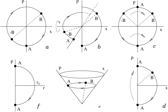
Figure 1: a. The phase-space plane $(p,x)$ and the oscillator trajectory on it. The states $B=(p,x)$ and $-B=(-p,-x)$ are gauge equivalent and to be identified;
b. The phase-space plane is cut along the $p$-axis. The half-plane $x<0$ is rotated relative to the $x$-axis through the angle $\pi$.
c. The resulting plane is folded along the $p$-axis so that the states $B$ and $-B$ get identified;
d. Two copies of each state on the $p$-axis, which occur upon the cut (e.g., the state $A$), are glued back to remove this doubling;
e. The resulting conic phase space. Each point of it corresponds to one physical state of the gauge system. The oscillator trajectory does not have any discontinuity;
f. The physical motion of the harmonic oscillator in the local gauge invariant variables $(p_{r},r)$. The trajectory has a discontinuity at the state A. The discontinuity occurs through the cut of the cone along the momentum axis. The cut is associated with the $(p_{r},r)$ parameterization of the cone.

Variations of $y^{a}$ generate simultaneous SO(N)-rotations of the vectors ${\bf x}(t)$ and ${\bf p}(t)$ as follows from the representations (3.6) and (3.26). Therefore, with an appropriate choice of the arbitrary functions $y^{a}(t)$, the physical motion can be described in two-dimensional phase space

$$x^{i}(t)=x(t)\delta^{i1}\ ,\ \ p_{i}(t)=\lambda(t)x(t)\delta_{i1}\equiv p(t)\delta_{i1}\ .$$ (3.28)

An important observation is the following [9]. Whenever the variable $x(t)$ changes sign under the gauge transformation (3.17), so does the canonical momentum $p(t)$ because of the constraint (3.26) or (3.28). In other words, for any motion in the phase-space plane two states $(p,x)$ and $(-p,-x)$ are physically indistinguishable. Identifying these points on the plane, we obtain the physical phase space of the system which is a cone unfoldable into a half-plane [9, 10]

$${\rm PS}_{\rm phys}={\rm PS}|_{\sigma_{a}=0}/{\rm SO(N)}\sim{\rm I\kern-1.79993ptR}^{2}/Z\!\!\!Z_{2}\sim{\rm cone}(\pi)\ .$$ (3.29)

Figure 1 illustrates how the phase-space plane turns into the cone upon the identification of the points $(p,x)$ and $(-p,-x)$.

Now we can address the above issue about nonphysical singularities of the gauge invariant velocity $\dot{r}$. To simplify the discussion and to make it transparent, let us first take a harmonic oscillator as an example. To describe the physical motion, we choose gauge-invariant canonical coordinates $r(t)=|{\bf x}(t)|$ and $p_{r}(t)=({\bf x},{\bf p})/r$. The gauge invariance means that

$$\{r,\sigma_{a}\}=\{p_{r},\sigma_{a}\}=0\ ,$$ (3.30)

i.e., the evolution of the canonical pair $p_{r},r$ does not depend on arbitrary functions $y^{a}(t)$. Making use of (3.15) and (3.16) we find

$$r(t) = r_{0}|\cos\omega t|\ ;$$ (3.31)

$$p_{r}(t) = \lambda(t)r(t)=\dot{r}(t)=-\omega r_{0}\sin\omega t\,\,\varepsilon(\cos\omega t)\ .$$ (3.32)

Here the constant $\varphi_{0}$ has been set to zero, and $r_{0}=|{\bf{x}}_{0}|$. The trajectory starts at the phase-space point $(0,r_{0})$ and goes down into the area of negative momenta as shown in Fig. 1f. At the time $t_{A}=\pi/2\omega$, the trajectory reaches the half-axis $p_{r}<0,r=0$ (the state $A$ in Fig. 1f). The physical momentum $p_{r}(t)$ has the sign flip as if the particle hits a wall. At that instant the acceleration is infinite because $\Delta p_{r}(t_{A})=p_{r}(t_{A}+\epsilon)-p_{r}(t_{A}-\epsilon)\rightarrow 2r_{0}\omega\ ,\epsilon\rightarrow 0$, which is not possible as the oscillator potential vanishes at the origin. Now we recall that the physical phase space of the model is a cone unfoldable into a half-plane. To parameterize the cone by the local gauge-invariant phase-space coordinates (3.32), (3.31), one has to make a cut of the cone along the momentum axis, which is readily seen from the comparison of figures 1d and 1f where the same motion is represented. The states $(r_{0}\omega,0)$ and $(-r_{0}\omega,0)$ are two images of one state that lies on the cut made on the cone. Thus, in the conic phase space, the trajectory is smooth and does not contains any discontinuities. The nonphysical “wall” force is absent (see Fig.1e).

In our discussion, a particular form of the potential $V$ has been assumed. This restriction can easily be dropped. Consider a trajectory $x^{i}(t)=x(t)\delta^{i1}$ passing through the origin at $t=t_{0},\ x(t_{0})=0$. In the physical variables the trajectory is $r(t)=|x(t)|$ and $p_{r}(t)=\dot{r}(t)=p(t)\varepsilon(x(t))$ where $p(t)=\dot{x}(t)$. Since the points $(p,x)$ and $(-p,-x)$ correspond to the same physical state, we find that the phase-space points $(p_{r}(t_{0}-\epsilon),x(t_{0}-\epsilon))$ and $(p_{r}(t_{0}+\epsilon),x(t_{0}+\epsilon))$ approach the same physical state as $\epsilon$ goes to zero. So, for any trajectory and any regular potential the discontinuity $|p_{r}(t_{0}-\epsilon)-p_{r}(t_{0}+\epsilon)|\rightarrow 2|p(t_{0})|$, as $\epsilon\rightarrow 0$, is removed by going over to the conic phase space.

The observed singularities of the phase-space trajectories are essentially artifacts of the coordinate description and, hence, depend on the parameterization of the physical phase space. For instance, the cone can be parameterized by another set of canonical gauge-invariant variables

$$p_{r}=|{\bf p}|\geq 0\ ,\ \ r=\frac{({\bf p},{\bf x})}{p_{r}}\ ,\ \ \{r,p_{r}\}=1\ .$$ (3.33)

It is easy to convince oneself that $r(t)$ would have discontinuities, rather than the momentum $p_{r}$. This set of local coordinates on the physical phase space is associated with the cut on the cone along the coordinate axis. In general, local canonical coordinates on the physical phase space are determined up to canonical transformations

$$(p_{r},r)\rightarrow(P_{R},R)=(P_{R}(r,p_{r}),R(p_{r},r))\ ,\ \ \ \ \{R,P_{R}\}=1\ .$$ (3.34)

The coordinate singularities associated with arbitrary local canonical coordinates on the physical phase space may be tricky to analyze. However, the motion considered on the true physical phase space is free of these ambiguities. That is why it is important to establish the geometry of the physical phase space before studying Hamiltonian dynamics in some local formally gauge invariant canonical coordinates.

It is also of interest to find out whether there exist a set of canonical variables in which the discontinuities of the classical phase-space trajectories do not occur. Let us return to the local coordinates where the momentum $p_{r}$ changes sign as the trajectory passes through the origin $r=0$. The sought-for new canonical variables must be even functions of $p_{r}$ when $r=0$ and be regular on the half-plane $r\geq 0$. Then the trajectory in the new coordinates will not suffer the discontinuity. In the vicinity of the origin, we set

$$R=a_{0}(p_{r}^{2})+\sum_{n=1}^{\infty}a_{n}(p_{r})r^{n}\ ,\ \ \ \ P_{R}=b_{0}(p_{r}^{2})+\sum_{n=1}^{\infty}b_{n}(p_{r})r^{n}\ .$$ (3.35)

Comparing the coefficients of powers of $r$ in the Poisson bracket (3.34) we find, in particular,

$$2p_{r}\left[a_{1}(p_{r})b_{0}^{\prime}(p_{r}^{2})-a_{0}^{\prime}(p_{r}^{2})b_{1}(p_{r})\right]=1\ .$$ (3.36)

Equation (3.36) has no solution for regular functions $a_{0,1}$ and $b_{0,1}$. By assumption the functions $a_{n}$ and $b_{n}$ are regular and so should be $a_{1}b_{0}^{\prime}-a_{0}^{\prime}b_{1}=1/(2p_{r})$, but the latter is not true at $p_{r}=0$ as follows from (3.36). A solution exists only for functions singular at $p_{r}=0$. For instance, one can take $R=r/p_{r}$ and $P_{R}=p_{r}^{2}/2$, $\{R,P_{R}\}=1$ which is obviously singular at $p_{r}=0$. In these variables the evolution of the canonical momentum does not have abrupt jumps, however, the new canonical coordinate does have jumps as the system goes through the states with $p_{r}=0$.

In general, the existence of singularities are due to the condition that $a_{0}$ and $b_{0}$ must be even functions of $p_{r}$. This latter condition leads to the factor $2p_{r}$ in the left-hand side of Eq.(3.36), thus making it impossible for $b_{1}$ and $a_{1}$ to be regular everywhere. We conclude that, although in the conic phase space the trajectories are regular, the motion always exhibits singularities when described in any local canonical coordinates on the phase space.

Our analysis of the simple gauge model reveals an important and rather general feature of gauge theories. The physical phase space in gauge theories may have a non-Euclidean geometry. The phase-space trajectories are smooth in the physical phase space. However, when described in local canonical coordinates, the motion may exhibit nonphysical singularities. In Section 6 we show that the impossibility of constructing canonical (Darboux) coordinates on the physical phase space, which would provide a classical description without singularities, is essentially due to the nontrivial topology of the gauge orbits (the concentric spheres in this model). The singularities fully depend on the choice of local canonical coordinates, even though this choice is made in a gauge-invariant way. What remains coordinate- and gauge-independent is the geometrical structure of the physical phase space which, however, may reveal itself through the coordinate singularities occurring in any particular parameterization of the physical phase space by local canonical variables. One cannot assign any direct physical meaning to the singularities, but their presence indicates that the phase space of the physical degrees of freedom is not Euclidean. At this stage of our discussion it becomes evident that it is of great importance to find a quantum formalism for gauge theories which does not depend on local parameterization of the physical phase space and takes into account its genuine geometrical structure.

3.3 Symplectic structure on the physical phase space

The absence of local canonical coordinates in which the dynamical description does not have singularities may seem to look rather disturbing. This is partially because of our custom to often identify canonical variables with physical quantities which can be directly measured, like, for instance, positions and momenta of particles in classical mechanics. In gauge theories canonical variables, that are defined through the Legendre transformation of the Lagrangian, cannot always be measured and, in fact, may not even be physical quantities. For example, canonical variables in electrodynamics are components of the electrical field and vector potential. The vector potential is subject to the gradient gauge transformations. So it is a nonphysical quantity.

The simplest gauge invariant quantity that can be built of the vector potential is the magnetic field. It can be measured. Although the electric and magnetic fields are not canonically conjugated variables, we may calculate the Poisson bracket of them and determine the evolution of all gauge invariant quantities (being functions of the electric and magnetic fields) via the Hamiltonian equation motion with the new Poisson bracket. Extending this analogy further we may try to find a new set of physical variables in the SO(N) model that are not necessarily canonically conjugated but have a smooth time evolution. A simple choice is

$$Q={\bf x}^{2}\ ,\ \ \ P=({\bf p},{\bf x})\ .$$ (3.37)

The variables (3.37) are gauge invariant and in a one-to-one correspondence with the canonical variables $r,p_{r}$ parameterizing the physical (conic) phase space: $Q=r^{2},P=p_{r}r,r\geq 0$. Due to analyticity in the original phase space variables, they also have a smooth time evolution $Q(t),P(t)$. However, we find

$$\{Q,P\}=2Q\ ,$$ (3.38)

that is, the symplectic structure is no longer canonical. The new symplectic structure is also acceptable to formulate Hamiltonian dynamics of physical degrees of freedom. The Hamiltonian assumes the form

$$H=\frac{1}{2Q}\,P^{2}+V(Q)\ .$$ (3.39)

Therefore

$$\dot{Q}=\{Q,H\}=2P\ ,\ \ \ \dot{P}=\{P,H\}=\frac{P^{2}}{Q}-2QV^{\prime}(Q)\ .$$ (3.40)

The solutions $Q(t)$ and $P(t)$ are regular for a sufficiently regular $V$, and there is no need to “remember” where the cut on the cone has been made.

The Poisson bracket (3.38) can be regarded as a skew-symmetric product (commutator) of two basis elements of the Lie algebra of the dilatation group. This observation allows one to quantize the symplectic structure. The representation of the corresponding quantum commutation relations is realized by the so called affine coherent states. Moreover the coherent-state representation of the path integral can also be developed [14], which is not a canonical path integral when compared with the standard lattice treatment.

3.4 The phase space in curvilinear coordinates

Except the simplest case when the gauge transformations are translations in the configuration space, physical variables are non-linear functions of the original variables of the system. The separation of local coordinates into the physical and pure gauge ones can be done by means of going over to curvilinear coordinates such that some of them span gauge orbits, while the others change along the directions transverse to the gauge orbits and, therefore, label physical states. In the example considered above, the gauge orbits are spheres centered at the origin. An appropriate coordinate system to separate physical and nonphysical variables is the spherical coordinate system. It is clear that dynamics of angular variables is fully arbitrary and determined by the choice of functions $y^{a}(t)$. In contrast the temporal evolution of the radial variable does not depend on $y^{a}(t)$. The phase space of the only physical degree of freedom turns out to be a cone unfoldable into a half-plane.

Let us forget about the gauge symmetry in the model for a moment. Upon a canonical transformation induced by going over to the spherical coordinates, the radial degree of freedom seems to have a phase space being a half-plane because $r=|{\bf x}|\geq 0$, and the corresponding canonical momentum would have an abrupt sign flip when the system passes through the origin. It is then natural to put forward the question whether the conic structure of the physical phase space is really due to the gauge symmetry, and may not emerge upon a certain canonical transformation. We shall argue that without the gauge symmetry, the full phase-space plane $(p_{r},r)$ is required to uniquely describe the motion of the system [10]. As a general remark, we point out that the phase-space structure cannot be changed by any canonical transformation. The curvature of the conic phase space, which is concentrated on the tip of the cone, cannot be introduced or even eliminated by any coordinate transformation.

For the sake of simplicity, the discussion is restricted to the simplest case of the $SO(2)$ group [10]. The phase space is a four-dimensional Euclidean space spanned by the canonical coordinates ${\bf p}\in{\rm I\kern-1.79993ptR}^{2}$ and ${\bf x}\in{\rm I\kern-1.79993ptR}^{2}$. For the polar coordinates $r$ and $\theta$ introduced by

$$x^{1}=r\cos\theta\ ,\ \ \ \ x^{2}=r\sin\theta\ ,$$ (3.41)

the canonical momenta are

$$p_{r}=\frac{({\bf x},{\bf p})}{r}\ ,\ \ \ \ p_{\theta}=({\bf p},T{\bf x})$$ (3.42)

with $T_{ij}=-T_{ji},\ T_{12}=1$, being the only generator of SO(2). The one-to-one correspondence between the Cartesian and polar coordinates is achieved if the latter are restricted to non-negative values for $r$ and to the segment $[0,2\pi)$ for $\theta$.

To show that the full plane $(p_{r},r)$ is necessary for a unique description of the motion, we compare the motion of a particle through the origin in Cartesian and polar coordinates, assuming the potential to be regular at the origin. Let the particle move along the $x^{1}$ axis. As long as the particle moves along the positive semiaxis the equality $x^{1}=r$ is satisfied and no paradoxes arise. As the particle moves through the origin, $x^{1}$ changes sign, $r$ does not change sign, and $\theta$ and $p_{r}$ change abruptly: $\theta\rightarrow\theta+\pi,\ p_{r}=|p|\cos\theta\rightarrow-p_{r}$. Although these jumps are not related with the action of any forces, they are consistent with the equations of motion. The kinematics of the system admits an interpretation in which the discontinuities are avoided. As follows from the transformation formulas (3.41), the Cartesian coordinates $x^{1,2}$ remains unchanged under the transformations

$$\theta \rightarrow \theta+\pi\ ,\ \ \ \ \ \ r\rightarrow-r\ ;$$ (3.43)

$$\theta \rightarrow \theta+2\pi\ ,\ \ \ \ \ r\rightarrow r\ .$$ (3.44)

This means that the motion with values of the polar coordinates $\theta+\pi$ and $r>0$ is indistinguishable from the motion with values of the polar coordinates $\theta$ and $r<0$. Consequently, the phase-space points $(p_{r},r;p_{\theta},\theta)$ and $(-p_{r},-r;\theta+\pi,p_{\theta})$ correspond to the same state of the system. Therefore, the state $(-p_{r},r;p_{\theta},\theta+\pi)$ the particle attains after passing through the origin is equivalent to $(p_{r},-r;p_{\theta},\theta)$. As expected, the phase-space trajectory will be identical in both the $(p_{r},r)-$plane and the $(p_{1},x^{1})-$plane.

Figure 2: a. A phase-space trajectory of a harmonic oscillator. The initial condition are such that $x^{2}=p_{2}=0$ for all moments of time. The system moves through the origin $x^{1}=0$;
b. The same motion is represented in the canonical variables associated with the polar coordinates. When passing the origin $r=0$, the trajectory suffers a discontinuity caused by the jump of the canonical momenta. The discontinuity can be removed in two ways:
c. One can convert the motion with values of the canonical coordinates $(-p_{r},r;$ $p_{\theta},\theta+\pi)$ into the equivalent motion $(p_{r},-r;p_{\theta},\theta)$, thus making a full phase-space plane out of two half-planes.
d. Another possibility is to glue directly the points connected by the dashed lines. The resulting surface is the Riemann surface with two conic leaves. It has no curvature at the origin because the phase-space radius vector $(p_{r},r)$ sweeps the total angle $2\pi$ around the two conic leaves before returning to the initial state.

In Fig.2 it is shown how the continuity of the phase-space trajectories can be maintained in the canonical variables $p_{r}$ and $r$. The original trajectory in the Cartesian variables is mapped into two copies of the half-plane $r\geq 0$. Each half-plane corresponds to the states of the system with values of $\theta$ differing by $\pi$ (Fig. 2b). Using the equivalence between the states $(-p_{r},r;p_{\theta},\theta+\pi)$ and $(p_{r},-r;p_{\theta},\theta)$, the half-plane corresponding to the value of the angular value $\theta+\pi$ can be viewed as the half-plane with negative values of $r$ so that the trajectory is continuous on the $(p_{r},r)$-plane and the angular variables does not change when the system passes through the origin (Fig. 2c).

Another possibility to keep the trajectories continuous under the canonical transformation, while maintaining the positivity of $r$, is to glue the edges of the half-planes connected by the dashed lines in Fig. 2b. The resulting surface resembles the Riemann surface with two conic leaves (Fig. 2d). The curvature at the origin of this surface is zero because for any periodic motion the trajectory goes around both conic leaves before it returns to the initial state, i.e., the phase-space radius-vector $(r,p_{r})$ sweeps the total angle $2\pi$. Thus, the motion is indistinguishable from the motion in the phase-space plane.

When the gauge symmetry is switched on, the angular variable $\theta$ becomes nonphysical, the constraint is determined by $p_{\theta}=0$. The states which differ only by values of $\theta$ must be identified. Therefore two conic leaves of the $(p_{r},r)$-Riemann surface become two images of the physical phase space. By identifying them, the Riemann surface turns into a cone unfoldable into a half-plane. In the representation given in Fig. 2c, the cone emerges upon the familiar identification of the points $(-p_{r},-r)$ with $(p_{r},r)$. This follows from the equivalence of the states $(-p_{r},-r;p_{\theta}=0,\theta)\sim(p_{r},r;p_{\theta}=0,\theta+\pi)\sim(p_{r},r;p_{\theta}=0,\theta)$, where the first one is due to the symmetry of the change of variables, while the second one is due to the gauge symmetry: States differing by values of $\theta$ are physically the same.

3.5 Quantum mechanics on a conic phase space

It is clear from the correspondence principle that quantum theory should, in general, depend on the geometry of the phase space. It is most naturally exposed in the phase-space path integral representation of quantum mechanics. Before we proceed with establishing the path integral formalism for gauge theories whose physical phase space differs from a Euclidean space, let us first use simpler tools, like Bohr-Sommerfeld semiclassical quantization, to get an idea of how the phase space geometry in gauge theory may affect quantum theory [9], [10].

Let the potential $V$ of the system be such that there exist periodic solutions of the classical equations of motion. According to the Bohr-Sommerfeld quantization rule, the energy levels can be determined by solving the equation

$$W(E)=\oint pdq=\int_{0}^{T}p\dot{q}dt=2\pi\hbar\left(n+\frac{1}{2}\right)\ ,\ \ n=0,1,\ldots\ ,$$ (3.45)

where the integral is taken over a periodic phase-space trajectory with the period $T$ which may depend on the energy $E$ of the system. The quantization rule (3.45) does not depend on the parameterization of the phase space because the functional $W(E)$ is invariant under canonical transformations:$\oint pdq=\oint PdQ$ and, therefore, coordinate-free. For this reason we adopt it to analyze quantum mechanics on the conic phase space. For a harmonic oscillator of frequency $\omega$ and having a Euclidean phase space, the Bohr-Sommerfeld rule gives exact energy levels. Indeed, classical trajectories are

$$q(t)=\frac{\sqrt{2E}}{\omega}\sin\omega t\ ,\ \ p(t)=\sqrt{2E}\cos\omega t\ ,$$ (3.46)

thus leading to

$$E_{n}=\hbar\omega\left(n+\frac{1}{2}\right)\ ,\ \ n=0,1,\ldots\ .$$ (3.47)

In general, the Bohr-Sommerfeld quantization determines the spectrum in the semiclassical approximation (up to higher orders of $\hbar$) [15]. So our consideration is not yet a full quantum theory. Nonetheless it will be sufficient to qualitatively distinguish between the influence of the non-Euclidean geometry of the physical phase space and the effects of potential forces on quantum gauge dynamics.

Will the spectrum (3.47) be modified if the phase space of the system is changed to a cone unfoldable into a half-plane? The answer is affirmative [9, 10, 16]. The cone is obtained by identifying points on the plane related by reflection with respect to the origin, ${\rm cone}(\pi)\sim{\rm I\kern-1.79993ptR}^{2}/Z\!\!\!Z_{2}$. Under the residual gauge transformations $(p,q)\rightarrow(-p,-q)$, the oscillator trajectory maps into itself. Thus on the conic phase space it remains a periodic trajectory. However the period is twice less than that of the oscillator with a flat phase space because the states the oscillator passes at $t\in[0,\pi/\omega)$ are physically indistinguishable from those at $t\in[\pi/\omega,2\pi/\omega)$. Therefore the oscillator with the conic phase space returns to the initial state in two times faster than the ordinary oscillator:

$$T_{c}=\frac{1}{2}T=\frac{\pi}{\omega}\ .$$ (3.48)

The Bohr-Sommerfeld quantization rule leads to the spectrum

$$E^{c}_{n}=2E_{n}=2\hbar\omega\left(n+\frac{1}{2}\right)\ ,\ \ n=0,1,\ldots\ .$$ (3.49)

The distance between energy levels is doubled as though the physical frequency of the oscillator were $\omega_{\rm phys}=2\omega$. Observe that the frequency as the parameter of the Hamiltonian is not changed. The entire effect is therefore due to the conic structure of the physical phase space.

Since the Bohr-Sommerfeld rule does not depend on the parameterization of the phase space, one can also apply it directly to the conic phase space. We introduce the polar coordinates on the phase space [9]

$$q=\sqrt{\frac{2P}{\omega}}\cos Q\ ,\ \ p=\sqrt{2\omega P}\sin Q\ .$$ (3.50)

Here $\{Q,P\}=1$. If the variable $Q$ ranges from $0$ to $2\pi$, then $(p,q)$ span the entire plane ${\rm I\kern-1.79993ptR}^{2}$. The local variables $(p,q)$ would span a cone unfoldable into a half-plane if one restricts $Q$ to the interval $[0,\pi)$ and identify the phase-space points $(p,q)$ of the rays $Q=0$ and $Q=\pi$. From (3.46) it follows that the new canonical momentum $P$ is proportional to the total energy of the oscillator

$$E=\omega P\ .$$ (3.51)

For the oscillator trajectory on the conic phase space, we have

$$W_{c}(E)=\oint\limits pdq=\oint\limits PdQ=\frac{E}{\omega}\int_{0}^{\pi}dQ=\frac{\pi E}{\omega}=2\pi\hbar\left(n+\frac{1}{2}\right)\ ,$$ (3.52)

which leads to the energy spectrum (3.49).

The curvature of the conic phase space is localized at the origin. One may expect that the conic singularity of the phase space does not affect motion localized in phase-space regions which do not contain the origin. Such motion would be indistinguishable from the motion in the flat phase space. The simplest example of this kind is the harmonic oscillator whose equilibrium is not located at the origin [9]. In the original gauge model, we take the potential

$$V=\frac{\omega^{2}}{2}\left(|{\bf x}|-r_{0}\right)^{2}\ .$$ (3.53)

The motion is easy to analyze in the local gauge invariant variables $(p_{r},r)$, when the cone is cut along the momentum axis.

Figure 3: a. Oscillator double-well potential;
b. Phase-space trajectories in the flat phase space. For $E<E_{0}$ there are two periodic trajectories associated with two minima of the double-well potential.
c. The same motion in the conic phase space. It is obtained from the corresponding motion in the flat phase space by identifying the points $(p,x)$ with $(-p,-x)$. The local coordinates $p_{r}$ and $r$ are related to the parameterization of the cone when the cut is made along the momentum axis (the states A and -A are the same).

As long as the energy does not exceed a critical value $E_{0}=\omega^{2}r^{2}_{0}/2$, i.e., the oscillator cannot reach the origin $r=0$, the period of classical trajectory remains $2\pi/\omega$. The Bohr-Sommerfeld quantization yields the spectrum of the ordinary harmonic oscillator (3.47). However the gauge system differs from the corresponding system with the phase space being a full plane. As shown in Fig. 3b, the latter system has two periodic trajectories with the energy $E<E_{0}$ associated with two minima of the oscillator double-well potential. Therefore in quantum theory the low energy levels must be doubly degenerate. Due to the tunneling effect the degeneracy is removed. Instead of one degenerate level with $E<E_{0}$ there must be two close levels (we assume $(E_{0}\,-\,E)/E_{0}$ $<\!\!<1$ to justify the word “close”). In contrast, there is no doubling of classical trajectories in the conic phase space (see Fig. 3c), and no splitting of the energy levels should be expected. These qualitative arguments can also be given a rigorous derivation in the framework of the instanton calculus. We shall return to this issue after establishing the path integral formalism for the conic phase space (see section 8.9).

When the energy is greater than $E_{0}$, the particle can go over the potential barrier. In the flat phase space there would be only one trajectory with fixed energy $E$ exceeding $E_{0}$. From the symmetry arguments it is also clear that this trajectory is mapped onto itself upon the reflection $(p,x)\rightarrow(-p,-x)$. Identifying these points of the flat phase space, we observe that the trajectory on the conic phase space with $E>E_{0}$ is continuous and periodic. In Fig. 3c the semiaxes $p_{r}<0$ and $p_{r}>0$ on the line $r=0$ are identified in accordance with the chosen parameterization of the cone.

Assume the initial state of the gauge system to be at the phase space point $O$ in Fig. 3c, i.e. $r(0)=r_{0}$. Let $t_{A}$ be the time when the system approaches the state $-A$. In the next moment of time the system leaves the state $A$. The states $A$ and $-A$ lie on the cut of the cone and, hence, correspond to the same state of the system. There is no jump of the physical momentum at $t=t_{A}$. From symmetry arguments it follows that the system returns to the initial state in the time

$$T_{c}=\frac{\pi}{\omega}+2t_{A}\ .$$ (3.54)

It takes $t=2t_{A}$ to go from the state $O$ to $-A$ and then from $A$ to $O^{\prime}$. From the state $O^{\prime}$ the system reaches the initial state $O$ in half of the period of the harmonic oscillator, $\pi/\omega$. The time $t_{A}$ depends on the energy of the system and is given by

$$t_{A}=\frac{1}{\omega}\sin^{-1}\sqrt{\frac{E_{0}}{E}}\leq\frac{\pi}{2\omega}\ ,\ \ \ \ \ E\geq E_{0}\ .$$ (3.55)

The quasiclassical quantization rule yields the equation for energy levels

$$W_{c}(E) = W(E)-2E\int_{t_{A}}^{\frac{\pi}{\omega}-t_{A}}\cos^{2}\omega t\,dt$$ (3.56)

$$= W(E)\left(\frac{1}{2}+\frac{\omega t_{A}}{\pi}+\frac{1}{2\pi}\,\sin 2\omega t_{A}\right)=2\pi\hbar\left(n+\frac{1}{2}\right)\ .$$

Here $W(E)=2\pi E/\omega$ is the Bohr-Sommerfeld functional for the harmonic oscillator of frequency $\omega$. The function $W_{c}(E)$ for the conic phase space is obtained by subtracting a contribution of the portion of the ordinary oscillator trajectory between the states $-A$ and $A$ for negative values of the canonical coordinate, i.e., for $t\in[t_{A},\pi/\omega-t_{A}]$. When the energy is sufficiently large, $E>\!\!>E_{0}$, the time $2t_{A}$ is much smaller than the half-period $\pi/\omega$, and $W_{c}(E)\sim\frac{1}{2}W(E)$, leading to the doubling of the distance between the energy levels. In this case typical fluctuations have the amplitude much larger than the distance from the classical vacuum to the singular point of the phase space. The system “feels” the curvature of the phase space localized at the origin. For small energies as compared with $E_{0}$, typical quantum fluctuations do not reach the singular point of the phase space. The dynamics is mostly governed by the potential force, i.e., the deviation of the phase space geometry from the Euclidean one does not affect much the low energy dynamics (cf. (3.56) for $t_{A}\approx\pi/(2\omega)$). As soon as the energy attains the critical value $E_{0}$ the distance between energy levels starts growing, tending to its asymptotic value $\Delta E=2\hbar\omega$.

The quantum system may penetrate into classically forbidden domains. The wave functions of the states with $E<E_{0}$ do not vanish under the potential barrier. So even for $E<E_{0}$ there are fluctuations that can reach the conic singularity of the phase space. As a result a small shift of the oscillator energy levels for $E<\!\!<E_{0}$ occurs. The shift can be calculated by means of the instanton technique. It is easy to see that there should exist an instanton solution that starts at the classical vacuum $r=r_{0}$, goes to the origin and then returns back to the initial state. We postpone the instanton calculation for later. Here we only draw the attention to the fact that, though in some regimes the classical dynamics may not be sensitive to the phase space structure, in the quantum theory the influence of the phase space geometry on dynamics may be well exposed.

The lesson we could learn from this simple qualitative consideration is that both the potential force and the phase space geometry affect the behavior of the gauge system. In some regimes the dynamics is strongly affected by the non-Euclidean geometry of the phase space. But there might also be regimes where the potential force mostly determines the evolution of the gauge system, and only a little of the phase-space structure influence can be seen. Even so, the quantum dynamics may be more sensitive to the non-Euclidean structure of the physical phase space than the classical one.

4 Systems with many physical degrees of freedom

So far only gauge systems with a single physical degree of freedom have been considered. A non-Euclidean geometry of the physical configuration or phase spaces may cause a specific kinematic coupling between physical degrees of freedom [17]. The coupling does not depend on details of dynamics governed by some local Hamiltonian. One could say that the non-Euclidean geometry of the physical configuration or phase space reveals itself through observable effects caused by this kinematic coupling. We now turn to studying this new feature of gauge theories.

4.1 Yang-Mills theory with adjoint scalar matter in (0+1) spacetime

Consider Yang-Mills potentials $A_{\mu}({\bf x},t)$. They are elements of a Lie algebra $X$ of a semisimple compact Lie group $G$. In the (0+1) spacetime, the vector potential has one component, $A_{0}$, which can depend only on time $t$. This only component is denoted by $y(t)$. Introducing a scalar field in (0+1) spacetime in the adjoint representation of $G$, $x=x(t)\in X$, we can construct a gauge invariant Lagrangian using a simple dimensional reduction of the Lagrangian for Yang-Mill fields coupled to a scalar field in the adjoint representation [18, 19]

$$L = \frac{1}{2}\left(D_{t}x,D_{t}x\right)-V(x)\ ,$$ (4.1)

$$D_{t}x = \dot{x}+i[y,x]\ .$$ (4.2)

Here $(\,,\,)$ stands for an invariant scalar product for the adjoint representation of the group. Let $\lambda_{a}$ be a matrix representation of an orthonormal basis in $X$ so that ${\rm tr}\,\lambda_{a}\lambda_{b}=\delta_{ab}$. Then we can make decompositions $y=y^{a}\lambda_{a}$ and $x=x^{a}\lambda_{a}$ with $y^{a}$ and $x^{a}$ being real. The invariant scalar product can be normalized on the trace $(x,y)={\rm tr}\,xy$. The commutator in (4.2) is specified by the commutation relation of the basis elements

$$[\lambda_{a},\lambda_{b}]=if_{ab}{}^{c}\lambda_{c}\ ,$$ (4.3)

where $f_{ab}{}^{c}$ are the structure constants of the Lie algebra.

The Lagrangian (4.1) is invariant under the gauge transformations

$$x\rightarrow x^{\Omega}=\Omega x\Omega^{-1}\ ,\ \ \ \ y\rightarrow y^{\Omega}=\Omega y\Omega^{-1}+i\dot{\Omega}\Omega^{-1}\ ,$$ (4.4)

where $\Omega=\Omega(t)$ is an element of the group $G$. Here the potential $V$ is also assumed to be invariant under the adjoint action of the group on its argument, $V(x^{\Omega})=V(x)$. The Lagrangian does not depend on the velocities $\dot{y}$. Therefore the corresponding Euler-Lagrange equations yield a constraint

$$-\frac{\partial L}{\partial y}=i[x,D_{t}x]=0\ .$$ (4.5)

This is the Gauss law for the model (cf. with the Gauss law in the electrodynamics or Yang-Mills theory). Note that it involves no second order time derivatives of the dynamical variable $x$ and, hence, only implies restrictions on admissible initial values of the velocities and positions with which the dynamical equation

$$D_{t}^{2}x=-V^{\prime}_{x}$$ (4.6)

is to be solved. The Yang-Mills degree of freedom $y$ appears to be purely nonphysical; its evolution is not determined by the equations of motion. It can be removed from them and the constraint (4.5) by the substitution

$$x(t)=U(t)h(t)U^{-1}(t)\ ,\ \ \ \ U(t)={\rm T}\exp\left\{-i\int_{0}^{t}d\tau y(\tau)\right\}\ .$$ (4.7)

In doing so, we get

$$[h,\dot{h}]=0\ ,\ \ \ \ \ddot{h}=-V_{h}^{\prime}\ .$$ (4.8)

The freedom in choosing the function $y(t)$ can be used to remove some components of $x(t)$ (say, to set them to zero for all moments of time). This would imply the removal of nonphysical degrees of freedom of the scalar field by means of gauge fixing, just as we did for the SO(N) model above. Let us take $G=SU(2)$. The orthonormal basis reads $\lambda_{a}=\tau_{a}/\sqrt{2}$, where $\tau_{a},a=1,2,3,$ are the Pauli matrices, $\tau_{a}\tau_{b}=\delta_{ab}+i\varepsilon_{abc}\tau_{c}$; $\varepsilon_{abc}$ is the totally antisymmetric structure constant tensor of SU(2), $\varepsilon_{123}=1$. The variable $x$ is a hermitian traceless $2\times 2$ matrix which can be diagonalized by means of the adjoint transformation (4.7). Therefore one may always set $h=h^{3}\lambda_{3}$. All the continuous gauge arbitrariness is exhausted, and the real variable $h^{3}$ describes the only physical degree of freedom. However, whenever this variable attains, say, negative values as time proceeds, the gauge transformation $h\rightarrow-h$ can still be made. For example, taking $U=e^{i\pi\tau_{2}/2}$ one find $U\tau_{3}U^{-1}=\tau_{2}\tau_{3}\tau_{2}=-\tau_{3}$. Thus, the physical values of $h^{3}$ lie on the positive half-axis. We conclude that

$${\rm CS}_{\rm phys}=su(2)/{\rm ad}SU(2)\sim{\rm I\kern-1.79993ptR}_{+}\ ,\ \ \ \ \ {\rm CS}=X=su(2)\sim{\rm I\kern-1.79993ptR}^{3}\ .$$ (4.9)

It might look surprising that the system has physical degrees of freedom at all because the number of gauge variables $y^{a}$ exactly equals the number of degrees of freedom of the scalar field $x^{a}$. The point is that the variable $h$ has a stationary group formed by the group elements $e^{i\varphi},[\varphi,h]=0$ and, hence, so does a generic element of the Lie algebra $x$. The stationary group is a subgroup of the gauge group. So the elements $U$ in (4.7) are specified modulo right multiplication on elements from the stationary group of $h$, $U\rightarrow Ue^{i\varphi}$. In the SU(2) example, the stationary group of $\tau_{3}$ is isomorphic to U(1), therefore the group element $U(t)$ in (4.7) belongs to SU(2)/U(1) and has only two independent parameters, i.e., the scalar field $x$ carries one physical and two nonphysical degrees of freedom. From the point of view of the general constrained dynamics, the constraints (4.5) are not all independent. For instance, ${\rm tr}\,(\varphi[x,D_{t}x])=0$ for all $\varphi$ commuting with $x$. Such constraints are called reducible (see [20, 21] for a general discussion of constrained systems). Returning to the SU(2) example, one can see that among the three constraints only two are independent, which indicates that there are only two nonphysical degrees of freedom contained in $x$.

To generalize our consideration to an arbitrary group $G$, we would need some mathematical facts from group theory. The reader familiar with group theory may skip the following section.

4.2 The Cartan-Weyl basis in Lie algebras

Any simple Lie algebra $X$ is characterized by a set of linearly independent $r$-dimensional vectors $\vec{\omega}_{j},\ j=1,2,...,r={\rm rank}\ X$, called simple roots. The simple roots form a basis in the root system of the Lie algebra. Any root $\vec{\alpha}$ is a linear combination of $\vec{\omega}_{j}$ with either non-negative integer coefficients ($\vec{\alpha}$ is said to be a positive root) or non-positive integer coefficients ($\vec{\alpha}$ is said to be a negative root). Obviously, all simple roots are positive. If $\vec{\alpha}$ is a root then $-\vec{\alpha}$ is also a root. The root system is completely determined by the Cartan matrix $c_{ij}=-2(\vec{\omega}_{i},\vec{\omega}_{j})/(\vec{\omega}_{j},\vec{\omega}_{j})$ (here $(\vec{\omega}_{i},\vec{\omega}_{j})$ is a usual Euclidean scalar product of two $r$-vectors) which has a graphic representation known as the Dynkin diagrams [30, 32]. Elements of the Cartan matrix are integers. For any two roots $\vec{\alpha}$ and $\vec{\beta}$, the cosine of the angle between them can take only the following values $(\vec{\alpha},\vec{\beta})[(\vec{\alpha},\vec{\alpha})(\vec{\beta},\vec{\beta})]^{-1/2}=0,\pm 1/2,\pm 1/\sqrt{2},\pm\sqrt{3}/2$. By means of this fact the whole root system can be restored from the Cartan matrix [30], p.460.

For any two elements $x,\ y$ of $X$, the Killing form is defined as $(x,y)={\rm tr}\,({\rm ad}\,{x}{\rm ad}\,{y})=(y,x)$ where the operator ${\rm ad}\,{x}$ acts on any element $y\in X$ as ${\rm ad}\,{x}(y)=[x,y]$ where $[x,y]$ is a skew-symmetric Lie algebra product that satisfies the Jacobi identity $[[x,y],z]+[[y,z],x]+[[z,x],y]=0$ for any three elements of the Lie algebra. A maximal Abelian subalgebra $H$ in $X$ is called the Cartan subalgebra, $\dim H={\rm rank}\ X=r$. There are $r$ linearly independent elements $\omega_{j}$ in $H$ such that $(\omega_{i},\omega_{j})=(\vec{\omega}_{i},\vec{\omega}_{j})$. We shall also call the algebra elements $\omega_{i}$ simple roots. It will not lead to any confusing in what follows because the root space ${\rm I\kern-1.79993ptR}^{r}$ and the Cartan subalgebra are isomorphic, but we shall keep arrows over elements of ${\rm I\kern-1.79993ptR}^{r}$. The corresponding elements of $H$ have no over-arrow.

A Lie algebra $X$ is decomposed into the direct sum $X=H\oplus\sum_{\alpha>0}(X_{\alpha}\oplus X_{-\alpha}),\ \alpha$ ranges over the positive roots, $\dim X_{\pm\alpha}=1$. Simple roots form a basis (non-orthogonal) in $H$. Basis elements $e_{\pm\alpha}$ of $X_{\pm\alpha}$ can be chosen such that [30], p.176,

$$\left[e_{\alpha},e_{-\alpha}\right] = \alpha\ ,$$ (4.10)

$$\left[h,e_{\alpha}\right] = (\alpha,h)e_{\alpha}\ ,$$ (4.11)

$$\left[e_{\alpha},e_{\beta}\right] = N_{\alpha,\beta}e_{\alpha+\beta}\ ,$$ (4.12)

for all $\alpha,\beta$ belonging to the root system and for any $h\in H$, where the constants $N_{\alpha,\beta}$ satisfy $N_{\alpha,\beta}=-N_{-\alpha,-\beta}$. For any such choice $N_{\alpha,\beta}^{2}=1/2q(1-p)(\alpha,\alpha)$ where $\beta+n\alpha\ (p\leq n\leq q)$ is the $\alpha$-series of roots containing $\beta$; $N_{\alpha,\beta}=0$ if $\alpha+\beta$ is not a root. Any element $x\in X$ can be decomposed over the Cartan-Weyl basis (4.10)–(4.12),

$$x=x_{H}+\sum_{\alpha>0}(x^{\alpha}e_{\alpha}+x^{-\alpha}e_{-\alpha})$$ (4.13)

with $x_{H}$ being the Cartan subalgebra component of $x$.

The commutation relations (4.10)–(4.12) imply a definite choice of the norms of the elements $e_{\pm\alpha}$, namely, $(e_{\pm\alpha},e_{\pm\alpha})=0$ and $(e_{\alpha},e_{-\alpha})=1$ [30], p.167. Norms of simple roots are also fixed in (4.10)–(4.12). Consider, for instance, the su(2) algebra. There is just one positive root $\omega$. Let its norm be $\gamma=(\omega,\omega)$. The Cartan-Weyl basis reads $[e_{\omega},e_{-\omega}]=\omega$ and $[\omega,e_{\pm\omega}]=\pm\gamma e_{\pm\omega}$. Let us calculate $\gamma$ in this basis. By definition $\gamma={\rm tr}\,({\rm ad}\,{\omega})^{2}$. The operator ${\rm ad}\,{\omega}$ is a $3\times 3$ diagonal matrix with $0,\pm\gamma$ being its diagonal elements as follows from the basis commutation relations and the definition of the operator ${\rm ad}\,{\omega}$. Thus, ${\rm tr}\,({\rm ad}\,{\omega})^{2}=2\gamma^{2}=\gamma$, i.e. $\gamma=1/2$.

The su(3) algebra has two equal-norm simple roots $\vec{\omega}_{1}$ and $\vec{\omega}_{2}$ with the angle between them equal to $2\pi/3$. For the corresponding Cartan subalgebra elements we have $(\omega_{1},\omega_{1})=(\omega_{2},\omega_{2})=\gamma$ and $(\omega_{1},\omega_{2})=-\gamma/2$. The whole root system is given by six elements $\pm\omega_{1},\pm\omega_{2}$ and $\pm(\omega_{1}+\omega_{2})\equiv\pm\omega_{12}$. It is readily seen that $(\omega_{12},\omega_{12})=\gamma$ and $(\omega_{1},\omega_{12})=(\omega_{2},\omega_{12})=\gamma/2$. All the roots have the same norm and the angle between two neighbor roots is equal to $\pi/3$. Having obtained the root pattern, we can evaluate the number $\gamma$. The (non-orthogonal) basis consists of eight elements $\omega_{1,2},\ e_{\pm 1},\ e_{\pm 2}$ and $e_{\pm 12}$ where we have introduced simplified notations $e_{\pm\omega_{1}}\equiv e_{\pm 1}$, etc. The operators ${\rm ad}{\omega}_{1,2}$ are $8\times 8$ diagonal matrices as follows from (4.11) and $[\omega_{1},\omega_{2}]=0$. Using (4.11) we find ${\rm tr}\,({\rm ad}\,{\omega}_{1,2})^{2}=3\gamma^{2}=\gamma$ and, therefore, $\gamma=1/3$. As soon as root norms are established, one can obtain the structure constants $N_{\alpha,\beta}$. For $X=su(3)$ we have $N_{1,2}^{2}=N_{12,-1}^{2}=N_{12,-2}^{2}=1/6$ and all others vanish (notice that $N_{\alpha,\beta}=-N_{-\alpha,-\beta}$ and $N_{\alpha,\beta}=-N_{\beta,\alpha}$). The latter determines the structure constants up to a sign. The transformation $e_{\alpha}\rightarrow-e_{\alpha},\ N_{\alpha,\beta}\rightarrow-N_{\alpha,\beta}$ leaves the Cartan-Weyl commutation relations unchanged. Therefore, only relative signs of the structure constants must be fixed. Fulfilling the Jacobi identity for elements $e_{-1},\ e_{1},\ e_{2}$ and $e_{-2},\ e_{1},\ e_{2}$ results in $N_{1,2}=-N_{12,-1}$ and $N_{1,2}=N_{12,-2}$, respectively. Now one can set $N_{1,2}=N_{12,-2}=-N_{12,-1}=1/\sqrt{6}$, which completes determining the structure constants for $su(3)$.

One can construct a basis orthonormal with respect to the Killing form. With this purpose we introduce the elements [30], p.181,

$$s_{\alpha}=i(e_{\alpha}-e_{-\alpha})/\sqrt{2},\ \ \ \ \ \ c_{\alpha}=(e_{\alpha}+e_{-\alpha})/\sqrt{2}\$$ (4.14)

so that

$$[h,s_{\alpha}]=i(h,\alpha)c_{\alpha}\ ,\ \ \ [h,c_{\alpha}]=-i(h,\alpha)s_{\alpha}\ ,\ \ \ h\in H\ .$$ (4.15)

Then $(s_{\alpha},s_{\beta})=(c_{\alpha},c_{\beta})=\delta_{\alpha\beta}$ and $(c_{\alpha},s_{\beta})=0$. Also,

$$(x,x)=\sum_{\alpha>0}\left[(x^{\alpha}_{s})^{2}+(x_{c}^{\alpha})^{2}\right]+(x_{H},x_{H})\ ,$$ (4.16)

where $x_{s,c}^{\alpha}$ are real decomposition coefficients of $x$ in the orthonormal basis (4.14). Supplementing (4.14) by an orthonormal basis $\lambda_{j},\ (\lambda_{j},\lambda_{i})=\delta_{ij}$, of the Cartan subalgebra (it might be obtained by orthogonalizing the simple root basis of $H$), we get an orthonormal basis in $X$; we shall denote it $\lambda_{a}$, that is, for $a=j$, $\lambda_{a}$ ranges over the orthonormal basis in the Cartan subalgebra, and for $a=\alpha$ over the set $s_{\alpha},c_{\alpha}$.

Suppose we have a matrix representation of $X$. Then $(x,y)=c_{r}\,{\rm tr}\,\ (xy)$ where $xy$ means a matrix multiplication. The number $c_{r}$ depends on $X$. For classical Lie algebras, the numbers $c_{r}$ are listed in [30], pp.187-190. For example, $c_{r}=2(r+1)$ for $X=su(r+1)$. Using this, one can establish a relation of the orthonormal basis constructed above for su(2) and su(3) with the Pauli matrices and the Gell-Mann matrices [33], p.17, respectively. For the Pauli matrices we have $[\tau_{a},\tau_{b}]=2i\varepsilon_{abc}\tau_{c}$, hence, $(\tau_{a},\tau_{b})=-4\varepsilon_{ab^{\prime}c^{\prime}}\varepsilon_{bc^{\prime}b^{\prime}}=8\delta_{ab}=4{\rm tr}\,\ \tau_{a}\tau_{b}$ in full accordance with $c_{r}=2(r+1),\ r=1$. One can set $\omega=\tau_{3}/4,\ s_{\omega}=\varphi\tau_{1}$ and $c_{\omega}=\varphi\tau_{2}$ where $1/\varphi=2\sqrt{2}$. A similar analysis of the structure constants for the Gell-Mann matrices $\lambda_{a}$ [33], p.18, yields $\omega_{1}=\lambda_{3}/6,\ s_{1}=\varphi\lambda_{1},\ c_{1}=\varphi\lambda_{2},\ \omega_{2}=(\sqrt{3}\lambda_{8}-\lambda_{3})/12,\ s_{2}=\varphi\lambda_{6},\ c_{2}=\varphi\lambda_{7}\ ,\omega_{12}=(\sqrt{3}\lambda_{8}+\lambda_{3})/12,\ s_{12}=\varphi\lambda_{5}$ and $c_{12}=-\varphi\lambda_{4}$ where $1/\varphi=2\sqrt{3}$. This choice is not unique. Actually, the identification of non-diagonal generators $\lambda_{a},\ a\neq 3,8$ with (4.14) depends on a representation of the simple roots $\omega_{1,2}$ by the diagonal matrices $\lambda_{3,8}$. One could choose $\omega_{1}=\lambda_{3}/6$ and $\omega_{2}=-(\sqrt{3}\lambda_{8}+\lambda_{3})/12$, which would lead to another matrix realization of the elements (4.14).

Consider the adjoint action of the group $G$ on its Lie algebra $X$: $x\rightarrow{\rm ad}\,U(x)$. Taking $U=e^{z},\,z\in X$, the adjoint action can be written in the form ${\rm ad}\,U=\exp(i{\rm ad}\,z)$. In a matrix representation it has a more familiar form, $x\rightarrow UxU^{-1}$. The Killing form is invariant under the adjoint action of the group

$$\left({\rm ad}\,U(x),{\rm ad}\,U(y)\right)=(x,y)\ .$$ (4.17)

In a matrix representation this is a simple statement: ${\rm tr}\,(UxU^{-1}UyU^{-1})={\rm tr}\,(xy)$. The Cartan-Weyl basis allows us to make computations without referring to any particular representation of a Lie algebra. This great advantage will often be exploited in what follows.

4.3 Elimination of nonphysical degrees of freedom. An arbitrary gauge group case.

The key fact for the subsequent analysis will be the following formula for a representation of a generic element of a Lie algebra [32]

$$x={\rm ad}\,U(h)\ ,\ \ \ U=U(z)=e^{iz}\ ,\ \ \ ({\rm or}\ \ x=UhU^{-1})\ ,$$ (4.18)

in which $h=h^{i}\lambda_{i}$ is an element of the Cartan subalgebra $H$ with an orthonormal basis $\lambda_{i},\,i=1,2,...,r={\rm rank}\,G$ and the group element $U(z)$ is obtained by the exponential map of $z=z^{\alpha}\lambda_{\alpha}\in X\ominus H$ to the group $G$. Here $\alpha=r+1,r+2,...,N={\rm dim}\,G$ and $z^{\alpha}$ are real. The $r$ variables $h^{i}$ are analogous to $h^{3}$ from the SU(2) example, while the variables $z^{\alpha}$ are nonphysical and can be removed by a suitable choice of the gauge variables $y^{a}$ for any actual motion as follows from a comparison of (4.18) and (4.7). Thus the rank of the Lie algebra specifies the number of physical degrees of freedom. The function $h(t)\in H$ describes the time evolution of the physical degrees of freedom. Note that the constraint in (4.8) is fulfilled identically, $[h,\dot{h}]\equiv 0$, because both the velocity and position are elements of the maximal Abelian (Cartan) subalgebra. We can also conclude that the original constraint (4.5) contains only $N-r$ independent equations.

There is still a gauge arbitrariness left. Just like in the SU(2) model, we cannot reduce the number of physical degrees of freedom, but a further reduction of the configuration space of the variable $h$ is possible. It is known [32] that a Lie group contains a discrete finite subgroup $W$, called the Weyl group, whose elements are compositions of reflections in hyperplanes orthogonal to simple roots of the Cartan subalgebra. The group $W$ is isomorphic to the group of permutations of the roots, i.e., to a group that preserves the root system. The gauge $x=h$ is called an incomplete global gauge with the residual symmetry group $W\subset G$ . The residual gauge symmetry can be used for a further reduction of the configuration space. The residual gauge group of the SU(2) model is $Z\!\!\!Z_{2}$ (the Weyl group for SU(2)) which identifies the mirror points $h^{3}$ and $-h^{3}$ on the real axis. One can also say that this group “restores” the real axis (isomorphic to the Cartan subalgebra of SU(2)) from the modular domain $h^{3}>0$. Similarly, the Weyl group $W$ restores the Cartan subalgebra from the modular domain called the Weyl chamber, $K^{+}\subset H$ [32] (up to the boundaries of the Weyl chamber being a zero-measure set in $H$).

The generators of the Weyl group are easy to construct in the Cartan-Weyl basis. The reflection of a simple root $\omega$ is given by the adjoint transformation: $\hat{R}_{\omega}\omega\equiv e^{i\varphi s_{\omega}}\omega e^{-i\varphi s_{\omega}}=-\omega$ where $\varphi=\pi/\sqrt{(\omega,\omega)}$. Any element of $W$ is obtained by a composition of $\hat{R}_{\omega}$ with $\omega$ ranging over the set of simple roots. The action of the generating elements of the Weyl group on an arbitrary element of the Cartan subalgebra reads

$$\hat{R}_{\omega}h=\Omega_{\omega}h\Omega_{\omega}^{-1}=h-\frac{2(h,\omega)}{(\omega,\omega)}\,\omega\ ,\ \ \ \ \Omega_{\omega}\in G\ .$$ (4.19)

The geometrical meaning of (4.19) is transparent. It describes a reflection of the vector $h$ in the hyperplane orthogonal to the simple root $\omega$. In what follows we assume the Weyl chamber to be an intersection of all positive half-spaces bounded by hyperplanes orthogonal to simple roots (the positivity is determined relative to the root vector direction). The Weyl chamber is said to be an open convex cone [35]. For any element $h\in K^{+}$, we have $(h,\omega)>0$ where $\omega$ ranges over all simple roots. Thus we conclude that

$${\rm CS}_{\rm phys}=X/{\rm ad}\,G\sim H/W\sim K^{+}\ .$$ (4.20)

The metric on the physical configuration space can be constructed as the induced metric on the surface $U(z)=e$ where $e$ is the group unity. First, the Euclidean metric $ds^{2}=(dx,dx)\equiv dx^{2}$ is written in the new curvilinear variables (4.18). Then one takes its inverse. The induced physical metric is identified with the inverse of the $hh$-block of the inverse of the total metric tensor. In doing so, we find

$$dx = {\rm ad}\,U(dh+[h,U^{-1}dU])\ ,$$

$$ds^{2} = dh^{2}+[h,U^{-1}dU]^{2}=\delta_{ij}dh^{i}dh^{j}+\tilde{g}_{\alpha\beta}(h,z)dz^{\alpha}dz^{\beta}\ ,$$ (4.21)

where we have used (4.17) and the fact that $[h,U^{-1}dU]\in X\ominus H$ (cf. (4.11)) and hence $(dh,[h,U^{-1}dU])=0$. The metric has a block-diagonal structure and so has its inverse. Therefore, the physical metric (the induced metric on the surface $z=0$) is the Euclidean one. The physical configuration space is a Euclidean space with boundaries (cf. (4.20)). It has the structure of an orbifold [36].

The above procedure of determining the physical metric is general for first-class constrained systems whose constraints are linear in momenta. The latter condition insures that the gauge transformations do not mix up the configuration and momentum space variables in the total phase space. There is an equivalent method of calculating the metric on the orbit space [13] which uses only a gauge condition. One takes the (Euclidean) metric on the original configuration space and obtains the physical metric by projecting tangent vectors (velocities) onto the subspace defined by the constraints. Since in what follows this procedure will also be used, we give here a brief description. Suppose we have independent first-class constraints $\sigma_{a}=F_{a}^{i}(q)p_{i}$. Consider the kinetic energy $H_{0}=g^{ij}p_{i}p_{j}/2\equiv g_{ij}v^{i}v^{j}/2$, where $g_{ij}$ is the metric on the total configuration space, $v^{i}=g^{ij}p_{j}$ tangent vectors, and $g^{ij}$ the inverse of the metric. We split the set of the canonical coordinates $q^{i}$ into two subsets $h^{\nu}$ and $\bar{q}{}^{a}$ such that the matrix $\{\bar{q}{}^{a},\sigma_{b}\}=F_{b}^{a}(q)$ is not degenerate on the surface $\bar{q}^{a}=0$ except, maybe, on a set of zero measure. Then the physical phase space can be parameterized by canonical coordinates $p_{\nu}$ and $h^{\nu}$. Denoting $\bar{F}_{a}^{b}(h)=F_{a}^{b}|_{\bar{q}=0}$, similarly $\bar{F}_{a}^{\nu}$ and $\bar{g}{}^{ij}$, we solve the constraints for nonphysical momenta $\bar{p}_{a}=-(\bar{F}^{-1})_{a}^{b}\bar{F}_{b}^{\nu}p_{\nu}\equiv\gamma_{b}^{\nu}p_{\nu}$ and substitute the result into the kinetic energy:

$$H_{0} = \frac{1}{2}g_{ph}^{\mu\nu}p_{\nu}p_{\mu}=\frac{1}{2}g^{ph}_{\mu\nu}v^{\mu}v^{\nu}\ ,$$ (4.22)

$$g_{ph}^{\mu\nu} = \bar{g}{}^{\mu\nu}-\gamma_{a}^{\mu}\bar{g}{}^{a\nu}-\bar{g}{}^{\mu a}\gamma_{a}^{\nu}+\gamma_{a}^{\mu}\bar{g}{}^{ab}\gamma_{b}^{\nu}\ ,$$ (4.23)

where $g^{ph}_{\mu\nu}$ is the inverse of $g^{\mu\nu}_{ph}$; it is the metric on the orbit space which determines the norm of the corresponding tangent vectors $v^{\mu}$ (physical velocities). Instead of conditions $\bar{q}=0$, one can use general conditions $\chi^{a}(q)=0$, which means that locally $\bar{q}=\bar{q}(h)$, where $h$ is a set of parameters to span the surface $\chi^{a}(q)=0$, instead of $\bar{q}=0$ in the above formulas. In the model under consideration, we set $x=h+z$, $h\in H$, and impose the condition $z=0$. Then setting $z$ equal zero in the constraint we obtain $[h,p_{z}]=0$ ($p_{z}\equiv\bar{p}$), which leads to $p_{z}=0$ as one can see from the commutation relation (4.11). Therefore $g_{ph}=1$ because $g=\bar{g}=1$.

It is also of interest to calculate the induced volume element $\mu(h)d^{r}h$ in ${\rm CS}_{\rm phys}$. In the curvilinear coordinates (4.18), the variables $z$ parameterize a gauge orbit through a point $x=h$. For $h\in K^{+}$, the gauge orbit is a compact manifold of dimension $N-r,\ \dim X=N$, and isomorphic to $G/G_{H}$ where $G_{H}$ is the maximal Abelian subgroup of $G$, the Cartan subgroup. The variables $h$ span the space locally transverse to the gauge orbits. So, the induced volume element can be obtained from the decomposition

$$d^{N}x=\sqrt{\det g}\,d^{N-r}zd^{r}h=\mu(h)d^{r}h\tilde{\mu}(z)d^{N-r}z\ .$$ (4.24)

Here $g$ is the metric tensor in (4.21). Making use of the orthogonal basis constructed in the previous subsection, the algebra element $U^{-1}dU$ can be represented in the form $-i\lambda_{a}F^{a}_{\alpha}(z)dz^{\alpha}$ with $F^{a}_{\alpha}$ being some functions of $z$. Their explicit form will not be relevant to us. Since the commutator $[\lambda_{i},\lambda_{\alpha}]$ always belongs to $X\ominus H$ and the $\lambda_{i}$’s are commutative, we find $[h,U^{-1}dU]=\lambda_{\gamma}h^{i}f_{i\alpha}{}^{\gamma}F^{\alpha}_{\beta}dz^{\beta}$. Hence,

$$\tilde{g}_{\alpha\beta}=F_{\alpha}^{\gamma}(z)G_{\gamma\delta}(h)F_{\beta}^{\delta}(z)\ ,\ \ \ \ G_{\alpha\beta}=\omega_{\alpha\gamma}\omega_{\beta}{}^{\gamma}\ ,\ \ \ \ \omega_{\alpha\beta}=h^{i}f_{i\alpha\beta}\ ,$$ (4.25)

and the Cartesian metric $\delta_{ab}=(\lambda_{a},\lambda_{b})$ is used to lower and rise the indices of the structure constants. Substituting these relations into the volume element (4.24) we obtain $\mu(h)=\det\omega(h)=\det(i{\rm ad}\,h)$. The latter determinant is quite easy to calculate in the orthogonalized Cartan-Weyl basis. Indeed, from (4.11) it follows that $[h,\lambda_{\alpha}]=i\omega_{\alpha}{}^{\beta}(h)\lambda_{\beta}$ and $\lambda_{\alpha}$ is the set (4.14). Let us order the basis elements $\lambda_{a}$ so that the first $r$ elements form the basis in the Cartan subalgebra, while $\lambda_{a}=s_{\alpha}$ and $\lambda_{a+1}=c_{\alpha}$ for $a=r+1,r+3,...,N-1$. An explicit form of the matrix $i\omega_{\alpha}{}^{\beta}$ is obtained from the commutation relations (4.15). It is block-diagonal, and each block is associated with the corresponding positive root $\alpha$ and equals $i(h,\alpha)\tau_{2}$ ($\tau_{2}$ being the Pauli matrix). Thus,

$$\mu(h)=\det(i{\rm ad}\,h)={\kappa}^{2}(h)\ ,\ \ \ \kappa(h)=\prod_{\alpha>0}(\alpha,h)\ .$$ (4.26)

The density $\mu$ is invariant under permutations and reflections of the roots, i.e., with respect to the Weyl group: $\mu(\hat{R}_{\omega}h)=\mu(h)$ for any simple root $\omega$. It also vanishes at the boundary of the Weyl chamber, $(\omega,h)=0$.

One should draw attention to the fact that the determinant of the induced metric on the physical configuration space does not yield the density. This is a generic situation in gauge theories [13]: In addition to the square root of the determinant of the physical metric, the density also contains a factor being the volume of the gauge orbit associated with each point of the gauge orbit space. In the model under consideration the physical configuration space has a Euclidean metric, and $\mu(h)$ determines the volume of the gauge orbit through the point $x=h$ up to a factor ($\int_{G/G_{H}}dz\tilde{\mu}(z)$) which is independent of $h$. For example, the adjoint action of SU(2) in its Lie algebra can be viewed as rotations in three dimensional Euclidean space. The gauge orbits are concentric two-spheres. In the spherical coordinates we have $d^{3}x=\sin\theta d\theta d\phi r^{2}dr$. The volume of a gauge orbit through $x^{i}=\delta^{i1}r$ is $4\pi r^{2}$. In (4.24) $z^{\alpha}$ are the angular variables $\theta$ and $\phi$, while $h$ is $r$, and $\tilde{\mu}=\sin\theta$, $\mu=r^{2}$.

4.4 Hamiltonian formalism

Now we develop the Hamiltonian formalism for the model and describe the structure of the physical phase space. The system has $N$ primary constraints $\pi_{a}=\partial L/\partial\dot{y}^{a}=0$. Its canonical Hamiltonian reads

$$H=\frac{1}{2}p^{2}+V(x)+y^{a}\sigma_{a}\ ,$$ (4.27)

where $p^{2}=(p,p)$, $p=\partial L/\partial\dot{x}=D_{t}x$ is the momentum conjugate to $x$ and

$$\sigma_{a}=i(\lambda_{a},[x,p])=0\ ,\ \ \ \{\sigma_{a},\sigma_{b}\}=if_{ab}{}^{c}\sigma_{c}$$ (4.28)

are the secondary constraints. They generate the gauge transformations on phase space given by the adjoint action of the group $G$ on its Lie algebra

$$p\rightarrow p^{\Omega}=\Omega p\Omega^{-1}\ ,\ \ \ \ x\rightarrow x^{\Omega}=\Omega x\Omega^{-1}\ ,$$ (4.29)

because $\{p,\sigma_{a}\}=i[\lambda_{a},p]$ and $\{x,\sigma_{a}\}=i[\lambda_{a},x]$. The Hamiltonian equations of motion do not specify the time evolution of the gauge variable $y$. So the phase space trajectory described by the pair $p(t),\,x(t)$ depends on the choice of $y(t)$. Trajectories associated with different functions $y(t)$ are related to one another by gauge transformations. Just like in the Lagrangian formalism, this gauge arbitrariness can be used to suppress dynamics of some degrees of freedom of the scalar field $x(t)$.

We choose the $y(t)$ so that $x(t)=h(t)\in H$. The constraint (4.28) means that the momentum and position should commute as Lie algebra elements, $[p,x]=0$. Therefore on the constraint surface, the canonical momentum $p_{h}$ conjugate to $h$ must commute with $h$, $[p_{h},h]=0$. This is a simple consequence of the gauge transformation law (4.29): If the variable $x(t)$ is brought to the Cartan subalgebra by a gauge transformation, then the same gauge transformation simultaneously applies to $p(t)$ turning it into $p_{h}(t)$. Since the constraint is covariant under gauge transformations, the new canonical variables $h$ and $p_{h}$ should also fulfill the constraint. Thus, we are led to the conclusion that $p_{h}$ is an element of the Cartan subalgebra because it commutes with a generic element $h\in H$. There is no more continuous gauge arbitrariness left, but a further reduction of the phase space is still possible. The variable $h$ has gauge equivalent configurations related to one another by the Weyl transformations. In the phase space spanned by the Cartan algebra elements $p_{h}$ and $h$, the Weyl group acts simultaneously on the momentum and position variables in accordance with the gauge transformation law (4.29). Thus,

$${\rm PS}_{\rm phys}\sim H\oplus H/W\sim{\rm I\kern-1.79993ptR}^{2r}/W\ .$$ (4.30)

By identifying the points $(\hat{R}p_{h},\hat{R}h),\,\hat{R}\in W$, the Euclidean space ${\rm I\kern-1.79993ptR}^{2r}$ turns into a $2r$-dimensional hypercone which, after an appropriate cut, is unfoldable into ${\rm I\kern-1.79993ptR}^{r}\oplus K^{+}$.

For generic configurations $h\in K^{+}$ the physical phase space has no singularities and is locally flat. When $h$ approaches a generic point on the boundary $(h,\omega)=0$ of the Weyl chamber, the physical phase space exhibits a conic singularity. Indeed, we may always make a linear canonical transformation such that one of the canonical coordinates, say $h^{\perp}$, varies along the line perpendicular to the boundary, while the others span hyperplanes parallel to the hyperplane $(h,\omega)=0$ being a part of the Weyl chamber boundary. In the new variables, the Weyl transformation that flips sign of the root $\omega$ will change signs of $h^{\perp}$ and its canonical momentum, while leaving the other canonical variables unchanged. Thus, at a generic point of the Weyl chamber boundary, the physical phase space has a local structure ${\rm I\kern-1.79993ptR}^{2(r-1)}\oplus cone(\pi)$.

The Weyl chamber boundary is not a smooth manifold and contains intersections of two hyperplanes $(\omega_{1},h)=0$ and $(\omega_{2},h)=0$. At these points, the two local conic singularities of the physical phase space associated with simple roots $\omega_{1,2}$ would merge, forming locally a 4-dimensional hyperconic singularity. This singularity cannot be simply described as a direct product of two cones $cone(\pi)$. It would only be the case if the roots $\omega_{1,2}$ are orthogonal. In general, the tip of the hypercone would be “sharper” than that of $cone(\pi)\oplus cone(\pi)$, meaning that the hypercone can always be put inside of $cone(\pi)\oplus cone(\pi)$ when their tips are at the same point. This can be understood again in the local canonical variables where the coordinates $h$ are split into a pair $h^{\perp}$ that spans a plane perpendicular to the intersection of two hyperplanes $(\omega_{1,2},h)=0$ and the others orthogonal to $h^{\perp}$. The root pattern in any plane containing at least two roots (e.g., a plane through the origin and parallel to the $h^{\perp}$- plane) is isomorphic to one of the root patterns of the groups of rank two, i.e., SU(3), Sp(4)$\sim$SO(5), G₂ or just SU(2)$\times$SU(2). In the latter case the simple roots $\omega_{1,2}$ are orthogonal. A modular domain of $h^{\perp}$ coincides with the Weyl chamber of one of these groups and is contained in the positive quadrant being the Weyl chamber for SU(2)$\times$ SU(2). That is, a solid region bounded by the hypercone spanned by $p^{\perp}$ and $h^{\perp}$ and isomorphic to the quotient space ${\rm I\kern-1.79993ptR}^{4}/W$ is contained in the solid region bounded by $cone(\pi)\oplus cone(\pi)$. The procedure is straightforward to generalize it to the boundary points belonging to intersections of three hyperplanes $(\omega_{1,2,3},h)=0$, etc. At the origin, the physical phase space has the most singular point being the tip of $2r$-dimensional hypercone which is “sharper” than $[\oplus cone(\pi)]^{r}$.

We shall see that the impossibility to split globally the physical degrees of freedom into “conic” and “flat” ones, which is due to the non-Euclidean (hyperconic) structure of the physical phase space, will have significant dynamical consequences. For example, the physical frequencies of an isotropic oscillator turn out to be proportional to orders of the independent invariant (Casimir) polynomials of the corresponding Lie algebra, rather than being equal as one might naively expect after fixing the gauge $x=h$. In the coordinate representation of quantum theory, the existence of the boundaries in the configuration space of the physical variable $h$ will also have important consequences.

4.5 Classical dynamics for groups of rank 2.

To find out what kind of dynamical effects are caused by the hyperconic structure of the phase space, we analyze an isotropic harmonic oscillator for groups of rank 2, i.e., for SU(3), SO(5)$\sim$Sp(4) and G₂. Eliminating the nonphysical degrees of freedom by choosing $y(t)$ so that $x(t)=h(t)\in H$, the Hamiltonian for physical degrees of freedom assumes the form

$$H=\frac{1}{2}\left(p_{h}^{2}+h^{2}\right)\ .$$ (4.31)

In this parameterization of the physical phase space the canonical coordinates are restricted to the Weyl chamber. For the sake of simplicity we set the oscillator frequency, as the parameter of the Hamiltonian (4.31), to one. The physical configuration space, i.e., the Weyl chamber, is a sector with angle $\pi/\nu$ on the plane, where $\nu=3,4,6$ for SU(3), SO(5)$\sim$Sp(4) and G₂, respectively. A trajectory of the oscillator for the group SU(3) is shown in Fig. 4. The initial conditions are chosen so that the solutions of equations of motion have the form

$$h_{2}(t)=A_{2}\cos t\ ,\ \ \ \ h_{1}(t)=A_{1}\sin t\ ,$$ (4.32)

and $A_{2}>A_{1}$. The Weyl chamber is a sector with angle $\pi/3$ which is shown as a grey area in the figure. The ray $OO^{\prime}$ is its symmetry axis.

In the initial moment of time $t=0$ the oscillator is located at the point $A$. Then it follows the elliptic trajectory extended along the axis $h_{2}$ and at $t=\pi/6$ reaches the point $B$, i.e., the boundary of the Weyl chamber. The further motion along the ellipse in the sector bounded by the rays $O\gamma$ and $O\gamma_{1}$ is gauge equivalent to the motion from $B$ to $C$ in the Weyl chamber $K^{+}$. It looks like the oscillator hits the boundary, reflects from it and arrives to the point $C$ at time $t=\pi/3$. Though at the point $B$ the oscillator momentum abruptly changes its direction, it is important to realize that there is no force causing this change because the oscillator potential is smooth on the entire plane. The momenta right before and after hitting the boundary wall are gauge equivalent. They are related by the Weyl transformation being the reflection $\hat{R}_{\omega_{2}}$ relative to the line $\gamma^{\prime}\gamma$ perpendicular to the root $\omega_{2}$. So there is no dramatic change of the physical state of the system at the moment of reaching the boundary. Just like in the SO(N) model of section 3, the trajectory is smooth on the hyperconic physical phase space (4.30). The momentum jump is a coordinate artifact occurring through a cut made on the physical phase space to parameterize it by a particular set of local canonical coordinates $p_{h}\in H$ and $h\in K^{+}$.

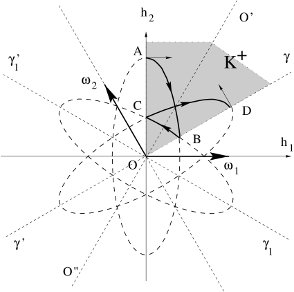
Figure 4: Classical dynamics in the Weyl chamber of SU(3)

Within the path integral formalism for the model, we shall see that the phase of the wave function does not change under such a reflection, in full contrast with the realistic reflection from an infinite potential wall where the phase would be shifted by $\pi$.

At the point $C$ the oscillator hits the boundary of the Weyl chamber one more time and follows the elliptic segment $C\rightarrow D$. Again, at the very moment of the collision, no abrupt change of the physical state occurs. Finally, at $t=\pi$ the oscillator reaches the point $D$, reflects from the boundary and goes the same way back to the point $A$, returning there at $t=2\pi$.

What are independent frequencies of this two-dimensional isotropic oscillator? It is quite surprising that they do not equal just one (the frequency that enters into the Hamiltonian), but rather 2 and $\nu=3$. By definition the angular frequency is $2\pi/T$ where $T$ is the time in which the system returns into the initial state upon periodic motion. The system state is specified by values of the momentum and position of the physical degree of freedom in question. Let us decompose the motion of the system into oscillations along the axis $O^{\prime}O^{\prime\prime}$ and the angular motion about the origin $O$. After passing the segments $A\rightarrow B\rightarrow C$ by the oscillator, the angular variable attains its initial value since the angles $O^{\prime}OC$ and $O^{\prime}OA$ coincide, while the equality of the corresponding (angular) canonical momentum at the points $A$ and $C$ follows from its conservation law. The angular degree of freedom returns to the initial state two more times as the oscillator follows the path $C\rightarrow D\rightarrow C$, and then returns to the initial state after passing the segments $C\rightarrow B\rightarrow A$. Thus, the period of the angular variable is three times less than that of the angular variable of an ordinary two-dimensional isotropic oscillator, i.e., the physical frequency is tripled. From Fig. 4 one can easily see that the states of the radial degree of freedom at points $A$ and $D$ are the same, so the physical frequency of the radial degree of freedom is doubled.

A similar analysis can also be done for the groups SO(5) $\sim$ Sp(4) and G₂. For them the independent frequencies appear to be $2$ and $\nu$. Note that the Weyl chamber is a sector with angle $\pi/\nu$. The numbers 2 and $\nu$ are, in fact, fine characteristics of the groups, namely, they are degrees of two independent invariant (Casimir) polynomials, which are ${\rm tr}\,x^{2}$ and ${\rm tr}\,x^{\nu}$ in a matrix representation. Any regular function $f(x)$ invariant under the adjoint action of the group on its argument is a function of these two independent polynomials. This fact holds for an arbitrary semisimple compact gauge group G: The independent frequencies of the isotropic harmonic oscillator are determined by degrees of independent Casimir polynomials. The number of the independent Casimir polynomials equals the rank of the group G, i.e., the number of physical degrees of freedom. The list of degrees of the independent Casimir polynomials for each group can be found in [32]. In the next subsection we shall develop a Hamiltonian formalism in explicitly gauge invariant variables and see the relation between the physical frequencies and orders of the independent Casimir polynomials once again.

So, in the classical theory the hyperconic structure of the physical phase space reveals itself through the effect of reflections of physical trajectories from the boundaries of the physical configuration space when the latter is parameterized by elements of the Cartan subalgebra. One should stress again that the effect of changing the physical frequencies of the oscillator does not depend on the choice of local canonical variables and is essentially due to the hyperconic structure of the physical phase space. To calculate the effect, we used the above parameterization of the physical phase space. The choice of the parameterization is, in fact, a matter of convenience. Had we taken another set of local canonical coordinates, say, by making cuts of the hyperconic phase space such that the momentum variable $p_{h}$ is restricted to the Weyl chamber, we would have arrived to the very same conclusion about the oscillator frequencies. The message is therefore: Whatever local canonical coordinates are assumed, the coordinate singularities associated with them should be carefully taken into account when solving the dynamical problem because they may contain information about the geometry of the physical phase space.

Another important observation is that the geometry of the physical phase space does not permit excitations of the Cartesian degrees of freedom $h^{i}$ independently, even though the Hamiltonian does not contain any interaction between them. This effect can be anticipated from the fact that the residual Weyl transformations mix the $h^{i}$. Such a kinematic coupling between the physical degrees of freedom appears to be crucial for constructing a correct path integral formalism for gauge systems [19, 18]. If the Hamiltonian does not contain any coupling between the degrees of freedom, then the transition amplitude in quantum mechanics is factorized over the degrees of freedom. This, however, is not the case if the phase space is not Euclidean. It can already be seen from the correspondence principle. Let us, for example, set $V=0$ in the above model. In addition to the straight trajectory connecting the initial point $h_{1}\in K^{+}$ and the final point $h_{2}\in K^{+}$, there are $2\nu-1$ trajectories which involve several reflections from the boundary of the Weyl chamber. Since no change of the physical state occurs at the very moment of the reflection, these trajectories would also be acceptable classical trajectories contributing to the semiclassical transition amplitude at the same footing as the straight one. The reflected trajectories can be viewed as straight lines connecting the points $\hat{R}h_{1},\ \hat{R}\in W$, and $h_{2}$. Hence, they satisfy the classical equations of motion. Using the Weyl symmetry they can be mapped into piecewise straight continuous trajectories inside of the Weyl chamber. The contribution of these trajectories makes it impossible to factorize the semiclassical transition amplitude because the reflected trajectories cannot be associated with an excitation of any particular Cartesian degrees of freedom $h^{i}$ (see Fig. 9 in section 8.5).

4.6 Gauge invariant canonical variables for groups of rank 2.

The analysis of classical dynamics of the isotropic harmonic oscillator shows that independent excitations of the Cartesian degrees of freedom $h^{1}$ and $h^{2}$ are impossible due to the non-Euclidean structure of their physical phase space. If, say, $p_{h2}=\dot{h}^{2}=0$ in the initial moment of time, then after hitting the boundary of the Weyl chamber, the momentum $p_{h1}=\dot{h}^{1}$ will be re-distributed between both physical degrees of freedom, thus exciting the $h^{2}$-degree of freedom. This occurs not due to an action of any local potential force (it can even be zero), but rather due to the non-Euclidean structure of the physical phase space. This specific kinematic coupling implies that the independent physical excitations must be collective excitations of the original degrees of freedom. Here we show that the collective excitations are described by composite gauge invariant variables. The goal is therefore to demonstrate that the kinematic coupling is important to maintain the gauge invariance of the Hamiltonian dynamics of physical canonical variables.

In the Hamiltonian (4.27) for groups of rank $r=2$ we introduce new gauge invariant variables [18]

$$\Phi_{1}=({\rm tr}\,x^{2})^{1/2}\ ,\ \ \ \ \Phi_{2}=\Phi_{1}^{-\nu}{\rm tr}\,x^{\nu}\ ,$$ (4.33)

where $\nu$ is the degree of the second independent Casimir polynomial. The use of a matrix representation is just a matter of technical convenience. The invariant independent (Casimir) polynomials can also be written via symmetric invariant irreducible tensors, ${\rm tr}\,x^{2}\sim\delta_{ab}x^{a}x^{b}$ and ${\rm tr}\,x^{\nu}\sim d^{(\nu)}_{a_{1}\cdots a_{\nu}}x^{a_{1}}\cdots x^{a_{\nu}}$. Every symmetric invariant tensor in a Lie algebra can be decomposed over the basis formed by irreducible symmetric invariant tensors [32]. Ranks of the irreducible tensors are orders of independent Casimir polynomials in the Lie algebra. The canonical momenta conjugate to the new variables read

$$\pi_{i}=\frac{{\rm tr}\,(pe_{i})}{{\rm tr}\,e_{i}^{2}}\ ,\ \ \ i=1,2\ ;\ \ \ e_{i}=\frac{\partial\Phi_{i}}{\partial x^{a}}\,\lambda_{a}\equiv\frac{\partial\Phi_{i}}{\partial x}\ .$$ (4.34)

By straightforward computation one can convince oneself that the elements $e_{i}$ possess the following properties:

$${\rm tr}\,(e_{1}e_{2})=0\ ,\ \ \ \ [e_{1},e_{2}]=0\ .$$ (4.35)

Therefore they can serve as the local basis in the Cartan subalgebra $H$. One can also show that

$${\rm tr}\,e_{1}^{2}=1\ ,\ \ {\rm tr}\,e_{2}^{2}=\frac{\nu^{2}}{\Phi_{1}^{2}}\,\left(c_{2}+c_{1}\Phi_{2}-\Phi_{2}^{2}\right)\equiv\frac{\nu^{2}}{\Phi_{1}^{2}}\,\left(a-\left[\Phi_{2}-b\right]^{2}\right)\,,\ \$$ (4.36)

where $b=c_{1}/2,\,a=c_{2}+c_{1}^{2}/4$, and the constants $c_{1,2}$ depend on the structure constants and specify the decomposition of the gauge invariant polynomial $[{\rm tr}\,(\lambda_{a}x^{\nu-1})]^{2}=(c_{1}\Phi_{2}+c_{2})\Phi_{1}^{2(\nu-1)}$ over the basis polynomials ${\rm tr}\,x^{2}$ and ${\rm tr}\,x^{\nu}$. For example, for SU(3) we have $\nu=3$ and $c_{1}=0$, $c_{2}=1/6$. This can be verified by a straightforward computation in the matrix representation.

Let us decompose the canonical momentum $p$ over the basis $e_{i}$, $p=\pi_{i}e_{i}+\tilde{p}$ where ${\rm tr}\,e_{i}\tilde{p}=0$. A solution to the constraint equation $[p,x]=[\tilde{p},x]=0$ is $\tilde{p}=0$. That is, all the components of $p$ orthogonal to the Cartan basis elements $e_{i}$ must vanish since the commutator of $\tilde{p}$ and $x\sim e_{1}$ does not belong to the Cartan subalgebra. The physical Hamiltonian of an isotropic harmonic oscillator, $V={\rm tr}\,x^{2}/2=\Phi_{1}^{2}/2$, assumes the form

$$H_{ph}=\frac{1}{2}\pi_{1}^{2}+\frac{\nu^{2}\pi_{2}^{2}}{2\Phi_{1}^{2}}\,\left(a-\left[b-\Phi_{2}\right]^{2}\right)+\frac{1}{2}\Phi_{1}^{2}\ .$$ (4.37)

From positivity of the norm ${\rm tr}\,e^{2}_{2}\geq 0$ we infer the condition

$$-1\leq(\Phi_{2}-b)/\sqrt{a}\leq 1\ .$$ (4.38)

The Hamiltonian equations of motion are

$$\dot{\pi}_{1} = \{\pi_{1},H_{ph}\}=-\Phi_{1}+\frac{\nu^{2}\pi_{2}^{2}}{\Phi_{1}^{3}}\,\left(a-\left[b-\Phi_{2}\right]^{2}\right)\,,$$

$$\dot{\Phi}_{1} = \{\Phi_{1},H_{ph}\}=\pi_{1}\,;$$ (4.39)

$$\dot{\pi}_{2} = \{\pi_{2},H_{ph}\}=\frac{\nu^{2}\pi_{2}^{2}}{\Phi_{1}^{2}}\,\left[b-\Phi_{2}\right]\,,$$

$$\dot{\Phi}_{2} = \{\Phi_{2},H_{ph}\}=\frac{\nu^{2}\pi_{2}}{\Phi_{1}^{2}}\,\left(a-\left[b-\Phi_{2}\right]^{2}\right)\,.$$ (4.40)

They admit the following oscillating solutions independently for each degree of freedom

$$\Phi_{2}(t) = \pi_{2}(t)=0\,;$$ (4.41)

$$\Phi_{1}(t) = \sqrt{E}|\cos t|\,,\ \ \ \pi_{1}(t)=-\sqrt{E}\sin t\,\varepsilon(\cos t)\ ,$$ (4.42)

where $E$ is the energy and $\varepsilon$ denotes the sign function; and

$$\Phi_{1}(t) = \sqrt{E}\ ,\ \ \ \ \ \ \ \ \pi_{1}(t)=0\ ;$$ (4.43)

$$\Phi_{2}(t) = b+\sqrt{a}\cos\nu t\ ,\ \ \ \pi_{2}(t)=-\frac{E}{\nu\sqrt{a}\sin{\nu t}}\ .$$ (4.44)

Absolute value bars in (4.42) are necessary because $\Phi_{1}$ is positive. One can easily see that the independent frequencies are degrees of the independent Casimir polynomials, 2 and $\nu$. Clearly, the variable $\cos^{-1}[(\Phi_{2}-b)/\sqrt{a}]$ can be associated with the angular variable introduced in the previous section and $\Phi_{1}$ with the radial variable.

Thanks to the gauge invariance of the new variables $\Phi_{1,2}$ we may always set $x=h$ in (4.33) and $p=p_{h}$ in (4.34), thus establishing the canonical transformation between the two sets of canonical variables. The kinematic coupling between $\Phi_{1,2}$ is absent. However, to excite either of $\Phi_{1,2}$ independently, excitations of both Cartesian degrees of freedom $h_{1,2}$ are needed. Thus, the removal of the kinematic coupling is equivalent to restoration of the explicit gauge invariance. In sections 7.3 and 7.4 we show that this remarkable feature has an elegant group theoretical explanation based on the theorem of Chevalley. The mathematical fact is that, if one attempts to construct all polynomials of $h$ invariant relative to the Weyl group, which specify wave functions of the physical excitations of the harmonic oscillator, then one would find that all such polynomials are polynomials of the elementary ones ${\rm tr}\,h^{2}$ and ${\rm tr}\,h^{\nu}$ [32]. Since orders of the polynomials determines the energy levels of the harmonic oscillator, we anticipate that the spectrum must be of the form $2n_{1}+\nu n_{2}$, where $n_{1,2}$ are nonnegative integers.

Remark. The canonical variables (4.33) and (4.34), though being explicitly gauge invariant and describing independent physical excitations of the harmonic oscillator, can be regarded as just another possible set of the local canonical coordinates on the non-Euclidean physical phase space. As one can see from (4.42) and (4.44), there are singularities in the phase space trajectories in these variables too. One can actually find arguments similar to those given at the end section 3.2 to show that there are no canonical coordinates on the hyperconic phase space in which the phase space trajectories are free of singularities. The singularities can be removed by introducing a noncanonical symplectic structure on the physical phase space (cf. section 3.3 and see section 6.4 for a generalization).

4.7 Semiclassical quantization

Having chosen the set $h,p_{h}$ of local canonical variables to describe elementary excitations of physical degrees of freedom, we have found a specific kinematic coupling as a consequence of the non-Euclidean structure of the physical phase space. If now we proceed to quantize the system in these variables, it is natural to expect some effects caused by the kinematic coupling. Let us take a closer look on them.

The Bohr-Sommerfeld quantization rule is coordinate-free, i.e., invariant under canonical transformations. We take advantage of this property and go over to the new canonical variables $\Phi_{i},\pi_{i}$ from $p_{h},h$. Note that due to the gauge invariance of the new variables we can always replace $x$ and $p$ in (4.33) and (4.34) by $h$ and $p_{h}$, respectively. We have

$$W=\oint(p_{h},dh)=\oint\left(\pi_{1}d\Phi_{1}+\pi_{2}d\Phi_{2}\right)=2\pi\hbar n\ ,$$ (4.45)

where $n$ is a non-negative integer. Here we have also omitted the vacuum energy [15]. For an ordinary isotropic oscillator of unit frequency, one can find that $E=n\hbar=(n_{1}+n_{2})\hbar$, where $n_{1,2}$ are non-negative integers, just by applying the rule (4.45) for an independent periodic motion of each degree of freedom. That is, the functional $W$ is calculated for the motion of one degree of freedom of the energy $E$, while the motion of the other degree of freedom is suppressed by an appropriate choice of the initial conditions. Then the same procedure applies to the other degree of freedom. So the total energy $E$ of the system is attained through exciting only one degree of freedom in the above procedure.

Although the independent excitations of the components of $h$ are impossible, the new canonical variables can be excited independently. Denoting $\oint\pi_{i}d\Phi_{i}=W_{i}(E)$ (no summation over $i$), we take the phase-space trajectory (4.42) and find

$$W(E)=W_{1}(E)=\pi E=2\pi\hbar n_{1}\ .$$ (4.46)

For the other degree of freedom we have the trajectory (4.44), which leads to

$$W(E)=W_{2}(E)=2\pi\nu^{-1}E=2\pi\hbar n_{2}\ .$$ (4.47)

Therefore we conclude that

$$E=\hbar(2n_{1}+\nu n_{2})\ .$$ (4.48)

Up to the ground state energy the spectrum coincides with the spectrum of two harmonic oscillators with frequencies $2$ and $\nu$, being degrees of the independent Casimir polynomials for groups of rank 2. We will see that the same conclusion follows from the Dirac quantization method for gauge systems without an explicit parameterization of the physical phase space.

4.8 Gauge matrix models. Curvature of the orbit space and the kinematic coupling

So far we have considered gauge models whose physical configuration space is flat. Here we give a few simple examples of gauge models with a curved gauge orbit space. Another purpose of considering these models is to elucidate the role of a non-Euclidean metric on the physical configuration space in the kinematic coupling between the physical degrees of freedom.

To begin with let us take a system of two particles in the plane with the Lagrangian being the sum of the Lagrangian (3.1), where $N=2$, [17, 16]

$$L=\frac{1}{2}\left(D_{t}{\bf x}_{1}\right)^{2}+\frac{1}{2}\left(D_{t}{\bf x}_{2}\right)^{2}+V_{1}({\bf x}_{1}^{2})+V_{2}({\bf x}_{2}^{2})\ ,$$ (4.49)

which is invariant under the gauge transformations

$${\bf x}_{q}\rightarrow e^{T\omega}{\bf x}_{q}\ ,\ \ \ \ y\rightarrow y+\dot{\omega}\ ,\ \ \ q=1,2\ .$$ (4.50)

The gauge transformations are simultaneous rotations of the vectors ${\bf x}_{1,2}$. By going over to the Hamiltonian formalism one easily finds that the system has two first-class constraints

$$\pi=\frac{\partial L}{\partial\dot{y}}=0\ ,\ \ \ \sigma=({\bf p}_{1},T{\bf x}_{1})+({\bf p}_{2},T{\bf x}_{2})=0\ .$$ (4.51)

The second constraint means that the physical motion has zero total angular momentum. The Hamiltonian of the system reads

$$H=\frac{1}{2}\left({\bf p}_{1}^{2}+{\bf p}_{2}^{2}\right)+V_{1}({\bf x}_{1}^{2})+V_{2}({\bf x}_{2}^{2})+y\sigma\equiv H_{1}+H_{2}\ ,$$ (4.52)

where each $H_{i}$ coincides with (3.21). The coupling between the degrees of freedom occurs only through the constraint.

The physical phase space of the system is the quotient ${\rm I\kern-1.79993ptR}^{2}\oplus{\rm I\kern-1.79993ptR}^{2}|_{\sigma=0}/SO(2)$ where the gauge transformations are simultaneous SO(2) rotations of all four vectors ${\bf x}_{q}$ and ${\bf p}_{q}$. To introduce a local parameterization of the physical phase by canonical coordinates, we observe that by a suitable gauge transformation the vector ${\bf x}_{1}$ can be directed along the first coordinate axis, i.e., $x_{1}^{(2)}=0$. Here we label the components of the vector ${\bf x}_{q}$ as $x_{q}^{(i)}$. So, the phase space of physical degrees of freedom can be determined by two conditions

$$x_{1}^{(2)}=0\ ,\ \ \ p_{1}^{(2)}=-\frac{1}{x_{1}^{(1)}}({\bf p}_{2},T{\bf x}_{2})\ .$$ (4.53)

The second equation follows from the constraint $\sigma=0$. The gauge condition still allows discrete gauge transformations generated by the rotations through the angles $n\pi$ ($n$ is an integer). It is important to understand that the residual gauge transformations on the hypersurface (4.53) do not act only on $p_{1}^{(1)}$ and $x_{1}^{(1)}$ changing their sign, but rather they apply to all degrees of freedom simultaneously: ${\bf x}_{q}\rightarrow\pm{\bf x}_{q}$ and ${\bf p}_{q}\rightarrow\pm{\bf p}_{q}$. The physical phase space cannot be split into a cone and two planes. It is isomorphic to the quotient

$${\rm PS}_{\rm phys}\sim{\rm I\kern-1.79993ptR}^{3}\oplus{\rm I\kern-1.79993ptR}^{3}/Z\!\!\!Z_{2}\ .$$ (4.54)

The residual gauge symmetry forbids independent excitations of the chosen canonical variables. Only pairwise excitations, like $x_{1}^{(1)}x_{2}^{(1)}$, are invariant under the residual gauge transformations. Thus, we have the familiar kinematic coupling of the physical degrees of freedom. Accordingly, if one takes the potentials $V_{1,2}$ as those of the harmonic oscillators, only pairwise collective excitations of the oscillators are allowed by the gauge symmetry, which is most easily seen in the Fock representation of the quantum theory (see section 7.1).

In addition to the kinematic coupling induced by the non-Euclidean structure of the physical phase space, there is another source for the kinematic coupling which often occurs in gauge theories. Making use of (4.23) we calculate the metric on the orbit space in the parameterization (4.53). Let us introduce a three-vector ${\bf q}$ whose components $q^{a}$, $a=1,2,3$, are, respectively, $x_{1}^{(1)}$, $x_{2}^{(1)}$, $x_{2}^{(2)}$. Then [17]

$$g^{ph}_{ab}=\frac{1}{{\bf q^{2}}}\left(\begin{array}[]{ccc}{\bf q}^{2}&0&0\\ 0&{\bf q}^{2}-(q^{3})^{2}&q^{3}q^{2}\\ 0&q^{3}q^{2}&{\bf q}^{2}-(q^{2})^{2}\end{array}\right)\ .$$ (4.55)

The metric (4.55) is not flat. The scalar curvature is $R=6/{\bf q}^{2}$. Since the metric is not diagonal, the reduction of the kinetic energy onto the physical phase space spanned by the chosen canonical variables will induce the coupling between physical degrees of freedom: ${\bf p}^{2}_{1}+{\bf p}^{2}_{2}=g_{ph}^{ab}p_{a}p_{b}$, where $p_{a}$ are canonical momenta for $q^{a}$. Thus, the physical Hamiltonian is no longer a sum of the Hamiltonians of each degree of freedom. The degrees of freedom described by ${\bf q}$ cannot be excited independently. It is possible to find new parameterization of the orbit space where the kinematic coupling caused by both the non-Euclidean structure of the phase space and the metric of the orbit space is absent [17] (the metric is diagonal in the new variables). The new variables are related to the ${\bf q}$’s by a non-linear transformation and naturally associated with the independent Casimir polynomials in the model (see section 7.1). In this regard, the model under consideration and the one discussed in section 4.5 are similar. So we will not go into technical details.

Let us calculate the induced volume element on the orbit space, $\mu({\bf q})d{\bf q}$. As before, the density $\mu({\bf q})$ does not coincide with $\sqrt{\det(g_{ab}^{ph})}=q^{1}/\sqrt{{\bf q}^{2}}$ because the volume of the gauge orbit through a configuration space point depends on that point [13]. Consider a matrix $x$ with the components $x_{ij}=x_{j}^{(i)}$, i.e., the columns of $x$ are vectors ${\bf x}_{j}$. Then the gauge transformation law is written in a simple form $x\rightarrow\exp(\omega T)x$. For this reason we will also refer to the model (4.49) as a gauge matrix model. For a generic point $x$ of the configuration space one can find a gauge transformation such that the transformed configuration satisfies the condition $x_{21}=0$. Therefore

$$x=e^{\theta T}\left(\begin{array}[]{cc}q^{1}&q^{2}\\ 0&q^{3}\end{array}\right)\equiv e^{\theta T}\rho\ ,$$ (4.56)

where the coordinates $q^{a}$ span the gauge orbit space. The volume element $\mu({\bf q})d{\bf q}d\theta$ can found by taking the square root of the determinant of the Euclidean metric ${\rm tr}\,(dx^{T}dx)={\rm tr}\,\{(d\rho+T\rho d\theta)^{T}(d\rho+T\rho d\theta)\}$, where $x^{T}$ is the transposed matrix $x$, in the new curvilinear coordinates. After a modest computation, similar to (4.21), we get the Jacobian $\mu({\bf q})=q^{1}$. Note that the variable ${\bf q}$ is gauge invariant in this approach, while $\theta$ spans the gauge orbits. We have ${\bf q}^{2}={\rm tr}\,(x^{T}x)$ and therefore the scalar curvature can also be written in the gauge invariant way $R=6/{\rm tr}\,(x^{T}x)$. Clearly, the curvature must be gauge invariant because it is a parameterization independent characteristic of the gauge orbit space.

The Jacobian $\mu$ vanishes at $q^{1}=0$. Its zeros form a plane in the space of $q^{a}$. On this plane the change of variables (4.56) is degenerate, which also indicates that the gauge $x_{21}=0$ is not complete on the plane $x_{11}=0$. Indeed, at the singular points $x_{11}=x_{1}^{(1)}=0$ the constraint cannot be solved for the nonphysical momentum $p_{1}^{(2)}$ and is reduced to $\sigma=({\bf x}_{2},T{\bf p}_{2})$ which generates the SO(2) continuous rotations on the plane ${\bf x}_{1}=0$. Such gauge transformations are known as the residual gauge transformations within the Gribov horizon [37, 99, 198]. Given a set of constraints $\sigma_{a}$ and the gauge conditions $\chi_{a}=0$ (such that $\{\chi_{a},\chi_{b}\}=0$ [67]), the Faddeev-Popov determinant is $\det\{\chi_{a},\sigma_{b}\}\equiv\Delta_{FP}$. Zeros of $\Delta_{FP}$ on the gauge fixing surface $\chi_{a}=0$ form the Gribov horizon (or horizons, if the set of zeros is disconnected). It has a codimension one (or higher) on the surface $\chi_{a}=0$. Within the Gribov horizon the gauge is not complete, and continuous gauge transformations may still be allowed [37]. Consequently, there are identifications within the Gribov horizon, which may, in general, lead to a nontrivial topology of the gauge orbit space [99] (see an example in section 10.3). In our case, $\chi=x_{1}^{(2)}$ and, hence, $\Delta_{FP}=x_{1}^{(1)}$, i.e., it coincides with the Jacobian $\mu$. This is a generic feature of gauge theories: The Faddeev-Popov determinant specifies the volume element on the gauge orbit space [13].

In our parameterization, the orbit space is isomorphic to the half-space $x_{1}^{(1)}>0$ modulo boundary identifications. To make the latter we can, e.g., make an additional gauge fixing on the plane $x_{1}^{(1)}=0$, say, by requiring $x_{2}^{(2)}=0$ [182]. We are left with discrete gauge transformations $x_{2}^{(1)}\rightarrow-x_{2}^{(1)}$. Therefore every half-plane formed by positive values of $x_{1}^{(1)}$ and values of $x_{2}^{(1)}$ would have the gauge equivalent half-axes $x_{2}^{(1)}>0$ and $x_{2}^{(1)}<0$ on its edge $x_{1}^{(1)}=0$. Identifying them we get the cone unfoldable into a half-plane. So the orbit space has no boundaries, and there is one singular point (the origin) where the curvature is infinite. The topology of the gauge orbit space is trivial.

On the Gribov horizon, the physical phase space of the model also exhibits the conic structure. On the horizon ${\bf x}_{1}=0$ the constraint is reduced to $\sigma=({\bf x}_{2},T{\bf p}_{2})$, so we get the familiar situation discussed in section 3.2: One particle on the plane with the gauge group SO(2). The corresponding physical phase space is a cone unfoldable into a half-plane, ${\rm I\kern-1.79993ptR}^{4}|_{\sigma=0}/SO(2)\sim cone(\pi)$.

Another interesting matrix gauge model can be obtained from the Yang-Mills theory under the condition that all vector potentials depend only on time [38, 39]. The orbit space in this model has been studied by Soloviev [37]. The analysis of the physical phase space structure and its effects on quantum theory can be found in [71, 10, 16]. The orbit space of several gauge matrix models is discussed in the work of Pause and Heinzl [182]. It is also noteworthy that gauge matrix models appear in the theory of eleven-dimensional supermembranes [40, 41], in the dynamics on D-particles [42] and in the matrix theory [43] describing some important properties of the superstring theory. The geometrical structure of the physical configuration and phase space of these models does not exhibit essentially new features. The details are easy to obtain by the method discussed above.

5 Yang-Mills theory in a cylindrical spacetime

The definition of the physical phase space as the quotient space of the constraint surface relative to the gauge group holds for gauge field theories, i.e., for systems with an infinite number of degrees of freedom. The phase space in a field theory is a functional space, and this gives rise to considerable technical difficulties when calculating the quotient space. One has to specify a functional class to which elements of the phase space, being a pair of functions of the spatial variables, belong. In classical theory it can be a space of smooth functions [12] (e.g., to make the energy functional finite). However, in quantum field theory the corresponding quotient space appears to be of no use, say, in the path integral formalism because the support of the path integral measure typically lies in a Sobolev functional class [44, 45, 34], i.e., in the space of distributions, where smooth classical configuration form a zero-measure subset. To circumvent this apparent difficulty, one can, for instance, discretize the space or compactify it into a torus (and truncate the number of Fourier modes), thus making the number of degrees of freedom finite. This would make a gauge field model looking more like mechanical models considered above where the quotient space can be calculated.

The simplest example of this type is the Yang-Mills theory on a cylindrical spacetime (space is compactified to a circle ${\bf S}^{1}$) [46, 47, 48, 49, 50, 51, 52, 53, 54]. Note that in two dimensional spacetime Yang-Mills theory does not have physical degrees of freedom, unless the spacetime has a nontrivial topology [55, 56, 57, 58, 59, 60, 61]. In the Hamiltonian approach, only space is compactified, thus leading to a cylindrical spacetime. We shall establish the ${\rm PS}_{{\rm phys}}$ structure of this theory in the case of an arbitrary compact semisimple gauge group [52, 54]. The Lagrangian reads

$$L=-\frac{1}{4}\int_{0}^{2\pi l}dx(F_{\mu\nu},F^{\mu\nu})\equiv-\frac{1}{4}\langle F_{\mu\nu},F^{\mu\nu}\rangle\ ,$$ (5.1)

where $F_{\mu\nu}=\partial_{\mu}A_{\nu}-\partial_{\nu}A_{\mu}-ig[A_{\mu},A_{\nu}],\ g$ a coupling constant, $\mu,\nu=0,1$; the Yang-Mills potentials $A_{\mu}$, being elements of a Lie algebra $X$, are periodic functions of a spatial coordinate, $A_{\mu}(t,x+2\pi l)=A_{\mu}(t,x)$, i.e. $l$ is the space radius; the parenthesis $(,)$ in the integrand (5.1) stand for the invariant inner product in $X$. We assume it to be the Killing form introduced in section 3.2. In a matrix representation, one can always normalize it to be a trace. Since the vector potential is a periodic function in space, it can be decomposed into a Fourier series. The Fourier components of $A_{\mu}$ are regarded as independent (Cartesian) degrees of freedom in the theory.

To go over to the Hamiltonian formalism, we determine the canonical momenta $E_{\mu}=\delta L/\delta\dot{A}^{\mu}=F_{0\mu}$; the overdot denotes the time derivative. The momentum conjugated to $A_{0}$ vanishes, $E_{0}=0$, forming the primary constraints. The canonical Hamiltonian has the form

$$H=\langle E_{\mu},A^{\mu}\rangle-L=\langle E_{1},E_{1}\rangle/2-\langle A_{0},\sigma\rangle\ ,$$ (5.2)

where $\sigma=\nabla(A_{1})E_{1}$ with $\nabla(A_{1})=\partial_{1}-ig[A_{1},\ ]$ being the covariant derivative in the adjoint representation. The primary constraints must be satisfied during the time evolution. This yields the secondary constraints

$$\dot{E}_{0}=\{E_{0},H\}=\partial_{1}E_{1}-ig[A_{1},E_{1}]=\sigma=0\ ,$$ (5.3)

where the standard symplectic structure

$$\{A^{a\mu}(x),E_{\nu}^{b}(y)\}=\delta^{ab}\delta^{\mu}_{\nu}\delta(x-y)\ ,\ \ \ \ \ x,y\in{\bf S}^{1}\ ,$$ (5.4)

has been introduced, and the suffices $a,b$ refer to the adjoint representation of the Lie algebra. The constraints are in involution

$$\{\sigma_{a}(x),\sigma_{b}(y)\}=if_{ab}{}^{c}\delta(x-y)\sigma_{c}(x)\ ,\ \ \ \ \{\sigma_{a},H\}=-f_{ab}{}^{c}A_{0}^{b}\sigma_{c}\ ,$$ (5.5)

with $f_{ab}{}^{c}$ being the structure constants of $X$. There are no more constraints in the theory, and all constraints are of the first class.

The primary and secondary (first-class) constraints are independent generators of gauge transformations. As in the mechanical models, the primary constraints $E_{0}^{a}=0$ generate shifts of the Lagrange multipliers $A_{0}^{a}$, $\delta A_{0}^{a}(x)=\{A_{0}^{a},\langle\omega_{0},E_{0}\rangle\}=\omega_{0}^{a}(x)$, and leave the phase space variables $E_{\mu}^{a}$ and $A_{1}^{a}$ unchanged. Therefore the hyperplane $E_{0}^{a}=0$ ($E_{1}$ and $A_{1}$ are fixed) spanned by $A^{a}_{0}$ in the total phase space is the gauge orbit. We can discard $A^{a}_{0}$ and $E^{a}_{0}$ as pure nonphysical degrees of freedom and concentrate our attention on the remaining variables.

To simplify the notation, from now on we omit the Lorentz suffix “1” of the field variables, i.e., instead of $E_{1}$ and $A_{1}$ we write just $E$ and $A$. The constraints (5.3) generate the following gauge transformations

$$E\rightarrow\Omega E\Omega^{-1}=E^{\Omega}\ ,\ \ \ \ A\rightarrow\Omega A\Omega^{-1}+\frac{i}{g}\Omega\partial\Omega^{-1}=A^{\Omega}\ .$$ (5.6)

Here and below $\partial_{1}\equiv\partial$, while the overdot is used to denote the time derivative $\partial_{0}$; $\Omega=\Omega(x)$ takes its values in a semisimple compact group $G$ ($X$ is its Lie algebra). The gauge transformed variables $E^{\Omega}$ and $A^{\Omega}$ must also be periodic functions of $x$. This results in the periodicity of $\Omega$ modulo the center $Z_{G}$ of $G$

$$\Omega(x+2\pi l)=z\Omega(x)\ ,\ \ \ \ \ z\in Z_{G}\ .$$ (5.7)

Indeed, by definition an element $z$ from the center commutes with any element of $X$ and, therefore, $E^{\Omega}$ and $A^{\Omega}$ are invariant under the shift $x\rightarrow x+2\pi l$. The relation (5.7) is called a twisted boundary condition [62]. The twisted gauge transformations (i.e., satisfying (5.7) with $z\neq e$, $e$ a group unit) form distinct homotopy classes. Therefore they cannot be continuously deformed towards the identity. On the other hand, gauge transformations generated by the constraints (5.3) are homotopically trivial because they are built up by iterating the infinitesimal transformations [8]: $\delta E=\{E,\langle\omega,\sigma\rangle\}=ig[E,\omega]$ and $\delta A=\{A,\langle\omega,\sigma\rangle\}=-\nabla(A)\omega$ with $\omega$ being an $X$-valued periodic function of $x$. Thus, we are led to the following conclusion. When determining ${\rm PS}_{{\rm phys}}$ as the quotient space, one should restrict oneself by periodic (i.e. homotopically trivial) gauge transformations. Such transformations determine a mapping ${\bf S}^{1}\rightarrow G$. A collection of all such transformations is called a gauge group and will be denoted ${\cal G}$, while an abstract group $G$ is usually called a structure group of the gauge theory. Yet we shall see that quantum states annihilated by the operators of the constraints – these are the Dirac physical states – are not invariant under the twisted gauge transformations.

Consider a periodic function $f(x)$ taking its values in $X$. It is expanded into a Fourier series

$$f(x)=f_{0}+\sum\limits_{n=1}^{\infty}\left(f_{s,n}\sin\frac{nx}{l}+f_{c,n}\cos\frac{nx}{l}\right)\ .$$ (5.8)

We denote a space of functions (5.8) ${\cal F}$ and its finite dimensional subspace formed by constant functions ${\cal F}_{0}$ so that $A=A_{0}+\tilde{A}$, where $A_{0}\in{\cal F}_{0}$ and $\tilde{A}\in{\cal F}\ominus{\cal F}_{0}$. For a generic connection $A(x)$, there exists a periodic gauge element $\Omega(x)$ such that the gauge transformed connection $A^{\Omega}$ is homogeneous in space,

$$\partial A^{\Omega}=0\ .$$ (5.9)

This means that the Coulomb gauge fixing surface $\partial A=0$ intersects each gauge orbit at least once. To find $\Omega(x)$, we set

$$\omega=-\frac{i}{g}\Omega^{-1}\partial\Omega\in X$$ (5.10)

and, hence,

$$\Omega(x)={\rm P}\exp ig\int_{x}^{0}\omega(x^{\prime})dx^{\prime}\ .$$ (5.11)

The path-ordered exponential (5.11) is defined similarly to the time-ordered exponential in section 3.1. They differ only by the integration variables. After simple algebraic transformations, Eq. (5.9) can be written in the form

$$\nabla(A)\omega=\partial\omega-ig[A,\omega]=-\partial{A}\ ,$$ (5.12)

which has to be solved for the Lie algebra element $\omega(x)$. It is a linear nonhomogeneous differential equation of first order. So its general solution is a sum of a general solution of the corresponding homogeneous equation and a particular solution of the nonhomogeneous equation. Introducing the group element

$$U_{A}(x)={\rm P}\exp ig\int_{0}^{x}dx^{\prime}A(x^{\prime})\ ,$$ (5.13)

that has simple properties $\partial U_{A}=igAU_{A}$ and $\partial U^{-1}_{A}=-igU^{-1}_{A}A$, the general solution can be written as

$$\omega(x)=U_{A}(x)\omega_{0}U_{A}^{-1}(x)-A(x)\ .$$ (5.14)

The first term containing an arbitrary constant Lie algebra element $\omega_{0}$ represents a solution of the homogeneous equation, while the second term is obviously a particular solution of the nonhomogeneous equation. The constant $\omega_{0}$ should be chosen so that the group element (5.11) would satisfy the periodicity condition, which yields

$$\Omega(2\pi l)={\rm P}\exp ig\oint dx\,\omega=e\ ,$$ (5.15)

where $e$ is the group unit. This specifies completely the function $\omega(x)$, and, hence, $\Omega(x)$ for any generic $A(x)$. So, any configuration $A\in{\cal F}$ can be reduced towards a spatially homogeneous configuration by means of a gauge transformation.

Now we shall prove that the gauge reduction of $A$ to a homogeneous connection $A_{0}\in{\cal F}_{0}$ leads to a simultaneous gauge reduction of the momentum $E$ to $E_{0}\in{\cal F}_{0}$ on the constraint surface. To this end, we substitute the gauge transformed canonical pair $A^{\Omega}=A_{0}\in{\cal F}_{0}$, $E^{\Omega}$ into the constraint equation $\nabla(A)E=0$ and obtain

$$\nabla(A^{\Omega})E^{\Omega}=\nabla(A_{0})E^{\Omega}=0\ .$$ (5.16)

The momentum variable is then divided into a homogeneous part $E_{0}$ and a nonhomogeneous one $\tilde{E}^{\Omega}=E^{\Omega}-E_{0}$. For these two components one obtains two independent equations from Eq. (5.16):

$$\sigma_{0}\equiv[A_{0},E_{0}] = 0\ ,$$ (5.17)

$$\partial\tilde{E}^{\Omega}-ig[A_{0},\tilde{E}^{\Omega}] = \nabla(A_{0})\tilde{E}^{\Omega}=0\ .$$ (5.18)

The first equation stems from the ${\cal F}_{0}$-component of the constraint equation (5.16), while the second one is the constraint in the subspace ${\cal F}\ominus{\cal F}_{0}$. A general solution of Eq. (5.18) can written in the form $\tilde{E}^{\Omega}(x)=U_{0}(x)\tilde{E}^{\Omega}_{0}U_{0}^{-1}(x)$ where $U_{0}(x)=\exp[igA_{0}x]$ and $\partial\tilde{E}^{\Omega}_{0}=0$. For a generic $A_{0}$, the solution is not periodic in $x$ for all constants $\tilde{E}^{\Omega}_{0}\neq 0$. Since $\tilde{E}^{\Omega}(x)$ must be a periodic function, the constant $\tilde{E}^{\Omega}_{0}$ should necessarily vanish. Thus, Eq. (5.18) has only a trivial solution $\tilde{E}^{\Omega}=0$, and $E^{\Omega}=E_{0}\in{\cal F}_{0}$.

A useful observation following from the above analysis is that the operator $\nabla(A_{0})$ has no zero modes in the subspace ${\cal F}\ominus{\cal F}_{0}$ and, hence, is invertible. The determinant of the operator $\nabla(A_{0})$ restricted on ${\cal F}\ominus{\cal F}_{0}$ does not vanish. We shall calculate it later when studying the metric on the physical configuration space.

We are led to a redundant system with $N=\dim X$ degrees of freedom and the constraint (5.17) which generates homogeneous gauge transformations of the phase-space variables $A_{0}$ and $E_{0}$ ($\partial\Omega\equiv 0$) . This mechanical system has been studied in Section 3. The system is shown to have $r={\rm rank}\ X$ physical degrees of freedom which can be described by Cartan subalgebra components of $A_{0}$ and $E_{0}$. Since any element of $X$ can be represented in the form $A_{0}=\Omega_{A}a\Omega_{A}^{-1}$, $a$ an element of the Cartan subalgebra $H$, $\Omega_{A}\in G$, configurations $A_{0}$ and $a$ belong to the same gauge orbit. Moreover, a spatially homogeneous gauge transformation with $\Omega=\Omega_{A}^{-1}$ brings the momentum $E_{0}$ on the constraint surface (5.17) to the Cartan subalgebra. Indeed, from (5.17) we derive $[a,\Omega_{A}^{-1}E_{0}\Omega_{A}]=0$ and conclude that $p_{a}=\Omega_{A}^{-1}E_{0}\Omega_{A}\in H$ by the definition of $H$. The element $a$ has a stationary group being the Cartan subgroup of $G$. This means that not all of the constraints (5.17) are independent. There are just $N-r,\ r=\dim H$, independent constraints among (5.17). The continuous gauge arbitrariness is exhausted in the theory.

5.1 The moduli space

We expect the existence of the residual gauge freedom which cannot decrease the number of physical degrees of freedom, but might change the geometry of their configuration and phase spaces. If two homogeneous connections from the Cartan subalgebra, $a$ and $a_{s}$, belong to the same gauge orbit, then there should exists a gauge group element $\Omega_{s}(x)$ such that

$$a_{s}=\Omega_{s}a\Omega_{s}^{-1}-\frac{i}{g}\Omega_{s}\partial\Omega_{s}^{-1}\ ,\ \ \ \partial a_{s}=\partial a=0\ ,\ \ \ a_{s},a\in H\ .$$ (5.19)

There are two types of solutions to this equation for $\Omega_{s}$. First, we can take homogeneous gauge group elements, $\partial\Omega_{s}=0$. This problem has already been solved in Section 3. The homogeneous residual gauge transformations form the Weyl group. Thus, we conclude that the phase-space points $\hat{R}p_{a},\ \hat{R}a$, where $\hat{R}$ ranges over the Weyl group, are gauge equivalent and should be identified when calculating the quotient space ${\rm PS}_{{\rm phys}}$. To specify the corresponding modular domain in the configuration space, we recall that the Weyl group acts simply transitively on the set of Weyl chambers [30], p.458. Any element of $H$ can be obtained from an element of the positive Weyl chamber $K^{+}$ ($a\in K^{+}$ if $(a,\omega)>0$, for all simple roots $\omega$) by a certain transformation from $W$. In other words, the Weyl chamber $K^{+}$ is isomorphic to the quotient $H/W$.

In contrast with the mechanical model of Section 3, the Weyl group does not cover the whole admissible discrete gauge arbitrariness in the 2D Yang-Mills theory. To find nonhomogeneous solutions to Eq. (5.19), we take the derivative of it, thus arriving at the equation

$$\partial\Omega_{s}a\Omega_{s}^{-1}+\Omega_{s}a\partial\Omega_{s}^{-1}-\frac{i}{g}\partial\left(\Omega_{s}\partial\Omega_{s}^{-1}\right)=0\ .$$ (5.20)

To solve this equation, we introduce an auxiliary Lie algebra element $\omega_{s}=-\frac{i}{g}\Omega_{s}^{-1}\partial\Omega_{s}$. From (5.20) we infer that it satisfies the equation

$$\nabla(a)\omega_{s}=0\ .$$ (5.21)

For a generic $a$ from the Cartan subalgebra this equation has only a homogeneous solution which we write in the form

$$\omega_{s}=a_{0}\eta\ ,\ \ \ a_{0}=(gl)^{-1}\ ,\ \ \ \eta\in H\ .$$ (5.22)

Note that Eq.(5.21) can always be transformed into two independent equations by setting $\omega_{s}=a_{0}\eta+\tilde{\omega}_{s}$, where $\eta\in{\cal F}_{0}$ and $\tilde{\omega}_{s}\in{\cal F}\ominus{\cal F}_{0}$. As has been shown above, the operator $\nabla(A_{0})$ has no zero modes in the space ${\cal F}\ominus{\cal F}_{0}$, and, hence, so does $\nabla(a)=\Omega_{A}^{-1}\nabla(A_{0})\Omega_{A}$ which means that $\det\nabla(a)=\det\nabla(A_{0})\neq 0$. So $\tilde{\omega}_{s}=0$, whereas the homogeneous component satisfies the equation $\nabla(a)\eta=-ig[a,\eta]=0$, that is, $\eta$ must be from the Cartan subalgebra because it commutes with a generic $a$. From the relation $\partial\Omega_{s}=ig\Omega_{s}\omega_{s}$ we find that

$$\Omega_{s}(x)=\exp\left(iga_{0}\eta x\right)\ .$$ (5.23)

This is still not the whole story because the group element we have found must to obey the periodicity condition otherwise it does not belong to the gauge group. The periodicity condition yields the restriction on the admissible values of $\eta$:

$$\Omega_{s}(2\pi l)=\exp(2\pi i\eta)=e\ ,$$ (5.24)

where $e$ stands for the group unit. The set of elements $\eta$ obeying this condition is called the unit lattice in the Cartan subalgebra [30], p.305. The nonhomogeneous residual gauge transformations do not change the canonical momentum $p_{a}$, since $[p_{a},\eta]=0$, and shift the canonical coordinate $a\rightarrow a+a_{0}\eta$, along the unit lattice in the Cartan subalgebra.

Consider a diagram $D(X)$ being a union of a finite number of families of equispaced hyperplanes in $H$ determined by $(\alpha,a)\in a_{0}Z\!\!\!Z,\ \alpha$ ranges over the root system and $Z\!\!\!Z$ stands for the set of all integers. Consider then a group $T_{e}$ of translations in $H$, $a\rightarrow a+a_{0}\eta,$ where $\eta$ belongs to the unit lattice. The group $T_{e}$ leaves the diagram $D(X)$ invariant [30], p.305. The diagram $D(X)$ is also invariant with respect to Weyl group transformations. Since $W$ is generated by the reflections (4.19) in the hyperplanes orthogonal to simple roots, it is sufficient to prove the invariance of $D(X)$ under them. We have $(\alpha,\hat{R}_{\omega}a)=a_{0}n_{\omega}$ where $n_{\omega}=n-2k_{\omega}(\omega,\alpha)/(\omega,\omega)$ is an integer as $(a,\omega)=k_{\omega}a_{0},\ k_{\omega}\in Z\!\!\!Z$ because $a\in D(X)$. We recall that any root $\alpha$ can be decomposed over the basis formed by simple roots. The coefficients of this decomposition are all either nonnegative or nonpositive integers. Therefore the number $-2(\omega,\alpha)/(\omega,\omega)$ is a sum of integers since the elements of the Cartan matrix $-2(\omega,\omega^{\prime})/(\omega,\omega)$ are integers. So, $\hat{R}_{\omega}D(X)=D(X)$. Now we take the complement $H\ominus D(X)$. It consists of equal polyhedrons whose walls form the diagram $D(X)$. Each polyhedron is called a cell. A cell inside of the positive Weyl chamber $K^{+}$ such that its closure contains the origin is called the Weyl cell $K_{W}^{+}$.

The Weyl cell will play an important role in the subsequent analysis, so we turn to examples before studying the problem in general. The diagram $D(su(2))$ consists of points $na_{0}\omega/(\omega,\omega),\ n\in Z\!\!\!Z$ with $\omega$ being the only positive root of $su(2)$, $(\omega,\omega)=1/2$ ($\omega=\tau_{3}/4$ in the matrix representation). A cell of $H_{su(2)}\ominus D(su(2))$ is an open interval between two neighbor points of $D(su(2))$. Assuming the orthonormal basis in the Cartan subalgebra, we can write $a=\sqrt{2}a_{3}\omega,\ (a,a)=a_{3}^{2}$. Since the Weyl chamber $K^{+}$ is isomorphic to the positive half-line ${\rm I\kern-1.79993ptR}^{+}$, we conclude that $a$ belongs to the Weyl cell $K^{+}_{W}$ if $a_{3}$ lies in the open interval $(0,\sqrt{2}a_{0})$. The translations $a\rightarrow a+2na_{0}\omega/(\omega,\omega),\ n\in Z\!\!\!Z$, form the group $T_{e}$, and $W=Z\!\!\!Z_{2},\ \hat{R}_{\omega}a=-a$. Thus, $D(su(2))$ is invariant under translations from $T_{e}$ and the reflection from the Weyl group $W$.

For $X=su(3)$ we have three positive roots, $\omega_{1},\ \omega_{2}$ and $\omega_{12}=\omega_{1}+\omega_{2}$ which have the same norms.

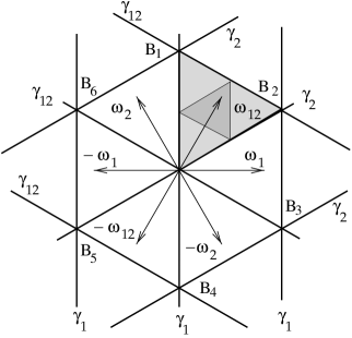
Figure 5: The root pattern of SU(3). The diagram $D(su(3))$ is formed by three families of straight lines perpendicular to the simple roots $\omega_{1},\omega_{2}$ and the root $\omega_{12}=\omega_{1}+\omega_{2}$. These families are denoted as $\gamma_{1},\gamma_{2}$ and $\gamma_{12}$, respectively. The grayed equilateral triangle is the Weyl cell of su(3) which is the moduli space of the su(3) connections with respect to homotopically trivial gauge transformations. Had we included the homotopically nontrivial transformations into the gauge group, the moduli space would have been four times less and isomorphic to the equilateral triangle whose vertices are the mid-points of the Weyl cell boundaries (see section 7.6 for details).

The angle between any two neighbor roots equals $\pi/3$. The root pattern of SU(3) is plotted in Fig. 5. The diagram $D(su(3))$ consists of three families of equispaced straight lines $(\omega_{1,2,12},a)=a_{0}n_{1,2,12},\ n\in Z\!\!\!Z$, on the plane $H_{su(3)}\sim{\rm I\kern-1.79993ptR}^{2}$. The lines are perpendicular to the roots $\omega_{1,2,12}$, respectively. The complement $H_{su(3)}\ominus D(su(3))$ is a set of equilateral triangles covering the plane $H_{su(3)}$. The Weyl cell $K^{+}_{W}$ is the triangle bounded by lines $(\omega_{1,2},a)=0$ (being the boundary of $K^{+}$) and $(\omega_{12},a)=a_{0}$. The group $T_{e}$ is generated by integral translations through the vectors $2a_{0}\alpha/(\alpha,\alpha),\ \alpha$ ranges over $\omega_{1,2,12}$, and $(\alpha,\alpha)=1/3$ (see section 3.2 for details of the matrix representation of the roots).

Let $W_{A}$ denote the group of linear transformations of $H$ generated by the reflections in all the hyperplanes in the diagram $D(X)$. This group is called the affine Weyl group [30], p.314. $W_{A}$ preserves $D(X)$ and, hence,

$$K^{+}_{W}\sim H/W_{A}\ ,$$ (5.25)

i.e. the Weyl cell is isomorphic to a quotient of the Cartan subalgebra by the affine Weyl group. Consider a group $T_{r}$ of translations

$$a\rightarrow a+2a_{0}\sum_{\alpha>0}n_{\alpha}\alpha/(\alpha,\alpha)\equiv a+a_{0}\sum_{\alpha>0}n_{\alpha}\eta_{\alpha},\ \ \ \ \ n_{\alpha}\in Z\!\!\!Z\ .$$

Then $W_{A}$ is a semidirect product of $T_{r}$ and $W$ [30], p.315. For the element $\eta_{\alpha}$ we have the following equality [30], p.317,

$$\exp(2\pi i\eta_{\alpha})=\exp\frac{4\pi i\alpha}{(\alpha,\alpha)}=e\ ,$$ (5.26)

Comparing it with (5.24) we conclude that the residual discrete gauge transformations form the affine Weyl group.

The space of all periodic connections $A(x)$ is ${\cal F}$. Now we can calculate the moduli space of connections relative to the gauge group, i.e., obtain the physical configuration space, or the gauge orbit space

$${\rm CS}_{{\rm phys}}={\cal F}/{\cal G}\sim H/W_{A}\sim K^{+}_{W}\ .$$ (5.27)

Similarly, the original phase space is ${\cal F}\oplus{\cal F}$ because it is formed by pairs of Lie-algebra-valued periodic functions $A(x)$ and $E(x)$. The quotient with respect to the gauge group reads

$${\rm PS}_{{\rm phys}}={\cal F}\oplus{\cal F}/{\cal G}\sim{\rm I\kern-1.79993ptR}^{2r}/W_{A}\ ,$$ (5.28)

where the action of $W_{A}$ on $H\oplus H\sim{\rm I\kern-1.79993ptR}^{2r}$ is determined by all possible compositions of the following transformations

$$\hat{R}_{\alpha,n}p_{a} = \hat{R}_{\alpha}p_{a}=p_{a}-\frac{2(\alpha,p_{a})}{(\alpha,\alpha)}\,\alpha\ ,$$ (5.29)

$$\hat{R}_{\alpha,n}a = \hat{R}_{\alpha}a+\frac{2n_{\alpha}a_{0}}{(\alpha,\alpha)}\,\alpha\ ,$$ (5.30)

where the element $\hat{R}_{\alpha,n}\in W_{A}$ acts on $a$ as a reflection in the hyperplane $(\alpha,a)=n_{\alpha}a_{0},\ n_{\alpha}\in Z\!\!\!Z$, and $\alpha$ is any root.

To illustrate the formula (5.28), let us construct ${\rm PS}_{{\rm phys}}$ for the simplest case $X=su(2)$. We have $r=1,\ W=Z\!\!\!Z_{2},\ (\omega,\omega)=1/2$.

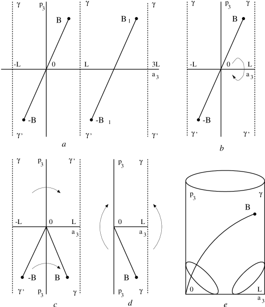
Figure 6: The physical phase space of the SU(2) Yang-Mills theory on a cylindrical spacetime. It is a half-cylinder with two conic horns attached to it. It is flat everywhere except the conic singularities where the curvature is infinite. Here $L=\sqrt{2}a_{0}$.

The group $T_{r}=T_{e}$ acts on the phase plane ${\rm I\kern-1.79993ptR}^{2}$ spanned by the coordinates $p_{3},a_{3}$ (we have introduced the orthonormal basis in $H_{su(2)}$; see the discussion of $D(su(2))$ above) as $p_{3},a_{3}\rightarrow p_{3},a_{3}+2\sqrt{2}na_{0}$. In Figure 6 we set $L=\sqrt{2}\,a_{0}$. The points $B$ and $B_{1}$ are related by the gauge transformation from $T_{e}$. The strips bounded by the vertical lines $(\gamma\gamma^{\prime})$ are gauge equivalent through the translations from $T_{e}$. The boundary lines $(\gamma\gamma^{\prime})$ are gauge equivalent to one another, too. So, ${\rm I\kern-1.79993ptR}^{2}/T_{e}$ is a cylinder. After an appropriate cut, this cylinder can be unfolded into the strip $p_{3}\in{\rm I\kern-1.79993ptR},\ a_{3}\in(-L,L)$ as shown in Fig. 6b. The boundary lines $a_{3}=\pm L$ are edges of the cut. They contain the same physical states and later will be identified. On the strip one should stick together the points $p_{3},a_{3}$ and $-p_{3},-a_{3}$ connected by the reflection from the Weyl group (the points $B$ and $-B$ in Fig. 6b). This converts the cylinder into a half-cylinder ended by two conic horns at the points $p_{3}=0,a_{3}=0,L$. Indeed, we can cut the strip along the $p_{3}$-line and rotate the right half (the strip $0<a_{3}<L$) relative to the coordinate axis $a_{3}$ through the angle $\pi$ (cf. a similar procedure in Fig. 1b). The result is shown in Fig. 6c. It is important to observe that the half-axis $(L\gamma)$ is gauge equivalent to $(-L\gamma)$ and $(-L\gamma^{\prime})$ to $(L\gamma^{\prime})$, while the positive and negative momentum half-axes in Fig. 6c are edges of the cut and therefore to be identified too (cf. Fig. 1c). Next, we fold the strip in Fig. 6c along the momentum axis to identify the points $B$ and $-B$. Finally, we glue together the half-lines $(\gamma L)$ with $(L\gamma)$ and $(p_{3}O)$ with $(Op_{3})$ in Fig. 6d, thus obtaining the physical phase space (Fig. 6e). In neighborhoods of the singular conic points, ${\rm PS}_{{\rm phys}}$ looks locally like $cone(\pi)$ studied in Section 2 because $W_{A}$ acts as the $Z\!\!\!Z_{2}$-reflections (5.29) and (5.30) with $\alpha=\omega$ and $n=0,1$ near $a_{3}=0,\sqrt{2}a_{0}$, respectively.

For groups of rank 2, all conic (singular) points of ${\rm PS}_{{\rm phys}}$ are concentrated on a triangle being the boundary $\partial K_{W}^{+}$ of the Weyl cell (if $X=su(3)$, $\partial K_{W}^{+}$ is an equilateral triangle with side length $\sqrt{3}a_{0}$ in the orthonormal basis defined in section 3.2). Let us introduce local symplectic coordinates $p_{a}^{\bot},\ a^{\bot}$ and $p_{a}^{\|},\ a^{\|}$ in a neighborhood of a point of $\partial K_{W}^{+}$ (except the triangle vertices) such that $a^{\bot}$ and $a^{\|}$ vary along lines perpendicular and parallel to $\partial K_{W}^{+}$, respectively. The $W_{A}$-reflection in the boundary of $\partial K^{+}_{W}$ going through this neighborhood leaves $p_{a}^{\|},\ a^{\|}$ invariant, while it changes the sign of the other symplectic pair, $p_{a}^{\bot},a^{\bot}\rightarrow-p_{a}^{\bot},-a^{\bot}$. Therefore ${\rm PS}_{{\rm phys}}$ locally coincides with ${\rm I\kern-1.79993ptR}^{2}\oplus cone(\pi)$. At the triangle vertices, two conic singularities going along two triangle edges merge. If those edges are perpendicular, ${\rm PS}_{{\rm phys}}$ is locally $cone(\pi)\oplus cone(\pi)$. If not, ${\rm PS}_{{\rm phys}}$ is a $4D-hypercone$. The tip of the $4D-hypercone$ is “sharper” than the tip of $cone(\pi)\oplus cone(\pi)$, meaning that the $4D-hypercone$ can be always put inside of $cone(\pi)\oplus cone(\pi)$ when the tips of both the hypercones are placed at the same point. Obviously, a lesser angle between the triangle edges corresponds to a “sharper” hypercone (cf. section 4.4).

A generalization of this pattern of singular points in ${\rm PS}_{{\rm phys}}$ to gauge groups of an arbitrary rank is trivial. The Weyl cell is an $rD$-polyhedron. ${\rm PS}_{{\rm phys}}$ has the most singular local $2rD-hypercone$ structure at the polyhedron vertices. On the polyhedron edges it is locally viewed as an ${\rm I\kern-1.79993ptR}^{2}\oplus 2(r-1)D-hypercone$. Then on the polyhedron faces, being polygons, the local ${\rm PS}_{{\rm phys}}$ structure is an ${\rm I\kern-1.79993ptR}^{4}\oplus 2(r-2)D-hypercone$, etc.

Remark. As in the mechanical models studied earlier one can choose various ways to parameterize the physical phase space. When calculating a quotient space, one can, for instance, restrict the values of the canonical momentum $E(x)$. This is equivalent to imposing a gauge condition on the field variables rather than on the connection [68, 72]. By a gauge rotation $E$ can be brought to the Cartan subalgebra at each point $x$. So we set $E(x)=E_{H}(x)\in H$. Decomposing the connection $A$ into the Cartan component $A_{H}(x)$ and $\bar{A}(x)\in X\ominus H$, we find that the constraint $\nabla(A)E_{H}=0$ is equivalent to two independent constraints: $\partial E_{H}=0$ and $[\bar{A},E_{H}]=0$. These are two components of the original constraint in $H$ and $X\ominus H$, respectively. From the Cartan-Weyl commutation relations follows that $\bar{A}(x)=0$. The residual constraints $\partial E_{H}=0$ generate the gradient shifts of the corresponding canonical variables: $A_{H}\rightarrow A_{H}+\partial\omega$, where $\partial\omega$ is a periodic function of $x$. We have obtained the so called Abelian projection of the theory [72]. Therefore the physical degrees of freedom can again be described by the pair $E_{H}(x)=p_{a}$ and $A_{H}=a$. Now $p_{a}$ can be taken into the Weyl chamber by an appropriate Weyl transformation, while $a$ is determined modulo shifts on the periods of the group torus (the shifts along the group unit lattice). Note that we can take $\omega=\eta x$ since $\partial\omega=\eta$ is periodic as is any constant. The necessary restrictions on $\eta$ follow from the periodicity condition on the corresponding gauge group element. Thus, we have another parameterization of the same physical phase space such that $p_{a}\in K^{+}$ and $a\in H/T_{e}$, which, obviously, corresponds to another cut of the $rD$-hypercone. The quantum theory of some topological field models in the momentum representation has been studied in [73, 74, 75].

5.2 Geometry of the gauge orbit space

Let us find the metric and the induced volume element of the physical configuration space. They will be used in quantum mechanics of the Yang-Mills theory under consideration. It is useful to introduce the following decomposition of the functional space (5.8)

$${\cal F}=\sum\limits_{n=0}^{\infty}\oplus{\cal F}_{n}=\sum\limits_{n=0}^{\infty}\oplus({\cal F}_{n}^{H}\oplus\bar{\cal F}_{n})\ ,$$ (5.31)

where ${\cal F}_{0}$ is a space of constant Lie algebra-valued functions (the first term in the series (5.8)), ${\cal F}_{n},n\neq 0$, is a space of functions with the fixed $n$ in the sum (5.8). Each subspace ${\cal F}_{n}$ is finite-dimensional, $\dim{\cal F}_{0}=\dim X,\ \dim{\cal F}_{n}=2\dim X,n\neq 0$ (we recall that Lie algebra-valued functions are considered). Functions belonging to ${\cal F}_{n}^{H}$ take their values in the Cartan subalgebra $H$, while functions from $\bar{\cal F}_{n}$ take their values in $X\ominus H$. All subspaces introduced are orthogonal with respect to the scalar product $\langle,\rangle=\int_{0}^{2\pi l}dx(,)$.

From the above analysis of the moduli space of Yang-Mills connections follows a local parameterization of a generic connection

$$A=\Omega a\Omega^{-1}+ig^{-1}\Omega\partial\Omega^{-1}\ ,\ \ \ \partial a=0\ ,\ \ a\in H\ ,$$ (5.32)

where $\Omega\in{\cal G}/G_{H}$, and $G_{H}$ is the Cartan subgroup (the maximal Abelian subgroup of $G$) which is isomorphic to the stationary group of the homogeneous connection $a$. By definition the connection remains invariant under gauge transformations from its stationary group. Eq. (5.32) can be regarded as a change of variables in the functional space ${\cal F}$. In the new variables the functional differential $\delta A\in{\cal F}$ can be represented in the form

$$\delta A=\Omega\left(da-ig^{-1}\nabla(a)\delta w\right)\Omega^{-1}\ ,$$ (5.33)

where by the definition of the parameterization (5.32) $\delta a=da\in{\cal F}_{0}^{H}$ and $\delta w(x)=i\Omega^{-1}\delta\Omega\in{\cal F}\ominus{\cal F}_{0}^{H}$. Therefore the metric tensor reads

$$\langle\delta A,\delta A\rangle = 2\pi l(da,da)-g^{-2}\langle\delta w,\nabla^{2}(a)\delta w\rangle$$

$$\equiv (da,g_{aa}da)+\langle\delta w,g_{ww}\delta w\rangle\ .$$

Equality (5.2) results from (5.33) and the relation that $\langle da,\nabla(a)\delta w\rangle=$ $-\langle\nabla(a)da,\delta w\rangle=0$ which is due to $\partial da=0$ and $[da,a]=0$. The operator $\nabla(a)$ acts in the subspace ${\cal F}\ominus{\cal F}_{0}^{H}$. It has no zero mode in this subspace if $a\in K_{W}^{+}$ and, hence, is invertible. Its determinant is computed below. The metric tensor has the block-diagonal form. The physical block is proportional to the $r\times r$ unit matrix $g_{aa}=2\pi l$. For the nonphysical sector we have an infinite dimensional block represented by the kernel of the differential operator: $g_{ww}=-g^{-2}\nabla^{2}(a)$, and $g_{aw}=g_{wa}=0$. Taking the inverse of the $aa$-block of the inverse total metric, we find that the physical metric $g_{aa}^{ph}$ coincides with $g_{aa}$. That is, the physical configuration space is a flat manifold with (singular) boundaries. It has the structure of an orbifold [36].

To obtain the induced volume element, one has to calculate the Jacobian of the change of variables (5.32)

$$\int_{{\cal F}}\prod\limits_{x\in{S}^{1}}dA(x)\Phi = \int_{{\cal G}/G_{H}}\prod_{x}dw(x)\int_{K^{+}_{W}}daJ(a)\Phi\rightarrow\int_{K_{W}^{+}}da\kappa^{2}(a)\Phi\ ,$$ (5.35)

$$J^{2}(a) = \det g_{aa}\det g_{ww}=(2\pi l)^{r}\det\left[-g^{-2}\nabla^{2}(a)\right]\ .$$ (5.36)

Here $\Phi=\Phi(A)=\Phi(a)$ is a gauge invariant functional of $A$. The induced volume element does not coincide with the square root of the determinant of the induced metric on the orbit space. It contains an additional factor, $(\det g_{ww})^{1/2}$, being the volume of the gauge orbit through a generic configuration $A(x)=a$, in the full accordance with the general analysis given in [13] for Yang-Mills theories (see also section 10.1). Consider the orthogonal decomposition

$$\bar{\cal F}_{n}=\sum\limits_{\alpha>0}\oplus{\cal F}_{n}^{\alpha}\ ,$$ (5.37)

where ${\cal F}_{n}^{\alpha}$ contains only functions taking their values in the two-dimensional subspace $X_{\alpha}\oplus X_{-\alpha}$ of the Lie algebra $X$. The subspaces ${\cal F}^{H}_{n},\ {\cal F}^{\alpha}_{n}$ are invariant subspaces of the operator $\nabla(a)$, that is, $\nabla(a){\cal F}^{H}_{n}$ is a subspace of ${\cal F}^{H}_{n}$, and $\nabla(a){\cal F}^{\alpha}_{n}$ is a subspace of ${\cal F}^{\alpha}_{n}$. We conclude that the operator $\nabla(a)$ has a block-diagonal form in the decomposition (5.31) and (5.37). Indeed, we have $\nabla(a)=\partial-ig{\rm ad}\,{a}$, where ${\rm ad}\,{a}=[a,\ ]$ is the adjoint operator acting in $X$. The operator $\partial$ is diagonal in the algebra space, and its action does not change periods of functions, i.e. ${\cal F}^{H,\alpha}_{n}$ are its invariant spaces. Obviously, ${\rm ad}\,{a}{\cal F}^{H}_{n}=0$ and ${\rm ad}\,{a}{\cal F}^{\alpha}_{n}={\cal F}^{\alpha}_{n}$ if $(\alpha,a)\neq 0$ in accordance with the Cartan-Weyl commutation relation (4.11). Therefore an action of the operator $\nabla(a)$ on ${\cal F}\ominus{\cal F}^{H}_{0}$ is given by an infinite-dimensional, block-diagonal matrix. In the real basis $\lambda_{i}$ introduced after Eq. (4.16), its blocks have the form

$$\nabla^{H}_{n}(a) \equiv \nabla(a)|_{{}_{{\cal F}^{H}_{n}}}=\partial|_{{}_{{\cal F}^{H}_{n}}}=\left(\otimes\frac{n}{l}\varepsilon\right)^{r},\ \ n\neq 0,\ \ r={\rm rank}\,X,$$ (5.38)

$$\nabla^{\alpha}_{0}(a) \equiv \nabla(a)|_{{}_{{\cal F}^{\alpha}_{0}}}=-ig{\rm ad}\,{a}|_{{}_{{\cal F}^{\alpha}_{0}}}=g(a,\alpha)\varepsilon\ ,$$ (5.39)

$$\nabla^{\alpha}_{n}(a) \equiv \nabla(a)|_{{}_{{\cal F}^{\alpha}_{n}}}={\rm 1\kern-2.70004ptI}\otimes\frac{n}{l}\varepsilon+g(a,\alpha)\varepsilon\otimes{\rm 1\kern-2.70004ptI}\ ,$$ (5.40)

where $\varepsilon$ is a 2$\times$2 totally antisymmetric matrix, $\varepsilon_{ij}=-\varepsilon_{ji},\varepsilon_{12}=1$; and ${\rm 1\kern-2.70004ptI}$ is the $2\times 2$ unit matrix. In (5.40) the first components in the tensor products correspond to the algebra indices, while the second ones determine the action of $\nabla(a)$ on the functional basis $\sin(xn/l),\ \ \cos(nx/l)$. The vertical bars at the operators in Eqs. (5.38)–(5.40) mean a restriction of the corresponding operator onto a specified finite dimensional subspace of ${\cal F}$. An explicit matrix form of the restricted operator is easily obtained by applying $\partial$ to the Fourier basis, and the action of ${\rm ad}\,a$, $a\in H$, is computed by means of (4.15). Since $\varepsilon^{2}=-1$, we have for the Jacobian

$$J^{2}(a) = (2\pi l)^{r}\prod\limits_{\alpha>0}\det(ig^{-1}\nabla^{\alpha}_{0})^{2}\prod\limits_{n=1}^{\infty}\left[\det(ig^{-1}\nabla^{H}_{n})^{2}\prod\limits_{\alpha>0}\det(ig^{-1}\nabla^{\alpha}_{n})^{2}\right]=$$ (5.41)

$$= (2\pi l)^{r}\prod\limits_{\alpha>0}(a,\alpha)^{4}\prod\limits_{n=1}^{\infty}\left[\left(\frac{n}{gl}\right)^{4r}\prod\limits_{\alpha>0}\left(\frac{n^{2}}{g^{2}l^{2}}-(a,\alpha)^{2}\right)^{4}\right]\ .$$

Set $J(a)=C(l)\kappa^{2}(a)$. Including all divergences of the product (5.41) into $C(l)$ we get

$$\kappa(a) = \prod\limits_{\alpha>0}\left[\frac{\pi(a,\alpha)}{a_{0}}\prod\limits_{n=1}^{\infty}\left(1-\frac{(a,\alpha)^{2}}{a^{2}_{0}n^{2}}\right)\right]=\prod\limits_{\alpha>0}\sin\frac{\pi(a,\alpha)}{a_{0}}\ ,$$ (5.42)

$$C(l) = (2\pi l)^{r/2}\left(\frac{a_{0}}{\pi}\right)^{N_{+}}\prod\limits_{n=1}^{\infty}(n^{2}a_{0}^{2})^{r+2}\ ,$$ (5.43)

where $a_{0}=(gl)^{-1}$, the integer $N_{+}=(N-r)/2$ is the number of positive roots in $X$; the last equality in (5.42) results from a product formula given in [65], p.37. The induced volume element is $da\kappa^{2}(a)$. It vanishes at the boundaries of the Weyl cell (at the boundaries of the physical configuration space in the parameterization considered) since $(a,\alpha)/a_{0}\in Z\!\!\!Z$ for all $a\in\partial K_{W}^{+}$. Zeros of the function $\kappa(a)$ extended to the whole Cartan subalgebra form the diagram $D(X)$. This fact will be important for quantization of the model in section 8.6.

5.3 Properties of the measure on the gauge orbit space

We will need a few mathematical facts about the function $\kappa$ which are later proved to be useful when solving quantum Yang-Mills theory on a cylindrical spacetime in the operator and path integral approaches.

The first remarkable fact is that the function (5.42) is proportional to the Weyl determinant [63], p.185

$$(2i)^{N_{+}}\kappa(a) = \prod\limits_{\alpha>0}\left(e^{i\pi(a,\alpha)/a_{0}}-e^{-i\pi(a,\alpha)/a_{0}}\right)$$ (5.44)

$$= \sum\limits_{\hat{R}\in W}\det\hat{R}\exp\left[\frac{2\pi i}{a_{0}}(\hat{R}\rho,a)\right]\ .$$

Here we have introduced the parity $\det\hat{R}$ of the elements of the Weyl group. It is 1 if $\hat{R}$ contains even number of the generating elements $\hat{R}_{\omega}$ and $-1$ if this number is odd. Recall that in the root space ${\rm I\kern-1.79993ptR}^{r}$ the reflection $\hat{R}_{\omega}$ in the hyperplane orthogonal to a simple root $\vec{\omega}$ can be thought as an $r\times r$-matrix from the orthogonal group O($r$) such that $\det\hat{R}_{\omega}=-1$. The element $\rho$ is a half-sum of all positive roots:

$$\rho=\frac{1}{2}\sum\limits_{\alpha>0}\alpha\ .$$ (5.45)

The relation between $\kappa$ and the Weyl determinant allows us to establish the transformation properties of $\kappa$ relative to the action of the affine Weyl group on its argument. From (5.30) and (5.44) we infer

$$(2i)^{N_{+}}\kappa(\hat{R}_{\beta,n}a)$$ (5.46)

$$= \sum\limits_{\hat{R}\in W}\det\hat{R}\exp\left[\frac{2\pi i}{a_{0}}(\hat{R}\rho,\hat{R}_{\beta}a)\right]\exp\left[\frac{4\pi in_{\beta}}{(\beta,\beta)}\,(\hat{R}\rho,\beta)\right]$$

$$= \det\hat{R_{\beta}}\sum\limits_{\hat{R}\in W}\det\hat{R}\exp\left[\frac{2\pi i}{a_{0}}(\hat{R}\rho,a)\right]\exp\left[-\,\frac{4\pi in_{\beta}}{(\beta,\beta)}\,(\hat{R}\rho,\beta)\right]\ ,$$ (5.47)

where we have rearranged the sum over the Weyl group by the change $\hat{R}\rightarrow\hat{R}_{\beta}\hat{R}$ and made use of the properties that $\hat{R}_{\beta}^{2}=1$ and $\hat{R}_{\beta}\beta=-\beta$. Next we show that the second exponential in (5.47) is 1 for any $\beta$ and $\hat{R}$.

To this end, we observe that $(\hat{R}\rho,\beta)=(\rho,\beta^{\prime})$ where $\beta^{\prime}=\hat{R}^{T}\beta$ is also a root that has the same norm as $\beta$ because the Weyl group preserves the root pattern. Therefore we have to prove that

$$n_{\rho}(\beta)=\frac{2(\rho,\beta)}{(\beta,\beta)}$$ (5.48)

is an integer. The half-sum of the positive roots has the following properties [30], p.461,

$$\frac{2(\omega,\rho)}{(\omega,\omega)}=1\ ,$$ (5.49)

$$\hat{R}_{\omega}\rho=\rho-\omega\ ,$$ (5.50)

for any simple root $\omega$. Since the Weyl group $W$ preserves the root system and the reflection $\hat{R}_{\beta}$ in the hyperplane $(\beta,a)=0$ is a composition of reflections $\hat{R}_{\omega}$, there exists an element $\hat{R}\in W$ and a simple root $\omega_{\beta}$ such that $\hat{R}\omega_{\beta}=\beta$. The statement that $n_{\rho}(\beta)$ is an integer follows from the relation

$$n_{\rho}(\beta)=\frac{2(\beta,\rho)}{(\beta,\beta)}=\frac{2(\omega_{\beta},\hat{R}^{T}\rho)}{(\omega_{\beta},\omega_{\beta})}\in Z\!\!\!Z\ .$$ (5.51)

Indeed, representing $\hat{R}^{T}$ as a product of the generating elements $\hat{R}_{\omega}$ and applying (5.49) and (5.50) we obtain (5.51) from the fact that $2(\omega_{\beta},\alpha)/(\omega_{\beta},\omega_{\beta})$ is an integer for any root $\alpha$. Recall that a root $\alpha$ can be decomposed into a sum over simple roots with integer valued coefficients, and the Cartan matrix $2(\omega,\omega^{\prime})/(\omega,\omega)$ is also integer valued.

Thus, we arrive at the simple property

$$\kappa(\hat{R}_{\beta,n}a)=\det{\hat{R}_{\beta}}\,\kappa(a)=-\kappa(a)\$$ (5.52)

for any root $\beta$. Since any elements of the affine Weyl group $W_{A}$ is a composition of the reflections (5.30), we conclude that

$$\kappa(\hat{R}a)=\det{\hat{R}}\,\kappa(a)=\pm\kappa(a),\ \ \hat{R}\in W_{A}\ ,$$ (5.53)

where by definition $\det\hat{R}=-1$ if $\hat{R}$ contains an odd number of the reflections (5.30) and $\det\hat{R}=1$ for an even number. The Jacobian $\mu=\kappa^{2}$ is invariant under the affine Weyl group transformations.

The second remarkable property of the function $\kappa(a)$ is that it is an eigenfunction of the $r$–dimensional Laplace operator

$$(\partial_{a},\partial_{a})\kappa(a)\equiv\Delta_{(r)}\kappa(a)=-\frac{4\pi^{2}(\rho,\rho)}{a_{0}^{2}}\,\kappa(a)=-\frac{\pi^{2}N}{6a_{0}^{2}}\,\kappa(a)\ ,$$ (5.54)

where the relation $(\rho,\rho)=N/24$ [32] between the norm of $\rho$ and the dimension $N$ of the Lie algebra has been used. A straightforward calculation of the action of the Laplace operator on $\kappa(a)$ leads to the equality

$$\Delta_{(r)}\kappa(a)= - \frac{4\pi^{2}}{a_{0}^{2}}(\rho,\rho)\,\kappa(a)$$ (5.55)

$$+ \frac{\pi^{2}}{a_{0}^{2}}\sum\limits_{\alpha\neq\beta>0}(\alpha,\beta)\left[\cot\frac{\pi(a,\alpha)}{a_{0}}\cot\frac{\pi(a,\alpha)}{a_{0}}+1\right]\kappa(a)\ .$$

The sum over positive roots in (5.55) can be transformed into a sum over the roots $\alpha\neq\beta$ in a plane $P_{\alpha\beta}$ and the sum over all planes $P_{\alpha\beta}$. Each plane contains at least two positive roots. Relation (5.54) follows from

$${\sum\limits_{\alpha\neq\beta>0\in P_{\alpha\beta}}}(\alpha,\beta)[\cot(b,\alpha)\cot(b,\beta)+1]=0\ ,$$ (5.56)

for any $b\in H$. To prove the latter relation, we remark that the root pattern in each plane coincides with one of the root patterns for algebras of rank 2, su(3), sp(4)$\sim$ so(5) and g₂, because the absolute value of cosine of an angle between any two roots $\alpha$ and $\beta$ may take only four values $|\cos\theta_{\alpha\beta}|=\ 0,\ 1/\sqrt{2},\ 1/2,\ \sqrt{3}/2$. For the algebras of rank 2, equality (5.56) can be verified by an explicit calculation. For example, in the case of the su(3) algebra, the sum (5.56) is proportional to

$$-\cot b_{1}\cot b_{2}+\cot b_{1}\cot(b_{1}+b_{2})+\cot b_{2}\cot(b_{1}+b_{2})+1 = 0\ ,$$

where $b_{1,2}=(b,\omega_{1,2})$, and $\omega_{1},\omega_{2}$ and $\omega_{1}+\omega_{2}$ constitute all positive roots of SU(3).

6 Artifacts of gauge fixing in classical theory

The definition of ${\rm PS}_{{\rm phys}}$ is independent of the choice of local symplectic coordinates and explicitly gauge-invariant. However, upon a dynamical description (quantum or classical) of constrained systems, we often need to introduce coordinates on ${\rm PS}_{{\rm phys}}$, which means fixing a gauge or choosing a ${\rm PS}_{{\rm phys}}$ parameterization. The choice of the parameterization is usually motivated by physical reasons. If one deals with gauge fields, one may describe physical degrees of freedom by transverse components ${\bf A}^{\bot}$ of the vector potential and their canonically conjugated momenta ${\bf E}^{\bot}$, i.e. the Coulomb gauge $\partial_{i}A_{i}=0$ is imposed to remove nonphysical degrees of freedom. This choice comes naturally from our experience in QED where two independent polarizations of a photon are described by the transverse vector-potential. The Coulomb gauge is a complete global gauge condition in QED. Apparently, the phase space of each physical degree of freedom in the theory is a Euclidean space.

In the high-energy limit of non-Abelian gauge theories like QCD the physical picture of self-interacting transverse gluons works extremely well. However, in the infrared domain where the coupling constant becomes big and dynamics favors large fluctuations of the fields, transverse gauge fields do not serve any longer as good variables parameterizing ${\rm PS}_{{\rm phys}}$. It appears that there are gauge-equivalent configurations in the functional hyperplane $\partial_{i}A_{i}=0$, known as Gribov’s copies [11]. Moreover, this gauge fixing ambiguity always occurs and has an intrinsic geometric origin [12] related to the topology of the gauge orbit space and cannot be avoided if gauge potentials are assumed to vanish at spatial infinity. This makes a substantial difficulty for developing a consistent nonperturbative path integral formalism for gauge theories (see section 10 for details).

To illustrate the Gribov copying phenomenon in the Coulomb gauge, one can take the 2D Yang-Mills theory considered above. The spatially homogeneous Cartan subalgebra components of the vector potential $A=a$ and field strength $E=p_{a}$ can be regarded as symplectic coordinates on ${\rm PS}_{{\rm phys}}$. In fact, this implies the Coulomb gauge condition $\partial A=0$. This condition is not complete in the two-dimensional case because there are some nonphysical degrees of freedom left . They are removed by imposing an additional gauge condition $(e_{\pm\alpha},A)=0$, i.e. $A\in H$. Gribov copies of a configuration $A=a\in H\sim{\rm I\kern-1.79993ptR}^{r}$ are obtained by applying elements of the affine Weyl group $W_{A}$ to $a$. The modular domain coincides with the Weyl cell. By definition, the modular domain of the gauge fixing surface consists of configurations whose Gribov copies, if any, lie outside it. We will see that the residual transformations from the affine Weyl group are important for constructing the Hamiltonian path integral in the Coulomb gauge for the model in question. In fact, if we ignore them and calculate the path integral as if there were no Gribov copies, the answer would appear in conflict with the explicitly gauge invariant approach due to Dirac.

From the geometrical point of view [12], the absence of a “good” gauge condition $\chi({\bf A})=0$ is due to nontriviality of the fiber bundle with the base being space (compactified into a sphere by imposing zero boundary conditions on the connection ${\bf A}$ at the spatial infinity) and the fibers being the group G (see also a comprehensive work [167]). For this reason, the Gribov problem is often identified with the absence of the global cross-section on the non-trivial fiber bundle. However, one could look at this problem differently. Gribov found the obstruction to the nonperturbative extension of the Faddeev-Popov path integral [66]. To give an operator interpretation to the Lagrangian gauge-fixed (formal) path integral, a more general Hamiltonian path integral has been developed by Faddeev [67]. The construction is based on an explicit parameterization of the physical phase space, which is introduced by imposing supplementary (gauge) conditions on the canonical variables. We have discussed such parameterizations of the physical phase space in the SO(N) model (the gauge $x_{i}=x\delta_{1i}$), in the Yang-Mills mechanics (the gauge $x=h\in H$), or in the 2D Yang-Mills theory (the gauge $A(x)=a\in H$). The singularities discovered by Gribov are associated with the particular choice of the supplementary conditions imposed on the canonical coordinates (connections ${\bf A}$). In Yang-Mills theory this particular class of gauge conditions is indeed subject to the mathematical “no-go” theorem due to Singer. As has later been proposed by Faddeev with collaborators, this mathematical problem of constructing a cross-section on the non-trivial fiber bundle can be circumvented if the supplementary condition is imposed on the momentum variables [68]. One could even construct a set of local gauge invariant canonical variables to span the physical phase space [69, 70]. The gauge fixing in the space of the canonical momenta ${\bf E}$ is an algebraic (local) problem similar to the one discussed in section 3 because under the gauge transformations, ${\bf E}\rightarrow\Omega{\bf E}\Omega^{-1}$ [71].

The physical phase space structure does not depend whether one uses canonical coordinates or momenta to remove the gauge arbitrariness. The problem of constructing the correct path integral measure on the physical phase space parameterized in either way would still remain because there would be singularities in the canonical momentum space or in the configuration space as the consequence of the non-Euclidean structure of the physical phase space. ’t Hooft considered gauge fixing for the field variables rather than for the vector potentials [72]. He identified the singularities occurring in such a gauge with topological defects in gauge fields that carry quantum numbers of magnetic monopoles with respect to the residual Abelian gauge group. The existence of singularities in the momentum space were also stressed in [68].

In view of these arguments, we consider the Gribov obstruction as a part of a much more general and fundamental quantization problem: Quantization on non-Euclidean phase spaces. The phase space of physical degrees of freedom may not be Euclidean even if one can find a global cross section in the fiber bundle associated with a gauge model. In fact, it is the geometry of the phase space that lies at the heart of the canonical or path integral quantization because the Heisenberg commutation relations and their representation strongly depend on it. The quantization problem of non-Euclidean phase spaces is known since the birth of quantum mechanics. Yang-Mills theory has given us a first example of the fundamental theory where such an unusual feature of the Hamiltonian dynamics may have significant physical consequences.

An explicit parameterization of the physical phase space by local canonical coordinates is often used in gauge theories, e.g., in the path integral formalism. Although a particular set of canonical variables may look preferable from the physical point of view, it may not always appear reasonable from the mathematical point of view as a natural and convenient set of local canonical coordinates on a non-Euclidean phase space because it may create artificial (coordinate dependent) singularities in a dynamical description. On the other hand, it could also happen that the physical phase space is hard to compute and find mathematically most convenient coordinates to describe dynamics. Therefore it seems natural to take a closer look at possible “kinematic” effects caused by the coordinate singularities in a generic parameterization of the physical phase space. Here we investigate classical Hamiltonian dynamics. A quantum mechanical description will be developed in next section.

6.1 Gribov problem and the topology of gauge orbits

Gribov copies themselves do not have much physical meaning because they strongly depend on a concrete choice of a gauge fixing condition that is rather arbitrary. An “inappropriate” choice of the gauge condition can complicate a dynamical description. To illustrate what we mean by this statement, let us take a simple gauge model with three degrees of freedom whose dynamics is governed by the Lagrangian

$$L=\frac{1}{2}\dot{x}^{2}_{1}+\frac{1}{2}(\dot{x}_{2}-y)^{2}-V(x_{1})\ .$$ (6.1)

The Lagrangian is invariant under the gauge transformations $x_{2}\rightarrow x_{2}+\xi$, $y\rightarrow y+\dot{\xi}$, while the variable $x_{1}$ remains invariant. The variable $y$ is the Lagrange multiplier since the Lagrangian does not depend on the velocity $\dot{y}$. We can exclude it from consideration at the very beginning. On the plane spanned by the other two variables $x_{1,2}$, the gauge orbits are straight lines parallel to the $x_{2}$ axis. Therefore any straight line that is not parallel to the $x_{2}$ axis can serve as a unique gauge fixing condition because it intersects each orbit precisely once.

However, one is free to choose any gauge fixing condition, $\chi(x_{1},x_{2})=0$, to remove the gauge arbitrariness. A necessary condition on the gauge fixing curve is that it should intersect each gauge orbit at least once. In the dynamical description, this amounts to a specific choice of the function $y(t)$ in the Euler-Lagrange equations of motion. Recall that the equations of motion do not impose any restrictions on the Lagrange multipliers in gauge models because of their covariance under gauge transformations. Therefore the solutions depend on generic functions of time, the Lagrange multipliers, which can be specified so that the solutions would fulfill a supplementary (or gauge) condition. Now let us take the parametric equations of the gauge fixing curve $x_{1,2}=f_{1,2}(u)$ and let $u$ range over the real line. One can, for instance, set $f_{1,2}(0)=0$ and let $u$ equal the arc length of the curve counted in one direction from the origin and negative of the arc length, when the latter counted in the other direction traced out by the curve from the origin. The parameter $u$ describes the only physical degree of freedom in the model.

Figure 7: a). An illustration to an artificially created Gribov copying. The gauge fixing curve $AA^{\prime}$ intersects each gauge orbit, being vertical parallel straight lines, precisely once. There is a one-to-one correspondence between the parameter $u$ of the gauge fixing curve and the gauge invariant variable $x_{1}$. In contrast, the curve $\gamma\gamma^{\prime}$ does not intersect each gauge orbit once. The states labeled by the values of $u$ from the intervals $(u_{1},u_{2})$, $(u_{2},u_{3})$ and $(u_{3},u_{4})$ are gauge equivalent.Two of them must be discarded to achieve a unique parameterization of the gauge orbit space. If the first and third intervals are removed, then, in the $u$–parameterization, the configuration space would have two “holes”. There is no one-to-one correspondence between $u$ and $x_{1}$. In fact, the function $u(x_{1})$ is multi-valued and has, in this particular case, three branches.
b). Gribov problem in the SO(2) model. Here the gauge fixing curve $\chi(x_{1},x_{2})=0$, specified by a continuous, single-valued and everywhere regular function $\chi$ on the plane such that $\partial_{\theta}\chi\neq 0$ at zeros of $\chi$, would intersect each gauge orbit at least twice, thus making the Gribov problem unavoidable in any non-invariant approach. The condition $\partial_{\theta}\chi\neq 0$ at zeros of $\chi(x_{1},x_{2})$ is necessary [67] to reestablish a canonical symplectic structure on the physical phase space parameterized by points of the surface $\sigma=\chi=0$ in the total phase space.

It seems that the dynamics of $u$ and the gauge invariant variable $x_{1}$ is the same modulo a functional relation between $u$ and $x_{1}$. This is, however, only partially true. If the gauge fixing curve intersects some gauge orbits more than once, some distinct values of $u$ would correspond to the same physical states. An example of such a “bad” gauge fixing curve is plotted in Fig. 7a. To achieve a one-to-one correspondence between physical states and the values of $u$, one has to remove certain values of $u$ from the real line, thus making “holes” in it. These holes are absent in the gauge invariant description via the variable $x_{1}$. The parameter space also has boundaries where dynamics of $u=u(t)$ may exhibit unusual properties. All these troubles have been created just by a “bad” choice of the gauge. We observe also that the function $u(x_{1})$ is multi-valued in this case.

An important point to realize is that the Gribov problem in the above model is fully artificial. The topological structure of the gauge orbits is such that it admits a gauge fixing that would allow one to construct a system of Cartesian canonical coordinates on the physical phase space. The phase space of the only physical degree of freedom is a plane. All the complications of the dynamical description are caused by the “inappropriate” parameterization of the physical phase space.

In the SO(N) model studied earlier, the gauge orbits are spheres centered at the origin. Their topology is not that of a Euclidean space. This is the reason for the physical phase space being non-Euclidean. The same applies to the Yang-Mills mechanical systems and the 2D Yang-Mills theory studied above. The gauge orbits in all those models are compact manifolds with non-trivial topology, which makes the coordinate singularities in the physical configuration space unavoidable, in contrast to the model with the translational gauge symmetry. The nontrivial topology of gauge orbits is, in general, the source of the Gribov obstruction to the reduced-phase-space path integral or canonical quantization in gauge theories. The reason is that the physical phase space is not Euclidean in this case, which, in turn, implies that a conventional representation of the canonical commutation relations is no longer valid and should be modified in accordance with the geometry of the phase space. The artificial Gribov problem, like in the model with translational gauge symmetry, does not lead to any difficulty in quantization because the physical phase space is Euclidean. Note that a bad choice of a gauge is always possible even in electrodynamics where no one would expect any obstruction to canonical quantization. Let us reveal a relation between the Gribov obstruction and the topology of the gauge orbits in a more explicit way.

Suppose we have the constraints $\sigma_{a}=\sigma_{a}(p,q)$. To parameterize the physical phase space, we introduce supplementary (gauge) conditions $\chi_{a}(q,p)=0$ such that $\{\chi_{a},\chi_{b}\}=0$ and the matrix $M_{ab}=\{\chi_{a},\sigma_{b}\}$ is not degenerate, i.e., the Faddeev-Popov determinant $\Delta_{FP}=\det M_{ab}$ does not vanish. A symplectic structure on the physical phase space can locally be reestablished by means of a canonical transformation [67] $p,q\rightarrow p^{*},q^{*};\tilde{p}_{a},\tilde{q}_{a}=\chi_{a}$. In the new canonical variables we get $M_{ab}=\{\tilde{q}_{a},\sigma_{b}\}=\partial\sigma_{b}/\partial\tilde{p}_{a}$. The condition $\Delta_{FP}\neq 0$ allows one to solve the equation $\sigma_{a}=0$ for the nonphysical canonical momenta $\tilde{p}_{a}=\tilde{p}_{a}(p^{*},q^{*})$ which, together with the conditions $\tilde{q}_{a}=0$ introduces a parameterization of the physical phase space by the canonical coordinates $p^{*},q^{*}$. The condition $\Delta_{FP}\neq 0$ is crucial for establishing a canonical symplectic structure on the physical phase space. There may not exist regular everywhere functions $\chi_{a}$ such that this condition is met everywhere on the surface $\sigma_{a}=\chi_{a}=0$. This turns out to be the case when gauge orbits have a nontrivial topology.

To illustrate the importance of gauge orbit topology for the physical phase space geometry, let us consider the SO(2) model (see also figure 7.b). First we remark that one can always find a singe-valued regular function $\chi({\bf x})$ on the plane such that its zeros form a curve that intersects each circle (gauge orbit) precisely once. Thus, the condition $\chi=0$ is the global cross section of the associated fiber bundle, or global gauge condition. From this point of view there is no difference between the model (6.1) and the SO(2) model. The difference appears when one attempts to establish the induced symplectic structure on the physical phase space parameterized by points of the surface $\sigma=\chi=0$. The canonical symplectic structure exists if the Faddeev-Popov determinant $\{\sigma,\chi\}\neq 0$ does not vanish [67]. In the model with the translational gauge symmetry we have $\sigma=p_{2}$ and, hence, the condition reads $\partial_{2}\chi\neq 0$, which can easily be achieved with the choice $\chi=x_{2}$ on the entire surface $\sigma=\chi=0$. In the SO(2) model we have $\sigma=({\bf p},T{\bf x})=p_{\theta}$, where $p_{\theta}$ is the canonical momentum for the angular variable $\theta$ on the plane. Therefore $\{\chi,\sigma\}=\partial_{\theta}\chi\neq 0$. Let the function $\chi({\bf x})$ vanish, say, at the $\theta=0$ (the radial variable $r$ is fixed). Since $\partial_{\theta}\chi$ cannot be zero, the function $\chi$ changes sign when its argument passes through the point $\theta=0$. The function $\chi$ must be a periodic function of $\theta$ because it is single-valued on the plane. Therefore it has to change sign at least one more time before $\theta$ approaches $2\pi$, that is, there exists another point $\theta=\theta_{0}\neq 0$ on the orbit $r=const$ such that $\chi(\theta_{0})=0$. Thus, any curve $\chi({\bf x})=0$, $\{\sigma,\chi\}\neq 0$ would intersect each gauge orbit at least twice, and the surface $\sigma=\chi=0$ cannot be isomorphic to the physical phase space. The periodicity of $\chi$ along the directions tangent to the gauge orbits is due to the nontrivial topology of the orbits.

Remark. If multi-valued gauge conditions are used to remove the gauge freedom (see, e.g., [22]), then the canonical transformation that separates the total phase space variables into the physical and nonphysical canonical variables is generally related to curvilinear coordinates [67]. There will be singularities at the points of the configuration space where the multi-valued $\chi$ is ill-defined. For instance, if we set $\chi=\theta$ in the SO(2) model, then the origin is the singular point in the physical sector described by the radial variable. This singularity is clearly associated with the conic structure of the physical phase space as we have seen in section 3.4. Multi-valued gauges have an additional bad feature: they would, in general, lead to a multi-valued Faddeev-Popov effective action.

In the literature one can find another model which has been intensively studied in an attempt to resolve the Gribov obstruction [77, 78, 79]. This is the so called helix model [76]. It is obtained by a kind of merging the translational gauge model (6.1) and the SO(2) model. The Lagrangian reads

$$L=\frac{1}{2}(\dot{x}_{3}-y)^{2}+\frac{1}{2}\left[(\dot{x}_{1}+yx_{2})^{2}+(\dot{x}_{2}-yx_{1})^{2}\right]-V\ .$$ (6.2)

It is invariant under simultaneous time-dependent rotations of the vector $(x_{1},x_{2})$ and translations of $x_{3}$:

$$y \rightarrow y+\dot{\xi}\ ,$$ (6.3)

$$x_{3} \rightarrow x_{3}+\xi,$$ (6.4)

$$x_{1} \rightarrow x_{1}\cos\xi-x_{2}\sin\xi\ ,$$ (6.5)

$$x_{2} \rightarrow x_{2}\cos\xi+x_{1}\sin\xi.$$ (6.6)

The potential $V$ is a function of two independent Casimir functions

$$C_{1}=x_{1}\cos x_{3}+x_{2}\sin x_{3}\ ,\ \ \ C_{2}=x_{2}\cos x_{3}-x_{1}\sin x_{3}\ ,$$ (6.7)

which are invariant under the gauge transformations. In fact, any gauge invariant function is a function of $C_{1,2}$. After excluding the Lagrange multiplier $y$ from the configuration space, we find that the gauge orbits in the model are helices extended along the $x_{3}$ axis. The topology of the gauge orbits in the model is that of the real line and thus trivial. There is no topological obstruction to find a regular single–valued gauge fixing condition that would provide a Cartesian system of coordinates on the physical phase space. For instance, the plane $x_{3}=0$ intersects each gauge orbit, specified by fixed values of $C_{1,2}$, precisely once. No Gribov ambiguity occurs in contrast to the models with topologically nontrivial gauge orbits studied above. The Gribov problem here can only be artificially created by a bad choice of the gauge. An example of a bad choice of the gauge is easy to find. Configurations in the plane $x_{2}=0$ would have infinitely many Gribov copies. Indeed, the plane $x_{2}=0$ intersects each helix winding around the third axis at the points related to one another by transformations $x_{1}\rightarrow(-1)^{n}x_{1},\ x_{3}\rightarrow x_{3}+\pi n$ with $n$ being any integer. The modular domain on the gauge fixing surface in configuration space is therefore a half–strip $x_{1}\geq 0,\ x_{3}\in[-\pi,\pi)$. One can also make the number of copies depending on the configuration itself by taking, e.g., the gauge interpolating the bad and good gauges, $x_{3}+ax_{2}=0$. When $a=0$ we recover the good gauge, and when $a$ approaches infinity we get the bad gauge.

Thus, the model exhibits no obstruction to either the reduced phase-space canonical or path integral quantization because the physical phase space in the model is obviously a four dimensional Euclidean space. From this point of view the model has no difference from the translational gauge model discussed earlier.

Remark. In the gauge $x_{2}=0$, it looks like the physical phase space is not ${\rm I\kern-1.79993ptR}^{4}$ because of the restrictions $x_{1}\geq 0$ and $x_{3}\in[\pi,-\pi)$. This is not the case. As one might see from the form of the Casimir functions (6.7), the gauge $x_{2}=0$ corresponds to the parameterization of the physical phase space by the canonical variables associated with the polar coordinates on the $C_{1,2}$-plane, while the gauge $x_{3}=0$ is associated with the natural Cartesian canonical coordinates on the physical phase space. Both the parameterization are related by a canonical transformation. In section 3.4 it is shown that by going over to polar coordinates (as well as to any curvilinear coordinates) one cannot change the geometrical structure of the phase space. The artificial Gribov problem in this model is just a question of how to regularize the conventional Liouville path integral measure on the Euclidean phase space with respect to general canonical transformations. This, as a point of fact, can be done in general [3, 4]. As far as the particular gauge $x_{2}=0$ is concerned, one knows perfectly well how to change variables in the path integral (or in the Schrödinger equation) from the Cartesian to polar coordinates in the plane [80, 81, 117, 16].

6.2 Arbitrary gauge fixing in the SO(2) model

Although a good choice of the gauge could greatly simplify the dynamical description of the physical degrees of freedom, we often use bad gauges for the reasons that either the geometry of gauge orbits is not explicitly known or the variables parameterizing the gauge orbit space and associated with a particular gauge (like the Coulomb gauge in Yang-Mills theory) have a convenient physical interpretation. Here we take a closer look at some dynamical artifacts that may occur through a bad choice of the gauge. These artifacts would be purely gauge dependent or, in other words, they are coordinate dependent, meaning that they can be removed by changing a parameterization of the gauge orbit space. However the physical interpretation may also considerably change upon going over to the new variables related to the initial ones by a nonlinear transformation, like the transverse gluons are easy to describe in the Coulomb gauge, while it would be a hard task to do so using the gauge invariant loop variables ${\rm tr}\,{\rm P}\exp[ig\oint(d{\bf x},{\bf A})]$ which can be used to parameterize the gauge orbit space in the Yang-Mills theory.

We limit our consideration to the SO(2) model. The reason is, first of all, that a general case (meaning a general gauge in a general gauge theory) would be rather involved to consider in details, and it is hardly believed that the artificially created Gribov-like problem is of great physical significance. Secondly, the idea is general enough to be extended to any gauge model. So, the gauge orbits are circles centered at the origin. The configuration space is a plane spanned by the vector variable ${\bf x}$.

Any gauge condition $\chi({\bf x})=0$ determines a curve on a plane ${\rm I\kern-1.79993ptR}^{2}$ over which a physical variable ranges. The curve $\chi({\bf x})=0$ must cross each orbit at least once because a gauge choice is nothing but a choice of a parameterization of the gauge orbit space. In the model under consideration, this yields that the curve has to go through the origin to infinity. Let us introduce a smooth parameterization of the gauge condition curve

$${\bf x}={\bf x}(u)={\bf f}(u)\ ,\ \ \ \ \ u\in{\rm I\kern-1.79993ptR}\ ,$$ (6.8)

where ${\bf f}(0)=0$ and $|{\bf f}|\rightarrow\infty$ as $u\rightarrow\pm\infty$ so that $u$ serves as a physical variable which we can always choose to range the whole real line. If $f_{2}=0$ and $f_{1}=u$, we recover the unitary gauge considered above.

Let the points ${\bf x}$ and ${\bf x}_{s}$ belong to the same gauge orbit, then ${\bf x}_{s}=\Omega_{s}{\bf x},\ \Omega_{s}\in SO(2)$. Suppose the curve (6.8) intersects a gauge orbit at points ${\bf x}={\bf f}(u)$ and ${\bf x}_{s}={\bf f}(u_{s})$. We have also $u_{s}=u_{s}(u)$ because ${\bf f}(u_{s})=\Omega_{s}{\bf f}(u)$. If the structure of gauge orbits is assumed to be unknown, the function $u_{s}(u)$ can be found by solving the following equations

$$\chi(\Omega_{s}{\bf f}) = 0\ ,$$ (6.9)

$$\Omega_{s}(u){\bf f}(u) = {\bf f}(u_{s}(u))\ .$$ (6.10)

Eq. (6.9) is to be solved for $\Omega_{s}$ while $u$ is kept fixed. The trivial solution, $\Omega_{s}=1$, always exists by the definition of ${\bf f}$. All the solutions form a set $S_{\chi}$ of discrete residual gauge transformations. Eq. (6.10) determines an induced action of $S_{\chi}$ on the variable $u$ spanning the gauge fixing curve, i.e., it specifies the functions $u_{s}(u)$. The set $S_{\chi}$ is not a group because for an arbitrary $\chi$ a composition $\Omega_{s}\Omega_{s^{\prime}}$ of two elements from $S_{\chi}$ might not belong to $S_{\chi}$ since it may not satisfy (6.9), while for each $\Omega_{s}$ there exists the inverse element $\Omega_{s}^{-1}$ such that $\Omega_{s}^{-1}\Omega_{s}=1$. Indeed, suppose we have two different solutions $\Omega_{s}$ and $\Omega_{s^{\prime}}$ to the system (6.9)–(6.10). The composition $\Omega_{s}\Omega_{s^{\prime}}$ is not a solution to (6.9), i.e. $\chi(\Omega_{s}\Omega_{s^{\prime}}{\bf f}(u))=\chi(\Omega_{s}f(u_{s^{\prime}}))\neq 0$ because, in general, ${\bf f}(u_{s^{\prime}})\neq{\bf f}(u)$ whereas we only have $\chi(\Omega_{s}{\bf f}(u))=0$. From the geometrical point of view, this simply means that, although the configurations ${\bf f}$, $\Omega_{s}{\bf f}$ and $\Omega_{s^{\prime}}{\bf f}$ are in the gauge fixing curve, the configuration $\Omega_{s}\Omega_{s^{\prime}}{\bf f}$ is not necessarily in it.

The functions $u_{s}(u)$ determined by (6.10) do not have a unique analytic continuation to the covering space ${\rm I\kern-1.79993ptR}$ isomorphic to the gauge fixing curve ${\bf x}={\bf f}(u),u\in{\rm I\kern-1.79993ptR}$, otherwise the composition $u_{s}\circ u_{s^{\prime}}=u_{ss^{\prime}}(u)$ would be uniquely defined and, hence, one could always find an element $\Omega_{ss^{\prime}}=\Omega_{s}\Omega_{s^{\prime}}$ being a solution to (6.9), which is not the case. Moreover, a number of elements of $S_{\chi}$ can depend on $u$.

To illustrate our analysis, let us take an explicit function ${\bf f}(u)$, find the functions $u_{s}(u)$ and investigate their analytic properties. Set $f_{1}=-u_{0},\ f_{2}=-\gamma(2u_{0}+u)$ for $u<-u_{0}$ and $f_{1}=u,\ f_{2}=\gamma u$ for $u>-u_{0}$ where $\gamma$ and $u_{0}$ are positive constants. The curve is plotted in Fig 7b (see the curve $BPB^{\prime}$ in it). It touches circles (gauge orbits) of radii $r_{1}=u_{0}$ and $r_{2}=u_{0}\gamma_{0},\ \gamma_{0}=\sqrt{1+\gamma^{2}}$ (the points $Q$ and $P$ in Fig. 7b, respectively). It intersects twice all circles with radii $r<r_{1}$ and $r>r_{2}$, whereas any circle with a radius from the interval $r\in(r_{1},r_{2})$ has four common points with the gauge condition curve. Therefore, $S_{\chi}$ has one nontrivial element for $u\in{\rm I\kern-1.79993ptR}_{1}\cup{\rm I\kern-1.79993ptR}_{3},\ {\rm I\kern-1.79993ptR}_{1}=(-u_{0}/\gamma_{0},u_{0}/\gamma_{0}),\ {\rm I\kern-1.79993ptR}_{3}=(-\infty,-3u_{0})\cup(u_{0},\infty)$ and three nontrivial elements for $u\in{\rm I\kern-1.79993ptR}_{2}=(-3u_{0},-u_{0}/\gamma_{0})\cup(u_{0}/\gamma_{0},u_{0})$. In Fig. 7b the point $P^{\prime}$ correspond to $u=-3u_{0}$, $P^{\prime\prime}$ to $u=u_{0}$, $Q^{\prime}$ to $u=-u_{0}/\gamma_{0}$ and $Q^{\prime\prime}$ to $u=u_{0}/\gamma_{0}$, i.e., ${\rm I\kern-1.79993ptR}_{1}$ is the segment $(Q^{\prime}Q^{\prime\prime})$, ${\rm I\kern-1.79993ptR}_{2}=(BP^{\prime})\cup(P^{\prime\prime}B^{\prime})$ and ${\rm I\kern-1.79993ptR}_{3}=(P^{\prime}PQ^{\prime})\cup(Q^{\prime\prime}P^{\prime\prime})$. Since the points ${\bf f}(u_{s})$ and ${\bf f}(u)$ belong to the same circle (gauge orbit), the functions $u_{s}$ have to obey the following equation

$${\bf f}^{2}(u_{s})={\bf f}^{2}(u)\ .$$ (6.11)

Denoting $S_{\chi}=S_{\alpha}$ for $u\in{\rm I\kern-1.79993ptR}_{\alpha},\ \alpha=1,2,3$, we have $S_{1}=Z\!\!\!Z_{2},\ u_{s}(u)=-u;\ S_{2}$ is determined by the following mappings of the interval $K_{2}=(u_{0}/\gamma_{0},u_{0})$

$$u_{s_{1}}(u) = -u\ ,\ \ \ \ \ \ \ \ \ \ \ \ \ \ \ \ \ \ \ \ \ \ \ \ \ \ \ \ \ u_{s_{1}}:\ K_{2}\rightarrow(-u_{0},-u_{0}/\gamma_{0})\ ;$$ (6.12)

$$u_{s_{2}}(u) = -2u_{0}+\frac{\gamma_{0}}{\gamma}\left(u^{2}-\frac{u_{0}^{2}}{\gamma_{0}^{2}}\right)^{1/2},\ \ u_{s_{2}}:\ K_{2}\rightarrow(-u_{0},-2u_{0})\ ;$$ (6.13)

$$u_{s_{3}}(u) = -2u_{0}-\frac{\gamma_{0}}{\gamma}\left(u^{2}-\frac{u_{0}^{2}}{\gamma_{0}^{2}}\right)^{1/2},\ \ u_{s_{3}}:\ K_{2}\rightarrow(-2u_{0},-3u_{0})\ ;$$ (6.14)

and for $S_{3}$ we get

$$u_{s}(u)=-2u_{0}-\frac{\gamma_{0}}{\gamma}\left(u^{2}-\frac{u_{0}^{2}}{\gamma_{0}^{2}}\right)^{1/2}\ :\ \ \ (u_{0},\infty)\rightarrow(-3u_{0},-\infty)\ .$$ (6.15)

The functions (6.13)–(6.14) do not have a unique analytic continuation to the whole domain ${\rm I\kern-1.79993ptR}_{2}$ (observe the square root function in them) and, hence, their composition is ill-defined. The mappings (6.12)–(6.14) do not form a group. Since they realize a representation of $S_{\alpha}$, $S_{\alpha}$ is not a group.

The physical configuration space is, obviously, isomorphic to $K=\cup K_{\alpha},\ K_{\alpha}={\rm I\kern-1.79993ptR}_{\alpha}/S_{\alpha}$, i.e. $K_{\alpha}$ is a fundamental domain of ${\rm I\kern-1.79993ptR}_{\alpha}$ with respect to the action of $S_{\chi}=S_{\alpha}$ in ${\rm I\kern-1.79993ptR}_{\alpha}$, ${\rm I\kern-1.79993ptR}_{\alpha}=\cup\hat{R}K_{\alpha},\ \hat{R}$ ranges over $S_{\alpha}$. Upon solving (6.11) (or (6.9)–(6.10)) we have to choose a particular interval as the fundamental domain where the solutions are analytic functions. We have set $K_{2}=(u_{0}/\gamma_{0},u_{0})$ in (6.12)–(6.14). Another choice would lead to a different form of the functions $u_{s}$ (to another representation of $S_{\chi}$ in ${\rm I\kern-1.79993ptR}_{2}$). Setting, for example, $K_{2}=(-2u_{0},-u_{0})$ we obtain from (6.11)

$$u_{s_{1}}(u) = -4u_{0}-u\ ,\ \ \ \ \ \ \ \ \ \ \ \ \ \ \ \ \ \ \ \ \ \ \ \ u_{s_{1}}:\ K_{2}\rightarrow(-3u_{0},-2u_{0})\ ;$$ (6.16)

$$u_{s_{2}}(u) = -\frac{1}{\gamma_{0}}\left[u_{0}^{2}+\gamma^{2}(2u_{0}+u)^{2}\right]^{1/2},\ \ u_{s_{2}}:\ K_{2}\rightarrow\left(-u_{0},-\frac{u_{0}}{\gamma_{0}}\right)\ ;$$ (6.17)

$$u_{s_{3}}(u) = \frac{1}{\gamma_{0}}\left[u_{0}^{2}+\gamma^{2}(2u_{0}+u)^{2}\right]^{1/2}\ ,\ \ \ u_{s_{3}}:\ K_{2}\rightarrow\left(\frac{u_{0}}{\gamma_{0}},u_{0}\right)\ .$$ (6.18)

To find the group elements $\Omega_{s}(u)$ corresponding to $u_{s}(u)$, one should solve Eq.(6.11). Setting $\Omega_{s}=\exp(-T\omega_{s})$, where $T_{ij}=-T_{ji},\ T_{12}=1$, the only generator of SO(2), and substituting (6.12)–(6.14) into (6.10), we find

$$\omega_{s_{1}}(u) = \pi\ ;$$ (6.19)

$$\omega_{s_{2}}(u) = \frac{3\pi}{2}-\sin^{-1}\left(\frac{u_{0}}{\gamma_{0}u}\right)-\tan^{-1}\gamma\ ;$$ (6.20)

$$\omega_{s_{3}}(u) = \frac{\pi}{2}+\sin^{-1}\left(\frac{u_{0}}{\gamma_{0}u}\right)-\tan^{-1}\gamma\ ,$$ (6.21)

where $u\in K_{2}=(u_{0}/\gamma_{0},u_{0})$. Elements of $S_{1,3}$ are obtained analogously. It is readily seen that $\Omega_{s_{1}}\Omega_{s_{2}}\neq\Omega_{s_{3}}$, etc., i.e. the elements $\Omega_{s}$ do not form a group. An alternative choice of $K_{2}$ results in a modification of the functions (6.19)–(6.21).

Thus, under an inappropriate gauge fixing, residual gauge transformations might not form a group (no composition for elements); the parameterization of ${\rm CS}_{\rm phys}$ appears to be complicated. One could assume that all the complications of the ${\rm CS}_{\rm phys}$ structure, ${\rm CS}_{\rm phys}\sim K$, found above have been caused by using gauge non-invariant variables for describing physical degrees of freedom. Indeed, we have chosen a “bad” gauge $\chi({\bf x})=0$ and gained a complicated set of residual gauge transformations (Gribov-like problem). However, one can easily turn the variable $u$ into a formally gauge-invariant one by means of a special canonical transformation. The set $S_{\chi}$ will appear again due to topological properties of such a canonical transformation rather than due to gauge fixing ambiguities. The coordinate singularities in the physical phase space parameterized by such gauge-invariant canonical variables will be present again. Since local canonical coordinates on the gauge invariant phase space (2.1) can only be specified modulo canonical transformations, it is natural to expect, and we will see this shortly, that the arbitrariness of gauge fixing may always be re-interpreted as the arbitrariness in choosing local canonical coordinates on the physical phase space. If one cares only about a formal gauge invariance of canonical variables, i.e., vanishing Poisson brackets of the canonical variables with the constraints, and ignores a geometrical structure of the physical phase space (2.1), then the choice of the canonical coordinates might lead to some artificial (coordinate dependent) singularities in the Hamiltonian formalism which are similar to those in the non-invariant approach.

6.3 Revealing singularities in a formally gauge invariant Hamiltonian formalism

The gauge condition $\chi({\bf x})=0$ induces a parameterization of the physical phase space by some local canonical variables. To construct them, consider the following canonical transformation of ${\bf x}$ and ${\bf p}$

$${\bf x} = \exp(T\theta){\bf f}(u)\ ;$$ (6.22)

$$p_{\theta} = {\bf p}T{\bf x}=\sigma\ ,\ \ \ p_{u}=\frac{1}{2}({\bf p},{\bf x})\frac{d}{du}\ln{\bf x}^{2}\ ,$$ (6.23)

where in (6.23) the derivative $d{\bf x}/du=\exp(T\theta){\bf f}^{\prime}(u)$ is expressed via $\theta({\bf x})$ and $u({\bf x})$. We also obtain that $\{\theta,p_{\theta}\}=\{u,p_{u}\}=1$ (if $\{x_{i},p_{j}\}=\delta_{ij}$) all other Poisson brackets vanish. We remark that the case $f_{1}=u$ and $f_{2}=0$ corresponds to the polar coordinates on the plane, $u^{2}={\bf x}^{2}$. The matrix $\exp(T\theta)$ rotates the ray $x_{2}=0,x_{1}=u=r>0$ so that it sweeps the entire plane. For arbitrary smooth functions $f_{i}(u)$, Eq. (6.22) defines a generalization of the polar coordinates. The plane is now swept by segments of the curve ${\bf x}={\bf f}(u)$ rotated by the matrix $\exp(T\theta)$, where $\theta\in[0,2\pi)$. The segments are traced out by the the vector function ${\bf x}={\bf f}(u)$ for those values of $u\in K\subset{\rm I\kern-1.79993ptR}$ for which Eq. (6.22) determines a one-to-one correspondence between the components of ${\bf x}$ and the new variables $u$ and $\theta$. For example, if ${\bf x}={\bf f}(u)$ is the curve $\gamma O\gamma^{\prime}$ plotted in Figure 7b, then a possible choice of $K$ is the union of the sets $[0,u_{2}^{\prime})$ and $[u_{2},\infty)$, where $|{\bf f}(u_{2}^{\prime})|=|{\bf f}(u_{2})|$, but $u_{2}^{\prime}<u_{2}$. The parameter $u$ is gauge-invariant since ${\bf f}^{2}(u)={\bf x}^{2}$. We shall call such a change of variable associated with (or adjusted to) both the chosen gauge condition and the gauge transformation law. We have already used such curvilinear coordinates. These are the spherical coordinates for the SO(N) model which are naturally associated with the unitary gauge $x_{i}=0,i\neq 1$, or the functional curvilinear coordinates (5.32) associated with the Coulomb gauge in the 2D Yang-Mills theory.

So, given a gauge transformation law and a desired gauge condition, such curvilinear coordinates can be constructed in any gauge model by acting by a generic gauge group element on elements the gauge fixing surface. The latter is subject to the only condition that each gauge orbits has at least one common point with it. The parameters of the gauge transformation and those spanning the gauge fixing surface are the new curvilinear coordinates. Clearly, the parameters of the gauge fixing surface become gauge invariant in such an approach. We postpone for a moment the analysis of topological properties of this change of variables and complete constructing the Hamiltonian formalism.

Since $p_{\theta}$ coincides with the constraint, we conclude that $\theta$ is the nonphysical variable in the model; $\sigma=p_{\theta}$ generates its shifts, whereas $\{\sigma,u\}=\{\sigma,p_{u}\}=0$ and, hence, $u$ and $p_{u}$ are gauge-invariant. Using the decomposition

$${\bf p}=p_{\theta}\frac{T{\bf x}}{{\bf x}^{2}}+p_{u}\frac{{\bf x}}{\mu(u)}\ ,$$ (6.24)

where $\mu(u)=(d{\bf f}/du,{\bf f})$, and the constraint $p_{\theta}=0$ we derive the physical Hamiltonian

$$H_{ph}=\left.\left(\frac{1}{2}{\bf p}^{2}+V({\bf x}^{2})\right)\right|_{p_{\theta}=0}=\frac{1}{2}\frac{{\bf f}^{2}(u)}{\mu^{2}(u)}\ p_{u}^{2}+V({\bf f}^{2}(u))\ .$$ (6.25)

Hamiltonian equations of motion generated by (6.25) provide a formally gauge-invariant dynamical description.

Let us find the hidden set of transformations $S_{\chi}$. As we have pointed out above, dynamics is sensitive to a phase space structure. Therefore, to complete the formally gauge-invariant description, one should describe the phase space parameterized by the local canonical variables $u$ and $p_{u}$. Let us forget for a moment about the gauge symmetry and the constraint $p_{\theta}=0$ induced by it and consider relation (6.22) as a change of variables. We will be interested in the topological properties of the change of variables. There should be a one-to-one correspondence between points ${\bf x}\in{\rm I\kern-1.79993ptR}^{2}$ and $\theta,\ u$. The latter yields a restriction on admissible values of $\theta$ and $u$, $\theta\in[0,2\pi)$ and $u\in K\subset{\rm I\kern-1.79993ptR}$. To see this, we allow the variables $\theta$ and $u$ to have their values on the whole real axis and consider transformations $\theta,\ u\rightarrow\theta+\theta_{s}=\hat{R}\theta,\ u_{s}=\hat{R}u$ such that

$${\bf x}(\hat{R}\theta,\hat{R}u)={\bf x}(\theta,u)\ .$$ (6.26)

We assume ${\bf f}(u)$ to be a real analytic function on ${\rm I\kern-1.79993ptR}$. Points $\hat{R}\theta,\ \hat{R}u$ of the $(u,\theta)$-plane are mapped to one point on the ${\bf x}$-plane. The mapping (6.22) becomes one-to-one, i.e., it determines a change of variables, if one restricts values of $\theta$ and $u$ by the modular domain $\tilde{K}={\rm I\kern-1.79993ptR}^{2}/\tilde{S}$ where transformations from $\tilde{S}$ are defined by (6.26). The set $\tilde{S}$ is decomposed into the product $T_{e}\times S_{\chi}$ where elements of $T_{e}$ are translations of $\theta$ through the group manifold period,

$$T_{e}\ :\ \ \ \ \ \theta\rightarrow\theta+2\pi n,\ \ \ \ u\rightarrow u,\ \ \ n\in Z\!\!\!Z\ ,$$ (6.27)

and $S_{\chi}$ formally coincides with the set of residual gauge transformations in the gauge $\chi=0$. Indeed, let $\Omega_{s}=\exp(T\omega_{s}(u))$ satisfy (6.9)–(6.10). Then we have $x(u,\theta)=\exp(T\theta)\Omega_{s}^{-1}\Omega_{s}{\bf f}(u)=x(\hat{R}_{s}u,\hat{R}_{s}\theta)$ where

$$S_{\chi}\ :\ \ \ \ \theta\rightarrow\hat{R}_{s}\theta=\theta-\omega_{s}(u)\ ,\ \ \ \ u\rightarrow\hat{R}_{s}u=u_{s}(u)\ .$$ (6.28)

Thus, $\tilde{K}\sim[0,2\pi)\cup K$ with $K$ being the fundamental modular domain for the gauge $\chi=0$. In the case of the polar coordinates, $S_{\chi}=Z\!\!\!Z_{2},\ \omega_{s}=\pi$ and $u_{s}=-u$, hence $K\sim{\rm I\kern-1.79993ptR}_{+}$ (a positive semiaxis).

Under the transformations (6.27), the canonical momenta (6.23) remain untouched, while

$$p_{\theta}\rightarrow p_{\theta}\ ,\ \ \ \ \ \ \ p_{u}\rightarrow\left(\frac{du_{s}}{du}\right)^{-1}p_{u}\equiv p_{u_{s}}=\hat{R}_{s}p_{u}$$ (6.29)

under the transformation (6.28). In the new canonical variables, a state with given values of canonical coordinates ${\bf p}$ and ${\bf x}$ corresponds to phase-space points $(p_{\theta},\hat{R}_{s}\theta,\hat{R}_{s}p_{u},\hat{R}_{s}u)$, $\hat{R}_{s}$ runs over $S_{\chi}$, provided $\theta\in[0,2\pi)$. Therefore, values of the new canonical variables connected with each other by the $S_{\chi}$-transformations are physically indistinguishable.

Consider a phase-space plane, where $p_{\theta}=0$ and $\theta$ has a fixed value, and states $(p_{\theta}=0,\theta,\hat{R}_{s}p_{u},\hat{R}_{s}u)$ on it. These states differ from each other only by values of the angular variable $(0,\theta,\hat{R}_{s}p_{u},\hat{R}_{s}u)\sim(0,\hat{R}^{-1}_{s}\theta,p_{u},u)$ where $\hat{R}^{-1}_{s}\theta=\theta+\omega_{s}(u)$. If now we switch on the gauge symmetry, the angular variable becomes nonphysical and, hence, the difference between all those states disappears. They correspond to the same physical state. Thus, the transformations $u,p_{u}\rightarrow u_{s},p_{u_{s}}$ relate distinct points in the phase space spanned by $p_{u}$ and $u$, which correspond to the very same physical physical state of the system. Therefore they should be identified to describe ${\rm PS}_{{\rm phys}}$ in the parameterization chosen. For the polar coordinates, we obviously get ${\rm PS}_{{\rm phys}}=cone(\pi)$. The conic singularity is also present in the new variables (it is non-removable due to the nontrivial topology of the gauge orbits), but there appear additional singular points which are pure coordinate artifacts and merely related to the fact that the function $u=u(r)$ ($r$ is the radial variable on the plane) is multi-valued. There is no curvature at those points of the phase space. The transformations $S_{\chi}$ are nothing but the transformations which relate different branches of the function $u(r)$ to one another as one might see from (6.11) since ${\bf f}^{2}(u)=r^{2}$.

One should emphasize that in the approach being developed the transformations $\hat{R}\in S_{\chi}$ in the $(u,p_{u})$-plane cannot be regarded as the ones generated by the constraint $\sigma=p_{\theta}$ since $\{\sigma,u\}=\{\sigma,p_{u}\}=0$ in contrast to the gauge fixing description considered above. Physical variables are chosen so that the set $S_{\chi}$ determining their phase space coincides formally with the set of residual gauge transformations in the gauge fixing approach. Thus, all artifacts inherent to an inappropriate gauge fixing may well emerge in a formally gauge-invariant approach. To see them, we compare phase-space trajectories in the canonical variables $r=|{\bf x}|,\ p_{r}=({\bf x,p})/r$ and $u,\ p_{u}$. They are connected by the canonical transformation $r=r(u)=|{\bf f}(u)|,\ p_{r}=rp_{u}/\mu=p_{u}(dr/du)^{-1}$. We also assume the function ${\bf f}$ to be differentiable so that $dr/du=0$ only at two points $u=u_{1,2}^{\prime}$ and $dr/du>0$ as $u<u_{2}^{\prime}$ and $u>u_{1}^{\prime}$, while $dr/du<0$ if $u\in(u_{2}^{\prime},u_{1}^{\prime})$. Our assumptions mean that the curve ${\bf x}={\bf f}(u),\ u\geq 0$, goes from the origin, crosses the circle $|{\bf x}|=r_{1}=r(u_{1})$ at ${\bf x}={\bf f}(u_{1})$ and reaches the circle $|{\bf x}|=r_{2}=r(u_{2}^{\prime})$, touches it at ${\bf x}={\bf f}(u_{2}^{\prime})$, returns back to the circle $|{\bf x}|=r_{1}$, and, after touching it at the point ${\bf x}={\bf f}(u_{1}^{\prime})$, tends to infinity, crossing the circle $|{\bf x}|=r_{2}$ at ${\bf x}={\bf f}(u_{2})$. An example of such a curve is given in Fig. 7b (the curve $\gamma O\gamma^{\prime}$) and in Fig. 8 (right)).

In a neighborhood of the origin, ${\rm PS}_{{\rm phys}}$ has the conic structure as we have already learned. This local structure is preserved upon the canonical transformation to the variables $u,p_{u}$ because it is a smooth and one-to-one mapping of the strip $r\in(0,r_{1})$ on $u\in(0,u_{1})$. The same holds for the map of the half-plane $r>r_{2}$ onto the half-plane $u>u_{2}$. Troubles occur in the domain $r\in(r_{1},r_{2})$ where the inverse function $u=u(r)$ becomes multi-valued; it has three branches in our particular case. States belonging to the strips $u\in(u_{1},u_{2}^{\prime}),\ u\in(u_{2}^{\prime},u_{1}^{\prime})$ and $u\in(u_{1}^{\prime},u_{2})$ are physically equivalent because there are transformations from $S_{\chi}$ mapping the strips on each other and leaving points $p_{r},r\in(r_{1},r_{2})$ invariant.

To investigate what happens to phase-space trajectories in the region $u\in(u_{1},u_{2})$ of the phase space, consider a motion with a constant momentum $p_{r}$ and suppose that the particle is outgoing from the origin $r=0$. On the $(p_{u},u)-$plane, the particle motion corresponds to a point running along a curve going from the origin $u=0$. As soon as the phase-space point crosses the line $u=u_{1}$, there appear two “phantom”

Figure 8: Phantom trajectories caused by coordinate singularities occurring through a bad parameterization of the physical phase space.

phase-space trajectories outgoing from the point $p_{u}=0,u=u_{1}^{\prime}$ because the point $u_{1}$ is $S_{\chi}$-equivalent to $u_{1}^{\prime}$. Note also that $p_{u_{1}^{\prime}}=p_{u_{2}^{\prime}}=0$ since $dr/du=0$ at $u=u_{1,2}^{\prime}$. The process is shown in Fig. 8. The interval $(r_{1},r_{2})$ is represented by the three intervals $(u_{1},u_{2}^{\prime})$, $(u_{2}^{\prime},u_{1}^{\prime})$ and $(u_{1}^{\prime},u_{2})$ in the $u$–parameterization. They are ranges of the three branches of the multi-valued function $u(r)$. The dashed and dotted lines in the figure show the “splitting” of the points $r_{1}$ and $r_{2}$, respectively. The trajectories at $u=u_{1}^{\prime}$ appear right after crossing the line $u=u_{1}$ by the system. So a single trajectory in the $r$–parameterization is represented by the three trajectories in the $u$–representation on the interval $(r_{1},r_{2})$.

If $u_{s_{1}}$ and $u_{s_{2}}$ map $(u_{1},u_{2}^{\prime})$ onto $(u_{2}^{\prime},u_{1}^{\prime})$ and $(u_{1}^{\prime},u_{2})$, respectively, so that $r(u)=r(u_{s_{1}})=r(u_{s_{2}}),\ u\in(u_{1},u_{2}^{\prime})$, then the “phantom” trajectories, shown in Fig. 8 as $\gamma_{s1}$ and $\gamma_{s2}$, are described by the pairs $\hat{R}_{1,2}p_{u},\hat{R}_{1,2}u$ (cf. (6.29)) where the point $p_{u},u$ traces out the trajectory $\gamma$ in the phase space region $u\in(u_{1},u_{2}^{\prime})$. Since $du_{s_{1}}/du<0$ and $du_{s_{2}}/du>0$, the “phantom” trajectory $\hat{R}_{2}p_{u},\hat{R}_{2}u$ goes from the origin, while the point $\hat{R}_{1}p_{u},\hat{R}_{1}u$ traces out the trajectory in the opposite direction. Note that the momentum $\hat{R}_{1}p_{u}$ is negative for this trajectory since $dr/du$ is negative in the interval $(u_{1},u_{2})$. The points $p_{u},u$ and $\hat{R}_{1}p_{u},\hat{R}_{1}u$ arrive at $p_{u}=p_{u_{2}^{\prime}}=0,u=u_{2}^{\prime}$ in the same time and annihilate each other, whereas a “phantom” particle moving along the branch $\hat{R}_{2}p_{u},\hat{R}_{2}u$ approaches the line $u=u_{2}$. In the next moment of time the system leaves the interval $r\in(r_{1},r_{2})$ (or $u\in(u_{1},u_{2})$).

Such “branching” of classical phase-space trajectories is a pure artifact of an inappropriate parameterization of ${\rm PS}_{{\rm phys}}$ (or, as we have argued above, of a bad gauge fixing). It has to be removed by gluing all the “phantom” trajectories (branches). In so doing, we cannot however avoid breaking the trajectories at the singular points $u=u_{1,2}^{\prime}$. Indeed, consider trajectories approaching the line $u=u_{1}$ with different momenta $p_{r}$ from the origin and crossing it. Since the motion in the phase-space strips $(u_{2}^{\prime},u_{1}^{\prime})$ and $(u_{1}^{\prime},u_{2})$ is physically equivalent to the one in the strip $(u_{1},u_{2}^{\prime})$, we can cut out those two strips from the physical domain of the local canonical variables $u$ and $p_{u}$. The state $u=u_{2}^{\prime},p_{u}=0$ is equivalent to the state $u=u_{2},p_{u}=0$, so we can glue them together making just a point-like joint between two phase-space domains $u<u_{2}^{\prime}$ and $u>u_{2}$. In principle, we could glue the edges of the cut shown by the dotted line in the bottom of Fig. 8 since the phase-space points in the vicinity of $u=u_{2}^{\prime}$ are $S_{\chi}$–equivalent to those in the vicinity of $u=u_{2}$ and, therefore, correspond to the same physical states. This would restore the original conic structure of the physical phase space which certainly cannot depend on the parameterization. However, the continuity of the phase-space trajectories is lost. Every trajectory approaching the line $u=u_{2}^{\prime}$ from the origin would fall into the point $p_{u}=0$ on this line because $p_{u}=dr/dup_{r}$ and $dr/du$ vanishes at $u=u_{2}^{\prime}$. So there is no trajectory that could cross this line with non-zero momentum. On the other hand, trajectories approaching the line $u=u_{2}$ from infinity can have a non-zero momentum. Therefore we always gain the discontinuity by gluing the lines $u=u_{2}^{\prime}$ and $u=u_{2}$. The artificial attractor at the phase-space point $p_{u}=0,u=u_{2}^{\prime}$ corresponds to one of the zeros of the Faddeev-Popov determinant $\mu(u_{1,2}^{\prime})=0$. It is, obviously, absent in another gauge or, as we have just learned, in another parameterization of the physical phase space.

We conclude that the use of formally gauge invariant canonical variables (i.e, those whose Poisson bracket with the constraints vanishes) may well exhibit the same type of singularities as the non-invariant approach based on the gauge fixing. For this reason, it is of great importance to study the geometrical structure of the physical phase space before introducing any explicit parameterization of it either via gauge fixing or by local formally gauge invariant canonical coordinates in order to avoid unnecessary (artificial) complications associated with a bad parameterization.

6.4 Symplectic structure on the physical phase space

The existence of the singularities in any parameterization of the physical phase space by a set of canonical variables naturally leads to the question whether one could get around this trouble by using local noncanonical coordinates. The answer is affirmative, although it does not come for free. The idea is a generalization of the approach proposed in section 3.3. Suppose we know a set of all independent Casimir functions $C_{i}(q)$ in a gauge theory, where $q$ labels points in the total configuration space. Clearly, the values of the Casimir functions parameterize the gauge orbit space. We also assume $C_{i}(q)$ to be regular on the entire configuration space. Then we can introduce another set of variables $\Pi_{i}(q,p)=\langle p,\partial_{q}C_{i}\rangle$, where $\langle,\rangle$ is an inner product such that the phase-space functions $\Pi_{i}$ are invariant under gauge transformations on the phase space spanned by $q$ and $p$. The canonical symplectic structure in the total phase space would induce a non-canonical symplectic structure on the physical phase space spanned by variables $C_{i}$ and $\Pi_{i}$

$$\{C_{i},C_{j}\}=0\ ,\ \ \ \{C_{i},\Pi_{j}\}=D_{ij}(C)\ ,\ \ \ \{\Pi_{i},\Pi_{j}\}=\bar{D}_{ij}(\Pi,C)\ ,$$ (6.30)

where the functions $D_{ij}$ and $\bar{D}_{ij}$ depend on the structure of the constraint algebra. The Hamiltonian dynamics can be reformulated in terms of these gauge invariant variables with the symplectic structure (6.30) just as has been done in section 3.3 for the simplest case. If the Hamiltonian is regular in the total phase space, classical phase-space trajectories $C_{i}(t),\Pi_{i}(t)$ do not have any singularities because they are regular gauge invariant functions on the total phase space. In this way one can always circumvent the coordinate singularities in classical theory.

However, the induced symplectic structure would vanish at certain points like the right-hand side of Eq. (3.38) vanishes at $Q=0$. For the model discussed in section 4, $C_{i}(x)={\rm tr}\,x^{\nu_{i}}$, where $\nu_{i}$ are degrees of the independent Casimir polynomials. So, $\Pi_{i}={\rm tr}\,(px^{\nu_{i}-1})$. For groups of rank 2, these variables are related to $\Phi_{i}$ and $\pi_{i}$ introduced in section 4.6 by a coordinate transformation. It is not hard to be convinced that, for instance, the function $D_{ij}$ vanishes for some values of $C_{i}$. Using the gauge invariance of $C_{i}$ one can show that the singularities of the symplectic structure occur exactly at those configurations of $C_{i}$ that correspond to values of $x=h$ on the boundary of the Weyl chamber, $C_{i}=C_{i}(x)=C_{i}(h)$ (cf. section 7.4). Similarly, in the SU(2) Yang-Mills theory in two dimensions, one can take $C(A)={\rm tr}\,{\rm P}\exp(ig\oint dxA)$ and $\Pi=\langle E,\delta/\delta A\rangle C(A)$. Then the symplectic structure reads $\{C,\Pi\}=1-C^{2}$ (after an appropriate rescaling $C$ and $\Pi$ by some constants depending on $g$ and $l$). Thanks to the gauge invariance, $C\sim\cos[\pi(a,\omega)/a_{0}]$, where $\omega=\tau_{3}/4$, and $\langle E,\delta/\partial A\rangle\sim(p_{a},\partial/\partial a)$. Zeros of the symplectic structure are obviously related to the boundary of the Weyl cell where the Polyakov loop variable attains its maximal (minimal) values. So, in this approach the gauge invariant induced symplectic structure inherits the information about the physical phase space structure.

In contrast to the simplest case (3.38), the symplectic structure (6.30) may no longer have a Lie algebra structure, which poses substantial technical difficulties in its quantization because it is hard to find a representation of the corresponding commutation relations. In Yang-Mills theory, with each spatial loop one can associate a Casimir function, being the trace of the path-ordered exponential of a generic connection along the spatial loop. These functionals form an overcomplete set of gauge invariant variables (there are identities between them [82]) that can be used to parameterize the orbit space. A quantum mechanical description in term of loop variables can be developed (see, e.g., [82] for a review) but it is still technically complicated in practical use. The symplectic structure based on loop variables has been proposed to quantize gravity [83, 84] (see [85, 86, 87] for advances in this approach).

7 Quantum mechanics and the gauge symmetry

Upon going over to a quantum mechanical description of gauge systems the following main questions are to be put forward. First, can one promote first-class constraints into operator equalities? Second, can the nonphysical variables be excluded before a canonical quantization? Under the canonical quantization we imply the procedure of promoting canonical symplectic coordinates $p_{i}$ and $q_{i}$ in the phase space of the system into self-adjoint operators $\hat{p}_{i}$ and $\hat{q}_{i}$ which satisfy the Heisenberg commutation relations

$$[\hat{q}_{j},\hat{p}_{k}]=i\hbar\{q_{j},p_{k}\}=i\hbar\delta_{jk}\ ,$$ (7.1)

$$[\hat{q}_{j},\hat{q}_{k}]=i\hbar\{q_{j},q_{k}\}=0\ ,\ \ \ [\hat{p}_{j},\hat{p}_{k}]=i\hbar\{p_{j},p_{k}\}=0\ ,$$ (7.2)

where $\hbar$ is the Planck constant. The canonical operators can be realized as linear operators in a Hilbert space. The states $|\psi\rangle$ of the system are vectors of the Hilbert space. For instance, one can take the representation of the Heisenberg algebra in the space of square integrable complex functions $\langle q|\psi\rangle=\psi(q)$, $\int dq|\psi|^{2}<\infty$. Then

$$\langle q|\hat{q}_{j}|\psi\rangle=q_{j}\psi(q)\ ,\ \ \langle q|\hat{p}_{j}|\psi\rangle=-i\hbar\partial_{j}\psi(q)\ ,$$ (7.3)

where $\partial_{j}$ stands for the partial derivative $\partial/\partial q_{j}$. One should emphasize that the self-adjointness of the canonical operators $\hat{p}_{i}$ and $\hat{q}_{i}$ is guaranteed by that the phase space is a Euclidean space and $p,q$ refer to the Cartesian system of coordinates on it. The time evolution of the system is described by the Schrödinger equation

$$i\hbar\partial_{t}|\psi(t)\rangle=\hat{H}|\psi(t)\rangle\ .$$ (7.4)

Here $\hat{H}$ is the Hamiltonian operator which is obtained from the classical Hamiltonian by replacing the canonical variables by the corresponding operators. The quantum Hamiltonian obtained in such a way is by no means unique. Since the canonical operators are noncommutative, there is, in general, a great deal of operator ordering ambiguity. The condition of hermiticity of $\hat{H}$ is not generally sufficient to uniquely specify the operator ordering. In addition, one should also keep in mind that any quantization recipe is only a guess for the right theory. Nature is quantum. One should start, in fact, from quantum mechanics and derive all the properties of our classical world from it by means of the classical approximation, i.e., when the effects of the noncommutativity of the canonical operators are negligible. This can be achieved by studying the formal limit in which the Planck constant vanishes. Unfortunately, we do not have enough experience to postulate the quantum laws prior to the classical ones. For this reason we use various quantization procedures and believe that by means of them we guess the quantum physics right. So, the quantum Hamiltonians are, in principle, allowed to have any quantum corrections (of higher orders of $\hbar$) which disappear in the classical limit. This corrections can either be decided experimentally by observing the energy spectrum of the system, or, sometimes, theoretically by analyzing self-consistency of quantum theory, meaning that the quantum theory obtained by means of a certain quantization rule does not contain any internal contradiction, nor does it contradict some fundamental theoretical principles which we believe to be true and superior.

Canonical quantization fulfills the correspondence principle. This can be most easily seen from the Heisenberg representation of the time evolution

$$i\hbar\,\frac{d}{dt}\,\hat{F}=[\hat{F},\hat{H}]\ ,$$ (7.5)

where $\hat{F}$ is any operator constructed out of the canonical operators. In the formal limit $\hbar\rightarrow 0$, $(i\hbar)^{-1}[,]\rightarrow\{,\}$ as follows from the canonical commutation relations, the Heisenberg equations turn into the Hamilton equations of classical mechanics. The Schrödinger and Heisenberg representations of the time evolution are related through the unitary transformation

$$|\psi(t)\rangle=\hat{U}_{t}|\psi\rangle\ ,\ \ \hat{F}(t)=\hat{U}_{t}^{\dagger}\hat{F}\hat{U}_{t}\ ,\ \ \hat{U}_{t}=e^{-it\hat{H}}\ .$$ (7.6)

Here the states with the time label and the operators without it refer to the Schrödinger picture, while the states without the time label and the operators with it belong to the Heisenberg picture. The numerical values of the amplitudes $\langle\psi|\hat{F}(t)|\psi^{\prime}\rangle=\langle\psi(t)|\hat{F}|\psi^{\prime}(t)\rangle$ do not depend on the picture in which they are computed.

Having made all the above definitions and reservations about them, we can now proceed to answer the questions about quantization of gauge systems. The answer to the first question can be anticipated through the analysis of the simplest gauge model where the gauge symmetry is just a translation of one of the Cartesian coordinates spanning the configuration space of the system. The constraint coincides with one of the canonical momenta $\sigma=p=0$. We cannot promote this classical equality into the operator equality $\hat{p}=0$ because this would be in conflict with the canonical commutation relation (7.1): $\hat{q}\hat{p}-\hat{p}\hat{q}=i\hbar$. To circumvent this problem and, nevertheless, to have a quantum theory whose classical limit complies with the existence of the first class constraints, one should restrict the physical states by those annihilated by the operator version of the constraints

$$\hat{\sigma}_{a}|\psi\rangle=0\ .$$ (7.7)

This recipe has been proposed in the works of Dirac [88] (see also [6]) and Bergmann [89]. Its consistency is guaranteed by the properties of the first class constraint algebra

$$[\hat{\sigma}_{a},\hat{\sigma}_{b}]=\hat{f}_{ab}^{c}\hat{\sigma}_{c}\ ,\ \ [\hat{\sigma}_{a},\hat{H}]=\hat{f}_{a}^{b}\hat{\sigma}_{b}\ ,$$ (7.8)

where $\hat{f}_{ab}^{c}$ and $\hat{f}_{a}^{b}$ are some functions of canonical operators. One should remark that the constraints may also exhibit the operator ordering ambiguity upon promoting them into operators. Therefore one of the conditions which should be imposed on constraints is that the constraints remain in involution (7.8) upon quantization. This is necessary for the consistency of the Dirac rule (7.7). Sometime it turns out to be impossible to fulfill this condition. This is known as the quantization anomaly of first-class constraints. An example of such an anomaly is provided by Yang-Mills theory with chiral massless fermions [90]. In other theories, e.g., the string theory, the condition of the absence of the anomaly may impose restriction on physical parameters of the theory (see, e.g., [91]).

In what follows we shall always deal with gauge theories where the constraints generate linear gauge transformations in the configuration space: $q\rightarrow\Omega(\omega)q$. In the Schrödinger picture, the Dirac condition means the gauge invariance of the physical states

$$e^{i\omega^{a}\hat{\sigma}_{a}}\psi(q)=\psi(\Omega(\omega)q)=\psi(q)\ .$$ (7.9)

The norm of the Dirac states is proportional to the volume of the gauge orbit through a generic point $q$ because the wave function (7.9) is constant along the gauge orbit. An apparent difficulty within the Dirac quantization scheme is a possible non-renormalizability of the physical states. If the gauge orbits are noncompact, then the norms are divergent. Even if the gauge orbits are compact, the norm can still be divergent if the number of nonphysical degrees of freedom is infinite, like in gauge field theories. This means, in fact, that the physical states do not belong to the original Hilbert space.

In the simple case, when the constraint coincides with a canonical momentum, the problem can be resolved by discarding the corresponding degree of freedom. This does not lead to any contradiction because the wave function does not depend on one of the Cartesian coordinates. This coordinate can be excluded at the very beginning, i.e., before the canonical quantization (7.1)–(7.2). The existence of the constraint means that the corresponding variable is nonphysical. It belongs to the nonphysical configuration space which is orthogonal to the physical one. The nonphysical degrees of freedom cannot affect any physical process. The divergence of the norm, on the other hand, is exactly caused by the integration over the nonphysical space. Therefore in Cartesian coordinates the integral over nonphysical variables can be omitted without any effect on the physical amplitudes. This procedure may not be consistent if the nonphysical degrees of freedom are described by curvilinear coordinates. In this case the problem amounts to our second question about excluding the nonphysical variables before quantization.

If the number of nonphysical degrees of freedom is finite and the gauge orbits are compact, there is no problem with the implementation of the Dirac rule. In the case of gauge field theory, the number of nonphysical degrees of freedom is infinite. For compact gauge groups the norm problem can, for instance, be resolved by introducing a finite lattice regularization. After factorizing the volume of the gauge orbits in the scalar product, one removes the regularization.

Now we turn to the second question. Here the crucial observation made by Dirac, is that the canonical quantization is, in general, consistent when applied with the dynamical coordinates and momenta referring to a Cartesian system of axes and not to more general curvilinear coordinates [1]. We have seen that in gauge theories physical phase space coordinates are typically not Cartesian coordinates, and the physical phase space is often a non-Euclidean space. So the canonical quantization of the reduced phase space might have internal inconsistencies. Another important observation, which follows from our analysis of the physical phase space in gauge models, is that the parameterization of the physical phase space is defined modulo general canonical transformations. Quantization and canonical transformations are non-commutative operations, in general. On the other hand, there are infinitely many ways to remove nonphysical variables before quantization. Various parameterization of the physical phase space obtained in such a way are related to one another by canonical transformations. Thus, the canonical quantization after the elimination of nonphysical variables may lead to a quantum theory which depends on the parameterization chosen [9, 92]. Clearly, this indicates a possible theoretical inconsistency of the approach since quantum mechanics of the physical degrees of freedom cannot depend on the way the nonphysical variables have been excluded, i.e., on the chosen gauge. We shall illustrate our general preceding remarks with explicit examples of gauge models.

Remark. The noncommutativity of the canonical quantization and canonical transformations does not mean that it is impossible to develop a parameterization independent (coordinate-free) quantum theory on the physical phase space (2.1). Actually, it can be done for constrained systems in general [121, 122, 123]. A naive application of the canonical quantization, which is often done in physical models, is subject to this potential problem, while other methods may still work (e.g., the Bohr-Sommerfeld semiclassical quantization applies to non-Euclidean phase spaces).

7.1 Fock space in gauge models

The Bohr-Sommerfeld semiclassical quantization has led us to the conclusion that the geometry of the physical phase space affects the spectrum of the harmonic oscillator. Let us now verify whether our semiclassical analysis is compatible with the gauge invariant approach due to Dirac. Consider first the SO(N) model. We shall not quantize the Lagrange multipliers since they represent pure nonphysical degrees of freedom. Only the canonical variables ${\bf x}$ and ${\bf p}$ are promoted to the self-adjoint operators $\hat{\bf x}$ and $\hat{\bf p}$ satisfying the Heisenberg commutation relations. In what follows we shall also assume units in which the Planck constant $\hbar$ is one. When needed it can always be restored from dimensional arguments. Let us introduce a new set of operators

$$\hat{\bf a}=(\hat{\bf p}-i\hat{\bf x})/\sqrt{2}\ ,\ \ \ \hat{\bf a}^{\dagger}=(\hat{\bf p}+i\hat{\bf x})/\sqrt{2}\ ,$$ (7.10)

which are called the destruction and creation operators, respectively. The dagger stands for the hermitian conjugation. The operators (7.10) satisfy the commutation relations

$$[\hat{a}_{j},\hat{a}_{k}^{\dagger}]=\delta_{jk}\ ,\ \ \ [\hat{a}_{j},\hat{a}_{k}]=[\hat{a}_{j}^{\dagger},\hat{a}_{k}^{\dagger}]=0\ .$$ (7.11)

An orthonormal basis of the total Hilbert space is given by the states

$$|n_{1},n_{2},...,n_{N}\rangle\equiv|{\bf n}\rangle=\prod_{k=1}^{N}\,\frac{\left(\hat{a}_{k}^{\dagger}\right)^{n_{k}}}{\sqrt{n_{k}!}}|0\rangle\ ,\ \ \ \hat{a}_{k}|0\rangle\equiv 0\ ,\ \ \ \langle 0|0\rangle=1\ ,$$ (7.12)

where $n_{k}$ are non-negative integers. In this representation the Hamiltonian of an isotropic harmonic oscillator have the form

$$\hat{H}=\frac{1}{2}\left(\hat{\bf a}^{\dagger}\hat{\bf a}+\hat{\bf a}\hat{\bf a}^{\dagger}\right)=\hat{\bf a}^{\dagger}\hat{\bf a}+\frac{N}{2}\ .$$ (7.13)

The Dirac physical subspace is defined by the condition that the operators of constraints annihilate any state from it:

$$\hat{\sigma}_{a}|\Phi\rangle=(\hat{\bf a}^{\dagger},T_{a}\hat{\bf a})|\Phi\rangle=0\ .$$ (7.14)

There is no operator ordering ambiguity in the constraints thanks to the antisymmetry of the matrices $(T_{a})_{jk}$.

The vacuum state $|0\rangle$ belongs to the physical subspace since it is annihilated by the constraints. Hence, any physical state can be constructed by applying an operator $\hat{\Phi}$ that commutes with the constraints, $[\hat{\Phi},\hat{\sigma}_{a}]=0$, to the vacuum state. In fact, it is sufficient to assume that the commutator vanishes weakly, i.e., $[\hat{\Phi},\hat{\sigma}_{a}]\sim\hat{\sigma}_{a}$, to guarantee that $\hat{\sigma}_{a}\hat{\Phi}|0\rangle=0$. However, it is clear that any state can be obtained by applying a function only of the creation operators to the vacuum state. Therefore $\hat{\Phi}$ may also be a function only of the creation operators. Since the constraints are linear in the destruction operators, their commutator with $\hat{\Phi}$ cannot depend on the constraints and, therefore, has to vanish.

To describe all possible operators that commute with the constraints, we observe that the constraints generate SO(N)-rotations of the destruction and creation operators. This follows from the commutation relations

$$[\hat{\sigma}_{a},\hat{\bf a}]=-T_{a}\hat{\bf a}\ ,\ \ \ [\hat{\sigma}_{a},\hat{\bf a}^{\dagger}]=-T_{a}\hat{\bf a}^{\dagger}\ .$$ (7.15)

Thus, the operator $\hat{\Phi}$ must be a gauge invariant function of the creation operators. This holds in general. Operators that commute with the operators of constraints are gauge invariant. This is a quantum version of the analogous statement in classical theory: The Poisson bracket of gauge invariant quantities with the constraints vanishes. The correspondence principle is fulfilled for observables.

Returning to the model, one can say that $\hat{\Phi}$ is a function of independent Casimir operators built of ${\bf a}^{\dagger}$. For the fundamental representation of the group SO(N) there is only one independent Casimir operator which is $(\hat{\bf a}^{\dagger})^{2}$. Note that the system has only one physical degree of freedom. The powers of this operator applied to the vacuum state form a basis in the physical subspace [10]

$$|\Phi_{n}\rangle=\left(\frac{4^{n}n!\Gamma(n+N/2)}{\Gamma(n/2)}\right)^{-1/2}\left[(\hat{\bf a}^{\dagger})^{2}\right]^{n}|0\rangle\ .$$ (7.16)

The coefficients have been chosen so that $\langle\Phi_{k}|\Phi_{n}\rangle=\delta_{kn}$.

The basis vectors (7.16) are also eigenvectors of the oscillator Hamiltonian. From the commutation relation

$$[\hat{\bf a}^{\dagger}\hat{\bf a},(\hat{\bf a}^{\dagger})^{2}]=2(\hat{\bf a}^{\dagger})^{2}\ ,$$ (7.17)

the eigenvalues follow

$$E_{n}=2n+N/2\ ,$$ (7.18)

that is, the distance between energy levels is doubled. This effect has been observed in the semiclassical quantization of the system. It has been caused by the conic structure of the physical phase space. Here we have established it again using the explicitly gauge invariant approach. The vacuum energy depends on $N$, while in the Bohr-Sommerfeld approach it does not because the physical phase space structure and the physical classical Hamiltonian do not depend on $N$.

Let us now turn to gauge systems with many physical degrees of freedom. In classical theory we have seen that the non-Euclidean structure of the physical phase space causes a specific kinematic coupling between the physical degrees of freedom, because of which only collective excitations of the physical degrees of freedom occur. The kinematic coupling has also been shown to have a significant effect on the semiclassical spectrum of the physical excitations. Now we can verify whether our conclusion is consistent with the Dirac approach. We take first the gauge model where the total configuration space is a Lie algebra and the action of the gauge group in it is the adjoint action of the group in its Lie algebra. Introducing the operators $\hat{a}=\hat{a}_{b}\lambda_{b}$ the Dirac condition for the gauge invariant states can be written in the form

$$\hat{\sigma}_{b}|\Phi\rangle=f_{bcd}\hat{a}_{c}^{\dagger}\hat{a}_{d}|\Phi\rangle=0\ .$$ (7.19)

Thanks to the antisymmetry of the structure constants $f_{bcd}=-f_{bdc}$, there is no operator ordering ambiguity in the constraints. So they remain in involution after quantization.

To solve the equation (7.19) for the physical states, we can use the same method as for the SO(N) model. Since the vacuum state belongs to the physical Hilbert space, any physical state can be obtained by applying a gauge invariant operator built out of $\hat{a}^{\dagger}$ to the vacuum state. The problem is reduced to seeking all independent Casimir polynomials that can be constructed from $\hat{a}^{\dagger}$. From the commutation relation $[\hat{\sigma}_{b},\hat{a}_{c}^{\dagger}]=f_{bcd}\hat{a}_{d}^{\dagger}$ we infer that the operator $\hat{a}^{\dagger}$ is transformed by the adjoint action of the gauge group. Therefore the independent Casimir polynomials are

$$P_{\nu_{j}}(\hat{a}^{\dagger})={\rm tr}\,\left(\hat{a}^{\dagger}\right)^{\nu_{j}}\ ,$$ (7.20)

where the trace is related to a matrix basis $\lambda_{b}$ in the Lie algebra; the integers $\nu_{j},\ j=1,2,...,r={\rm rank}\,G$, are degrees of the independent Casimir polynomials, $\nu_{1}=2$ for all groups. For the groups of rank 2, we have $\nu_{2}=3,4,6$ for SU(3), Sp(4)$\sim$SO(5) and G₂, respectively [32]. We remark also that the use of a matrix representation is not necessary to construct the gauge invariant polynomials of $\hat{a}^{\dagger}$. In general, gauge invariant operators are polynomials of $\hat{a}_{b}^{\dagger}$ whose coefficients are invariant symmetric tensors in the adjoint representation of the Lie algebra. Alternatively the operators (7.20) can be written via the irreducible invariant symmetric tensors $d^{(\nu)}_{b_{1}b_{2}\cdots b_{\nu}}$, where ranks $\nu$ of the tensors equal corresponding degrees of the independent Casimir polynomials. The irreducible invariant symmetric tensors form a basis for all invariant symmetrical tensors [32]. Accordingly, the operators

$$P_{\nu_{j}}(\hat{a}^{\dagger})=d^{(\nu_{j})}_{b_{1}b_{2}\cdots b_{\nu_{j}}}\hat{a}_{b_{1}}^{\dagger}\hat{a}_{b_{2}}^{\dagger}\cdots\hat{a}_{b_{\nu_{j}}}^{\dagger}\$$ (7.21)

form a basis of gauge invariant polynomials of the creation operators. The irreducible invariant tensors can be obtained from the commutation relations of the basis elements of the Lie algebra. For instance, for SU(3) the invariant symmetrical tensors are $\delta_{ab}$ and $d_{abc}$ which are proportional to traces of two and three Gell-Mann matrices, respectively.

A basis in the physical Hilbert space is given by the states [19]

$$|n_{1},n_{2},...,n_{r}\rangle=\left[P_{\nu_{1}}(\hat{a}^{\dagger})\right]^{n_{1}}\left[P_{\nu_{2}}(\hat{a}^{\dagger})\right]^{n_{2}}\cdots\left[P_{\nu_{r}}(\hat{a}^{\dagger})\right]^{n_{r}}|0\rangle\ ,$$ (7.22)

where $n_{j}$ are non-negative integers. These states are eigenstates of the oscillator Hamiltonian. The eigenvalues follow from the commutation relation $[\hat{a}_{b}^{\dagger}\hat{a}_{b},P_{\nu}(\hat{a}^{\dagger})]=\nu P_{\nu}(\hat{a}^{\dagger})$ and have the form

$$E_{n}=\nu_{1}n_{1}+\nu_{2}n_{2}+\cdots+\nu_{r}n_{r}+N/2\ .$$ (7.23)

Up to the ground state energy this is the spectrum of the $r$–dimensional harmonic oscillator with frequencies equal to ranks of the irreducible symmetric tensors in the adjoint representation of the Lie algebra. We have anticipated this result from the semiclassical quantization of the $r$–dimensional isotropic harmonic oscillator with a hyperconic structure of its physical phase space described in section 3.

In the matrix gauge model discussed in section 4.8 we take $V_{q}=\omega_{q}^{2}{\bf x}_{q}^{2}/2$ and $\omega_{1}\neq\omega_{2}$ [10, 16]. The destruction and creation operators (7.10) carry an additional index $q=1,2$. The constraint (4.51) and the Hamiltonian (4.52) assume the form

$$\hat{\sigma} = (\hat{{\bf a}}_{1}^{\dagger},T\hat{{\bf a}}_{1})+(\hat{{\bf a}}_{2}^{\dagger},T\hat{{\bf a}}_{2})\ ,$$ (7.24)

$$\hat{H} = \omega_{1}(\hat{{\bf a}}_{1}^{\dagger},\hat{{\bf a}}_{1})+\omega_{2}(\hat{{\bf a}}_{2}^{\dagger},\hat{{\bf a}}_{2})+\omega_{1}+\omega_{2}\ ,$$ (7.25)

where the term proportional to the constraint in the Hamiltonian (4.52) has been omitted because it vanishes on the physical states. Since the vacuum is annihilated by the constraint operator, $\hat{\sigma}|0\rangle=0$, the physical states are generated by the independent invariants of the orthogonal group SO(2) which are composed of the vectors $\hat{\bf a}_{q}^{\dagger}$:

$$\hat{b}_{q}^{\dagger}=\left(\hat{\bf a}_{q}^{\dagger}\right)^{2}\ ,\ \ \ \hat{b}_{3}^{\dagger}=\left(\hat{\bf a}_{1}^{\dagger},\hat{\bf a}_{2}^{\dagger}\right)\ ,\ \ \ \hat{b}_{4}^{\dagger}=\varepsilon_{ij}\hat{a}_{1}^{(i)\dagger}\hat{a}_{2}^{(j)\dagger}\ ,$$ (7.26)

where $\varepsilon_{ij}=-\varepsilon_{ji}$ is a totally antisymmetric tensor, $\varepsilon_{12}=1$. Recall that the group SO(2) has two invariant irreducible tensors $\delta_{ij}$ and $\varepsilon_{ij}$. The operators (7.26) are all independent operators which can be composed of the two vectors $\hat{\bf a}_{q}^{\dagger}$ and the two invariant tensors.

Here the following should be noted. All the invariant operators (7.26), except $\hat{b}_{4}^{\dagger}$ are invariant under the larger group O(2) = SO(2)$\otimes Z\!\!\!Z_{2}$ (the nontrivial element of $Z\!\!\!Z_{2}$ corresponds to the reflection of one of the coordinate axes, which changes sign of $\hat{b}_{4}^{\dagger}$). Should the operator $\hat{b}_{4}^{\dagger}$ be included among the operators that generate the basis of the physical Hilbert space? In other words what is the gauge group of the model: SO(2) or O(2)? We remark that the similar question exists in gauge theories without fermions: What is the gauge group G or G$/Z_{G}$, where $Z_{G}$ is the center of G [93]? Yet, we have already encountered this question when studying the physical phase space in the 2D Yang-Mills theory in section 5. Following the arguments given there we point out that formally all information about the dynamics is contained in the Lagrangian. In the Hamiltonian formalism, any finite gauge group transformation is an iteration of infinitesimal gauge transformations generated by the constraints. Therefore only the transformations which can be continuously deformed towards the group unity have to be included into the gauge group. The existence of the discrete gauge group cannot be established for the Lagrangian (4.49). The group O(2) can be made a gauge group of the model only by a supplementary condition that the physical states are invariant under the transformations from the center of O(2). Another possibility would be to consider a larger gauge group where O(2) is a subgroup, e.g., SO(3). In view of these arguments, we include the operator $\hat{b}_{4}^{\dagger}$ into the set of physical operators.

Because of the identity $\varepsilon_{ij}\varepsilon_{kn}=\delta_{ik}\delta_{jn}-\delta_{in}\delta_{jk}$, the operator $(\hat{b}_{4}^{\dagger})^{2}$ can be expressed via the other operators $\hat{b}_{a}^{\dagger},a=1,2,3$ so that the basis of the physical Hilbert space is given by the states [17]

$$\left(b^{\dagger}_{1}\right)^{n_{1}}\left(b^{\dagger}_{2}\right)^{n_{2}}\left(b^{\dagger}_{3}\right)^{n_{3}}|0\rangle\ ,\ \ \ \left(b^{\dagger}_{1}\right)^{n_{1}}\left(b^{\dagger}_{2}\right)^{n_{2}}\left(b^{\dagger}_{3}\right)^{n_{3}}b^{\dagger}_{4}|0\rangle\ ,$$ (7.27)

where $n_{a}$ are non-negative integers. The physical states acquire a phase factor $\pm 1$ under the transformations from the center of O(2). Similarly, the physical states of the 2D Yang-Mills theory get a phase factor under homotopically nontrivial gauge transformations as will be shown in section 7.6. The spectrum of the Hamiltonian (7.25) reads

$$E_{\bf n}=2n_{1}\omega_{1}+2n_{2}\omega_{2}+n_{3}(\omega_{1}+\omega_{2})+n_{4}(\omega_{1}+\omega_{2})+\omega_{1}+\omega_{2}\ ,$$ (7.28)

where $n_{4}=0,1$. Here we see again that the oscillators are excited in pairs, the same effect we have anticipated from the analysis of the physical phase space of the model in section 4.8. The physical frequencies are $2\omega_{1,2}$ and $\omega_{1}+\omega_{2}$, while the original frequencies of the uncoupled oscillators (cf. (4.52)) are just $\omega_{1,2}$.

The lesson one could learn from the above analysis is that, when describing a quantum gauge theory in term of only physical degrees of freedom (e.g. the Hamiltonian path integral), it is of great importance to take into account the true structure of the physical phase space in order to establish the equivalence with the Dirac gauge invariant operator formalism.

7.2 Schrödinger representation of physical states

In the path integral formalism one uses an explicit parameterization of the physical configuration space (the Lagrangian path integral) or that of the physical phase space (the Hamiltonian path integral). It is often the case that the structure of gauge orbits is so complicated that a parameterization is chosen on the basis of a physical “convenience” which may not be the best choice from the mathematical point of view. To develop the path integral formalism which uniquely corresponds to the Dirac gauge invariant approach, it seems useful to investigate, within the operator formalism, the role of coordinate singularities, that unavoidably occur in any parameterization of a non-Euclidean physical phase space by canonical variables.

In the case of the SO(N) model the total Hilbert space is the space of square integrable functions $\psi({\bf x})$ in the $N$–dimensional Euclidean space. The gauge invariance condition means that the physical wave functions must be invariant under the SO(N) rotations of the argument. So the physical motion is the radial motion. Recall that the constraints in the model are nothing but the components of the angular momentum of the particle. The motion with zero angular momentum is radial. Physical wave functions $\Phi$ depend only on the radial variable $r=|{\bf x}|$. Therefore a natural way to solve the Schrödinger equation for eigenfunctions of the Hamiltonian is to make use of spherical coordinates. In the equation

$$\left[-\frac{1}{2}\Delta_{N}+V({\bf x}^{2})\right]\Phi_{E}=E\Phi_{E}\ ,$$ (7.29)

where $\Delta_{N}$ is the N-dimensional Laplace operator, we introduce the spherical coordinates and omit all the terms of the corresponding Laplace-Beltrami operator containing the derivatives with respect to the angular variables because the physical wave functions are independent of them. The radial part of the Laplace-Beltrami operator is the physical kinetic energy operator. The equation assumes the form

$$\left[-\frac{d^{2}}{dr^{2}}-\frac{N-1}{r}\,\frac{d}{dr}+V(r^{2})\right]\Phi_{E}(r)=2E\Phi_{E}(r)\ .$$ (7.30)

We shall solve it for the oscillator potential $V=r^{2}/2$.

To this end, we make the substitution $\Phi=r^{2}\exp(-r^{2}/2)\phi(r)$ and introduce a new variable $z=r^{2}$ so that the function $f(z)=\phi(r)$ satisfies the equation

$$zf^{\prime\prime}+(a-z)f^{\prime}-bf=0\ ,$$ (7.31)

in which $a=N/2$ and $b=(a-E)/2$. The solution of this equation that is regular at the origin $z=r^{2}=0$ is given by the confluent hypergeometric function

$$f(z)={}_{1}F_{1}(b,a;z)\ .$$ (7.32)

From the condition that $\Phi_{E}(r)$ decreases as $r$ approaches infinity, which means that the function $f(z)$ must be a polynomial, i.e., $b=-n$, we find the spectrum (7.18). The distance between the oscillator energy levels is doubled. Making use of the relation between the function ${}_{1}F_{1}$ and the Laguerre polynomials $L_{1}^{a}$, ${}_{1}F_{1}(-n,a+1;z)=L_{n}^{a}(z)\Gamma(n+1)\Gamma(a+1)/\Gamma(n+a+1)$, we can represent the eigenfunctions as follows [9, 10, 16]

$$\Phi_{n}(r)=c_{n}L_{n}^{-1+N/2}(r^{2})\,e^{-r^{2}/2}\ ,$$ (7.33)

with $c_{n}$ being normalization constants. The physical wave functions are normalizable with the scalar product

$$\int d^{N}x|\Phi_{n}|^{2}=\Omega_{N}\int_{0}^{\infty}drr^{N-1}|\Phi_{n}|^{2}\rightarrow\int_{0}^{\infty}drr^{N-1}|\Phi_{n}|^{2}\ ,$$ (7.34)

where $\Omega_{N}$ is the total solid angle in ${\rm I\kern-1.79993ptR}^{N}$ (the volume of the nonphysical configuration space) which we can include into the norm of physical states.

Let us compare our results with those we would have obtained, had we quantized the system after eliminating all nonphysical degrees of freedom, say, by imposing the unitary gauge $x_{i}=0,i\neq 1$. The gauge-fixed classical Hamiltonian can be obtained by solving the constraints for $p_{i},i\neq 1$, substituting the solution into the original Hamiltonian and then setting all $x_{i}$, except $x_{1}$, to zero. It would have the form

$$H_{\rm phys}=\frac{1}{2}(p_{1}^{2}+x_{1}^{2})\ .$$ (7.35)

Clearly, the canonical quantization of this Hamiltonian would lead to the spectrum $E_{n}=n+1/2$ which gives the energy level spacing different from that found in the gauge invariant approach.

The reason of failure of the canonical quantization is obviously that the phase space spanned by the variables $p_{1}$ and $x_{1}$ is not a plane, but a cone unfoldable into a half-plane. If the cone is cut along the momentum axis, then we have to impose the restriction on the admissible values of $x_{1}$: It has to be non-negative. The operator $\hat{p}_{1}=-i\partial/\partial x_{1}$ is not self-adjoint on the half-axis in the space of square integrable functions. Therefore $\hat{p}_{1}$ cannot be identified with the physical observables, while the Hamiltonian (7.35) can be made self-adjoint. A possible way is to quantize the theory in the covering space, i.e., on the full real line spanned by $x_{1}$, and then to implement the condition that the physical states must be invariant under the parity transformation $x_{1}\rightarrow-x_{1}$

$$\phi(x_{1})=\phi(-x_{1})\ .$$ (7.36)

In so doing, the right energy level spacing of the oscillator is restored. Recall that the wave function of the one-dimensional harmonic oscillator are

$$\phi_{k}(x_{1})=c_{n}^{\prime}H_{k}(x_{1})e^{-x_{1}^{2}/2}\ ,$$ (7.37)

where $H_{k}$ are Hermite polynomials. They have the property that $H_{k}(-x_{1})=(-1)^{k}H_{k}(x_{1})$. So the physical values of $k$ are even integers, $k=2n$.

Although the invariance under the residual (discrete) gauge transformations of the physical wave functions has led us to the right energy level spacing, the quantum theory still differs from that obtained by the gauge invariant Dirac procedure. The physical eigenstates in both theories are different. This, in turn, means that the amplitudes for the same physical processes, but described within the two quantum theories, will not be the same.

Thus, in general, the canonical quantization of a gauge fixed theory with an additional condition of the invariance of the physical states with respect to the residual gauge transformations may lead to a gauge dependent quantum theory, which is not acceptable for a physical theory. Yet, though the variable $x_{1}$ is assigned to describe the physical degree of freedom, the state $\hat{x}_{1}\phi(x_{1})$, where $\phi$ is a physical state satisfying (7.36), is not a physical state. The action of the operator $\hat{x}_{1}$ throws the states out of the physical subspace because it does not commute with the parity transformation, which is a rather odd property of a “physical” variable. This is not the case for the radial variable $r$ used in the Dirac approach. It is still not the whole story. Here we have been lucky not to have had an ordering problem in the physical Hamiltonian after eliminating the nonphysical degrees of freedom, thanks to the simplicity of the constraints and the appropriate choice of the gauge. In general, the elimination of the nonphysical variables would lead to the operator ordering problem in the physical kinetic energy. A solution to the ordering problem is generally not unique. On the other hand, an explicit form of the classical kinetic energy depends on the chosen gauge. Therefore it might be difficult to find a special ordering of the operators in the physical Hamiltonian such that the spectrum would be independent of the parameterization of the physical configuration space, or of the chosen gauge. If any operator ordering is assumed, say, just to provide hermiticity of the Hamiltonian, the spectrum would generally be gauge-dependent. An explicit example is discussed in section 7.7. This observation seems especially important for gauge theories where the structure of gauge orbits is unknown (or hard to describe, like in the Yang-Mills theory), and, hence, no “appropriate” gauge fixing condition exists.

Let us analyze the singular point $r=0$ in the Dirac approach. This point can be thought as the Gribov horizon since $r=|x_{1}|$ in the unitary gauge $x_{2}=0$. We recall that any gauge invariant parameterization of the physical configuration space can be related to a special gauge fixing condition through curvilinear coordinates associated with the gauge transformation law and the chosen gauge, as has been shown in section 6.2. In the non-invariant approach the singular points form the Gribov horizon; in the invariant approach the singular points appear as the singular points of the change of variables, like the origin in the the spherical coordinates, i.e., as zeros of the Jacobian. This is also the case for the Yang-Mills theory (see section 10.1).

For the sake of simplicity let us take the group SO(3). By means of the substitution $\Phi(r)=\phi(r)/r$ Eq.(7.30) can be transformed to the ordinary one-dimensional Schrödinger equation $-\phi^{\prime\prime}/2+V\phi=E\phi$. Since the potential is an even function of $r$ (a consequence of the gauge invariance), the solutions to this equation have certain parity. The Hamiltonian commutes with the parity transformation, so some of the eigenvalues would correspond to odd eigenfunctions, some to even ones. For example, we can take the harmonic oscillator, $\phi_{k}(r)=c_{k}H_{k}(r)\exp(-r^{2}/2)$. For odd $k$, the wave functions $\Phi_{k}(r)=\phi_{k}(r)/r$ are even, while for even $k$ they are odd. We have eliminated the solutions that are not invariant under the parity transformation $r\rightarrow-r$. The reason is that these solution are not regular at the origin $r=0$. Indeed, $H_{2n}(0)\neq 0$ so there is a singularity $1/r$. Although this singularity is integrable since the scalar product has the density $r^{2}$, the singular solution to the Schrödinger equation must be excluded. As has been pointed out by Dirac [1], singular solutions of the Schrödinger equation with a regular potential obtained in curvilinear coordinates are not solutions in the original Cartesian coordinates. Indeed, the wave functions with the singularity $1/r$ would not satisfy the Schrödinger equation in the vicinity of the origin because $\Delta_{(3)}(1/r)=4\pi\delta^{3}(x)$.

Regular even functions of $r$ are regular functions of $r^{2}={\bf x}^{2}$ and, hence, they have a unique gauge-invariant analytic continuation into the whole original configuration space. We conclude that the regularity condition for wave functions at the singular points in a chosen parameterization of the physical configuration space eliminates nonphysical states and provides one-to-one correspondence with the explicitly gauge invariant approach that does not rely on any parameterization of the physical configuration space. This conclusion is rather general and can be extended to all gauge theories (see section 8.7). Thus, the Gribov obstruction in the Schrödinger representation of quantum gauge theories can be solved in the following way. Given a gauge condition, construct the curvilinear coordinates associated with it and the gauge transformation law. Solve the constraint equations in the new coordinates and find the physical Hamiltonian. Solve the Schrödinger equation under the condition that the physical wave functions are regular at the points where the Jacobian of the change of variable vanishes.

7.3 The Schrödinger representation in the case of many physical degrees of freedom

To obtain the Dirac gauge invariant wave functions in gauge models with many physical degrees of freedom, we will follow the general scheme formulated at the very end of the preceding section. We take the model where the configuration space is a Lie algebra and the gauge group acts in the adjoint representation in it. A natural parameterization of the physical configuration space is provided by the gauge $x=h$, where $h$ belongs to the Cartan subalgebra. The associated curvilinear coordinates have been constructed in Section 4.3 (see (4.18)). The physical wave function are functions of $h$ because the constraints generate shifts of the variables $z$. The Laplace-Beltrami operator in general curvilinear coordinates has the form

$$\Delta_{LB}=\frac{1}{\sqrt{g}}\partial_{j}\,\left(g^{jk}\sqrt{g}\,\partial_{k}\right)\ ,$$ (7.38)

where $g=\det g_{jk}$, $g_{jk}$ is the metric in the curvilinear coordinates and $g^{jk}$ is the inverse of $g_{jk}$. The metric (4.21) is block-diagonal so the Laplace-Beltrami operator is a sum of the physical and the nonphysical terms. Since the physical wave function are independent of $z$, we omit the second term containing the derivatives $\partial_{z}$. The metric in the physical sector is Euclidean, but the Jacobian $\kappa^{2}$ is not trivial (cf. (4.26)). The physical part of the Laplace-Beltrami operator reads

$$\frac{1}{\kappa^{2}}\,(\partial_{h},\kappa^{2}\partial_{h})=\frac{1}{\kappa}\,\Delta_{(r)}\,\kappa-\frac{\Delta_{(r)}\kappa}{\kappa}=\frac{1}{\kappa}\,\Delta_{(r)}\,\kappa\ ,$$ (7.39)

where $\Delta_{(r)}=(\partial_{h},\partial_{h})$ is the $r$-dimensional Laplace operator. The vanishing of the second term in the right-hand side of the first equality can be demonstrated by the explicit computation

$$\frac{\Delta_{(r)}\kappa}{\kappa} = \ \sum_{\alpha\neq\beta>0}\,\,\frac{(\alpha,\beta)}{(h,\alpha)(h,\beta)}$$ (7.40)

$$= \sum_{P_{\alpha\beta}}\ \ \sum_{\alpha\neq\beta>0\in P_{\alpha\beta}}\ \ \frac{(\alpha,\beta)}{(h,\alpha)(h,\beta)}=0\ .$$ (7.41)

Here the sum over the positive roots $\alpha\neq\beta>0$ has been divided into the sum over the positive roots contained in a plane $P_{\alpha\beta}$ and a sum over all planes. The sum in one plane is calculated explicitly. The relative directions of the roots in one plane are specified by the matrix $\cos^{2}\theta_{\alpha\beta}=(\alpha,\beta)^{2}/[(\alpha,\alpha)(\beta,\beta)]$ whose elements may only have the values $0,1/4,1/2$ and $3/4$. That is, the quantity (7.41) for a group of rank $r$ is determined by that for the groups of rank 2. By an explicit computation one can convince oneself that it vanishes for SU(3), Sp(4)$\sim$SO(5), and G₂ [30].

The Schrödinger equation in the physical configuration space is written as

$$\left(-\,\frac{1}{2\kappa}\,\Delta_{(r)}\,\kappa+V\right)\Phi=E\Phi\ .$$ (7.42)

Its solutions must be normalizable with respect to the scalar product

$$\int d^{N}x|\Phi|^{2}={\cal V}_{G}/{\cal V}_{H}\int_{K^{+}}d^{r}h\kappa^{2}|\Phi|^{2}\rightarrow\int_{K^{+}}d^{r}h\kappa^{2}|\Phi|^{2}\ ,$$ (7.43)

where ${\cal V}_{G}$ is the volume of the group manifold and ${\cal V}_{H}=(2\pi)^{r}$ is the volume of the stationary subgroup of a generic element $x=h$ which is the Cartan group $G_{H}\sim[\times{\rm U(1)}]^{r}$. The ratio of these factors is the result of the integration over the variable $z$ (cf. (4.24) and the paragraph after (4.26)). The gauge orbits are compact in the model, so their volume can be included into the norm of physical states, which is shown by the arrow in (7.43).

Eq. (7.42) can be transformed to the standard Schrödinger equation in the $r$–dimensional Euclidean space by the substitution $\Phi=\phi/\kappa$. Let $\phi$ be a solution in the Euclidean space. The physical wave functions $\Phi$ must be regular at the singular points where the Jacobian (or the Faddeev-Popov determinant) $\kappa^{2}$ vanishes. To obtain the physical solutions, we observe that the Hamiltonian $\hat{H}_{(r)}=-\Delta_{(r)}/2+V$ commutes with the operators $\hat{R}$ that transform the argument of the wave functions by the Weyl group. This follows from the invariance of the Laplace operator and the potential under the Weyl transformations. The Weyl group can be regarded as the group of residual gauge transformations in the gauge $x=h$. As the potential $V$ is gauge invariant, it must be invariant under the Weyl group transformations. Thus, if $\phi_{E}(h)$ is an eigenfunction of $\hat{H}_{(r)}$, then $\phi_{E}(\hat{R}h)$ is also its eigenfunction with the same eigenvalue $E$. Let us take a ray through a generic point on the hyperplane $(\alpha,h)=0$ and perpendicular to it, and let the variable $y$ span the ray so that $y=0$ at the point of intersection of the ray with the hyperplane. The potential $V$ is assumed to be a regular function everywhere. Therefore the eigenfunctions $\phi_{E}$ are regular as well. Since $\kappa\sim y$ as $y$ approaches zero, the function $\Phi_{E}$ has the singularity $1/y$ in the vicinity of the hyperplane $(\alpha,h)=0$, which is a part of the boundary of the Weyl chamber $K^{+}$. Consider an element $\hat{R}_{\alpha}$ of the Weyl group which is a reflection in the hyperplane $(\alpha,h)=0$, i.e., $\hat{R}_{\alpha}\alpha=-\alpha$. Then, $\hat{R}_{\alpha}y=-y$. The function $\phi(h)/\kappa(h)+\phi(\hat{R}_{\alpha}h)/\kappa(\hat{R}_{\alpha}h)$ satisfies Eq.(7.42) and regular in the vicinity of the hyperplane $(\alpha,h)=0$. This analysis can be done for any positive root $\alpha$, which may lead us to the guess that the functions

$$\Phi_{E}(h)=\sum_{W}\left[\kappa(\hat{R}h)\right]^{-1}\phi_{E}(\hat{R}h)$$ (7.44)

are regular solutions to Eq.(7.42) on the entire Cartan subalgebra. Let us show that this is indeed the case.

First of all we observe that

$$\kappa(\hat{R}h)=\pm\kappa(h)$$ (7.45)

because $\mu(h)=\kappa^{2}(h)$ is an invariant of the Weyl group since the Weyl group is the group of permutations and reflections of the roots which preserve the root pattern (cf. section 4.3). The negative sign in (7.45) corresponds to an odd number of reflections in the group element $\hat{R}$. Any reflection in a hyperplane through the origin can be viewed as an orthogonal transformation. In the matrix representation $\det\hat{R}=\pm 1$ because $\hat{R}$ is a composition of reflections in the hyperplanes orthogonal to simple roots. Next, we invoke the following theorem from group theory [30, 32]. Any polynomial $p(h)$ in the Cartan subalgebra with the property $p(\hat{R}h)=\pm p(h)$ can be represented in the form

$$p(h)=\kappa(h)C(h)\ ,$$ (7.46)

where a polynomial $C(h)$ is invariant under the Weyl group. By construction the function (7.44) is invariant under the Weyl transformations. Making use of the relation (7.45), the physical wave function can also be represented in the form $\Phi_{E}(h)=[\kappa(h)]^{-1}\tilde{\phi}_{E}(h)$ where $\tilde{\phi}_{E}(\hat{R}h)=\pm\tilde{\phi}_{E}(h)$. Let us decompose $\tilde{\phi}_{E}(h)$ into a power series and re-group the latter into a sum of terms of the same order in $h$:

$$\tilde{\phi}_{E}(h)=\sum_{n=0}^{\infty}\tilde{\phi}_{n}^{(E)}p_{n}(h)\ .$$ (7.47)

The polynomials $p_{n}(h)$ of order $n$ satisfy the condition of the above theorem $p_{n}(\hat{R}h)=\pm p_{n}(h)$. Therefore

$$\Phi_{E}(h)=\sum_{n=0}^{\infty}\tilde{\phi}^{(E)}_{n}C_{n}(h)\ ,$$ (7.48)

where $C_{n}(h)$ are polynomials invariant under the Weyl group. We remark that not for every order $n$ there exists an invariant polynomial $C_{n}$. For instance, there is no invariant polynomial of order one. Therefore some of the coefficients $\tilde{\phi}^{(E)}_{n}$ necessarily vanish.

Now let us prove the converse that any regular solution of the Schrödinger equation (7.42) is invariant under the Weyl group. In the total configuration space the solutions of the Schrödinger equation can be written in the form

$$\phi_{E}(x)=\phi_{E}(h,z)=\Phi_{E}^{(k)}(h)Y_{(k)}(z)\ ,$$ (7.49)

where $Y_{(k)}(z)$ are eigenfunctions of the Casimir operators in the algebra generated by the operators $\hat{\sigma}_{a}$ of constraints, and the index $(k)$ stands for a set of corresponding eigenvalues, $E=E(k)$. The functions $\Phi_{E}^{(0)}(h)$ form a basis in the physical subspace, $Y_{(0)}(z)=const$. Consider the symmetry transformation of the new variables $h$ and $z$ in (4.18) under which the old variables $x$ are invariant. These transformations contain translations of $z$ on the periods of the manifold $G/G_{H}$ ($h$ is not changed) and the Weyl group

$$x\rightarrow x\ ,\ \ \ h\rightarrow\hat{R}h=\Omega h\Omega^{-1}\ ,\ \ \ S(z)\rightarrow\Omega S(z)=S(z_{\Omega})\ .$$ (7.50)

The functions (7.49) must be invariant under these transformations. Hence $\Phi_{E}^{(0)}(h)$ must be invariant under the Weyl group. The functions $\Phi_{E}^{(0)}(h)$ are also regular because the functions $\Phi_{E}(x)$ are regular.

We have established the one-to-one correspondence between analytic gauge invariant functions $\Phi_{E}(x)$ in the total configuration space and analytic functions $\Phi_{E}(h)$ invariant under the Weyl group in the reduced theory. In group theory this statement is known as the theorem of Chevalley which asserts [32] that any polynomial in the Cartan subalgebra invariant under the Weyl group has a unique analytic continuation to the Lie algebra that is invariant under the adjoint action of the group. Since polynomials form a dense set in the space of analytic functions, the statement is also valid for analytic functions. The regularity condition of the physical wave functions at the Gribov horizon (the boundary of the Weyl chamber) on the gauge fixing surface has been crucial to prove the equivalence of the gauge fixed formalism to the explicitly gauge invariant approach due to Dirac. Attention should be drawn to the fact that this boundary condition does not allow separation of variables in the Schrödinger equation, even if the potential would allow it, i.e., the physical wave functions cannot be factorized into a product of wave functions for each component of $h$. This is the evidence of the kinematic coupling in the quantum theory, the effect we have observed in the classical theory. The above example also provides us with the key idea for how to deal with the coordinate singularities in quantum theory: The physical amplitude must be regular at the singular points in any particular coordinate system assumed on the orbit space. There is no need to postulate the invariance of the physical states under the residual gauge (Gribov) transformation. It is ensured by the regularity condition.

7.4 The theorem of Chevalley and the Dirac states for groups of rank 2

Although the theorem of Chevalley establishes the one-to-one correspondence between the gauge invariant Dirac states and the states invariant under the residual gauge transformations in the non-invariant approach, an explicit construction of the analytic continuation might be tricky. A general idea is to find an explicit form of the physical wave functions in the new variables $P_{\nu}(h)={\rm tr}\,h^{\nu}$ instead of the components of $h$, where $P_{\nu}(x)=P_{\nu}(h)$ are the independent Casimir polynomials (or functions in a general case) in the chosen gauge. We fulfill this program for groups of rank 2 in the case of the oscillator potential [18], just to give an idea of how hard it might be to realize in general. We take the variables $\Phi_{1,2}$ introduced in section 4.6. To calculate the density $\kappa(h)$ in the new variables, we make use of Lemma III.3.7 in [31] which asserts that

$$\det\left(\frac{\partial P_{\nu_{k}}}{\partial h^{j}}\right)=c^{\prime}\,\kappa(h)\ ,\ \ \ c^{\prime}=const\ ,\ \ \ k,j=1,2,...,{\rm rank}\,X\ .$$ (7.51)

Applying (7.51) to groups of rank 2, we find that $\kappa^{2}\sim\Phi_{1}^{2\nu}(c_{2}+c_{1}\Phi_{2}-\Phi_{2}^{2})$ where $\Phi_{1,2}$ are defined by (4.33) for $x=h$ and the coefficients are specified after Eq. (4.36). The variable $\Phi_{2}$ is then replaced by $(\Phi_{2}-b)/\sqrt{a}$ (cf. (4.38)). As a result we obtain

$$\mu(h)=\kappa^{2}(h)=c\,\Phi_{1}^{2\nu}(1-\Phi_{2}^{2})\ ,$$ (7.52)

where $c$ is a constant. The Chevalley’s theorem applies to the density $\mu(h)$. Eq. (7.52) determines the analytic gauge invariant continuation of $\mu$ to the whole configuration space. It is a polynomial of rank $2\nu$ constructed out of two independent Casimir polynomials $P_{2}(x)$ and $P_{\nu}(x)$. A gauge invariant function $\Psi_{E}(x)$ is a regular function of $\Phi_{1,2}$. So substituting $\Psi_{E}(x)=[\kappa(\Phi_{1},\Phi_{2})]^{-1}\varphi_{E}(\Phi_{1},\Phi_{2})$ into the Schrödinger equation in the total configuration space $\hat{H}\Psi_{E}=E\Psi_{E}$, we find the equation

$$\hat{H}_{ph}\varphi_{E} = E\varphi_{E};$$ (7.53)

$$\hat{H}_{ph} = -\frac{1}{2\Phi_{1}}\,\partial_{1}\,\Phi_{1}\,\partial_{1}-\frac{\nu^{2}}{2\Phi_{1}^{2}}\,\left[1-\Phi_{2}^{2}\right]^{1/2}\partial_{2}\,\left[1-\Phi_{2}^{2}\right]^{1/2}\partial_{2}+\frac{\Phi_{1}^{2}}{2}\ ,$$

where $\partial_{1,2}$ are partial derivatives with respect to $\Phi_{1,2}$. Solutions are sought in the form $\varphi_{E}=g(\Phi_{1})F(\Phi_{2})$. Observe that just as in the classical theory discussed in section 4.6, the new variables allow us to separate independent oscillator modes and thereby to solve the kinematic coupling problem. Equation (7.53) is equivalent to two equations

$$- \left[1-\Phi_{2}^{2}\right]F^{\prime\prime}+\Phi_{2}F^{\prime}+\gamma F=0\ ;$$ (7.54)

$$- g^{\prime\prime}-\frac{1}{\Phi_{1}}\,g^{\prime}-\left(\frac{\gamma\nu^{2}}{\Phi_{1}^{2}}-\Phi_{1}^{2}+2E\right)g=0\ ,$$ (7.55)

where $\gamma$ is a constant of separation of the variables. Since the function $\Psi_{E}(x)=\Psi_{E}(h)$ has to be finite at the boundaries of the Weyl chamber ($\mu=0$ when $\Phi_{2}=\pm 1$), the following boundary conditions are to be imposed on $F$

$$F(\pm 1)=0\ .$$ (7.56)

The solution of (7.54) satisfying this condition is given by

$$F_{m}(\Phi_{2})=\sin[(m+1)\cos^{-1}\Phi_{2}]=\left(1-\Phi_{2}^{2}\right)^{1/2}U_{m}(\Phi_{2})\ ,$$ (7.57)

where $U_{m}(\Phi_{2})$ are the Chebyshev polynomials, $m=0,1,2,...$, and $\gamma=-(m+1)^{2}$. Equation (7.55) is transformed to the standard form (7.31) by the substitution $g=\Phi_{1}^{\nu(m+1)}e^{-\Phi_{1}^{2}/2}f(\Phi_{1})$ and by introducing a new variable $z=\Phi_{1}^{2}$. In Eq. (7.31) one should set $a=\nu(m+1)+1$ and $b=-(E-a)/2$. Thus, the spectrum and the gauge invariant eigenfunctions are

$$E_{nm} = 2n+\nu m+N/2\ ,$$ (7.58)

$$\Psi_{nm} = c_{nm}\Phi_{1}^{\nu m}U_{m}(\Phi_{2})L_{n}^{\nu(m+1)}(\Phi_{1}^{2})e^{-\Phi_{1}^{2}/2}\ ,$$ (7.59)

where $c_{mn}$ are normalization constants. The dimension $N$ of the gauge group specifies the ground state energy, as in the Fock space approach. To establish this within the Schrödinger picture, we have used the relation [32] $N=\nu_{1}\nu_{2}\cdots\nu_{r}+r$, i.e., $N=2\nu+2$ for the groups of rank 2.

From the expression (7.59) we infer that $\Psi_{nm}$ depends only on the Casimir polynomials $P_{2,\nu}$. For the groups Sp(4)$\sim$SO(5) and G₂, the factor of the exponential in (7.59) is a polynomial of $P_{2,\nu}$ since $\nu$ is an even integer ($\nu=4,6$, respectively), and, therefore, $\Phi_{1}^{\nu m}$ is a polynomial for any positive integer $m$. In the case of SU(3), $\nu=3$, and for odd $m$, $\Phi_{1}^{3m}$ is proportional to the nonpolynomial factor $[P_{2}]^{1/2}$. However in section 3.6, it has been pointed out that the coefficient $b$ in (4.36) vanishes for SU(3), thus leading to $\Phi_{2}=\sqrt{6}P_{3}\Phi_{1}^{-3}$. Hence, the nonpolynomial factor in $\Phi_{1}^{3m}U_{m}(\Phi_{2})$ is canceled out. Since $P_{2,\nu}(x)=P_{2,\nu}(h)$, the wave functions (7.59) are invariant under the Weyl group, and have a unique gauge invariant continuation to the Lie algebra (the total configuration space).

Remark. The approach can also be applied to obtain explicitly gauge invariant wave functions for the SO(2) gauge matrix model with the oscillator potential. The idea is to write first the Schrödinger equation in the curvilinear coordinates (4.56). The physical wave functions do not depend on $\theta$, so the corresponding derivative should be omitted in the Laplace-Beltrami operator. Next, one introduces a new set of curvilinear coordinates to separate the variables in the Schrödinger equation (to remove the kinematic coupling): $q^{2}=r\cos\varphi,q^{3}=r\sin\varphi$. We refer to the works [17, 182] for the details.

7.5 The operator approach to quantum Yang-Mills theory on a cylinder

Here we analyze coordinate singularities in the Schrödinger picture for a soluble gauge system with infinitely many degrees of freedom [94, 52]. Following the Dirac method we replace the canonical variables $E(x)\rightarrow-i\hbar\delta/\delta A(x)$, $A(x)\rightarrow A(x),A(x)\in{\cal F}$, by the corresponding operators and get the quantum theory in the Schrödinger functional representation [95, 96],

$$\hat{H}\Phi_{n}[A]=-\frac{\hbar^{2}}{2}\left\langle\frac{\delta}{\delta A},\frac{\delta}{\delta A}\right\rangle\Phi_{n}[A] = E_{n}\Phi_{n}[A]\ ,$$ (7.60)

$$\hat{\sigma}\Phi_{n}[A]=-i\hbar\nabla(A)\frac{\delta}{\delta A}\Phi_{n}[A] = 0\ .$$ (7.61)

The states are now given by functionals on the space ${\cal F}$. In accordance with the general method proposed in the end of Section 7.4, to solve Eq. (7.61) and to project the Hamiltonian in (7.60) onto the gauge orbit space, one should introduce curvilinear coordinates associated with both a gauge transformation law and a chosen gauge condition. These coordinates are given in (5.32). In the new variables the orbit space is parameterized by homogeneous connections $a$ from the Cartan subalgebra. Following the analysis of the moduli space in section 5.1, we also impose the condition $a\in K^{+}_{W}\sim{\cal F}/{\cal G}$ to ensure a one-to-one correspondence between the “old” and “new” variables. If we assume that $a$ ranges over the entire Cartan subalgebra, then the values of the new variables $\Omega\Omega^{-1}_{s},\ \hat{R}a$, for all $\hat{R}$ from the affine Weyl group $W_{A}$, are mapped to the same configuration $A(x)$ by (5.32). Therefore the admissible values of $a$ in (5.32) must be restricted by the Weyl cell $K_{W}^{+}$. We show below that the constraint operator $\hat{\sigma}$ commutes with the curvilinear variable $a$ and, therefore, $a$ is a formally gauge-invariant variable.

The norm of the physical states is defined according to the rule (5.35)

$$\int_{{\cal F}}\prod\limits_{x\in{\bf s}^{1}}dA(x)\Phi^{*}_{n}[A]\Phi_{n^{\prime}}[A]\rightarrow\int_{K_{W}^{+}}da\kappa^{2}(a)\Phi_{n}^{*}(a)\Phi_{n^{\prime}}(a)=\delta_{nn^{\prime}}\ ,$$ (7.62)

where the infinite constant $C(l)=\int_{{\cal G}/G_{H}}\prod_{x}dw(x)$ is removed by a renormalization of the physical states, which we denote by the arrow in (7.62). The integration over the nonphysical variables $w$ yields an infinite factor, thus making the physical states non-normalizable in the original Hilbert space, even though the gauge orbits are compact. The origin of the divergence is the infinite number of nonphysical degrees of freedom. Frankly speaking, at each space point $x$ nonphysical degrees of freedom contribute a finite factor, proportional to the volume of $G$, to the norm of a physical state. As one might see from (5.43), the way to get around of this difficulty is to make the number of Fourier modes finite, renormalize the physical states and then remove the regularization. We have implied this procedure done in (7.62).

The independence of the physical state from $w(x)$ as well as the formal gauge invariance of $a$ can be demonstrated explicitly by solving the Gauss law in the new curvilinear coordinates (5.32). We assert that

$$\hat{\sigma}\Phi_{n}[a,\omega]=-i\hbar g\hat{\Omega}^{T}\frac{\delta}{\delta w}\Phi_{n}[a,w]=0\ ;$$ (7.63)

here we have used the notation $(\hat{\Omega}y)_{a}=(\Omega y\Omega^{-1})_{a}=(y\hat{\Omega}^{T})_{a}\equiv\hat{\Omega}_{ab}y_{b},\ \hat{\Omega}^{T}\hat{\Omega}=\hat{\Omega}\hat{\Omega}^{T}=1$ for any element $y\in X$. Since $\det\hat{\Omega}\neq 0$, the physical states are functionals independent of $w(x)$. To prove (7.63), we first derive the following relations from (5.33):

$$\delta a \equiv da={\cal P}_{0}^{H}\hat{\Omega}^{T}\delta A\ ,$$ (7.64)

$$\delta w = -g\nabla^{-1}(a)(1-{\cal P}_{0}^{H})\hat{\Omega}^{T}\delta A$$ (7.65)

with ${\cal P}_{0}^{H}$ being a projector on the subspace ${\cal F}_{0}^{H}$ of spatially homogeneous functions taking their values in the Cartan subalgebra. Recall that the operator $\nabla(a)$ is invertible on $(1-{\cal P}_{0}^{H}){\cal F}$. The following simple computation leads us to the desired result

$$\nabla(A)\frac{\delta}{\delta A} = \nabla(A)\left[\left(\frac{\delta a}{\delta A},\frac{\partial}{\partial a}\right)_{a}+\left\langle\frac{\delta w}{\delta A},\frac{\delta}{\delta w}\right\rangle_{w}\right]$$ (7.66)

$$= \nabla(A)\left[\left({\cal P}_{0}^{H}\hat{\Omega}^{T}\right)^{T}\frac{\partial}{\partial a}+\left(-g\nabla^{-1}(a)(1-{\cal P}_{0}^{H})\hat{\Omega}^{T}\right)^{T}\frac{\delta}{\delta w}\right]$$

$$= \hat{\Omega}\nabla(a){\cal P}_{0}^{H}\frac{\partial}{\partial a}+g\hat{\Omega}\nabla(a)(1-{\cal P}_{0}^{H})\nabla^{-1}(a)\frac{\delta}{\delta w}$$

$$= g\hat{\Omega}^{T}\frac{\delta}{\delta w}\ .$$ (7.68)

In (7.66), the subscript of the scalar product brackets denotes variables over whose indices the scalar product is taken, i.e. all indices labeling independent degrees of freedom described by $A(x)$ (the Lie algebra ones and $x\in{\bf S}^{1}$) in the scalar products in (7.66) are left free. Equality (7.5) is obtained by the substitution of $\delta a/\delta A(x)$ and $\delta w(y)/\delta A(x)$ which are taken from (7.64) and (7.65), respectively. To get (7.68), we have used the identities $\nabla(a){\cal P}_{0}^{H}\partial/\partial a$ $\equiv 0$ and $\nabla(A)\hat{\Omega}=\hat{\Omega}\nabla(a)$.

Thus, the operator of multiplication on the variable $a$ commutes with the constraint operator $[\hat{\sigma},\hat{a}]=0$. In this approach, the Gauss law (7.61) can formally be solved even in four dimensions [94]. As has already been argued in section 6.3, such a formally gauge invariant approach is not, in general, free of coordinate singularities. We now turn to analyze the role of these singularities in quantum theory.

To project the functional Laplace operator in (7.60) on the gauge orbit space spanned by the variable $a$, one should calculate the Laplace-Beltrami operator in the new functional variables (5.32) and omit in it all terms containing the variational derivative $\delta/\delta w$. The metric (5.2) is block diagonal. The physical and nonphysical parts of the kinetic energy operator are decoupled (cf. (7.38)). After a transformation similar to (7.39), we arrive at the quantum mechanical problem

$$\hat{H}_{ph}\Phi_{n}(a)=\left[-\frac{\hbar^{2}}{4\pi l}\frac{1}{\kappa(a)}\Delta_{(r)}\,\kappa(a)-E_{C}\right]\Phi_{n}(a)=E_{n}\Phi_{n}(a)\ ,$$ (7.69)

where we have taken into account that the metric on the physical space is flat: $g^{aa}=(2\pi l)^{-1}$, and that the function $\kappa(a)$ is an eigenfunction of the Laplace operator (cf. (5.54)),

$$E_{C}=-\frac{\hbar^{2}}{4\pi l}\,\frac{\Delta_{(r)}\kappa}{\kappa}=\frac{\pi\hbar^{2}}{a_{0}^{2}l}\left(\rho,\rho\right)=\frac{\pi\hbar^{2}N}{24a_{0}^{2}l}\ .$$ (7.70)

Substituting $\Phi_{n}=\kappa^{-1}\phi_{n}$ into (7.69) we find that $\phi_{n}$ is an $r$-dimensional plane wave, $\exp(2\pi i(\gamma_{n},a)/a_{0})$. However, not all values of the momentum vector $\gamma_{n}\in H$ are admissible because only regular solutions to (7.69) have a physical meaning. The regularity condition requires that the functions $\phi_{n}(a)$ should vanish on the hyperplanes orthogonal to positive roots, $(\alpha,a)=n_{\alpha}a_{0}$, $n_{\alpha}$ an integer, as the factor $\kappa^{-1}(a)$ has simple poles on them. Since $(\hat{R}\gamma_{n},\hat{R}\gamma_{n})=(\gamma_{n},\gamma_{n}),\ \hat{R}$ is from the Weyl group $W$, the superposition of the plane waves

$$\Phi_{n}(a)\sim[\kappa(a)]^{-1}\sum\limits_{\hat{R}\in W}\det\hat{R}\exp\left\{\frac{2\pi i}{a_{0}}(\hat{R}\gamma_{n},a)\right\}\equiv[\kappa(a)]^{-1}\phi_{n}(a)$$ (7.71)

is an eigenstate of the physical Hamiltonian with the eigenvalue

$$E_{n}=\frac{\pi\hbar^{2}}{a_{0}^{2}l}\left[(\gamma_{n},\gamma_{n})-(\rho,\rho)\right]\ .$$ (7.72)

The function (7.71) is also regular at the hyperplanes $(a,\alpha)=n_{\alpha}a_{0}$, provided the momentum $\gamma_{n}$ attains discrete values such that the number

$$\frac{2(\gamma_{n},\beta)}{(\beta,\beta)}\in Z\!\!\!Z$$ (7.73)

is an integer for any root $\beta$. Thus, the regularity condition has a dramatic effect on the physical spectrum: It appears to be discrete, rather than continuous as one might naively expect after removing all nonphysical degrees of freedom by a gauge fixing because the system has no potential. Moreover, the regular eigenfunctions (7.71) have a unique gauge invariant analytic continuation to the whole configuration space ${\cal F}$. They are characters of all irreducible representation of the Polyakov loop ${\rm P}\exp[ig\oint dxA(x)]$. Therefore the wave functions as well as the eigenvalues (7.72) we have obtained do not depend on the particular parameterization of the gauge orbit space we have chosen to solve the Gauss law and the Schrödinger equation [52, 54].

To prove the regularity of the functions (7.71), let us decompose $a$ into two parts $a=a^{||}+a^{\perp}$, such that $(a^{\perp},\alpha)=0$ for a root $\alpha$ and let $W^{(\alpha)}$ be the quotient $W/Z\!\!\!Z_{2}^{(\alpha)},\ Z\!\!\!Z_{2}^{(\alpha)}$ $=\{1,\hat{R}_{\alpha}\}$, where $\hat{R}_{\alpha}\alpha=-\alpha$ and, therefore, $\hat{R}_{\alpha}a^{\perp}=a^{\perp},\ \hat{R}_{\alpha}a^{||}=-a^{||},\ \det\hat{R}_{\alpha}$ $=-1$. Then the sum in (7.71) can be rewritten as follows

$$\phi_{n}(a) \sim \sum\limits_{\hat{R}\in W^{(\alpha)}}\left[\det\hat{R}\exp\left\{\frac{2\pi i}{a_{0}}(\hat{R}\gamma_{n},a)\right\}\right.+$$

$$+\left.\det(\hat{R}_{\alpha}\hat{R})\exp\left\{\frac{2\pi i}{a_{0}}(\hat{R}_{\alpha}\hat{R}\gamma_{n},a)\right\}\right]=$$

$$= \sum\limits_{\hat{R}\in W^{(\alpha)}}\det\hat{R}\exp\left\{\frac{2\pi i}{a_{0}}(\hat{R}\gamma_{n},a)\right\}\left[1-\exp\left\{-\frac{4\pi i}{a_{0}}(\hat{R}\gamma_{n},a^{||})\right\}\right]\ .$$

Here we have used the identities $\det(\hat{R}_{\alpha}\hat{R})=-\det\hat{R}$ and

$$\left(\hat{R}_{\alpha}\hat{R}\gamma_{n},a\right)=\left(\hat{R}\gamma_{n},a^{\perp}-a^{||}\right)=\left(\hat{R}\gamma_{n},a\right)-2\left(\hat{R}\gamma_{n},a^{||}\right)\ .$$ (7.75)

In a neighborhood of the hyperplane $(a,\alpha)=n_{\alpha}a_{0}$ with a nonvanishing integer $n_{\alpha}$, we have $a^{||}=n_{\alpha}a_{0}\alpha/(\alpha,\alpha)+\epsilon\alpha$ where $\epsilon\rightarrow 0$. The sum in the third line of Eq. (7.5) vanishes as $\epsilon\rightarrow 0$ if the factor in the brackets vanishes. This yields the condition that $\ 2(\hat{R}\gamma_{n},\alpha)/(\alpha,\alpha)$ must be an integer. Since $\hat{R}\alpha=\beta$ is a root, we conclude that the function (7.71) is regular, provided the momentum $\gamma_{n}$ satisfies the condition (7.73).

For any $\gamma_{n}$ satisfying (7.73), a vector $\hat{R}_{0}\gamma_{n},\ \hat{R}_{0}\in W$, also satisfies (7.73) and corresponds to the same energy level (7.72) because the Killing form is $W$-invariant. Replacing $\gamma_{n}$ by $\hat{R}_{0}\gamma_{n}$ in (7.71) we have $\phi_{n}(a)\rightarrow\det\hat{R}_{0}\phi_{n}(a)=\pm\phi_{n}(a)$, which means that linearly independent wave functions corresponding to each energy level (7.72) are determined only by $\gamma_{n}$ modulo the Weyl transformations, that is, $\gamma_{n}\in H/W\sim K^{+}$, thus leading to the condition $(\omega,\gamma_{n})>0,\ \omega$ ranging over simple roots. Moreover, if $\gamma_{n}\in\partial K^{+}$, meaning that $(\gamma_{n},\omega)=0$ for a certain simple root $\omega$, then the corresponding wave function vanishes because $\phi_{n}(a)=0$. Indeed, changing the summation in (7.71) $\hat{R}\rightarrow\hat{R}\hat{R}_{\omega}$, $\hat{R}_{\omega}\omega=-\omega$ and making use of the relations $\det\hat{R}_{\omega}=-1$ and $\hat{R}_{\omega}\gamma_{n}=\gamma_{n}$ (since $\hat{R}_{\omega}$ is a reflection in the hyperplane perpendicular to $\omega$ and $(\gamma_{n},\omega)=0$) we get $\phi_{n}(a)=-\phi_{n}(a)$ and, hence, $\phi_{n}(a)=0$.

The regular solutions of the Schrödinger equation (7.69) are invariant with respect of the affine Weyl group,

$$\Phi_{n}(\hat{R}_{\alpha,m}a)=\left[\kappa(\hat{R}_{\alpha}a)\right]^{-1}\phi_{n}(\hat{R}_{\alpha}a)=\Phi_{n}(a)\ .$$ (7.76)

It is a simple consequence of the property (5.52) of the function $\kappa(a)$. Thus, we observe again that in the Dirac quantization scheme there is no need to postulate the invariance of physical states with respect to residual gauge transformations. The regularity condition for the wave functions at the singular points of the chosen orbit space parameterization ensures this invariance.

Now we obtain an explicitly gauge invariant analytic continuation of the physical wave functions into the total functional configuration space ${\cal F}$. Recall that we solved a similar problem for the mechanical gauge models by means of the theorem of Chevalley. Here we invoke other remarkable facts from group theory to achieve the goal: The relation (5.44) between the function $\kappa$ and the Weyl determinant, and the Weyl formula for the characters $\chi_{\Lambda_{n}}$ of irreducible representations of Lie groups [64], p.909. We get

$$\Phi_{n}(a)=c_{n}\,\frac{\sum\limits_{\hat{R}\in W}\det\hat{R}\exp\left\{\frac{2\pi i}{a_{0}}(\rho+\Lambda_{n},\hat{R}a)\right\}}{\sum\limits_{\hat{R}\in W}\det\hat{R}\exp\left\{\frac{2\pi i}{a_{0}}(\rho,\hat{R}a)\right\}}=c_{n}\chi_{\Lambda_{n}}\left(e^{2\pi ia/a_{0}}\right)\ ,$$ (7.77)

where $c_{n}$ are normalization constants and $\gamma_{n}=\rho+\Lambda_{n}$. The lattice formed by vectors $\Lambda_{n}$ labels the irreducible representations of the Lie group. The sum over the Weyl group in (7.71) should vanish for all $\gamma_{n}$ such that $(\gamma_{n},\gamma_{n})<(\rho,\rho)$ because the function (7.71) must be regular, which is, in turn, possible only if $(\gamma_{n},\gamma_{n})\geq(\rho,\rho)$ as one can see from the explicit form (5.44) of the function $\kappa(a)$. This latter condition on the norm of $\gamma_{n}$ ensures also that the spectrum (7.72) is non-negative. For the character $\chi_{\Lambda_{n}}$ we have the following representation

$$\chi_{\Lambda_{n}}\left(\exp\frac{2\pi ia}{a_{0}}\right)={\rm tr}\,\left(\exp 2\pi igla\right)_{\Lambda_{n}}={\rm tr}\,\left({\rm P}\exp ig\oint_{S^{1}}Adx\right)_{\Lambda_{n}}\ ,$$ (7.78)

where by $(e^{y})_{\Lambda_{n}}$ we imply the group element $e^{y}$ in the irreducible representation $\Lambda_{n}$. The last equality in (7.78) follows from the fact that the variable $a$ is related to a generic connection $A(x)$ by a gauge transformation. Formula (7.78) establishes the gauge invariant analytic continuation of the eigenstates (7.77) to the total configuration space. Thus, the solutions to the system of functional equations (7.60) and (7.61), which are independent of any parameterization of the gauge orbit space, are given by the characters of the Polyakov loop in all irreducible representations of the gauge group.

The wave functions (7.77) are orthogonal with respect to the scalar product (7.62). This follows from the orthogonality of the characters (7.78). For normalization coefficients $c_{n}$ we obtain

$$\delta_{nn^{\prime}} = \int_{K^{+}_{W}}da\kappa^{2}(a)\Phi_{n}(a)\Phi^{*}_{n}(a)$$

$$= 2^{2N_{+}}c_{n}c^{*}_{n^{\prime}}\int_{K^{+}_{W}}da\sum\limits_{\hat{R},\hat{R}{}^{\prime}\in W}\det\hat{R}\hat{R}{}^{\prime}\exp\left\{\frac{2\pi i}{a_{0}}(a,\hat{R}\gamma_{n}-\hat{R}{}^{\prime}\gamma_{n^{\prime}})\right\}\ .$$

The integrand in (7.5) is a periodic function on the Cartan subalgebra. Its periods are determined by the geometry of the Weyl cell. Therefore, the integral over the periods vanishes for all $\hat{R}\neq\hat{R}{}^{\prime}$ because $\gamma_{n}$ and $\gamma_{n^{\prime}}$ belong to the Weyl chamber and the Weyl group acts simply and transitively on the set of the Weyl chambers. Hence, there is no Weyl group element $\hat{R}$ such that $\hat{R}\gamma_{n}=\gamma_{n^{\prime}}$ if $\gamma_{n,n^{\prime}}\in K^{+}$. For $\hat{R}=\hat{R}{}^{\prime}$ the integral differs from zero only for $\gamma_{n}=\gamma_{n^{\prime}}$, i.e., when the periodic exponential equals one. Thus,

$$|c_{n}|=2^{-N_{+}}(N_{W}\cdot V_{K^{+}_{W}})^{-1/2}\ ,$$ (7.80)

where $N_{W}=\nu_{1}\nu_{2}\cdots\nu_{r}=\dim G-{\rm rank}\,G$ is a number of elements in the Weyl group, $V_{K^{+}_{W}}$ is the volume of the Weyl cell.

The energy spectrum (7.72) seems to depend on normalization of the roots in the Lie algebra. Recall, however, that the norms of the roots are fixed by the structure constants in the Cartan-Weyl basis (see section 4.2 for details). If the roots are rescaled by a factor $c$, which means, in fact, rescaling the structure constants in the Cartan-Weyl basis by the factor $c^{-1}$, the invariant scalar product $(x,y)={\rm tr}\,({\rm ad}x,{\rm ad}y)$ gets rescaled accordingly, i.e., by $c^{-2}$. Therefore the spectrum (7.72) does not depend on the rescaling factor because the factor $c^{-2}$ in the scalar product is canceled against $c^{2}$ resulting from rescaling $\gamma_{n}$ and $\rho$ by $c$.

Remark. The Coulomb gauge can be fixed prior to canonical quantization. Such an approach has been considered by Hetrick and Hosotany [48]. Some boundary conditions at the Gribov horizon must be assumed. The choice of the boundary conditions is not unique and depends on a self-adjoint extension of the Laplace operator in the Weyl cell. The spectrum also depend on the self-adjoint extension and differs from (7.72) to order $O(\hbar)$. The model can be solved without any explicit parameterization of the gauge orbit space via a gauge fixing. According to the earlier work of Migdal [46] devoted to the lattice version of the model, all physical degrees can be described by the Polyakov loop extended around the compactified space (the circle). Rajeev formulated the Schrödinger equation in terms of the Polyakov loop and solved it [47]. Our conclusions [52] coincide with those obtained in [46, 47, 49]. Although we have used an explicit parameterization of the gauge orbit space via the Coulomb gauge which has singularities, all the eigenstates found are explicitly gauge invariant and regular in the total configuration space. The technique developed is important for establishing a gauge invariant path integral formalism and resolving the Gribov obstruction within it.

It is noteworthy that despite the fact that the physical configuration space has an orbifold structure, the quantum theory obtained from the Dirac formalism differs from a general quantum mechanics on orbifolds [97], where wave functions are, generally, allowed to have singularities at the singular points of the configurations space. In our approach the regularity condition plays the major role in maintaining the gauge invariance if an explicit parameterization of the orbit space is used.

7.6 Homotopically nontrivial Gribov transformations

Having found the physical wave functions in the parameterization of the gauge orbit space, which is associated with the Coulomb gauge, we can investigate their properties under homotopically nontrivial residual gauge transformations. The wave functions (7.77) can be regarded as gauge invariant functions (7.78) reduced on the gauge fixing surface $\partial A=0$ in the functional space ${\cal F}$. The Coulomb gauge is not complete and, therefore, there are Gribov copies on the gauge fixing surface. They are related, in general, either by homotopically trivial or nontrivial gauge transformations [99]. We have excluded the latter, when calculating the physical phase space, because they cannot be generated by the constraints, that is, two classical states related by homotopically nontrivial transformations are, in fact, two different physical states, so they have to correspond to two different points in the physical phase space. Here we demonstrate that the physical wave functions are not invariant under homotopically nontrivial residual gauge transformations. The analogy can be made with instanton physics [8, 101] in Yang-Mills theory. An instanton is a classical solution of Euclidean equations of motion that connects two distinct classical vacua related by a homotopically nontrivial gauge transformation. Physical wave functions acquire a phase factor under such a transformation.

Consider the group SU(2) first. The algebra has one positive root $\omega$. Solutions to (7.73) are given by $\gamma_{n}=\omega n/2$ where $n$ ranges positive integers because $K^{+}={\rm I\kern-1.79993ptR}_{+}$ and $\partial K^{+}$ coincides with the origin $\gamma_{n}=0$. The spectrum and wave functions respectively read

$$E_{n} = \frac{\pi\hbar^{2}}{4a_{0}^{2}l}\ (n^{2}-1)(\omega,\omega)\ ,\ \ \ n=1,2,...;$$ (7.81)

$$\Phi_{n} = c_{n}\,\frac{\sin\left[\pi n(a,\omega)/a_{0}\right]}{\sin\left[\pi(a,\omega)/a_{0}\right]}\ .$$ (7.82)

Substituting $n=2j+1,\ j=0,1/2,1,...$, into (7.81) we observe that $E_{n}$ is proportional to eigenvalues of the quadratic Casimir operator of SU(2); $E_{n}\sim j(j+1)$ where the spin $j$ labels the irreducible representations of SU(2).

Let us introduce a new variable $\theta$ such that $a=a_{0}\omega\theta/(\omega,\omega)$. When $a$ ranges the Weyl cell $K_{W}^{+}$, the variable $\theta$ spans the open interval $(0,1)$. The measure $da$ is defined in the orthonormal basis in $H$ (meaning that $H\sim{\rm I\kern-1.79993ptR}^{r}$). For the SU(2) case we have $da\equiv da_{3},\ a=\sqrt{2}\omega a_{3}$ so that $(a,a)=a_{3}^{2},\ a_{3}\in{\rm I\kern-1.79993ptR}$. Here we have used $(\omega,\omega)=1/2$ for SU(2). Hence, the normalization coefficients $c_{n}$ in (7.82) are

$$c_{n}=\left(\sqrt{2}a_{0}\int_{0}^{1}d\theta\sin^{2}\pi n\theta\right)^{-1/2}=\left(\frac{a_{0}}{\sqrt{2}}\right)^{-1/2}\ .$$ (7.83)

The action of homotopically non-trivial elements (5.7) of an arbitrary simple compact gauge group on the argument of the wave functions are determined by the shifts $a\rightarrow a+i/g\Omega_{s}\partial\Omega^{-1}_{s}$ where $\Omega_{s}=\exp(ix\eta/l)$ and (cf. (5.24))

$$\exp(2\pi i\eta)=z\in Z_{G}\ .$$ (7.84)

The lattice $\eta$ is given by integral linear combinations of elements $\alpha/(\alpha,\alpha)$, with $\alpha$ ranging over the root system, because [30]

$$\exp\frac{2\pi i\alpha}{(\alpha,\alpha)}\in Z_{G}\$$ (7.85)

for any root $\alpha$. Thus, homotopically non-trivial gauge transformations are generated by shifts (cf. (5.26) and the example of SU(3) given in Figure 5)

$$a\rightarrow a+\frac{n\alpha a_{0}}{(\alpha,\alpha)}\ ,\ \ \ n\in Z\!\!\!Z\ .$$ (7.86)

In the matrix representation of SU(2) the only positive root is $\omega=\tau_{3}/4$ (see section 3.2). Then $\exp(2\pi i\omega/(\omega,\omega))=\exp i\pi\tau_{3}=-e\in Z\!\!\!Z_{2}=Z_{su(2)}$. Therefore in the case of SU(2) we get the following transformation of the wave functions (7.82)

$$\Phi_{n}\left(a+\frac{a_{0}\omega n}{(\omega,\omega)}\right)=(-1)^{n+1}\Phi_{n}(a)\ ,$$ (7.87)

i.e., the physical states acquire a phase factor under homotopically nontrivial gauge transformations.

The analysis can easily be extended to an arbitrary group by using the properties of the root pattern and the Weyl representation of the characters (7.77) under the transformations (7.86). However the use of the explicit form of the gauge invariant wave functions (7.78) in the total configuration space ${\cal F}$ would lead to the answer faster. Making a homotopically nontrivial gauge transformation of the Polyakov loop and taking into account the twisted periodicity condition (5.7), we find

$${\rm tr}\,\left({\rm P}\exp ig\oint Adx\right)_{\Lambda_{n}}\rightarrow{\rm tr}\,\left(z{\rm P}\exp ig\oint Adx\right)_{\Lambda_{n}}\ .$$ (7.88)

Thus, the Gauss law (7.61) provides only the invariance of physical states with respect to gauge transformations which can be continuously deformed towards the identity.

7.7 Reduced phase-space quantization versus the Dirac approach

The key idea to include a gauge condition chosen for parameterization of the physical configuration space into the Dirac scheme is to use the curvilinear coordinates associated with the gauge condition and the gauge transformation law to solve the constraints and find the physical quantum Hamiltonian. We have also seen that this approach can be applied in classical theory. Here we will compare quantum theories obtained by the Dirac procedure and by what is known as the reduced phase-space quantization. By the latter one usually implies that nonphysical degrees of freedom are removed by a suitable canonical transformation such that the constraints are fulfilled if some of the new canonical momenta. Due to the gauge invariance, the corresponding canonical coordinates are cyclic, i.e., the Hamiltonian does not depend on them. So the physical Hamiltonian is obtained by setting the nonphysical momenta to zero. Finally, the theory is canonically quantized. The point we would like to stress in the subsequent analysis is the following. All quantum theories obtained by the Dirac procedure with various parameterizations of the physical configuration space (i.e., with various gauges) are unitarily equivalent. Thus, physical quantities like the spectrum of the Hamiltonian are independent of the parameterization of the physical configuration space. In contrast, the reduced phase-space quantization involves ambiguities which, when not taken care of, may lead to a gauge dependent quantum theory. Here we discuss gauge systems in rather general settings and turn to examples only to illustrate general concepts.

Let operators $\Omega$ acting in a space isomorphic to ${\rm I\kern-1.79993ptR}^{N}$ realize a linear representation of a compact group G. Consider a quantum theory determined by the Schrödinger equation

$$\left(-\frac{1}{2}\left\langle\frac{\partial}{\partial x},\frac{\partial}{\partial x}\right\rangle+V(x)\right)\psi_{E}=E\psi_{E}\ .$$ (7.89)

where $x\in{\rm I\kern-1.79993ptR}^{N}$, and the group G acts on it as $x\rightarrow\Omega(\omega)x,\ \Omega(\omega)\in G$; $\langle x,y\rangle=\sum_{p=1}^{N}x_{p}y_{p}=\langle\Omega x,\Omega y\rangle$ is an invariant scalar product in the representation space. We also assume that the potential is invariant under G-transformations $V(\Omega x)=V(x)$. The eigenfunctions $\psi_{E}$ are normalized by the condition

$$\int_{{\rm I\kern-1.25995ptR}^{N}}dx\psi_{E}^{*}(x)\psi_{E^{\prime}}(x)=\delta_{EE^{\prime}}\ .$$ (7.90)

The theory turns into a gauge theory if we require that physical states are annihilated by operators $\hat{\sigma}_{a}=\hat{\sigma}_{a}^{\dagger}$ generating $G$-transformations of $x$, $\hat{\sigma}_{a}\Psi(x)=0$. These conditions determine a physical subspace in the Hilbert space. By definition, we have

$$\exp(i\omega_{a}\hat{\sigma}_{a})\psi(x)=\psi(\Omega(\omega)x)\ .$$ (7.91)

Therefore, the physical states are $G$-invariant

$$\Psi(\Omega(\omega)x)=\Psi(x)\ .$$ (7.92)

Let the number of physical degrees of freedom in the system equal $M$, then a number of independent constraints is $N-M$. One can also admit that $N$ or $M$, or both of them, are infinite. Like in the 2D Yang-Mills theory, we can always introduce a countable functional orthogonal basis in any gauge field theory and regard the coefficients of the decomposition of the fields over the basis functions as independent degrees of freedom [186].

Suppose we would like to span the physical configuration space ${\rm I\kern-1.79993ptR}^{N}/G$ by local coordinates satisfying a gauge condition $\chi(x)=0$. The gauge condition fixes the gauge arbitrariness modulo possible discrete gauge transformations, that is, there is no nonphysical degree of freedom left. Let $u\in{\rm I\kern-1.79993ptR}^{M}$ be a parameter of the gauge condition surface; $x=f(u)$ such that $\chi(f(u))$ identically vanishes for all $u\in{\rm I\kern-1.79993ptR}^{M}$. By analogy with (6.22) we introduce curvilinear coordinates associated with the chosen gauge and the gauge transformation law

$$x=x(\theta,u)=\Omega(\theta)f(u)\ ,$$ (7.93)

where variables $\theta$ ran over the manifold $G/G_{f}$ with $G_{f}$ being a stationary group of the vector $x=f,\ G_{f}f=f$. The subgroup $G_{f}$ is nontrivial if the constraints are reducible like in the mechanical model discussed in section 4. The metric tensor in the new coordinates reads

$$\langle dx,dx\rangle=\langle df,df\rangle+2\langle df,d\theta f\rangle+\langle d\theta f,d\theta f\rangle\equiv g_{AB}dy^{A}dy^{B}\ ,$$ (7.94)

where we have put $d\theta=\Omega^{\dagger}d\Omega$ and $dy^{1}\equiv du,\ dy^{2}\equiv d\theta$. An integral in the new variables assumes the form

$$\int_{{\rm I\kern-1.25995ptR}^{N}}dx\psi(x)=\int_{G/G_{f}}\wedge d\theta\int_{K}d^{M}u\mu(u)\psi\left(\Omega(\theta)f(u)\right)\ ;$$ (7.95)

here $\mu(u)=(\det g_{AB})^{1/2},\ K$ is a domain in ${\rm I\kern-1.79993ptR}^{M}$ such that the mapping (7.93), $K\oplus G/G_{f}\rightarrow{\rm I\kern-1.79993ptR}^{N}$, is one-to-one, i.e., $K\sim{\rm I\kern-1.79993ptR}^{N}/G$ modulo possible boundary identifications. To determine the modular domain $K$, one should find transformations $\theta,u\rightarrow\hat{R}\theta,\hat{R}u,\ \hat{R}\in\tilde{S}_{\chi}$ which leave $x$ unchanged, $x(\hat{R}\theta,\hat{R}u)=x(\theta,u)$. Obviously, $\tilde{S}_{\chi}=T_{e}\times S_{\chi}$ where $T_{e}$ is a group of translations of $\theta$ through periods of the manifold $G/G_{f}$, while the set $S_{\chi}$ is obtained by solving Eqs.(6.9) and (6.10) with ${\bf f}$ replaced by $f\in{\rm I\kern-1.79993ptR}^{N},\ u\in R^{M},\ \Omega_{s}\in G$, so $K\sim{\rm I\kern-1.79993ptR}^{M}/S_{\chi}$. Indeed, if Eq.(6.9) has non-trivial solutions (the trivial one $\Omega_{s}=1$ always exists by the definition of $f(u)$), then all points $\Omega_{s}f$ belong to the gauge condition surface and, hence, there exists a function $u_{s}=u_{s}(u)$ such that $\Omega_{s}f(u)=f(u_{s})$. The transformations $\Omega_{s}$ determine the Gribov copies on the gauge fixing surface. Consider transformations of $\theta$ generated by the group shift $\Omega(\theta)\rightarrow\Omega(\theta)\Omega^{-1}_{s}=\Omega(\theta_{s}),\ \theta_{s}=\theta_{s}(\theta,u)$. Setting $\hat{R}u=u_{s}$ and $\hat{R}\theta=\theta_{s}$ we see that the transformations $\hat{R}\in S_{\chi}$ leave $x=x(\theta,u)$ unchanged. To avoid a “double” counting in the integral (7.95), one has to restrict the integration domain for $u$ to the quotient ${\rm I\kern-1.79993ptR}^{M}/S_{\chi}\sim K$. The modular domain $K$ can be specified as a portion of the gauge condition surface $x=f(u),\ u\in K\subset{\rm I\kern-1.79993ptR}^{M}$, which has just one common point with any gauge orbit.

A choice of the modular domain is not unique as we have already seen in section 6.2. In (7.95), we assume the choice of $K$ such that $\mu>0$ for $u\in K$. Having chosen the parameterization of $K$, we fix a representation of $S_{\chi}$ by functions $\hat{R}u=u_{s}(u),\ u\in K,\ u_{s}\in K_{s}$, i.e., $K$ is the domain of the function $u_{s}(u)$ and $K_{s}$ is its range. The intersection $K_{s}\cap K_{s^{\prime}}=\emptyset$ is an empty set for any $\hat{R}\neq\hat{R}{}^{\prime}$. Then ${\rm I\kern-1.79993ptR}^{M}=\cup_{s}K_{s}$ up to a set of zero measure being a unification of the boundaries $\partial K_{s}$. We define an orientation of $K_{s}$ so that for all $\hat{R}\in S_{\chi}$, $\int_{K_{s}}du\phi(u)\geq 0$ for any $\phi(u)\geq 0$, and the following rules hold

$$\int_{{\rm I\kern-1.25995ptR}^{M}}du\phi(u) = \sum\limits_{S_{\chi}}\int_{K_{s}}du\phi(u)\ ,$$ (7.96)

$$\int_{K}du|J_{s}(u)|\phi(u) = \int_{K_{s}}du\phi(u^{-1}_{s}(u))\ ,$$ (7.97)

where $J_{s}(u)$ is the Jacobian of the change of variable $u\rightarrow u_{s}(u)$, the absolute value of $J_{s}$ has been inserted into the right-hand side of (7.97) to preserve the positive orientation of the integration domain.

Remark. A number of elements in $S_{\chi}$ can depend on $u$. We follow the procedure described in section 6.2. We define a domain ${\rm I\kern-1.79993ptR}^{M}_{\alpha}\subseteq{\rm I\kern-1.79993ptR}^{M}$ such that $S_{\chi}=S_{\alpha}$ has a fixed number of elements for all $u\in{\rm I\kern-1.79993ptR}^{M}_{\alpha}$. Then $K=\cup_{\alpha}K_{\alpha},\ K_{\alpha}={\rm I\kern-1.79993ptR}^{M}_{\alpha}/S_{\alpha},\ {\rm I\kern-1.79993ptR}^{M}=\cup_{\alpha}{\rm I\kern-1.79993ptR}^{M}_{\alpha}$. The sum in (7.96) means $\sum_{S_{\chi}}=\sum_{\alpha}\sum_{S_{\alpha}}$ and $K_{s}$ carries an additional subscript $\alpha$. In what follows we will omit it and use the simplified notations (7.96)–(7.97) to avoid piling up subscripts in formulas. The subscript $\alpha$ can be easily restored by means of the rule just explained.

Let us illustrate some of the concepts introduced with the example of the SO(2) model of section 6.2. We have $G=SO(2),G_{f}=1,\ \det g_{AB}={\bf f}^{\prime 2}{\bf f}^{2}-({\bf f}^{\prime},T{\bf f})^{2}=({\bf f}^{\prime},{\bf f})^{2}=\mu^{2}(u)$. We take a particular form of ${\bf f}$ considered in section 6.2 as an example. Set $K=\cup_{\alpha}K_{\alpha},\ K_{1}=(0,u_{0}/\gamma_{0}),\ K_{2}=(u_{0}/\gamma_{0},u_{0}),\ K_{3}$ $=(u_{0},\infty)$, i.e. $K={\rm I\kern-1.79993ptR}_{+}$, then $\int_{-\infty}^{\infty}du\phi=\sum_{\alpha}\int_{{\rm I\kern-1.25995ptR}_{\alpha}}du\phi$ and (7.96) means that the upper integral limit is always greater than the lower one, for example,

$$\int_{{\rm I\kern-1.25995ptR}_{2}}du\phi(u)=\left(\int_{-3u_{0}}^{-2u_{0}}+\int_{-2u_{0}}^{-u_{0}}+\int_{-u_{0}}^{-u_{0}/\gamma_{0}}+\int_{u_{0}/\gamma_{0}}^{u_{0}}\right)du\phi(u)\ ,$$

where the terms of the sum correspond to integrations over $\hat{R}_{3}K_{2},\ \hat{R}_{2}K_{2}$, $\hat{R}_{1}K_{2}$ and $K_{2}$, respectively. The explicit form of functions $u_{s}(u)$ is given by (6.12)–(6.13). The following chain of equalities is to illustrate the rule (7.97)

$$\!\!\int_{\hat{R}_{3}K_{2}}\!du_{s_{3}}\phi=\!\!\int_{-3u_{0}}^{-2u_{0}}\!\!du_{s_{3}}\phi=\!\!\int_{u_{0}}^{u_{0}/\gamma_{0}}\!duJ_{s_{3}}\phi=\!-\!\int_{u_{0}/\gamma_{0}}^{u_{0}}\!\!duJ_{s_{3}}\phi=\!\!\int_{K_{2}}\!du|J_{s_{3}}|\phi\ ;$$ (7.98)

the last equality results from $J_{s_{3}}=du_{s_{3}}/du<0$ (cf. (6.14)).

Solutions to the constraint equations $\hat{\sigma}_{a}{\Psi}(x)=0$ are given by functions independent of $\theta$,

$${\Psi}(x)=\Psi(\Omega(\theta)f(u))={\Psi}(f(u))\equiv\Phi(u)\ ,$$ (7.99)

because $\hat{\sigma}_{a}$ generate only shifts of $\theta$, while $u$ is invariant. To obtain a physical Hamiltonian, one has to write the Laplacian in (7.89) via the new variables (7.93), pull all the derivatives with respect to $\theta$ to the right and then set them to zero. In doing so, we get

$$\hat{H}^{f}_{ph}\Phi_{E}(u)=\left(\frac{1}{2}\hat{p}_{i}g^{ij}_{ph}\hat{p}_{j}+V_{q}^{f}(u)+V(f(u))\right)\Phi_{E}(u)=E\Phi_{E}(u)\ ;$$ (7.100)

here we have introduced hermitian momenta $\hat{p}_{j}=-i\hbar\mu^{-1/2}\partial_{j}\,\mu^{1/2},\ \partial_{j}=\partial/\partial u^{j}$; the induced inverse metric $g^{ij}_{ph}$ on the physical configuration space is the $11$-component (see (7.94)) of a tensor $g^{AB}$ inverse to $g_{AB},\ g^{AC}g_{CB}=\delta^{A}_{B},\ g^{ij}_{ph}=(g^{11})^{ij},\ i,j=1,2,...,M$. The quantum potential,

$$V_{q}^{f}=\frac{\hbar^{2}}{2\sqrt{\mu}}\,(\partial_{i}g^{ij}_{ph})(\partial_{j}\sqrt{\mu})+\frac{\hbar^{2}}{2\sqrt{\mu}}\,g^{ij}_{ph}(\partial_{i}\partial_{j}\sqrt{\mu})\ ,$$ (7.101)

occurs after an appropriate re-ordering of the operators $\hat{u}^{i}$ and $\hat{p}_{i}$ in the original Laplace-Beltrami operator to transform it to the form of the kinetic energy operator in the Hamiltonian in (7.100). The scalar product is reduced to

$$\int_{{\rm I\kern-1.25995ptR}^{N}}dx\Phi^{*}_{E}(u)\Phi_{E^{\prime}}(u)\rightarrow\int_{K}d^{M}u\mu(u)\Phi^{*}_{E}(u)\Phi_{E^{\prime}}(u)=\delta_{EE^{\prime}}\ ,$$ (7.102)

where the integral over $G/G_{f}$ has been included into the norm of physical states. The renormalization procedure is denoted by the arrow in (7.102). The construction of an operator description of a gauge theory in a given gauge condition is completed.

In this approach the variables $u$ appear to be gauge-invariant; they parameterize the physical configuration space ${\rm CS}_{\rm phys}={\rm I\kern-1.79993ptR}^{N}/G$. Two different choices of $f(u)$ (or the gauge condition $\chi$) correspond two different parameterizations of ${\rm CS}_{\rm phys}$ related to one another by a change of variables $u=u(\tilde{u})$ in (7.100)–(7.102) because $x=f(\tilde{u}(u))=\tilde{f}(u)$. Therefore quantum theories constructed with different gauges are unitary equivalent in the Dirac approach because the Hamiltonian in (7.100) is invariant under general coordinate transformations $u\rightarrow\tilde{u}(u)$. The physical quantities like the spectrum of the Hamiltonian (7.100) are independent of the choice of $\chi$ or $f$. This holds despite that the explicit form of the physical Hamiltonian depends on the concrete choice of $f$. We emphasize that the form (7.101) of the quantum potential is crucial for establishing the unitary equivalence of quantum theories in different gauges [128].

To illustrate this statement, consider the simplest example $G=SO(2),\ M=1,\ g_{ph}=r^{2}(u)/\mu^{2}(u)$, and compare descriptions in the coordinates (6.22) and in the polar ones ($f_{1}=r,f_{2}=0$). With this purpose we change variables $r=r(u)$ in (7.100)–(7.102). For $u\in K$ the function $r(u)$ is invertible, $u=u(r),r\in{\rm I\kern-1.79993ptR}_{+}$. Simple straightforward calculations lead us to the following equalities $\hat{H}^{f}_{ph}=1/2\hat{p}_{r}^{2}+V_{q}(r)+V,\ \hat{p}_{r}=-ir^{-1/2}\partial_{r}\,r^{1/2},\ V_{q}=-\hbar^{2}(8r^{2})^{-1},\ \int_{K}du\mu\phi=\int_{0}^{\infty}drr\phi$. It is nothing but quantum mechanics of a radial motion on a plane. All theories with different $f$’s are unitarily equivalent to it and, therefore, to each other. A specific operator ordering obtained in the Dirac method ensures the unitary equivalence. Had $V_{q}$ been different from (7.101), the spectrum of the physical Hamiltonian in (7.100) would generally have depended on the gauge. This statement can also be verified in general by an explicit computation of the Hamiltonian in (7.100) in the new parameterization $\tilde{u}=\tilde{u}(u)$: The Hamiltonian remains invariant under general coordinate transformations if the quantum potential has the form (7.101). Thus, the operator ordering appears to be of great importance for the gauge invariance of the theory in a chosen parameterization of the physical configuration space. The Dirac method leads to the operator ordering that guarantees the unitary equivalence of all representations of a quantum gauge theory with various parameterizations of the gauge orbit space (see also the remark at the very end of this section).

Now let us take a formal classical limit of the Hamiltonian in (7.100), meaning that $\hbar=0$ and the operators $\hat{p}$ and $\hat{u}$ are replaced by commutative canonical variables $p$ and $u$. The classical Hamiltonian is

$$H_{ph}=\frac{1}{2}g^{ij}_{ph}p_{i}p_{j}+V(f(u))\ .$$ (7.103)

This Hamiltonian can also be obtained by the canonical transformation associated with the change of variables (7.93) just like we derived the Hamiltonian (6.25) for the SO(2) model in an arbitrary gauge. The constraints $\sigma_{a}$ become linear combinations of the momenta conjugated to the variables $\theta$ that span the gauge orbits. Thanks to the gauge invariance, the Poisson bracket of the total Hamiltonian and the constraints is zero. The canonical momenta conjugated to the $\theta$’s are integrals of motion, and, therefore, the variables $\theta$ are cyclic: The Hamiltonian does not depend on them. The Hamiltonian (7.103) is a reduction of the total Hamiltonian on the physical phase space.

Had we eliminated the nonphysical degrees of freedom in the classical theory, the Hamiltonian (7.103) would have been the starting point to develop a quantum theory. The difficulties arising in this approach are twofold. First, the physical phase space may not be Euclidean. In particular, local canonical coordinates $u$ may not take their values in the full Euclidean space ${\rm I\kern-1.79993ptR}^{M}$. Therefore a canonical quantization runs into a notorious problem of the self-adjointness of the corresponding momentum operators. Second, the kinetic energy exhibits an operator ordering ambiguity. The hermiticity condition for the quantum Hamiltonian is not generally sufficient to fix the operator ordering uniquely. The physical Hamiltonian (7.103) describes a motion in a curved space with the metric $g^{ph}_{ij}$. What quantization procedures for motion in curved spaces are on the market? The most popular one is to replace the kinetic energy by the corresponding Laplace-Beltrami operator (7.38) for the physical metric [102]. Let us see what quantum theory emerges when this approach is applied to the Hamiltonian (6.25) which is a one-dimensional version of (7.103). A general consideration would be slightly more involved, but leads to the same conclusion. Comparing (6.25) and (7.103) we see that $g(u)=r^{2}/\mu^{2}$, where $r^{2}(u)={\bf f}^{2}(u)$, plays the role of the inverse metric. Therefore the density in the volume element, being the square root of the determinant of the metric, is $\gamma(u)=\mu/r$. According to (7.38), the kinetic energy is quantized by the rule

$$g(u)p^{2}\rightarrow-\hbar^{2}\frac{1}{\gamma}\,\partial_{u}\,g\gamma\partial_{u}=-\hbar^{2}\frac{r}{\mu}\,\partial_{u}\,\frac{r}{\mu}\,\partial_{u}=-\hbar^{2}\partial_{r}^{2}\ ,$$ (7.104)

where we have used the relation $dr/du=\mu/r$. The scalar product measure is transformed accordingly

$$\int_{K}du\gamma\phi=\int_{K}du\frac{\mu}{r}\phi=\int_{0}^{\infty}dr\phi\ .$$ (7.105)

The operator $\partial_{r}^{2}$ is not essentially self-adjoint on the half-axis. Its self-adjoint extensions form a one-parametric family characterized by a real number $c=(\partial_{r}\psi/\psi)_{r=0}$. Thus, the naive replacement of the kinetic energy by the Laplace-Beltrami operator does not lead, in general, to a self-adjoint Hamiltonian and its self-adjoint extension may not be unique. The boundary $\partial K$ may have a complicated geometrical structure, which could make a self-adjoint extension of the kinetic energy a tricky problem in the case of many physical degrees of freedom, needless to say about the field theory case.

One of the reasons that the above method fails is inherent to any gauge theory with a non-Euclidean orbit space. The density $\mu(u)$ on the gauge orbit space does not coincide with the square root of the determinant of the induced physical metric $g^{ph}_{ij}$. One could therefore abandon the above quantization recipe and require that the volume element of the orbit space should be calculated by the reduction of the volume element $d^{N}x$ onto the gauge fixing surface. The canonical momenta $\hat{p}=-i\hbar\mu^{-1/2}\partial_{u}\,\mu^{1/2}$ are hermitian with respect to the scalar product $\int_{K}du\mu\phi^{*}_{1}\phi_{2}=\langle 1|2\rangle$. Hence, hermiticity of the physical Hamiltonian can be achieved by an appropriate operator ordering, say, by a symmetrical one

$$g(u)p^{2}\rightarrow\hat{p}g(u)\hat{p}+O(\hbar)\ .$$ (7.106)

But now we face another problem. The $\hbar$–corrections to the quantum kinetic energy operator should be precisely of the form (7.101), otherwise the spectrum of the physical Hamiltonian would depend on the chosen gauge to parameterize the physical configuration space. In the Dirac approach the necessary operator ordering has been generated automaticly, while in the reduced phase-space quantization approach we have to seek a resolution of this problem separately. Thus, the Dirac approach has advantages in this regard.

Remark. The operator ordering ambiguities in the reduced phase-space quantization might be resolved in the sense that the spectrum of the quantum Hamiltonian would not depend on the parameterization of the gauge orbit space. One can require that a physically acceptable operator ordering should provide an invariance of the physical Hamiltonian under general coordinate transformations $u\rightarrow u(\tilde{u})$. This condition would lead to the physical Hamiltonian that coincides with that obtained in the Dirac approach modulo quantum corrections containing the Riemann curvature tensor of the gauge orbit space (any scalar potential that can be built out of the physical metric tensor). This type of corrections is known in quantization on curved manifolds (without a gauge symmetry) [103, 104, 105, 106, 107, 108]. In gauge theories such an addition would mean a modification of the canonical Hamiltonian by corrections to order $\hbar^{2}$. The curvature of the gauge orbit space does not depend on the choice of local coordinates and, hence, is gauge invariant (cf. the example of the gauge matrix model in section 4.8). Thus, an addition of curvature terms to a quantum Hamiltonian would be consistent with the gauge invariance. So far there seem to be no theoretical reason to forbid such terms, unless they affect the Yang-Mills perturbation theory, which seems unlikely because the perturbation theory deals with field fluctuations that are much smaller in amplitude than the inverse curvature of the orbit space. Possible nonperturbative effects of such terms are unknown.

8 Path integrals and the physical phase space structure

In this section we develop the path integral formalism for quantum gauge systems. The goal is to take into account the geometrical structure of either the physical configuration space in the Lagrangian path integral or the physical phase space in the Hamiltonian path integral. A modification of the conventional path integral formalism stems from the very definition of the sum over paths. So we first give a derivation of the path integral in a Euclidean space and then look for what should be modified in it in order to reproduce the Dirac operator formalism for gauge theories.

8.1 Definition and basic properties of the path integral

Let us take a quantum system with one degree of freedom. Let $|q,t\rangle$ be an eigenstate of the Heisenberg position operator

$$\hat{q}(t)|q,t\rangle=q|q,t\rangle\ .$$ (8.1)

The operator $\hat{q}(t)$ depends on time and so do its eigenstates. Making use of the relation (7.6) between the Heisenberg and Schrödinger pictures we find

$$|q,t\rangle=e^{it\hat{H}/\hbar}|q\rangle\ .$$ (8.2)

The probability amplitude that a system which was in the eigenstate $|q^{\prime}\rangle$ at the time $t=0$ will be found to have the value $q$ of the Heisenberg position operator $\hat{q}(t)$ at time $t>0$ is

$$\langle q,t|q^{\prime}\rangle=\langle q|e^{-it\hat{H}/\hbar}|q^{\prime}\rangle=U_{t}(q,q^{\prime})\ .$$ (8.3)

The amplitude (8.3) is called the evolution operator kernel, or the transition amplitude. It satisfies the Schrödinger equation

$$i\hbar\partial_{t}U_{t}(q,q^{\prime})=\hat{H}(q)U_{t}(q,q^{\prime})$$ (8.4)

with the initial condition

$$U_{t=0}(q,q^{\prime})=\langle q|q^{\prime}\rangle=\delta(q-q^{\prime})\ .$$ (8.5)

Any state $|\Psi\rangle$ evolving according to the Schrödinger equation can be represented in the following form

$$\Psi_{t}(q)=\langle q,t|\Psi\rangle=\int dq^{\prime}U_{t}(q,q^{\prime})\Psi_{0}(q^{\prime})\ ,$$ (8.6)

where $\Psi_{0}(q^{\prime})=\langle q^{\prime}|\Psi\rangle$ is the initial wave function.

The kernel $U_{t}(q,q^{\prime})$ contains all information about dynamics of the quantum system. There exists a representation of it as a Feynman sum over paths weighted by the exponential of the classical action [2]. We derive it following the method proposed by Nelson [109] which is based on the Kato-Trotter product formula. The derivation can easily be extended to gauge systems. For this reason we reproduce its details. For any two self-adjoint operators $\hat{A}$ and $\hat{B}$, in a separable Hilbert space such that the operator $\hat{A}+\hat{B}$ is self-adjoint on the intersection of the domains of the operators $\hat{A}$ and $\hat{B}$ the following relation holds [110, 111, 112]

$$e^{i(\hat{A}+\hat{B})}=\lim_{N\rightarrow\infty}\left(e^{i\hat{A}/N}e^{i\hat{B}/N}\right)^{N}\ .$$ (8.7)

Assume the Hamiltonian $\hat{H}$ to be a sum of kinetic and potential energies $\hat{H}=\hat{H}_{0}+V(\hat{q}),\ H_{0}=\hat{p}^{2}/2$, and set $\hat{A}=-t\hat{H}_{0}/\hbar$ and $\hat{B}=-t\hat{V}/\hbar$ in the Kato-Trotter formula. We have

$$e^{-it\hat{H}/\hbar}=\lim_{N\rightarrow\infty}\left[e^{-i\epsilon\hat{H}_{0}/\hbar}e^{-i\epsilon\hat{V}/\hbar}\right]^{N}\equiv\lim_{N\rightarrow\infty}(\hat{U}_{\epsilon})^{N}\ ,$$ (8.8)

where $\epsilon=t/N$. It is easy to verify that the evolution operator kernel for the Hamiltonian being just the kinetic energy has the form

$$U^{0}_{t}(q,q^{\prime})=\langle q|e^{-it\hat{H}_{0}/\hbar}|q^{\prime}\rangle=\left(2\pi i\hbar t\right)^{-1/2}\exp\left\{\frac{i(q-q^{\prime})^{2}}{2\hbar t}\right\}\ ,$$ (8.9)

i.e., it is a solution to the Schrödinger equation (8.4) with $\hat{H}=\hat{H}_{0}=-\hbar^{2}\partial_{q}^{2}/2$ and the initial condition (8.5). Consider the matrix element of the operator $\hat{U}_{\epsilon}=\hat{U}_{\epsilon}^{0}\exp(-i\epsilon\hat{V}/\hbar)$ in (8.8). We have

$$\langle q_{j+1}|\hat{U}_{\epsilon}|q_{j}\rangle=\left(2\pi i\hbar\epsilon\right)^{-1/2}\exp\left\{\frac{i}{\hbar}\epsilon\,\left(\frac{(q_{j+1}-q_{j})^{2}}{2\epsilon^{2}}-V(q_{j})\right)\right\}\ .$$ (8.10)

Inserting the resolution of unity

$$1=\int_{-\infty}^{\infty}dq|q\rangle\langle q|$$ (8.11)

between the operators $\hat{U}_{\epsilon}$ in the product $(\hat{U}_{\epsilon})^{N}=\hat{U}_{t}$ we find

$$U_{t}(q,q^{\prime})=\lim_{N\rightarrow\infty}\left(\frac{2\pi i\hbar t}{N}\right)^{-N/2}\int dq_{1}dq_{2}\ldots dq_{N-1}e^{iS(q,q_{N-1},\ldots,q_{1},q^{\prime})/\hbar}\ ,$$ (8.12)

where

$$S(q,q_{N-1},\ldots,q_{1},q^{\prime})=\sum\limits_{j=0}^{N-1}\frac{t}{N}\left[\frac{1}{2}(q_{j+1}-q_{j})^{2}\left(\frac{t}{N}\right)^{-2}-V(q_{j})\right]$$ (8.13)

with $q_{0}\equiv q^{\prime}$ and $q_{N}\equiv q$.

Let $q(\tau)$ be a polygonal path going through points $q_{j}=q(j\epsilon)$ and connecting points $q(\tau=0)=q^{\prime}=q_{0}$ and $q(\tau=t)=q=q_{N}$ so that on each interval $\tau\in[j\epsilon,(j+1)\epsilon]$ it is a linear function of $\tau$

$$q(\tau)=(q_{j+1}-q_{j})\left(\epsilon\tau-j\right)+q_{j}\ .$$ (8.14)

The classical action of this path is

$$S[q]=\int_{0}^{t}d\tau\left[\frac{1}{2}\left(\frac{dq(\tau)}{d\tau}\right)^{2}-V(q(\tau))\right]\approx S(q,q_{N-1},\ldots,q_{1},q^{\prime})\ .$$ (8.15)

Thus, for sufficiently large $N$, integrating with respect to $q_{1},\ldots,q_{N-1}$ in (8.12) is like integrating over all polygonal paths having $N$ segments. In the limit $N\rightarrow\infty$, polygonal paths turn into continuous paths. The continuity of the paths contributing to the Feynman integral follows from the fact that (8.13) is a Gaussian distribution of $\Delta_{j}=q_{j+1}-q_{j}$ so that the expectation value of $\Delta^{2n}$ is proportional to $\epsilon^{n}$. Therefore the main contribution to the discretized integral (8.12) comes from $|\Delta_{j}|\sim\sqrt{\epsilon}\rightarrow 0$ as $\epsilon$ approaches zero, i.e., the distance between neighboring points of the path vanishes as $\sqrt{\epsilon}$. It should be noted however that for a generic action the distance between neighboring points of paths in the Feynman sum may have a different dependence on the time slice $\epsilon$, and the paths will not be necessarily continuous.

In the continuum limit, the integral (8.12) looks like a sum over all continuous paths connecting $q$ and $q^{\prime}$ and weighted by the exponential of the classical action

$$\langle q,t|q^{\prime}\rangle=U_{t}(q,q^{\prime})=\sum\limits_{paths}e^{iS[q]/\hbar}=\int\limits_{q(0)=q^{\prime}}^{q(t)=q}{\cal D}qe^{iS[q]/\hbar}\ ,$$ (8.16)

where

$${\cal D}q=\lim_{N\rightarrow\infty}\left(\frac{2\pi i\hbar t}{N}\right)^{-N/2}dq_{1}dq_{2}\cdots dq_{N-1}\equiv{\cal Z}^{-1}_{0}\prod_{\tau=0}^{t}dq(\tau)\ .$$ (8.17)

The integral (8.16) is called the Lagrangian path integral.

The transition amplitude of a free particle (8.9) can be written as the Gaussian integral

$$U_{t}^{0}(q,q^{\prime})=(2\pi\hbar)^{-1}\int_{-\infty}^{\infty}dp\exp\frac{i}{\hbar}\left\{p(q-q^{\prime})/t-p^{2}t/2\right\}\ .$$ (8.18)

The expression in the exponential is the action of a free particle moving with the momentum $p$. Making use of this representation in each stage of the Lagrangian path integral derivation we obtain the Hamiltonian path integral representation of the transition amplitude

$$U_{t}(q,q^{\prime})=\int{\cal D}p{\cal D}q\,e^{\frac{i}{\hbar}\int_{0}^{t}d\tau[p\dot{q}-H(p,q)]}\ ,$$ (8.19)

where $H(p,q)$ is the classical Hamiltonian of the system, and the measure is defined as the formal time product of the Liouville measures on the phase space

$${\cal D}p{\cal D}q=\lim_{N\rightarrow\infty}\frac{dp_{N}}{2\pi\hbar}\prod_{j=1}^{N-1}\frac{dp_{j}dq_{j}}{2\pi\hbar}\equiv\prod_{\tau=0}^{t}\frac{dp(\tau)dq(\tau)}{2\pi\hbar}\ .$$ (8.20)

Observe one extra integration over the momentum and the normalization of the phase space measure by $2\pi\hbar$.

Let $\Psi_{E}(q)$ be normalized eigenfunctions of the Hamiltonian $\hat{H}$ with the eigenvalues $E$. Then we can derive the spectral decomposition of the transition amplitude

$$U_{t}(q,q^{\prime})=\sum_{E,E^{\prime}}\langle q|E\rangle\langle E|\hat{U}_{t}|E^{\prime}\rangle\langle E^{\prime}|q^{\prime}\rangle=\sum_{E}e^{-itE/\hbar}\Psi_{E}(q)\Psi^{*}_{E}(q^{\prime})\ .$$ (8.21)

This decomposition will be useful to establish the correspondence between the Dirac operator formalism and the path integral formalism for gauge theories.

A generalization of the path integral formalism to systems with many degrees of freedom is straightforward. The kernel of $\hat{U}_{t}^{0}$ is a product of the kernels (8.9) for each Cartesian degree of freedom. The rest of the derivation remains the same. In the field theory, a lattice regularization of the functional integral is usually assumed. The analysis of the continuum limit leads to the conclusion that the support of the functional integral measure is in the space of distributions rather than continuous field configurations (see, e.g., [113, 186]). Yet, the removal of the lattice regularization in strongly interacting field theory is not simple and, in general, may pose a problem [113].

8.2 Topology and boundaries of the configuration space in the path integral formalism

The configuration space of a system may have a non-trivial topology. It can be, for instance, due to constraints. Consider a planar motion constrained to a circle. The system is known as a rigid rotator. Its quantum mechanics is described by the Hamiltonian

$$\hat{H}_{0}=-\frac{\hbar^{2}}{2}\frac{\partial^{2}}{\partial\varphi^{2}}\ ,$$ (8.22)

where the angular variable $\varphi$ spans the configuration space being a circle of unit radius, $\varphi\in[0,2\pi)$. The entire difference between the quantum motion on the line and circle lies in the topologies of these spaces. The topology of the rotator configuration space – the fact that it is a circle rather than a line – is accounted for by the periodicity condition imposed on state vectors

$$\langle\varphi+2\pi|\Psi\rangle=\langle\varphi|\Psi\rangle$$ (8.23)

for any $|\Psi\rangle$. Accordingly, the resolution of unity for the rotator differs from that for the free particle (8.11)

$$1=\int_{0}^{2\pi}d\varphi|\varphi\rangle\langle\varphi|\ .$$ (8.24)

Observe that the integral is taken over a finite interval.

The transition amplitude $\langle\varphi,t|\varphi^{\prime}\rangle$ must satisfy the Schrödinger equation and the periodicity condition (8.23) for both arguments $\varphi$ and $\varphi^{\prime}$. Since the Hamiltonians for free particle and the rotator have the same form, the solution to the Schrödinger equation for the free motion is given by (8.9), where the variable $q$ is replaced by $\varphi$, and can also be written as the path integral

$$\langle\varphi,t|\varphi\rangle=\int\limits_{\varphi(0)=\varphi^{\prime}}^{\varphi(t)=\varphi}{\cal D}\varphi\exp\left[\frac{i}{2\hbar}\int_{0}^{t}d\tau\dot{\varphi}^{2}\right]\ .$$ (8.25)

Clearly, the transition amplitude (8.9) does not satisfy the periodicity condition (8.23) and neither does the path integral (8.25). The measure of the path integral in (8.25) is the standard one, that is, in every intermediate moment of time it is integrated over the entire real line $\varphi(\tau)\in(-\infty,\infty),\ 0<\tau<t$. Looking at the resolution of unity (8.24) one could argue that the integration in the infinite limits is the source of the trouble because it seems to be in conflict with the path integral definition (8.12), where the resolution of unity has been used, and the replacement of $\int_{-\infty}^{\infty}d\varphi(\tau)$ by $\int_{0}^{2\pi}d\varphi(\tau)$ in the path integral measure (8.25) (in accordance with the folding (8.12)) would have to improve the situation. However, making the time-slicing regularization of the path integral measure (8.25) and restricting the integration to the interval $[0,2\pi)$ we immediately see that we are unable to calculate the Gaussian integrals in the folding (8.12) due to the finiteness of the integration limits. Thus, such a modification of the folding (8.12) would fail to reproduce the solution (8.9) of the Schrödinger equation. This leads to the conclusion that the formal restriction of the integration domain in the path integral contradicts the operator formalism. An important point is that even for an infinitesimal interval of time $t\rightarrow 0$, the amplitude (8.9) does not satisfy the periodicity condition and, therefore, cannot be used to construct the path integral as the limit of the folding (8.12) that stems from the Kato-Trotter product formula.

To find a right relation between the transition amplitudes on a line and circle, we invoke the superposition principle in quantum mechanics. Let $\varphi\in[0,2\pi)$ and the initial point $\varphi^{\prime}$ may take its values on the whole real line which is the covering space of the circle. The circle can be regarded as a quotient space ${\rm I\kern-1.79993ptR}/T_{e}$ where $T_{e}$ is a group of translations $\varphi\rightarrow\varphi+2\pi n$. If $\varphi^{\prime}$ describes the states of the rotator, then the states $\varphi^{\prime}+2\pi n$, where $n$ runs over integers, corresponds to the same physical state. Therefore the Feynman sum over paths should include paths outgoing from $\varphi^{\prime}+2\pi n$ and ending at $\varphi$ in accordance the superposition principle. Thus, the transition amplitude for the rotator has the form [112]

$$\langle\varphi,t|\varphi^{\prime}\rangle_{c}=\sum\limits_{n=-\infty}^{\infty}\left({2\pi i\hbar t}\right)^{-1/2}\exp\frac{i(\varphi-\varphi^{\prime}+2\pi n)^{2}}{2\hbar t}\ .$$ (8.26)

Here by the suffix $c$ we imply “circle”. The sum over $n$ can be interpreted as a sum over winding numbers of a classical trajectory around the circle. The function (8.26) satisfies the Schrödinger equation and the periodicity condition. Let us take the limit of zero time:

$$\lim_{t\rightarrow 0}\langle\varphi,t|\varphi^{\prime}\rangle_{c}=\sum\limits_{n=-\infty}^{\infty}\delta(\varphi-\varphi^{\prime}+2\pi n)$$ (8.27)

which coincides with $\delta(\varphi-\varphi^{\prime})$ for physical values of $\varphi,\varphi^{\prime}\in[0,2\pi)$ and defines a continuation of the unit operator kernel into the covering space of the physical configuration space. The notion of the covering space as well as the continuation of the unit operator kernel to the covering space will be useful in the path integral formalism for gauge theories. The concept of the covering space has been used to construct the path integral over non-Euclidean phase spaces, e.g., the sphere [114]. A similar structure of the path integral occurs when passing to curvilinear coordinates in the measure [117, 118] and in quantum dynamics on compact group manifolds [119].

The kernel (8.26) can be used in the folding (8.12) with the resolution of unity (8.24) without any contradiction. Indeed, we have

$$\langle\varphi,t|\varphi^{\prime}\rangle_{c} = \prod\limits_{j=1}^{N-1}\left(\int_{0}^{2\pi}d\varphi_{j}\right)\langle\varphi,\epsilon|\varphi_{N-1}\rangle_{c}\cdots\langle\varphi_{1},\epsilon|\varphi^{\prime}\rangle_{c}=$$ (8.28)

$$= \prod\limits_{j=1}^{N-1}\left(\int_{-\infty}^{\infty}d\varphi_{j}\right)\langle\varphi,\epsilon|\varphi_{N-1}\rangle\cdots\langle\varphi_{1},\epsilon|\varphi^{\prime}\rangle_{c}=$$

$$= \sum\limits_{n=-\infty}^{\infty}\prod\limits_{j=1}^{N-1}\left(\int_{-\infty}^{\infty}d\varphi_{j}\right)\langle\varphi,\epsilon|\varphi_{N-1}\rangle\cdots\langle\varphi_{1},\epsilon|\varphi^{\prime}+2\pi n\rangle\ .$$

Here in the first equality we used the sum over the winding number to extend the integration to the whole real line and to replace the infinitesimal transition amplitude on the circle by that on the line. In the limit $N\rightarrow\infty$, the expression (8.28) yields the path integral

$$\langle\varphi,t|\varphi^{\prime}\rangle_{c} = \sum\limits_{n=-\infty}^{\infty}\int\limits_{\varphi(0)=\varphi^{\prime}+2\pi n}^{\varphi(t)=\varphi}{\cal D}\varphi e^{i\int_{0}^{t}d\tau\dot{\varphi}^{2}/2\hbar}$$ (8.29)

$$= \int_{-\infty}^{\infty}d\varphi^{\prime\prime}\langle\varphi,t|\varphi^{\prime\prime}\rangle Q(\varphi^{\prime\prime},\varphi^{\prime})\ ,$$ (8.30)

where the kernel ${Q}$ is given by (8.27). It defines a periodic continuation of any function on the interval $[0,2\pi)$ to the covering space:

$$\Psi^{Q}(\varphi+2\pi)=\Psi^{Q}(\varphi)=\int_{0}^{2\pi}d\varphi^{\prime}Q(\varphi,\varphi^{\prime})\Psi(\varphi^{\prime})\ ,$$ (8.31)

and, thereby, ensures that the action of the evolution operator constructed by the sum over paths in the covering space preserves the periodicity of the physical states $\Psi_{t}(\varphi+2\pi)=\Psi_{t}(\varphi)$, where

$$\Psi_{t}(\varphi)=\int_{0}^{2\pi}d\varphi^{\prime}\langle\varphi,t|\varphi^{\prime}\rangle_{c}\Psi_{0}(\varphi^{\prime})=\int_{-\infty}^{\infty}d\varphi^{\prime\prime}\langle\varphi,t|\varphi^{\prime\prime}\rangle\Psi^{Q}_{0}(\varphi^{\prime\prime})\ .$$ (8.32)

A similar representation can also be established for the path integral of a free particle in the infinite well. In this case the transition amplitude should satisfy the zero boundary conditions

$$\langle q=0,t|q^{\prime}\rangle=\langle q=L,t|q^{\prime}\rangle=\langle q,t|q^{\prime}=0\rangle=\langle q,t|q^{\prime}=L\rangle=0\ ,$$ (8.33)

where $L$ is the size of the well. The resolution of unity reads

$$\int_{0}^{L}dq|q\rangle\langle q|=1\ .$$ (8.34)

The formal restriction of the integration domain in the path integral would yield an incorrect answer because the kernel of $\hat{U}_{\epsilon}^{0}$ in the Kato-Trotter product formula does not have the standard form (8.9). The right transition amplitude compatible with the Kato-Trotter operator representation of the evolution operator is obtained by the superposition principle [115, 116]. It can be written as follows [217]

$$\langle q,t|q^{\prime}\rangle_{box}=\int_{-\infty}^{\infty}dq^{\prime\prime}\,\int\limits_{q(0)=q^{\prime\prime}}^{q(t)=q}{\cal D}q\exp\left\{\frac{i}{2\hbar}\int_{0}^{t}d\tau\dot{q}^{2}\right\}\,Q(q^{\prime\prime},q^{\prime})\ ;$$ (8.35)

$$Q(q,q^{\prime})=\sum_{n=-\infty}^{\infty}\left[\delta(q-q^{\prime}+2Ln)-\delta(q+q^{\prime}+2Ln)\right]\ .$$ (8.36)

The contributions of trajectories going from $x^{\prime}+2Ln$ to $x$ and of those going from $-x^{\prime}+2Ln$ to $x$ have opposite signs, which is necessary to provide the zero boundary conditions (8.33). A straight trajectory $x^{\prime}+2Ln\rightarrow x$ can be interpreted as a continuous trajectory inside the well which connect $x^{\prime},x\in(0,L)$ and have $2n$ reflections from the well walls because it has the same action. Contributions of the trajectories $-x^{\prime}+2Ln\rightarrow x$ are equivalent to contributions of trajectories inside the well with an odd number of reflections $2n+1$. The problem of zero boundary conditions in the path integral formalism in general has been studied in [98].

The lesson following from our analysis is that the restriction of the integration domain in the path integral, which might seem to be motivated by the prelimit expression (8.12), is ruled out because the infinitesimal transition amplitude, that is used in the Kato-Trotter product formula for the path integral, has no “standard” form (8.9) if the system configuration space has either a nontrivial topology, or boundaries, or both of them. This is the key observation for constructing the path integral formalism equivalent to the Dirac operator quantization of gauge systems.

8.3 Gribov obstruction to the path integral quantization of gauge systems

The Feynman representation of quantum mechanics has led to a new quantization postulate which is known as the path integral quantization [2]. Given a classical Hamiltonian $H=H(p,q)$ and the canonical symplectic structure on the phase space, the transition amplitude of the corresponding classical system is given by the Hamiltonian path integral (8.19). The correspondence principle is guaranteed by the stationary phase approximation of the path integral (8.19) in the formal limit $\hbar\rightarrow 0$, i.e., in the dynamical regime when the classical action is much greater than the Planck constant. For many physically interesting models this postulate is valid. It is natural to extend it as quantization postulate to general Hamiltonian systems, and, thereby, to avoid the use of noncommutative variables (operators) to describe quantum systems. This attractive idea has, unfortunately, some shortcomings, which, as we will see, appear to be relevant for the path integral formalism in gauge theories.

The action functional of systems with gauge symmetry is constant along the directions traversed by gauge transformations in the path space. Therefore the Feynman sum (8.16) would diverge. In the Hamiltonian formalism the gauge symmetry leads to constraints and the appearance of nonphysical variables. The physical motion occurs in the physical phase space, the quotient of the constraint surface by the gauge group. In his pioneering work [67], Faddeev proposed the following modification of the path integral measure for systems with first-class constraints:

$${\cal D}p{\cal D}q\rightarrow{\cal D}p{\cal D}q\delta(\sigma_{a})\delta(\chi_{a})\Delta_{FP}={\cal D}p^{*}{\cal D}q^{*}{\cal D}\tilde{p}{\cal D}\tilde{q}\delta(\tilde{p}_{a})\delta(\tilde{q}_{a})\ .$$ (8.37)

Here $\delta(\sigma_{a})$ reduces the Liouville measure onto the constraint surface at every moment of time, while the supplementary (or gauge) conditions $\chi_{a}=0$ are to select a representative from the gauge orbit through a point $q$. The function

$$\Delta_{FP}=\det\{\chi_{a},\sigma_{b}\}\ ,$$ (8.38)

known as the Faddeev-Popov determinant [66, 67], effects a local reestablishment of the local Liouville measure on the ${\rm PS}_{\rm phys}$; it is assumed that $\{\chi_{a},\chi_{b}\}=0$. If $\Delta_{FP}\neq 0$, then one can show [67] that there exists a canonical transformation $p,q\rightarrow p^{*},q^{*};\tilde{p},\tilde{q}$ such that the variables $p^{*},q^{*}$ form a set of local canonical coordinates on ${\rm PS}_{\rm phys}$, and $\tilde{p},\tilde{q}$ are nonphysical phase-space variables (see also section 6.1 for details). Assuming that the Liouville path integral measure remains invariant under canonical transformations, the equality (8.37) is readily established (after solving the constraints $\sigma_{a}=0$ for the nonphysical momenta $\tilde{p}_{a}=\tilde{p}_{a}(p^{*},q^{*})$, the shift of the integration variable $\tilde{p}_{a}\rightarrow\tilde{p}_{a}-\tilde{p}_{a}(p^{*},q^{*})$ has to be done). The method has successfully been applied to the perturbation theory for quantum gauge fields [66] and provided a solution to two significant problems: the unitarity problem in perturbative path integral quantization of Yang-Mills fields [125] and the problem of constructing a local gauge fixed effective action [126].

If the physical phase space is non-Euclidean, the transformation (8.37) is no longer true. The evidence for this obstruction is the impossibility to introduce a set of supplementary conditions that provide a global parameterization of the physical phase space by the canonical coordinates $p^{*},q^{*}$ without singularities, a situation which is often rendered concrete in the vanishing or even sign changing of the Faddeev-Popov determinant [11]. In section 6.1 we have shown that the condition $\Delta_{FP}\neq 0$ cannot be met everywhere for any single-valued functions $\chi_{a}$ if gauge orbits have a nontrivial topology. The surface $\sigma_{a}=\chi_{a}=0$ may not be isomorphic to ${\rm PS}_{ph}$, i.e., it still has gauge-equivalent configurations (Gribov copies). Assuming that the local coordinates $p^{*},q^{*}$ span the surface $\sigma_{a}=\chi_{a}=0$, the physical phase space will be isomorphic to a certain (gauge-dependent) domain within it (modulo boundary identifications).

We have seen that the formal restriction of the integration domain, say, to the modular domain, to remove the contribution of physically equivalent configurations is not consistent and contradicts the operator formalism. Another remark is that the parameterization of the physical phase space is defined modulo general canonical transformations. Different choices of the supplementary condition $\chi$ would lead to different parameterizations of the physical phase space which are related by canonical transformations. Physical amplitudes cannot depend on any particular parameterization, i.e., they have to be independent of the choice of the supplementary condition. However, the formal Liouville measure ${\cal D}p^{*}{\cal D}q^{*}$ does not provide any genuine covariance of the path integral under general canonical transformations as has been argued in the Introduction. Thus, the measure (8.37) must be modified to take into account the non-Euclidean geometry of the physical phase space, which is natural, given the fact that path integral quantization of the phase space geometries different from the Euclidean one leads to quantizations different from the canonical one based on the canonical Heisenberg algebra [3, 4, 5, 120].

In the Yang-Mills theory, the Coulomb gauge turns out to be successful for a consistent path integral quantization in the high energy limit where the coupling constant is small, and the geometry of the physical phase space does not affect the perturbation theory. In the infrared limit, where the coupling constant becomes large, the coordinate singularities associated with the Coulomb gauge invalidate the path integral quantization based on the recipe (8.37) as has been first observed by Gribov [11]. Therefore a successful non-perturbative formulation of the path integral in Yang-Mills theory is impossible without taking into account the (non-Euclidean) geometry of the physical phase space.

8.4 The path integral on the conic phase space

To get an idea of how the Faddeev-Popov recipe should be modified if the physical phase space is not Euclidean, we take the isotropic oscillator in three-dimensional space with the gauge group $SO(3)$ [127, 18]. The reason of taking the group $SO(3)$ is that the quantum Hamiltonian (7.30) constructed in the Dirac formalism can be related to the corresponding one-dimensional problem by rescaling the wave functions, $\Phi=\phi/r$. So one can compare the path integrals for oscillators with flat and conic phase spaces. For an arbitrary orthogonal group, the Dirac quantum Hamiltonian contains the quantum potential $V_{q}=\hbar^{2}(N-3)(N-1)/(8r^{2})$ as compared with the Hamiltonian of the corresponding one-dimensional system (see (7.101)). A general technique to construct the path integral over a non-Euclidean phase space, which takes into account the operator ordering problem, is given in section 8.7.

Making the substitution $\Phi_{n}=\phi_{n}/r$ in (7.30) for $N=3$ and the oscillator potential, we find that the functions $\phi_{n}$ are eigenfunctions of the one-dimensional harmonic oscillator ($\hbar=1$)

$$\phi_{n}(r)=c_{n}H_{n}(r)e^{-r^{2}/2}\ .$$ (8.39)

The physical eigenstates are given by the regular functions

$$\Phi_{2k+1}(r)=\tilde{c}_{2k+1}\frac{H_{2k+1}(r)}{r}\,e^{-r^{2}/2}\ .$$ (8.40)

The singular functions for $n=2k$ do not satisfy the Schrödinger equation at the origin $r=0$ (cf. the discussion in section 7.2). To compare the transition amplitude of the oscillator with flat and conic phase spaces, we compute $c_{n}$ and $\tilde{c}_{n}$ and then make use of the spectral decomposition (8.21). The normalization constants $c_{n}$ of the wave functions of the ordinary oscillator are calculated with respect to the standard measure $\int_{-\infty}^{\infty}dr|\phi_{n}|^{2}=1$. The normalization constants $\tilde{c}_{n}$ of the Dirac states (8.40) are evaluated with respect to the measure (7.34), $\int_{0}^{\infty}drr^{2}|\Phi_{n}|^{2}=1$. This leads to the relation between the normalization constants

$$\tilde{c}_{2k+1}=\sqrt{2}\,c_{2k+1}\ .$$ (8.41)

The transition amplitude for the harmonic oscillator is given by the spectral decomposition (8.21)

$$U_{t}(r,r^{\prime})=\sum_{n=0}^{\infty}c_{n}^{2}H_{n}(r)H_{n}(r^{\prime})e^{-(r^{2}+r^{\prime 2})/2}\,e^{-itE_{n}}\ ,$$ (8.42)

where $E_{n}=n+1/2$ is the energy spectrum. Let us apply the spectral decomposition (8.21) to the system with the eigenfunctions (8.40). The result is [127]

$$U_{t}^{c}(r,r^{\prime}) = \frac{1}{rr^{\prime}}\,\left[U_{t}(r,r^{\prime})-U(r,-r^{\prime})\right]$$ (8.43)

$$= \int_{-\infty}^{\infty}\frac{dr^{\prime\prime}}{rr^{\prime\prime}}\,U(r,r^{\prime\prime})Q(r^{\prime\prime},r^{\prime})\ ,$$ (8.44)

where the kernel $Q$ is given by

$$Q(r^{\prime\prime},r)=\delta(r^{\prime\prime}-r^{\prime})+\delta(r^{\prime\prime}+r^{\prime})\ ,$$ (8.45)

for $r^{\prime\prime}\in{\rm I\kern-1.79993ptR}$ and $r^{\prime}>0$. The equality (8.43) follows from both the symmetry property of the Hermite polynomials under the parity transformation $H_{n}(-r)=(-1)^{n}H_{n}(r)$ (so that even $n$ do not contribute to the right-hand side of (8.43)) and the relation (8.41) between the normalization constants. Note that there is no extra factor $1/2$ in the right-hand side of (8.43). The kernel (8.42) has the standard path integral representation

$$U_{t}(r,r^{\prime})=\int\limits_{r(0)=r^{\prime}}^{r(t)=r}{\cal D}r\exp\left\{\frac{i}{2}\int_{0}^{t}d\tau\left(\dot{r}^{2}-r^{2}\right)\right\}\ .$$ (8.46)

The measure involves integrations in infinite limits over $r$.

Introducing the integration over a momentum variable in (8.46), we can see that it coincides with the Faddeev-Popov integral in the unitary gauge $x_{2}=x_{3}=0$. Indeed, taking, for example, $p_{1}x_{2}-x_{1}p_{2}=0$ and $p_{1}x_{3}-x_{1}p_{3}=0$ as independent constraints we find the Faddeev-Popov determinant $\Delta_{FP}=x_{1}^{2}$ which vanishes at the origin $x_{1}=0$ indicating the singularity of the unitary gauge. Integrating then over the nonphysical variables the Faddeev-Popov measure turns into the Liouville measure for the variables $x_{1}$ and $p_{1}$, thus leading to the path integral (8.46) $x_{1}=r$ after integrating out the momentum variable $p_{1}$. The Faddeev-Popov determinant is canceled against the corresponding factor resulting from the delta functions of the independent constraints. Thus, the transition amplitude obtained by the Faddeev-Popov integral differs from the transition amplitude derived in the Dirac approach. The reason is that the unitary gauge is not complete. We have the Gribov transformations $x_{1}\rightarrow-x_{1}$. The modular domain is the positive half-axis. In section 6.1 it has been shown that due to a nontrivial topology of the gauge orbits, there is no smooth single-valued supplementary condition in the model which would provide a parameterization of the physical phase space (a cone) by canonical coordinates without singularities. This is the Gribov obstruction to the Hamiltonian path integral quantization. The physical reason behind it is the non-Euclidean structure of the physical phase space.

The solution to the Gribov obstruction given by the formula (8.44) implies a simple procedure. First construct the path integral in the covering space, i.e., on the whole line; then symmetrize the result with respect to the residual gauge transformations. The operator $\hat{Q}$ does this job. The transition amplitude on the covering space does not, in general, coincide with the Faddeev-Popov phase-space path integral. Observe the factor $(rr^{\prime})^{-1}$ in (8.44). The deviation would stem from the fact that the insertion of the delta-functions of constraints and supplementary conditions into the path integral measure means the elimination of nonphysical degrees of freedom before canonical quantization (canonical quantization of $p^{*}$ and $q^{*}$), while in the Dirac approach the nonphysical degrees of freedom are excluded after quantization, which is not generally the same. The physical degrees of freedom are frequently described by curvilinear coordinates. That is why we get the factor $(rr^{\prime})^{-1}$ which is related to the density $r^{2}$ in the scalar product. In general, there could also be an operator ordering correction to the Faddeev-Popov effective action (cf. the discussion at the end of section 7.7). The nonphysical variables do not disappear without a trace as a consequence of the fact that they are associated with curvilinear coordinates.

The sum (8.43) can be interpreted as the sum over trajectories inside the modular domain $r>0$. Due to the gauge invariance, the action of the trajectories outgoing from $-r^{\prime}$ to the origin is the same as the action of the reflected trajectory from $r^{\prime}$ to the origin. This may be interpreted as contributions to the Feynman integral of trajectories $r(\tau)\geq 0$ outgoing from $r^{\prime}>0$ and reflecting from the origin before coming to the final point $r>0$. The amplitude (8.43) does not vanish at $r=0$ or $r^{\prime}=0$, i.e., the system has a non zero probability amplitude to reach the horizon. The situation is similar to the path integrals discussed in section 8.2.

8.5 The path integral in the Weyl chamber

Let us illustrate the Kato-Trotter product formula (8.8) by constructing the path integral for the model in the adjoint representation discussed in Section 3. Although a direct analysis of the evolution (Schrödinger) equation for a generic potential would lead to the answer faster [18, 19], it is instructive to apply the Kato-Trotter product formula. The aim is to show how the integration over the modular domain, being the Weyl chamber, in the scalar product turns into the integration over the entire covering space (a gauge fixing surface) in the path integral. This has already been demonstrated when deriving the path integral on the circle (see (8.28)–(8.30)) and, as we will show, holds for gauge theories as well.

The key observation we made in the very end of section 8.2 is that the kernel (8.9) of the evolution operator for a free motion should be modified in accordance with the true geometry of the physical configuration space. To find the right evolution kernel for the free motion, we have to solve the Schrödinger equation (see (7.42)) in the Dirac operator formalism

$$-\frac{1}{2\kappa}\Delta_{(r)}\left(\kappa U_{t}^{0D}(h,h^{\prime})\right)=i\partial_{t}U_{t}^{0D}(h,h^{\prime})\ ,$$ (8.47)

where the superscript $D$ stands to emphasize that the amplitude is obtained via the Dirac operator formalism, and the superscript $0$ means the free motion as before. The solution must be regular for all $t>0$ and turn into the unit operator kernel with respect to the scalar product (7.43) at $t=0$. According to the analysis of section 7.3, we make the substitution $U_{t}^{0D}(h,h^{\prime})=[\kappa(h)\kappa(h^{\prime})]^{-1}U_{t}^{0}(h,h^{\prime})$, solve the equation and symmetrize the result with respect to the Weyl group. The kernel $U_{t}^{0}(h,h^{\prime})$ satisfies the free Schrödinger equation in $H\sim{\rm I\kern-1.79993ptR}^{r}$. So it is a product of the kernels (8.9) for each degree of freedom. Thus, we get

$$U_{t}^{D0}(h,h^{\prime}) = (2\pi it)^{-r/2}\sum_{W}\left[\kappa(h)\kappa(\hat{R}h^{\prime})\right]^{-1}\,\exp\left\{\frac{i(h-\hat{R}h^{\prime})^{2}}{2t}\right\}$$ (8.48)

$$= \int_{H}\frac{dh^{\prime\prime}}{\kappa(h)\kappa(h^{\prime\prime})}U_{t}^{0}(h,h^{\prime\prime})Q(h^{\prime\prime},h^{\prime})\ ;$$ (8.49)

$$Q(h^{\prime\prime},h^{\prime}) = \sum_{W}\delta(h^{\prime\prime}-\hat{R}h^{\prime}),\ \ \ h^{\prime\prime}\in H\ ,\ \ \ h^{\prime}\in K^{+}\ .$$ (8.50)

As $t$ approaches zero, the kernel (8.48) turns into the unit operator kernel

$$\langle h|h^{\prime}\rangle=\sum_{W}\left[\kappa(h)\kappa(\hat{R}h^{\prime})\right]^{-1}\delta(h-\hat{R}h^{\prime})$$ (8.51)

which equals the unit operator kernel $[\kappa(h)]^{-2}\delta(h-h^{\prime})$ for $h,h^{\prime}$ from the Weyl chamber $K^{+}$. It is noteworthy that by taking the limit $t\rightarrow 0$ in the regular solution to the Schrödinger equation we have obtained a W-invariant continuation of the unit operator kernel to the covering space (the Cartan subalgebra) of the fundamental modular domain (the Weyl chamber).

Due to the W-invariance of the potential $V(\hat{R}h)=V(h)$ (the consequence of the gauge invariance), we also find

$$\langle h|e^{-it\hat{V}}|h^{\prime}\rangle=e^{-itV(h)}\langle h|h^{\prime}\rangle\ .$$ (8.52)

Thus, the infinitesimal evolution operator kernel reads

$$U^{D}_{\epsilon}(h,h^{\prime})=\int_{H}\frac{dh^{\prime\prime}}{\kappa(h)\kappa(h^{\prime\prime})}\,U_{\epsilon}(h,h^{\prime\prime})Q(h^{\prime\prime},h^{\prime})\ ,$$ (8.53)

where $U_{\epsilon}(h,h^{\prime})$ is the r-dimensional version of the kernel (8.10). We will also write the integral relation (8.53) in the operator form $\hat{U}_{\epsilon}^{D}=\hat{U}_{\epsilon}\hat{Q}$. To obtain the folding (8.12) that converges to the path integral, one has to calculate the folding of the kernels (8.53). The difference from the standard path integral derivation of section 8.1 is that the integration domain is restricted to the Weyl chamber and the $\hat{U}_{\epsilon}^{D}$ does not have the standard form (8.10). Next we prove that

$$U_{t}^{D}=\left(\hat{U}_{\epsilon}^{D}\right)^{N}=\left(\hat{U}_{\epsilon}\hat{Q}\right)^{N}=\left(\hat{U}_{\epsilon}\right)^{N}\hat{Q}=\hat{U}_{t}\hat{Q}\ ,$$ (8.54)

where the folding $\left(\hat{U}_{\epsilon}\right)^{N}$ is given by the standard expression (4.34), i.e., without the restriction of the integration domain.

To this end we calculate the action of the kernel (8.53) on any function $\phi(h)$. We get

$$\hat{U}_{\epsilon}^{D}\phi(h) = \int_{H}dh^{\prime\prime}\int_{K^{+}}\frac{dh^{\prime}\kappa^{2}(h^{\prime})}{\kappa(h)\kappa(h^{\prime\prime})}\,U_{\epsilon}(h,h^{\prime\prime})Q(h^{\prime\prime},h^{\prime})\phi(h^{\prime})$$ (8.55)

$$= \int_{H}dh^{\prime\prime}\,\frac{\kappa(h^{\prime\prime})}{\kappa(h)}\,U_{\epsilon}(h,h^{\prime\prime})\sum_{W}\Theta_{K^{+}}(\hat{R}h^{\prime\prime})\phi(\hat{R}h^{\prime\prime})\ ,$$ (8.56)

where $\Theta_{K^{+}}(h)$ is the characteristic function of the Weyl chamber, i.e., it equals one for $h\in K^{+}$ and vanishes otherwise. To do the integral over $h^{\prime}$, we use the invariance of $\kappa^{2}$ relative to the Weyl group and $\delta(h-\hat{R}h^{\prime})=\delta(\hat{R}^{-1}h-h^{\prime})$ (recall $\det\hat{R}=\pm 1$). If the function $\phi$ is invariant under the Weyl group, then

$$\hat{U}_{\epsilon}^{D}\phi(h)=\int_{H}dh^{\prime\prime}\,\frac{\kappa(h^{\prime\prime})}{\kappa(h)}\,U_{\epsilon}(h,h^{\prime\prime})\phi(h^{\prime\prime})\ ,$$ (8.57)

because $\sum_{W}\Theta_{K^{+}}(\hat{R}h)=1$ except for a set of zero measure formed by the hyperplanes orthogonal to positive roots where the Faddeev-Popov determinant $\kappa^{2}(h)$ in the gauge $x=h$ vanishes. Taking the W-invariant kernel (8.53) as $\phi$, we find that the kernel $U_{2\epsilon}^{D}(h,h^{\prime})$ of the operator $(\hat{U}_{\epsilon}^{D})^{2}$ has the form (8.53) where $\epsilon$ is replaced by $2\epsilon$ and

$$U_{2\epsilon}(h,h^{\prime\prime})=\int_{H}d\bar{h}\,U_{\epsilon}(h,\bar{h})U_{\epsilon}(\bar{h},h^{\prime\prime})\ .$$ (8.58)

The proof of (8.54) is accomplished by a successive repeating of the procedure in the folding $\hat{U}_{\epsilon}^{D}\cdots\hat{U}_{\epsilon}^{D}$ from left to right. Thus the path integral has the form [19, 18]

$$U_{t}^{D}(h,h^{\prime})=\sum_{W}\left[\kappa(h)\kappa(\hat{R}h^{\prime})\right]^{-1}\int\limits_{h(0)=\hat{R}h^{\prime}}^{h(t)=h}{\cal D}h\ e^{i\int_{0}^{t}d\tau[\dot{h}^{2}/2-V(h)]}\ .$$ (8.59)

The exponential contains the gauge-fixed action. Due to the Weyl invariance of the action, the sum over the Weyl group can be interpreted as contributions of trajectories reflected from the boundary of the Weyl chamber (cf. the analysis of the harmonic oscillator in Fig. 4 and the discussion at the end of section 4.5).

Figure 9: The case of SU(3). The modular domain is the Weyl chamber being the sector $1O2$ with the angle $\pi/3$. In addition to a trajectory connecting the initial configuration $h^{\prime}$ and the final configuration $h$, there are five trajectories connecting them and containing reflections from the Gribov horizon (the Weyl chamber boundary). All these trajectories contribute to the “free” transition amplitude. The points $h^{\prime}_{1,2,12,21,121}$ are the Weyl images of $h^{\prime}$ obtained by all compositions of the mirror reflections with respect to the lines $1O1^{\prime}$ and $2O2^{\prime}$. For instance, $h^{\prime}_{12}$ is obtained by the reflection in $1O1^{\prime}$ and then in $2O2^{\prime}$, etc. Such an interaction with the horizon induces the kinematic coupling of the physical degrees of freedom. The transition amplitude cannot be factorized, even though the Hamiltonian would have no interaction between the physical degrees of freedom.

That is, a trajectory outgoing from $\hat{R}h^{\prime}$ and ending at $h\in K^{+}$ has the same action as the trajectory outgoing from $h^{\prime}\in K^{+}$, reflecting from the boundary $\partial K^{+}$ (maybe not once) and ending at $h\in K^{+}$. An example of the group SU(3) is plotted in Figure 9.

We stress again that the reflections are not caused by any force action (no infinite potential well as in the case of a particle in a box). The physical state of the system is not changed at the very moment of the reflection. Thanks to the square root of the Faddeev-Popov determinant at the initial and final points in the denominator of Eq. (8.59), the amplitude does not vanish when either the initial or final point lies on the boundary of the Weyl chamber, that is, the system can reach the horizon with nonzero probability. This is in contrast to the infinite well case (8.33). The occurrence of the reflected trajectories in the path integral measure is the price we have to necessarily pay when cutting the hyperconic physical phase space to unfold it into a part of a Euclidean space spanned by the canonical coordinates $h$ and $p_{h}$ and, thereby, to establish the relation between the the path integral measure on the hypercone and the conventional Liouville phase space measure. A phase space trajectory $p_{h}(\tau),h(\tau),\tau\in[0,t]$ that contributes to the phase-space path integral, obtained from (8.59) by the Fourier transform (8.19), may have discontinuities since the momentum $p_{h}(\tau)$ changes abruptly when the trajectory goes through the cut on the phase space. Such trajectories are absent in the support of the path integral measure for a similar system with a Euclidean phase space. The Weyl symmetry of the probability amplitude guarantees that the physical state of the system does not change when passing through the cut, which means that the system does not feel the discontinuity of the phase space trajectory associated with particular canonical coordinates on the hypercone.

Remark. The path integral (8.59) is invariant relative to the Weyl transformations. Therefore it has a unique, gauge-invariant analytic continuation into the total configuration space in accordance with the theorem of Chevalley (cf. section 7.4). It is a function of the independent Casimir polynomials $P_{\nu}(x)$ and $P_{\nu}(x^{\prime})$, which can also be anticipated from the spectral decomposition (8.21) over gauge invariant eigenstates. Thus, the path integral (8.59) does not depend on any particular parameterization of the gauge orbit space.

8.6 Solving the Gribov obstruction in the 2D Yang-Mills theory

The Jacobian (5.41) $\kappa^{2}(a)$ calculated in section 5.2 is the Faddeev-Popov determinant in the Coulomb gauge $\partial A=0$ (with the additional condition that $A\in H$). Indeed, the Faddeev-Popov operator is $\{\chi,\sigma\}=\{\partial A,\nabla(A)E\}=-\partial\nabla(A)$. Since the Coulomb gauge is not complete in two dimensions (there are homogeneous continuous gauge transformations left), the determinant $\det[-\partial\nabla(A)]$ should be taken on the space ${\cal F}\ominus{\cal F}_{0}$, i.e., homogeneous functions should be excluded from the domain of the Faddeev-Popov operator (these are zero modes of the operator $-\partial\nabla(A)$). The residual continuous gauge arbitrariness generated by the constraints (5.17) is fixed by the gauge $A=A_{0}=a$, where $a$ is from the Cartan subalgebra. On the surface $A_{0}=a$, the Faddeev-Popov operator in the space ${\cal F}_{0}$ of constant functions has the form $\{\sigma_{0},A_{0}\}={\rm ad}\,A_{0}={\rm ad}\,a$. It vanishes identically on the subspace of constant functions taking their values in the Cartan subalgebra ${\cal F}_{0}^{H}=H$. This indicates that there is still a continuous gauge arbitrariness left. These are homogeneous transformations from the Cartan subgroup. They cannot be fixed because they leave the connection $A=a$ invariant. As we have already remarked, this is due to the reducibility of the constraints (the Gauss law) in two dimensions (not all the constraints are independent). In the reducible case the Faddeev-Popov determinant should be defined only for the set of independent constraints (otherwise it identically vanishes). Thus, the Faddeev-Popov operator acts as the operator $-\partial\nabla(a)$ in the space ${\cal F}\ominus{\cal F}_{0}$ and as ${\rm ad}\,a$ in ${\cal F}_{0}\ominus{\cal F}_{0}^{H}\sim X\ominus H$.

An additional simplification, thanks to two dimensions, is that the determinant $\det[-\partial$ $\nabla(A)]=\det i\partial\det i\nabla(A)$ is factorized, and the infinite constant $\det i\partial$ can be neglected. On the constraint surface we have $\nabla(A)=\nabla(a)$. The operator $-ig{\rm ad}\,a$ acting in $X\ominus H={\cal F}_{0}\ominus{\cal F}_{0}^{H}$ coincides with $\nabla(a)$ acting in the same space of constant functions taking their values in the orthogonal supplement to the Cartan subalgebra. Thus, the Faddeev-Popov determinant is $\det i\nabla(a)$, where the operator $i\nabla(a)$ acts in ${\cal F}\ominus{\cal F}_{0}^{H}$. The determinant $\det i\nabla(a)$ is the Jacobian $\kappa^{2}(a)$ computed in section 5.4 modulo some (infinite) constant. We see again that the Jacobian of the change of variables associated with the chosen gauge and the gauge transformation law is proportional to the Faddeev-Popov determinant in that gauge.

The Faddeev-Popov determinant vanishes if $(a,\alpha)=n_{\alpha}a_{0}$ for any integer $n_{\alpha}$ and a positive root $\alpha$. What are the corresponding zero modes of the Faddeev-Popov operator? Let us split the zero modes into those which belong to the space ${\cal F}\ominus{\cal F}_{0}$ and those from ${\cal F}_{0}\ominus{\cal F}_{0}^{H}$, i.e., the spatially nonhomogeneous and homogeneous ones. They satisfy the equations

$$\nabla(a)\xi = \partial\xi-ig[a,\xi]=0\ ,\ \ \ \ \ \xi\in{\cal F}\ominus{\cal F}_{0}\ ;$$ (8.60)

$$\nabla(a)\xi_{0} = -ig[a,\xi_{0}]=0\ ,\ \ \ \ \ \xi_{0}\in{\cal F}_{0}\ominus{\cal F}_{0}^{H}\ .$$ (8.61)

A general solution to Eq. (8.60) reads

$$\xi(x)=e^{igax}\bar{\xi}e^{-igax}=\exp[igx({\rm ad}\,a)]\bar{\xi}\ ,\ \ \ \ \bar{\xi}\in{\cal F}_{0}\ominus{\cal F}_{0}^{H}\ .$$ (8.62)

The zero modes must be periodic functions $\xi(x+2\pi l)=\xi(x)$ because the space is compactified into a circle of radius $l$. This imposes a restriction on the connection $A=a$ under which zero mode exist, and accordingly the Faddeev-Popov determinant vanishes at the connection satisfying these conditions. Let us decompose the element $\bar{\xi}$ over the Cartan-Weyl basis: $\bar{\xi}=\sum_{\alpha>0}(\bar{\xi}_{\alpha}^{+}e_{\alpha}+\bar{\xi}_{\alpha}^{-}e_{-\alpha})$. The constant $\bar{\xi}$ cannot contain a Cartan subalgebra component, otherwise $\xi(x)$ would have a component from ${\cal F}_{0}^{H}$. Making use of the commutation relation (4.11) we find

$$\xi(x)=\sum_{k=0}^{\infty}\left[igx({\rm ad}a)\right]^{k}\bar{\xi}=\sum_{\alpha>0}\left[e^{igx(a,\alpha)}\bar{\xi}_{\alpha}^{+}e_{\alpha}+e^{-igx(a,\alpha)}\bar{\xi}_{\alpha}^{-}e_{-\alpha}\right]\ .$$ (8.63)

Each coefficient in the decomposition (8.63) must be periodic, which yields

$$(a,\alpha)=a_{0}n_{\alpha}\ ,\ \ \ n_{\alpha}\neq 0\ .$$ (8.64)

We conclude that the Faddeev-Popov operator has an infinite number of independent nonhomogeneous zero modes labeled by all roots $\pm\alpha$ and integers $n_{\pm\alpha}\neq 0$ if the connection is in any of the hyperplanes (8.64). Each term in the sum (8.63) satisfies Eq. (8.60) and, therefore, can be regarded as an independent zero mode. The zero modes are orthogonal with respect to the scalar product $\int_{0}^{2\pi l}dx(\xi^{*}_{1},\xi_{2})$ where $(e_{\alpha})^{*}=e_{-\alpha}$ (cf. (4.14)). The condition $n_{\alpha}\neq 0$ ensures that $\xi(x)$ is not homogeneous. However, the Jacobian $\kappa^{2}(a)$ vanishes on the hyperplanes $(a,\alpha)=0$. Where are the corresponding zero modes? They come from Eq. (8.61). Let us decompose $\xi_{0}$ over the Cartan Weyl basis: $\xi_{0}=\sum_{\alpha>0}(\xi^{+}_{\alpha}e_{\alpha}+\xi^{-}_{\alpha}e_{-\alpha})$. We recall that $\xi_{0}$ does not have a Cartan subalgebra component. From the commutation relation (4.11) it follows that Eq. (8.61) has $\dim G-\dim H$ (the number of all roots) linearly independent solutions proportional to $e_{\pm\alpha}$, provided the connection satisfy the condition $(a,\alpha)=0$ (cf. also the analysis in section 4.3 between (4.25) and (4.26)). So the Faddeev-Popov determinant should vanish on the hyperplanes $(a,\alpha)=0$ as well.

The Gribov copies are found by applying the affine Weyl transformations to configurations on the gauge fixing surface. The fundamental modular domain is compact and isomorphic to the Weyl cell. The Faddeev-Popov determinant vanishes on its boundary. Note also that there are copies inside of the Gribov region (i.e., inside the region bounded by zeros of the Faddeev-Popov determinant), but they are related to one another by homotopically nontrivial gauge transformations which are not generated by the constraints (see Figure 5 where the case of SU(3) is illustrated).

Now we construct a modified path integral that solves the Gribov obstruction in the model [52]. Let us take first the simplest case of SU(2). We will use the variable $\theta=(a,\omega)/a_{0}$ introduced in section 7.6. The Weyl cell is the open interval $\theta\in(0,1)$ and $\kappa(\theta)=\sin\pi\theta$. The affine Weyl transformations are

$$\theta\rightarrow\theta_{p,n}=p\theta+2n\ ,\ \ \ p=\pm 1\ ,$$ (8.65)

where $n$ ranges over all integers. The interval $(0,1)$ is the quotient of the real line by the affine Weyl group (8.65). A transition amplitude is a solution to the Schrödinger equation $(\hbar=1)$,

$$\left[-\frac{1}{2b\sin(\pi\theta)}\,\frac{\partial^{2}}{\partial\theta^{2}}\,\,\sin(\pi\theta)-E_{C}\right]U_{t}^{D}(\theta,\theta^{\prime})=i\partial_{t}U_{t}^{D}(\theta,\theta^{\prime})\ ,$$ (8.66)

that is regular at the boundaries $\theta=0,1$ and satisfies the initial condition,

$$U_{t=0}^{D}(\theta,\theta^{\prime})=\langle\theta|\theta^{\prime}\rangle=\left[\sin(\pi\theta)\sin(\pi\theta^{\prime})\right]^{-1}\delta(\theta-\theta^{\prime})\ ,$$ (8.67)

where $\theta,\theta^{\prime}\in(0,1)$. It has the form

$$U_{t}^{D}(\theta,\theta^{\prime}) = \left(2\pi itb\right)^{-1/2}\sum_{p=-1}^{1}\sum_{n=-\infty}^{\infty}\frac{\exp\left\{\frac{i(\theta-\theta_{p,n}^{\prime})^{2}}{2tb}+iE_{C}t\right\}}{\sin(\pi\theta)\sin(\pi\theta_{p,n}^{\prime})}\ .$$ (8.68)

$$= \frac{e^{iE_{C}t}}{(2\pi itb)^{1/2}}\sum_{n=-\infty}^{\infty}\frac{\exp\left\{\frac{i(\theta-\theta^{\prime}+2n)^{2}}{2bt}\right\}-\exp\left\{\frac{i(\theta+\theta^{\prime}+2n)^{2}}{2bt}\right\}}{\sin\pi\theta\,\sin\pi\theta^{\prime}}\ .$$ (8.69)

We have included all parameters of the kinetic energy in the Hamiltonian (7.69) into the constant $b=4\pi la_{0}=4\pi/(lg^{2})$. The sum in (8.68) is extended over the residual gauge transformations (the affine Weyl group), or, in other words, over the Gribov copies of the initial configuration $\theta^{\prime}$ in the gauge fixing surface. The regularity of the transition amplitude at $\theta=n$ or $\theta^{\prime}=n$ is easy to verify. The numerator and the denominator in the sum in (8.69) vanish if either $\theta$ or $\theta^{\prime}$ attains an integer value, but the ratio remains finite because the zeros are simple. The exponential in (8.68) is nothing, but the evolution operator kernel of a free particle on a line. It can be written as the path integral with the standard measure which involves no restriction of the integration region to the modular domain. The action of a free particle coincides with the Yang-Mills action in two dimensions in the Coulomb gauge. That is, we have found the way to modify the Faddeev-Popov reduced phase-space path integral to resolve the Gribov obstruction. The sum over the Gribov copies of the initial configuration $\theta^{\prime}$ in the covering space (the gauge fixing surface) can again be interpreted as contributions of the trajectories that reflect from the Gribov horizon several times before they reach the final point $\theta$. The amplitude does not vanish if the initial or final point is on the horizon.

A generalization to an arbitrary compact group is straightforward [52]

$$U_{t}^{D}(a,a^{\prime})=\sum_{W_{A}}\left[\kappa(a)\kappa(\hat{R}a^{\prime})\right]^{-1}\int\limits_{a(0)=\hat{R}a^{\prime}}^{a(t)=a}{\cal D}a\ e^{i\int_{0}^{t}d\tau[\pi l\dot{a}^{2}+E_{C}]}\ .$$ (8.70)

The path integral for a free particle in $r$ dimensions has the standard measure. The transition amplitude obviously satisfies the Schrödinger evolution equation. One can also verify the validity of the representation (8.70) by the direct summation of the spectral representation (8.21) of the transition amplitude because we know the explicit form of the eigenstates (7.77). However we will give another derivation of (8.70) which is more general and can be used for obtaining a Hamiltonian path integral for any gauge theory from the Dirac operator formalism.

Consider a spectral decomposition of the unit operator kernel

$$\langle a|a^{\prime}\rangle=\sum_{E}\Phi_{E}(a)\Phi_{E}^{*}(a^{\prime})=[\kappa(a)\kappa(a^{\prime})]^{-1}\delta(a-a^{\prime})\ ,\ \ \ a,a^{\prime}\in K_{W}^{+}\ .$$ (8.71)

The eigenfunctions $\Phi_{E}(a)$ are the gauge invariant eigenfunctions (7.77), (7.78) reduced on the gauge fixing surface. Therefore the kernel (8.71) is, in fact, a genuine unit operator kernel on the gauge orbits space, which does not depend on any particular parameterization of the latter. Clearly, $\Phi_{E}(a)$ are invariant under the residual gauge transformations, under the affine Weyl transformations. Let us make use of this fact to obtain a continuation of the unit operator kernel to the nonphysical region $a\in H$, i.e., to the whole covering space of the modular domain $K_{W}^{+}$. The following property should hold $\langle a|\hat{R}a^{\prime}\rangle=\langle a|a^{\prime}\rangle$ because $\Phi_{E}(\hat{R}a)=\Phi_{E}(a)$. Therefore

$$\langle a|a^{\prime}\rangle = \sum_{W_{A}}[\kappa(a)\kappa(\hat{R}a^{\prime})]^{-1}\delta(a-\hat{R}a^{\prime})$$ (8.72)

$$= \int_{H}\frac{da^{\prime\prime}}{\kappa(a)\kappa(a^{\prime\prime})}\,\delta(a-a^{\prime\prime})Q(a^{\prime\prime},a^{\prime})$$ (8.73)

$$= \int_{H}\frac{da^{\prime\prime}}{\kappa(a)\kappa(a^{\prime\prime})}\,\int_{H}\frac{dp}{(2\pi)^{r}}\,e^{ip(a-a^{\prime\prime})}Q(a^{\prime\prime},a^{\prime})\ ,$$ (8.74)

where $a\in H$ and $a^{\prime}\in K^{+}_{W}$, $pa\equiv(p,a)$; the kernel of the operator $\hat{Q}$ is defined as before

$$Q(a,a^{\prime})=\sum_{W_{A}}\delta(a-\hat{R}a^{\prime})\ .$$ (8.75)

The extended unit operator kernel coincides with the transition amplitude in the limit $t\rightarrow 0$ as we have learned in section 8.2 (see (8.27)). Now we can construct the infinitesimal transition amplitude by means of the relation

$$U_{\epsilon}^{D}(a,a^{\prime})=\left(1-i\epsilon\hat{H}_{ph}(a)\right)\langle a|a^{\prime}\rangle+O(\epsilon^{2})\ ,$$ (8.76)

where the physical Hamiltonian is taken from the Dirac quantization method (7.69) (see also (7.100) for a general case). Applying the physical Hamiltonian to the Fourier transform of the unit operator kernel (8.74), we obtain the following representation

$$U_{\epsilon}^{D}(a,a^{\prime}) = \int_{H}\frac{da^{\prime\prime}}{\kappa(a)\kappa(a^{\prime\prime})}\,U_{\epsilon}(a,a^{\prime\prime})Q(a^{\prime\prime},a^{\prime})+O(\epsilon^{2})\ ,$$ (8.77)

$$U_{\epsilon}(a,a^{\prime\prime}) = \int_{H}\frac{dp}{(2\pi)^{r}}\,\exp\left\{ip(a-a^{\prime\prime})-i\epsilon\left(\frac{p^{2}}{4\pi l}-E_{C}\right)\right\}$$ (8.78)

$$= (i\epsilon/l)^{-r/2}\exp\left\{\frac{i\pi l(a-a^{\prime\prime})^{2}}{\epsilon}+i\epsilon E_{C}\right\}\ .$$ (8.79)

The function $p^{2}/(4\pi l)=H_{ph}$ in (8.78) is the classical gauge-fixed Hamiltonian, the addition $E_{C}$ is a quantum correction to it resulting from the operator ordering. To obtain (8.79), we did the Gaussian integral over the momentum variable.

The folding $(\hat{U}_{\epsilon}\hat{Q})^{N}$ can be calculated in the same fashion as it has been done in the preceding section. The only difference is that the integration in the scalar product is extended over the Weyl cell which is compact. Due to the invariance of the amplitude $U_{\epsilon}^{D}(a,a^{\prime})$ relative to the affine Weyl transformations, all the operators $\hat{Q}$ in the folding can be pulled over to the right with the result that the integration over the Weyl cell is replaced by the integration over the whole Cartan subalgebra (the covering space) in the folding $(\hat{U}_{\epsilon})^{N}$ (thanks to the sum over the affine Weyl group generated by $\hat{Q}$). Thus, the formula (8.70) is recovered again.

The amplitude (8.70) has a unique analytic continuation into the original functional configuration space ${\cal F}$, which results from the spectral decomposition (8.21) and the representation (7.78) for the eigenfunctions. It is a function of two Polyakov loops for the initial and final configurations of the vector potential. Therefore the probability amplitude does not depend on any particular parameterization of the gauge orbit space, which has been used to compute the corresponding path integral. It is a genuine coordinate-free transition amplitude on the gauge orbit space ${\cal F}/{\cal G}$.

Replacing the time $t$ by the imaginary one $t\rightarrow-i\beta$, one can calculate the partition function

$$Z(\beta)={\rm tr}\,\,e^{-\beta\hat{H}}=\int_{K_{W}^{+}}da\kappa^{2}(a)U_{\beta}^{D}(a,a)=\sum_{\Lambda_{n}}e^{-\beta E_{n}}\ ,$$ (8.80)

where the sum is extended over the irreducible representations $\Lambda_{n}$ (see (7.72)). Thanks to the sum over the affine Weyl group in (8.70), the integral in (8.80) can be done explicitly. The result coincides with the earlier calculation of the partition function of the 2D Yang-Mills theory on the lattice where no gauge fixing is needed since the path integral is just a finite multiple integral [46, 57]. The partition function can also be calculated directly from the spectral decomposition (8.21) and the orthogonality of the characters of the irreducible representations (7.78) which are eigenfunctions in the model.

As a conclusion, we comment that the formalism developed above provides us with a necessary modification of the Faddeev-Popov Hamiltonian path integral which takes into account the non-Euclidean geometry of the physical phase space and naturally resolves the Gribov obstruction. It determines an explicitly gauge invariant transition amplitude on the gauge orbit space. Next we will develop a general method of constructing such a path integral formalism in gauge theories directly from the Kato-Trotter product formula without any use of the Schrödinger equation. Moreover, the new path integral formalism will allow us to deduce the corresponding Schrödinger equation on the orbit space.

Remark. The method of constructing the Hamiltonian path integral, based on the continuation of the unit operator kernel to the whole gauge fixing surface, can be applied to a generic gauge model of the Yang-Mills type discussed in section 7.7 [94, 128]. The effective Hamiltonian that emerges in the Hamiltonian path integral will not coincide with the classical gauge-fixed Hamiltonian (7.103). It will contain additional terms corresponding to the operator ordering corrections that appear in the Dirac quantum Hamiltonian in (7.100). In this way, one can construct the path integral that takes into account both the singularities of a particular coordinate parameterization of the orbit space and the operator ordering which both are essential for the gauge invariance of the quantum theory as has been argued in section 7.7.

8.7 The projection method and a modified Kato-Trotter product formula for the evolution operator in gauge systems

The path integral quantization is regarded as an independent quantization recipe from which the corresponding operator formalism is to be derived. So far we have explored the other way around. It is therefore of interest to put forward the following question. Is it possible to develop a self-contained path integral quantization of gauge systems that does not rely on the operator formalism? The answer is affirmative [129]. The idea is to combine the Kato-Trotter product formula for the evolution operator in the total Hilbert space and the projection on the physical (Dirac) subspace. In such an approach no gauge fixing is needed in the path integral formalism [130, 131, 132]. The gauge invariant path integral can then be reduced onto any gauge fixing surface.

Let the gauge group G be compact in a generic gauge model of the Yang-Mills type discussed in section 7.7. Consider the projection operator [130, 131, 132]

$$\hat{\cal P}=\int_{G}d\mu_{G}(\omega)e^{i\omega_{a}\hat{\sigma}_{a}}\ ,$$ (8.81)

where the measure is normalized on unity, $\int d\mu_{G}=1$, e.g., it can be the Haar measure of the group G. The operators of constraints are assumed to be hermitian. So, $\hat{\cal P}=\hat{\cal P}^{\dagger}=\hat{\cal P}^{2}$. The Dirac gauge invariant states (7.92) are obtained by applying the projection operator (8.81) to all states in the total Hilbert space

$$\Psi(x)=\hat{\cal P}\psi(x)=\int_{G}d\mu_{G}(\omega)\psi(\Omega(\omega)x)\ .$$ (8.82)

If the group is not compact, one can take a sequence of the rescaled projection operators $c_{\delta}\hat{\cal P}_{\delta}$ where $\hat{\cal P}_{\delta}$ projects on the subspace $\sum_{a}\hat{\sigma}_{a}^{2}\leq\delta$. In the limit $\delta\rightarrow 0$ a Hilbert space isomorphic to the Dirac physical subspace is obtained. To make the procedure rigorous, the use of the coherent state representation is helpful [132, 133]. An explicit form of the projection operator kernel in the coherent state representation for some gauge models has been obtained in [130, 10, 132, 221].

From the spectral representation of the evolution operator kernel (8.21) it follows that the physical evolution operator is obtained by the projection of the evolution operator onto the physical subspace in the total Hilbert space

$$\hat{U}_{t}^{D}=\hat{\cal P}\hat{U}_{t}\hat{\cal P}\ ,$$ (8.83)

where the superscript “D” stands for “Dirac”. The path integral representation of the physical evolution operator kernel is then derived by taking the limit of the folding sequence

$$\hat{U}_{t}^{D}=(\hat{U}_{\epsilon}^{D})^{n}=(\hat{\cal P}\hat{U}_{\epsilon}\hat{\cal P})^{n}=\left(\hat{\cal P}\hat{U}_{\epsilon}^{0}\hat{\cal P}e^{-i\epsilon\hat{V}}\right)^{n}\equiv\left(\hat{U}_{\epsilon}^{0D}e^{-i\epsilon\hat{V}}\right)^{n}\ ,$$ (8.84)

where the gauge invariance of the potential is assumed, $[\hat{V},\hat{\sigma}_{a}]=0$. Equation (8.84) is the modified version of the Kato-Trotter product formula (8.8) for the path integral construction in gauge systems [129].

Let us see how the main features of the modified reduced phase-space path integral, like the sum over copies and operator ordering corrections to the classical action, emerge from this representation. First of all we reduce the theory on the gauge fixing surface by introducing new curvilinear coordinates (7.93) associated with the chosen gauge condition and the gauge transformation law. For wave functions we get

$$\Psi(f(u))=\int_{G}d\mu_{G}(\omega)\psi(\Omega(\omega)f(u))\equiv\Phi(u)\ .$$ (8.85)

The invariance of the physical states (8.85) with respect to the Gribov transformations $u\rightarrow\hat{R}u=u_{s}(u)$ follows from the relation $f(u)=\Omega_{s}^{-1}(u)f(u_{s})$, which defines the Gribov transformations, and the right-shift invariance of the measure on the group manifold. To make use of the modified Kato-Trotter formula (8.84), we have to construct the kernel of $\hat{U}_{\epsilon}^{0D}=\hat{U}_{\epsilon}^{0}\hat{\cal P}$. Applying the projection operator to the infinitesimal evolution operator kernel of a free motion in the total configuration space we find

$$U_{\epsilon}^{0D}(x,x^{\prime})=(2\pi i\epsilon)^{-N/2}\int_{G}d\mu_{G}(\omega)\exp\left\{\frac{i\langle x-\Omega(\omega)x^{\prime}\rangle^{2}}{2\epsilon}\right\}\ ,$$ (8.86)

where by $\langle x\rangle^{2}$ we imply the invariant scalar product $\langle x,x\rangle$. The kernel (8.86) is explicitly gauge invariant. Reducing it on the gauge fixing surface by the change of variables (7.93) we find

$$U_{\epsilon}^{0D}(u,u^{\prime})=(2\pi i\epsilon)^{-N/2}\int_{G}d\mu_{G}(\omega)\exp\left\{\frac{i\langle f(u)-\Omega(\omega)f(u^{\prime})\rangle^{2}}{2\epsilon}\right\}\ ,$$ (8.87)

where $u$ and $u^{\prime}$ belong to the fundamental modular domain $K$. Formula (8.87) determines an analytic continuation of the transition amplitude to the entire gauge fixing surface (the covering space of the modular domain $K$). The analytic continuation is invariant under the Gribov transformations

$$U_{\epsilon}^{0D}(u,\hat{R}u^{\prime})=U_{\epsilon}^{0D}(u,u^{\prime})\ .$$ (8.88)

The evolution of the physical states governed just by the free Hamiltonian is given by the equation

$$\Phi_{\epsilon}(u)=\int_{K}du^{\prime}\mu(u^{\prime})U_{\epsilon}^{0D}(u,u^{\prime})\Phi_{0}(u^{\prime})\ ,$$ (8.89)

where the density $\mu(u)$ is the Faddeev-Popov determinant on the gauge fixing surface [13]. Formulas (8.86)–(8.89) are obviously valid for a finite time, $\epsilon\rightarrow t$. This follows from the modified Kato-Trotter formula for zero potential $V=0$.

By construction, the kernel (8.87) turns into a unit operator kernel as $\epsilon\rightarrow 0$. Moreover, thanks to the invariance property (8.88), we get a unique continuation of the unit operator kernel to the covering space of the modular domain

$$\langle u|u^{\prime}\rangle = \int_{G}d\mu_{G}(\omega)\delta^{N}\left(f(u)-\Omega(\omega)f(u^{\prime})\right)$$ (8.90)

$$= \sum_{S_{\chi}}[\mu(u)\mu(\hat{R}u^{\prime})]^{-1/2}\delta^{M}(u-\hat{R}u^{\prime})\ ,$$ (8.91)

$$= \int\frac{du^{\prime\prime}}{[\mu(u)\mu(u^{\prime\prime})]^{1/2}}\,\delta^{M}(u-u^{\prime\prime})Q(u^{\prime\prime},u^{\prime})\ ,$$ (8.92)

where $u$ is a generic point on the gauge fixing surface, $u^{\prime}$ belongs to the modular domain and $Q(u^{\prime\prime},u^{\prime})=\sum_{S_{\chi}}\delta^{M}(u^{\prime\prime}-\hat{R}u^{\prime})$; the integration in (8.92) is extended over the whole gauge fixing surface. Recall that the functions $\hat{R}u^{\prime}=u_{s}(u^{\prime})$ are well defined after the modular domain is identified (see sections 6.2 and 7.7). Due to the gauge invariance of the potential we obviously have

$$\langle u|e^{-i\epsilon\hat{V}}|u^{\prime}\rangle=e^{-i\epsilon V(f(u))}\langle u|u^{\prime}\rangle\ .$$ (8.93)

Thus, the basic idea is to project the infinitesimal transition amplitude of a free motion onto the gauge orbit space, rather than to reduce the formal local measure $\prod_{\tau=0}^{t}dx(\tau)$ onto the gauge fixing surface by means of the Faddeev-Popov identity [66]

$$1=\Delta_{FP}(x)\int_{G}d\mu_{G}(\omega)\delta^{N-M}\left(\chi(\Omega(\omega)x)\right)\ .$$ (8.94)

From the mathematical point of view, the folding (8.84) of the kernels (8.87) and (8.93) leads to a certain measure for the averaging functions $\omega=\omega(t)$ in the continuum limit. By making use of the classical theory of Kolmogorov, one can show that this measure is a countably additive probability measure for $\omega(t)$ such that any set of values of $\omega(t)$ at any set of distinct times is equally likely [121].

Our next step is to calculate the averaging integral explicitly by means of the stationary phase approximation as $\epsilon\rightarrow 0$. It would be technically rather involved to do this in our general settings. We shall outline the strategy and turn to concrete examples in next section to illustrate the procedure.

The stationary phase approximation can be applied before the reduction of $U_{\epsilon}^{D}(x,x^{\prime})$ on a gauge fixing surface. No gauge fixing is needed a priori. A deviation from the conventional gauge-fixing procedure results from the fact that there may be more than just one stationary point.

Remark. As a point of fact, the averaging integral in the Faddeev-Popov identity (8.94) may also have contributions from several points in the gauge parameter space [124]. To characterize the path integral measure, one needs to know the effect of the gauge group averaging on correlators between neighboring points of a path contributing to the path integral. Because of the locality of the Faddeev-Popov identity, such information cannot be obtained from (8.94), while the amplitude (8.87) does determine all correlators between neighboring points on paths on the gauge orbit space.

We can always shift the origin of the averaging variable $\omega$ so that one of the stationary points is at the origin $\omega=0$. Let $\hat{T}_{a}$ be operators generating gauge transformations of $x$. Decomposing the distance $\langle(x-\Omega(\omega)x^{\prime})\rangle^{2}$ in the vicinity of the stationary point, we find

$$\langle x-x^{\prime},\hat{T}_{a}x^{\prime}\rangle=0\ .$$ (8.95)

In the formal continuum limit, $x-x^{\prime}\approx\epsilon\dot{x}$, we get the condition $\sigma_{a}(\dot{x},x)\equiv(\dot{x},\hat{T}_{a}x)=0$ induced by the averaging procedure. This is nothing, but the Gauss law enforcement for trajectories contributing to the path integral for the folding (8.84). Suppose there exists a gauge condition $\chi_{a}(x)=0$, which involves no time derivatives, such that a generic configuration $x=f(u)$ satisfying it also fulfills identically the discretized Gauss law (8.95), i.e., $\langle f-f^{\prime},\hat{T}_{a}f^{\prime}\rangle\equiv 0$, where $f=f(u)$ and $f^{\prime}=f(u^{\prime})$. We will call it a natural gauge. In this case all other stationary points in the integral (8.87) are $\omega_{c}=\omega_{s}$ where $\Omega(\omega_{s})f(u)=f(u_{s})$. That is, the transformations $\Omega(\omega_{s})$ generate Gribov copies of the configuration $x=f(u)$ on the gauge fixing surface. Therefore we get a sum over the stationary points in the averaging integral (8.87) if the Gribov problem is present.

Still, in the continuum limit we have to control all terms of order $\epsilon$. This means that we need not only the leading term in the stationary phase approximation of (8.87) but also the next two corrections to it. Therefore the group element $\Omega(\omega)$ should be decomposed up to order $\omega^{4}$ because $\omega^{4}/\epsilon\sim\epsilon$ as one is easily convinced by rescaling the integration variable $\omega\rightarrow\sqrt{\epsilon}\,\omega$. The averaging measure should also be decomposed up to the necessary order to control the relevant $\epsilon$-terms. The latter would yield quantum corrections to the classical potential associated with the operator ordering in the kinetic energy operator on the orbit space. We stress that the averaging procedure gives a unique ordering so that the integral is invariant under general coordinate transformations on the orbit space, i.e., does not depend on the choice of $\chi$. Thus,

$$U_{\epsilon}^{0D}(u,u^{\prime}) = (2\pi i\epsilon)^{-M/2}\sum_{S_{\chi}}D^{-1/2}(u,\hat{R}u^{\prime})$$ (8.96)

$$\times \left\{\exp\left[i\langle f(u)-f(\hat{R}u^{\prime})\rangle^{2}/2\epsilon-i\epsilon\bar{V}_{q}(u,\hat{R}u^{\prime})\right]+O(\epsilon^{2})\right\}$$

$$\equiv \sum_{S_{\chi}}D^{-1/2}(u,\hat{R}u^{\prime})\tilde{U}_{\epsilon}(u,\hat{R}u^{\prime})\ ,$$ (8.97)

where $D(u,u^{\prime})$ is the conventional determinant arising in the stationary phase approximation, $\hat{R}u^{\prime}=u_{s}(u^{\prime}),u^{\prime}\in K$, and by $\bar{V}_{q}$ we denote a contribution of all relevant corrections to the leading order. The amplitude $U_{\epsilon}^{D}(u,u^{\prime})$ is obtained by adding $-i\epsilon V(f(u))$ to the exponential in (8.96). Note that $V(f(u))=V(f(\hat{R}u))$ thanks to the gauge invariance of the potential. We postpone for a moment a discussion of the quantum corrections $\bar{V}_{q}$.

In general, the equations $\sigma_{a}(\dot{x},x)=0$ are not integrable, therefore the natural gauge does not always exist. In this case we consider two possibilities. Let $\Omega_{c}(u,u^{\prime})$ be the group element at a stationary point in (8.87). Decomposing the distance in the vicinity of the stationary point we get $\langle f-\Omega_{c}f^{\prime},\hat{T}_{a}\Omega_{c}f^{\prime}\rangle=0$, $f^{\prime}=f(u^{\prime})$. Let $\chi$ be such that the latter condition is also satisfied if $f(u^{\prime})$ is replaced by $f(\hat{R}u^{\prime})$ where $u^{\prime}\in K$. Then the sum over the stationary points is again a sum over the Gribov residual transformations. In Eq. (8.96) we have to replace

$$f(\hat{R}u^{\prime})\rightarrow\Omega_{c}(u,\hat{R}u^{\prime})f(\hat{R}u^{\prime})\ ,\ \ \ u^{\prime}\in K\ .$$ (8.98)

In the most general case, the sum over stationary points may not coincide with the sum over Gribov copies in a chosen gauge. However for sufficiently small $\epsilon$, the averaged short-time transition amplitude can always be represented in the form (8.97) for some $\tilde{U}_{\epsilon}$. Indeed, as $\epsilon$ approaches zero, the amplitude $U_{\epsilon}^{0D}(u,u^{\prime})$ tends to the unit operator kernel (8.91) that contains the sum over the Gribov copies. Each delta function in the sum (8.91) can be approximated by the corresponding amplitude of a free motion up to terms of order $\epsilon$. Thus, the sum over copies should always emerge in the short-time transition amplitude as $\epsilon$ gets sufficiently small. A general method to obtain it is to make an asymptotic expansion of the left-hand side of Eq. (8.89) as $\epsilon\rightarrow 0$ after taking the averaging integral in (8.87) in the stationary phase approximation.

The folding of two infinitesimal evolution operator kernels is given by

$$U_{2\epsilon}^{D}(u,u^{\prime})=\int_{K}du_{1}\mu(u_{1})U_{\epsilon}^{D}(u,u_{1})U_{\epsilon}^{D}(u_{1},u^{\prime})\ .$$ (8.99)

Let us replace $U_{\epsilon}^{D}(u,u_{1})$ in (8.99) by the sum (8.97) and make use of (8.88) applied to the second kernel in (8.99): $U_{\epsilon}^{D}(u_{1},u^{\prime})=U_{\epsilon}^{D}(\hat{R}u_{1},u^{\prime})$. Note that $\hat{R}u_{1}=u_{s}(u_{1})$ and the functions $u_{s}$ are well defined because $u_{1}\in K$. Since the measure on the orbit space does not depend on a particular choice of the modular domain, $du_{s}\mu(u_{s})=du\mu(u)$, we can extend the integration to the entire covering space by removing the sum over ${S}_{\chi}$ (cf. (7.96))

$$U_{2\epsilon}^{D}(u,u^{\prime})=\int du_{1}|\mu(u_{1})|D^{-1/2}(u,u_{1})\tilde{U}_{\epsilon}(u,u_{1})U_{\epsilon}^{D}(u_{1},u^{\prime})\ .$$ (8.100)

The absolute value bars account for a possible sign change of the density $\mu(u)$ (the Faddeev-Popov determinant on the gauge fixing surface). The procedure can be repeated from left to right in the folding (8.84), thus removing the restriction of the integration domain and the sum over copies in all intermediate times $\tau\in(0,t)$. The sum over ${S}_{\chi}$ for the initial configuration $u^{\prime}$ remains in the integral.

Now we can formally take a continuum limit with the result

$$U_{t}^{D}(u,u^{\prime}) = \sum_{S_{\chi}}\left[\mu(u)\mu(\hat{R}u^{\prime})\right]^{-1/2}\!\!\!\!\int\limits_{u(0)=\hat{R}u^{\prime}}^{u(t)=u}\!\!\!{\cal D}u\sqrt{\det g^{ph}}\,e^{iS_{eff}[u]}$$ (8.101)

$$S_{eff} = \int_{0}^{t}d\tau\left[(\dot{u},g^{ph}\dot{u})/2-V_{q}(u)-V(f(u))\right]\ ,$$ (8.102)

where $g^{ph}_{ij}=g^{ph}_{ij}(u)$ is the induced metric on the orbit space spanned by local coordinates $u$ (cf. (7.100)). The local density $\prod_{\tau=0}^{t}\sqrt{\det g^{ph}}$ should be understood as the result of the integration over the momenta in the corresponding time-sliced phase-space path integral where the kinetic energy is $p_{j}g_{ph}^{jk}p_{k}/2$ with $p_{j}$ being a canonical momentum for $u^{j}$. A derivation of (8.101) follows the standard technique in the path integral formalism. One has to set $u^{\prime}=u-\Delta$ for $u=u(\tau)$ and $u^{\prime}=u(\tau-\epsilon)$ in each intermediate moment of time $\tau$ and make a decomposition into the power series over $\Delta$ in every infinitesimal evolution operator kernel in the folding (8.84). According to the relation between the volume of a gauge orbit through $x=f(u)$, the induced metric $g^{ph}$, and the Faddeev-Popov determinant [13], we get

$$D(u^{\prime}+\Delta,u^{\prime})=\Delta_{FP}^{2}(f(u^{\prime}))/\det g^{ph}(u^{\prime})+O(\Delta)\ ,$$ (8.103)

where $\Delta_{FP}(f(u))=\mu(u)$. Relation (8.103) explains the cancellation of the absolute value of the Faddeev-Popov determinant in the folding (8.84) computed in accordance with the rule (8.100). The term $\Delta^{2}/\epsilon$ in the exponential (8.96) gives rise to the kinetic energy $(\Delta,g^{ph}\Delta)/2\epsilon+O(\Delta^{3})$. The metric $g^{ph}$ can be found from this quadratic form.

A technically most involved part to calculate is the operator ordering corrections $V_{q}(u)$ in the continuum limit. Here we remark that $D(u,u^{\prime})$ has to be decomposed up to order $\Delta^{2}$, while the exponential in (8.96) up to order $\Delta^{4}$ because the measure has support on paths for which $\Delta^{2}\sim\epsilon$ and $\Delta^{4}\sim\epsilon^{2}$. There is a technique, called the equivalence rules for Lagrangian path integrals on manifolds, which allows one to convert terms $\Delta^{2n}$ into terms $\epsilon^{n}$ and thereby to calculate $V_{q}$ [134, 135, 136, 137] (see also [16] for a detailed review):

$$\Delta^{j_{1}}\cdots\Delta^{j_{2k}}\rightarrow(i\epsilon\hbar)^{k}\sum_{p(j_{1},\ldots,j_{2k})}g_{ph}^{j_{1}j_{2}}\cdots g_{ph}^{j_{2k-1}j_{2k}}\ ,$$ (8.104)

in the folding of the short-time transition amplitudes, where the sum is extended over all permutations of the indices $j$ to make the right-hand side of (8.104) symmetric under permutations of the $j$’s. Following the (8.104) one can derive the Schrödinger equation for the physical amplitude (8.101). The corresponding Hamiltonian operator on the orbit space has the form ($\hbar=1$)

$$\hat{H}_{ph}=-\frac{1}{2\mu}\,\partial_{j}\left(\mu\,g_{ph}^{jk}\,\partial_{k}\right)+V(f(u))\ ,$$ (8.105)

where $\partial_{j}=\partial/\partial u^{j}$. It can easily be transformed to $\hat{H}^{f}_{ph}$ in (7.100) by introducing the hermitian momenta $\hat{p}_{j}$. Observe that the kinetic energy in (8.105) does not coincide with the Laplace-Beltrami operator on the orbit space because $[\det g^{ph}_{ij}]^{1/2}\neq\mu$. The operator (8.105) is invariant under general coordinate transformations on the orbit space, i.e., its spectrum does not depend on the choice of local coordinates $u$ and, therefore, is gauge invariant.

Thus, we have developed a self-contained path integral quantization in gauge theories that takes into account both the coordinate singularities associated with a parameterization of the non-Euclidean physical phase or configuration space and the operator ordering corrections to the effective gauge fixed action, which both are important for the gauge invariance of the path integral. The essential step was to use the projection on the Dirac physical subspace directly in the Kato-Trotter representation of the evolution operator. It guarantees the unique correspondence between the path integral and gauge invariant operator formalisms. The equivalence of the path integral quantization developed here to the Dirac operator approach discussed in section 7.7 follows from the simple fact that the projection operator (8.81) commutes with the total Hamiltonian in (7.89) (due the gauge invariance of the latter). Therefore the evolution (Schrödinger) equation in the physical subspace should have the form

$$i\partial_{t}\hat{U}_{t}^{D}=i\partial_{t}\hat{\cal P}\hat{U}_{t}\hat{\cal P}=\hat{H}\hat{\cal P}\hat{U}_{t}\hat{\cal P}=\hat{H}_{ph}\hat{U}_{t}^{D}\ ,$$ (8.106)

where $\hat{H}_{ph}$ is given by (7.100), because the projection eliminates the dependence on the nonphysical variables $\theta$ (cf. (7.93)) in the transition amplitude in the total configuration space as has been shown in (8.87).

Remark. If gauge orbits are not compact, the integral over the gauge group in (8.86) may still exist, although the measure $d\mu_{G}(\omega)$ is no longer normalizable; the Riemann measure on the gauge orbit can be taken as the measure $d\mu_{G}$. For example, if the gauge group acts as a translation of one of the components of $x$, say, $x_{1}\rightarrow x_{1}+\omega$, the integration over $\omega$ in the infinite limits with the Cartesian measure $d\omega$ would simply eliminate $x_{1}-x_{1}^{\prime}$ from the exponential in (8.86). A general procedure of constructing the coordinate-free phase-space path integral based on the projection method in gauge theories has been developed in [121, 122].

8.8 The modified Kato-Trotter formula for gauge models. Examples.

Let us illustrate the main features of the path integral quantization method based on the modified Kato-Trotter formula. We start with the simplest example of the SO(N) model. For the pedagogical reasons, we do it in two ways. First we calculate the averaging integral exactly and then use the result to develop the path integral. Second, we obtain the same result using the stationary phase approximation in the average integral. The latter approach is more powerful and general since it does not require doing the averaging integral exactly. As has been mentioned in section 8.4, for $N\neq 3$ the kinetic energy would produce a quantum potential of the form $V_{q}=(N-3)(N-1)/(8r^{2})$ if the unitary gauge, $x_{1}=r,x_{i}=0,i\neq 1$, is used to parameterize the orbit space. Assuming a spherical coordinate system (as the one associated with the chosen gauge and the gauge transformation law) we get for the infinitesimal amplitude (8.87)

$$U_{\epsilon}^{0D}(r,r^{\prime}) = \frac{{\cal V}_{N-1}e^{i(r^{2}+r^{\prime 2})/2\epsilon}}{{\cal V}_{N}(2\pi i\epsilon)^{N/2}}\,\int_{0}^{\pi}d\theta\sin^{N-2}\theta\exp\left\{-\frac{irr^{\prime}}{\epsilon}\cos\theta\right\}$$ (8.107)

$$= \frac{{\cal V}_{N-1}}{{\cal V}_{N}(\pi i)^{N/2}}\frac{\Gamma(\nu+1/2)\Gamma(1/2)}{2\epsilon(rr^{\prime})^{\nu/2}}\,J_{\nu}\left(\frac{rr^{\prime}}{\epsilon}\right)\,e^{i(r^{2}+r^{\prime 2})/2\epsilon}\ ,$$ (8.108)

where ${\cal V}_{N}$ is the volume of the N-sphere of unit radius, $\theta$ is the angle between ${\bf x}$ and ${\bf x}^{\prime}$, $J_{\nu}$ is the Bessel function where $\nu=N/2-1$. The factor ${\cal V}^{-1}_{N}$ is inserted to normalize the averaging measure on unity. As a side remark we note that for $N=3$ and a finite time, $\epsilon\rightarrow t$, Eq. (8.107) turns into (8.43). As $\epsilon$ is infinitesimally small, we should take the asymptotes of the Bessel function for a large argument, keeping only the terms of order $\epsilon$. Making use of the asymptotic expansion of the Bessel function [65]

$$J_{\nu}(z) = \sqrt{\frac{2}{\pi z}}\left\{\cos z_{\nu}-\sin z_{\nu}\,\,\frac{\Gamma(\nu+3/2)}{2z\Gamma(\nu-1/2)}\right\}\ ,$$ (8.109)

$$z_{\nu} = z-\pi\nu/2-\pi/4\ ,$$ (8.110)

we find, up to terms of order $O(\epsilon^{2})$,

$$U_{\epsilon}^{0D}(r,r^{\prime}) = (2\pi i\epsilon)^{-1/2}\int_{-\infty}^{\infty}\frac{dr^{\prime\prime}}{(rr^{\prime\prime})^{(N-1)/2}}\,e^{i(r-r^{\prime\prime})^{2}/(2\epsilon)-i\epsilon V_{q}(r)}Q(r^{\prime\prime},r^{\prime})\ ,$$ (8.111)

$$Q(r^{\prime\prime},r^{\prime}) = \delta(r^{\prime\prime}-r^{\prime})+\delta(r^{\prime\prime}+r^{\prime})\ ,$$ (8.112)

where $V_{q}=(N-1)(N-3)/(8r^{2})$ is the quantum potential. The first term in the exponential is identified with the kinetic energy $\dot{r}^{2}/2$ in the effective gauge fixed action, while the second one is the quantum potential (7.101). The projection method automatically reproduces the density $r^{N-1}$ of the scalar product measure as a prefactor of the exponential (the Faddeev-Popov determinant in the unitary gauge). The existence of the quantum potential barrier near the Gribov horizon $r=0$ would change the phase with which trajectories reflected from the horizon contribute to the sum over paths. Observe that there are no absolute value bars in the denominator of the integrand in (8.111). The phase is determined by the phases of the two exponentials in the asymptote of the Bessel function (8.109).

In the stationary phase approximation of the average integral (8.107), we have to control the corrections of order $\epsilon$ in the exponential. The stationary points are $\theta=0$ and $\theta=\pi$. In the vicinity of $\theta=0$, we decompose $\cos\theta\approx 1-\theta^{2}/2+\theta^{4}/24$ and in the measure $\sin\theta\approx\theta-\theta^{3}/6$. The cubic and quartic terms give the contribution of order $\epsilon$. This can be immediately seen after rescaling the integration variable $\theta\rightarrow\theta/\sqrt{\epsilon}$. Keeping only the $\epsilon$ and $r$ dependencies and the phase factors, the contribution of the first stationary point $\theta=0$ to the averaging integral can be written in the form

$$\frac{e^{i(r-r^{\prime})^{2}/2\epsilon}}{(i\epsilon)^{N/2}}\!\int_{0}^{\infty}\!d\theta\epsilon^{N/2-1}\left(\theta-\frac{\epsilon\theta^{3}}{6}\right)^{N-2}\!\left(1-\frac{irr^{\prime}}{24}\,\epsilon\theta^{4}\right)e^{-irr^{\prime}\theta^{2}/2}\ .$$ (8.113)

Contributions of the averaging measure and the group element $\Omega(\omega)$ in (8.87) to the next-to-leading order of the stationary phase approximation are given, respectively, by the $\theta^{3}$- and $\theta^{4}$-terms in the parenthesis. All the quantum corrections are determined by them. Indeed, doing the integral we get

$$\frac{e^{i(r-r^{\prime})^{2}/2\epsilon}}{(2\pi i\epsilon)^{1/2}(rr^{\prime})^{(N-1)/2}}\left(1-\frac{i\epsilon(N-1)(N-3)}{8rr^{\prime}}\right)+O(\epsilon^{2})\ ,$$ (8.114)

where all numerical factors of (8.107) have now been restored. The expression in the parenthesis is nothing but the exponential of the quantum potential up to terms of order $\epsilon^{2}$. Similarly, we can calculate the contribution of the second stationary point $\theta=\pi$. The result has the form (8.114) where $r^{\prime}\rightarrow-r^{\prime}$ because $\cos\pi=-1$. Thus, we have recovered the result (8.111) again.

The lesson we can learn from this exercise is the following. When doing the stationary phase approximation in the average integral in (8.87), the group element $\Omega(\omega)$ and the averaging measure must be decomposed up to such order in the vicinity of every stationary point that the integral would assume the form $\epsilon^{-M/2}A$ where $A$ is decomposed up to $O(\epsilon^{2})$ and $M$ is the number of physical degrees of freedom.

For the Yang-Mills theory in (0+1) spacetime, we set $f(u)\rightarrow h\in H$. The distance in the exponential (8.87) is taken with respect to the Killing form: $(h-\exp(i{\rm ad}{\omega})h^{\prime})^{2}$. The equation for stationary points is

$$i\left(h-e^{i{\rm ad}\,{\omega_{c}}}h^{\prime},{\rm ad}\,e_{\pm\alpha}(e^{i{\rm ad}{\omega_{c}}}h^{\prime})\right)=0\ ,$$ (8.115)

for any positive root $\alpha$. The operators ${\rm ad}\,e_{\pm\alpha}$ generate the adjoint action of $G/G_{H}$, $G_{H}$ is the Cartan subgroup, on the Lie algebra. Equation (8.115) has a trivial solution $\omega_{c}=0$ because ${\rm ad}e_{\pm\alpha}(h^{\prime})=[e_{\pm\alpha},h^{\prime}]$ is orthogonal to any element of the Cartan subalgebra $H$. That is, $x=h$ is the natural gauge. All nontrivial solutions are exhausted by the elements of the Weyl group: $\exp[i{\rm ad}\,{\omega_{c}}]=\hat{R}\in W$. The averaging measure has the form [30]

$$d\mu(\omega)=d\omega\det\left\{(i{\rm ad}\,\omega)^{-1}\left[e^{i{\rm ad}\,\omega}-1\right]\right\}\ .$$ (8.116)

The determinant has to be decomposed up to the second order in ${\rm ad}\,\omega$, while the exponential in the distance formula up to the fourth order, in the fashion similar to (8.113). The second variation of the distance at the stationary point follows from the decomposition

$$\left(h-e^{i{\rm ad}\,\omega}h^{\prime}\right)^{2} = \left(h-h^{\prime}-i{\rm ad}\,\omega h^{\prime}+\frac{1}{2}({\rm ad}\,\omega)^{2}h^{\prime}\right)^{2}+O(\omega^{3})$$ (8.117)

$$= \left(h-h^{\prime}\right)^{2}-\left(\omega,{\rm ad}\,h\,{\rm ad}\,h^{\prime}(\omega)\right)+O(\omega^{3})\ .$$

Therefore

$$D^{1/2}(h,h^{\prime})=\det\left[-{\rm ad}\,h\,{\rm ad}\,h^{\prime}\right]^{1/2}=\kappa(h)\kappa(h^{\prime})\ .$$ (8.118)

For another stationary point, the configuration $h^{\prime}$ has to be replaced by $\hat{R}h^{\prime}$, $\hat{R}\in W$. If we do such a replacement formally in (8.118), we get an ambiguity. Indeed, $\det[i{\rm ad}\,h^{\prime}]=\kappa^{2}(h^{\prime})=\kappa^{2}(\hat{R}h^{\prime})$, while the function $\kappa(h^{\prime})$ can change sign under the Weyl transformations (cf. (4.26) and (7.45). The question is: How do we define the square root in (8.118)? This is a quite subtle and important question for the formalism being developed in general. If we put the absolute value bars in the right-hand side of Eq. (8.118), as it seems formally correct, the corresponding short-time transition amplitude would not coincide with the one obtained in section 8.5 by solving the Schrödinger equation. That is, the phase with which the trajectories reflected from the Gribov horizon contribute to the sum over paths would be incorrect. To determine a correct phase, we note that, if $\hat{D}$ is a strictly positive operator, then

$$\int d\omega\exp[-(\omega,\hat{D}\omega)]\sim D^{-1/2}\ ,\ \ \ D=\det\hat{D}\ .$$ (8.119)

If $\hat{D}\rightarrow\pm i\hat{D}$, the integral (8.119) is obtained by an analytic continuation of the left-hand side of (8.119). In our case $\hat{D}\omega=i{\rm ad}\,h\,{\rm ad}\,h^{\prime}(\omega)=i[h,[h^{\prime},\omega]]$, $\omega\in X\ominus H$, because the distance (8.117) is multiplied by $i$ in the exponential (8.87). Making use of the Cartan-Weyl basis, the quadratic form can be written as

$$(\omega,\hat{D}\omega)=i\sum_{\alpha>0}(h,\alpha)(h^{\prime},\alpha)\left[(\omega^{\alpha}_{c})^{2}+(\omega^{\alpha}_{c})^{2}\right]\ .$$ (8.120)

Here we have used the commutation relations (4.15). The operator $-i\hat{D}={\rm ad}\,h{\rm ad}\,h^{\prime}$ is strictly positive if $h,h^{\prime}\in K^{+}$ because $(h,\alpha)>0$ for any positive root $\alpha$. Recall that a positive root $\alpha$ is a linear combination of simple roots with non-negative integer coefficients, and, by definition, a scalar product of $h\in K^{+}$ and any simple root is strictly positive. The replacement of $h$ or $h^{\prime}$ by $\hat{R}h$ or $\hat{R}h^{\prime}$, respectively, induces permutations and reflections of the roots in the product $\prod_{\alpha>0}(h,\alpha)(h^{\prime},\alpha)$ which emerges after the integration over $\omega_{c,s}^{\alpha}$ since $(\hat{R}h,\alpha)=(h,\hat{R}^{-1}\alpha)$ and the Weyl group preserves the root pattern. Permutations do not change the product. A reflection in the hyperplane perpendicular to a positive root $\alpha$, $\hat{R}\alpha=-\alpha$, changes sign of an odd number of factors in it and may make some permutations among other positive roots, too. Indeed, for any two positive roots, $\beta$ and $\gamma$, distinct from $\alpha$, the reflection can only occur pairwise: $\hat{R}\beta=-\gamma$ and $\hat{R}\gamma=-\beta$ because $\hat{R}^{2}=1$. According to the analytic continuation of (8.119), each of the integrals over $\omega^{\alpha}_{s,c}$ ($\alpha$ fixed) would contribute the phase factor $\exp(-i\pi/2)$ when $h^{\prime}$ is replaced by $\hat{R}h^{\prime}$ and $\det{\hat{R}}=-1$ (reflection), thus making together the phase $\exp(-i\pi)=-1=\det\hat{R}$, while the pairwise reflections give rise to the total phase $[\exp(-i\pi/2)]^{4k}=1,k=0,1,...$. Therefore, an analytic continuation of (8.118) assumes the form

$$D^{1/2}(h,\hat{R}h^{\prime}) = \det{\hat{R}}\det\left[-{\rm ad}\,h\,{\rm ad}\,\hat{R}h^{\prime}\right]^{1/2}=\det\hat{R}\,\,|\kappa(h)\kappa(\hat{R}h^{\prime})|$$ (8.121)

$$= \kappa(h)\kappa(\hat{R}h^{\prime})\ .$$

This is the power and the beauty of the new path integral formalism. A change of the probability amplitude phase after hitting the horizon by the system is uniquely determined whatever parameterization of the orbit space is used. In contrast, in the reduced phase-space quantization the phase change is not unique and depends on a self-adjoint extension of the kinetic energy operator in the modular domain. Needless to say, the very construction of a self-adjoint extension may be an extremely hard technical problem, given the fact that the modular domain depends on the gauge choice.

The number of stationary points in the averaging integral can be infinite. This would indicate that the physical configuration space may be compact in certain directions. Feynman conjectured that a compactification of the configuration space in certain directions due to the gauge symmetry might be responsible for the mass gap in the spectrum of (2+1) Yang-Mills theory [163] (a finite gap between the ground state energy and the first excited state energy). We have seen that such a conjecture is indeed true for (1+1) Yang-Mills theory. Now we can establish this within our path integral quantization of gauge theories without solving the Schrödinger equation. The averaging integral is now a functional integral over the gauge group ${\cal G}/G_{H}$. A rigorous definition of the normalized averaging measure can be given via a lattice regularization of the theory (see section 10.5). To achieve our goal, it is sufficient to calculate the leading order of the stationary phase approximation for the averaging integral, for which no lattice regularization is needed. The key observation is that the sum over an infinite number of stationary points has a similar effect on the spectrum of a free motion (there is no magnetic field in 2D Yang-Mills theory) as the sum over the winding numbers in the free particle transition amplitude discussed in section 8.2: The spectrum becomes discrete.

Let us turn to the details. The quadratic form in the exponential in (8.86) assumes the form $\langle A-A^{\prime}{}^{\Omega}\rangle^{2}$ for any two configurations $A(x)$ and $A^{\prime}(x)$. It is the distance between two configurations $A(x)$ and $A^{\prime}{}^{\Omega}(x)$ introduced by Feynman [163]. The scalar product has the form $\langle\,,\,\rangle=\int_{0}^{2\pi l}dx(\,,\,)$. According to our general analysis, the gauge group average enforces the Gauss law $\sigma(\dot{A},A)=\nabla(A)\dot{A}=0$. The orbit space can be parameterized by constant connections $A(x)=a$ taking their values in the Cartan subalgebra $H$. An infinitesimal gauge transformation of $a$ has the form $\delta a=\nabla(a)\omega$ where $\omega(x)\in{\cal F}\ominus{\cal F}^{H}_{0}$ (cf. sections 5.1 and 8.6). The gauge $A(x)=a$ is the natural gauge because the Gauss law is satisfied identically $\sigma(\dot{a},a)=\nabla(a)\dot{a}\equiv 0$. Thus, if $\omega(x)=0$ is a stationary configuration, $\Omega(0)=e$, then all other stationary configurations $\omega_{c}(x)$ in the functional averaging integral (8.87) must be given by the Gribov transformations of the gauge fixed potential $A(x)=a$, i.e., $\Omega(\omega_{c})$ generate transformations from the affine Weyl group. To find the function $D(a,a^{\prime})$, we decompose the distance up to the second order in the vicinity of the stationary point

$$\left\langle a-a^{\prime}{}^{\Omega}\right\rangle^{2} = \left\langle a-a^{\prime}-\nabla(a^{\prime})\omega+\frac{1}{2}[\nabla(a^{\prime})\omega,\omega]\right\rangle^{2}+O(\omega^{3})$$ (8.122)

$$= \left\langle a-a^{\prime}\right\rangle^{2}-\left\langle\omega,\nabla(a)\nabla(a^{\prime})\omega\right\rangle+O(\omega^{3})\ .$$

The Gaussian functional integration over $\omega$ yields

$$D^{1/2}(a,a^{\prime})=\det[-\nabla(a)\nabla(a^{\prime})]^{1/2}\sim\kappa(a)\kappa(a^{\prime})\ ,$$ (8.123)

where $\kappa^{2}(a)\sim\det[i\nabla(a)]$ is the Faddeev-Popov determinant in the chosen gauge (cf. section 8.6). One should be careful when taking the square root in (8.123) for other stationary points, i.e., when $a^{\prime}\rightarrow\hat{R}a^{\prime}$, $\hat{R}$ is from the affine Weyl group, or when $a$ or $a^{\prime}$ is outside the modular domain being the Weyl cell. By making use of the representation (5.38) – (5.40) and the analyticity arguments similar to those given above to prove (8.121), it is not hard to be convinced that the absolute value bars must be omitted when taking the square root in (8.123). Formula (8.119) is applied to the operator $-\nabla(a)\nabla(a^{\prime})$ which is strictly positive in ${\cal F}\ominus{\cal F}_{0}^{H}$ if $a$ and $a^{\prime}$ are in the modular domain $K_{W}^{+}$.

The folding of the short-time transition amplitudes can be computed along the lines of section 8.5 and leads to the result (8.70). To calculate the Casimir energy $E_{C}$, the higher-order corrections must be taken into account in addition to the leading term of the stationary phase approximation as has been explained with the example of the SO(N) model. The effects on the energy spectrum caused by the modification of the path integral (due to the sum over Gribov copies) can be found from the pole structure of the trace of the resolvent

$${\rm tr}\,\,\hat{R}(\tau) = {\rm tr}\,\,\left(\tau-i\hat{H}\right)^{-1}=\int_{0}^{\infty}dte^{-\tau t}\,{\rm tr}\,\hat{U}_{t}^{D}\ ,$$ (8.124)

$${\rm tr}\,\hat{U}_{t}^{D} = \int_{K}du\mu(u)U_{t}^{D}(u,u)\ .$$ (8.125)

In particular, thanks to the sum over infinite number of Gribov copies, the resolvent for (1+1) Yang-Mills theory has discrete poles (cf. (8.80). Thus, we have verified Feynman’s conjecture for (1+1) Yang-Mills theory without any use of the operator formalism.

To illustrate the effects of curvature of the orbit space, we consider a simple gauge matrix model of section 4.8. Let $x$ be a real 2$\times$2 matrix subject to the gauge transformations $x\rightarrow\Omega(\omega)x$ where $\Omega\in SO(2)$. An invariant scalar product reads $(x,x^{\prime})={\rm tr}\,x^{T}x^{\prime}$ with $x^{T}$ being a transposed matrix $x$. The total configuration space is ${\rm I\kern-1.79993ptR}^{4}$. Let $T$ be a generator of SO(2). Then $\Omega(\omega)=\exp(\omega T)$. The Gauss law enforced by the projection, $\sigma=(\dot{x},Tx)=0$, is not integrable. We parameterize the orbit space by triangular matrices $\rho$, $\rho_{21}\equiv 0$ (the gauge $x_{21}=0$). The residual gauge transformations form the group $S_{\chi}=Z\!\!\!Z_{2}$: $\rho\rightarrow\pm\rho$. The modular domain is a positive half-space $\rho_{11}>0$. According to the analysis of section 4.8, we have $\mu(\rho)=\rho_{11}$ (the Faddeev-Popov determinant). The plane $\rho_{11}=0$ is the Gribov horizon. The averaging measure in (8.87) reads $(2\pi)^{-1}d\omega$ and the integration is extended over the interval $[0,2\pi)$. The quadratic form in the exponential in (8.87) reads

$$\left(\rho-e^{\omega T}\rho^{\prime}\right)^{2}=(\rho,\rho)+(\rho^{\prime},\rho^{\prime})-2(\rho,\rho^{\prime})\cos\omega-2(\rho,T\rho^{\prime})\sin\omega\ .$$ (8.126)

A distinguished feature of this model from those considered above is that the stationary point is a function of $\rho$ and $\rho^{\prime}$. Taking the derivative of (8.126) with respect to $\omega$ and setting it to zero, we find

$$\omega_{c}=\tan^{-1}\frac{(\rho,T\rho^{\prime})}{(\rho,\rho^{\prime})}\ ,\ \ \ \omega_{c}^{s}=\omega_{c}+\pi\ .$$ (8.127)

The second stationary point $\omega_{c}^{s}$ is associated with the Gribov transformation $\rho\rightarrow-\rho$.

A geometrical meaning of the transformation $\rho^{\prime}\rightarrow\exp(\omega_{c}T)\rho^{\prime}$ is transparent. The distance $[(\rho-\rho^{\prime})^{2}]^{1/2}$ between two points on the gauge fixing plane is greater than the minimal distance between the two gauge orbits through $x=\rho$ and $x^{\prime}=\rho^{\prime}$. By shifting $x^{\prime}$ along the gauge orbit to $x^{\prime}_{c}=\exp(\omega_{c}T)\rho^{\prime}$, a minimum of the distance between the orbits is achieved. In such a way the metric on the orbit space emerges in the projection formalism. To find its explicit form, we substitute $\omega=\omega_{c}(\rho,\rho^{\prime})$ into (8.126), set $\rho^{\prime}=\rho-\Delta$ and decompose (8.126) in a power series over $\Delta$. The quadratic term (the leading term) determines the metric. We get

$$(\Delta,g^{ph}(\rho)\Delta)=(\Delta,\Delta)+(\Delta,T\rho)(T\rho,\Delta)/(\rho,\rho)\ ,$$ (8.128)

which coincides with the metric (4.55).

In the stationary phase approximation the cosine and sine in (8.126) should be decomposed up to fourth order in the vicinity of the stationary point. In this model quantum corrections do not vanish. The short-time transition amplitude on the orbit space is

$$U_{\epsilon}^{D}(\rho,\rho^{\prime}) = D^{-1/2}(\rho,\rho^{\prime})\tilde{U}_{\epsilon}(\rho,\rho^{\prime})+D^{-1/2}(\rho,-\rho^{\prime})\tilde{U}_{\epsilon}(\rho,-\rho^{\prime})$$ (8.129)

$$\tilde{U}_{\epsilon}(\rho,\rho^{\prime}) = (2\pi i\epsilon)^{-3/2}e^{iS_{\epsilon}(\rho,\rho^{\prime})}\ ,$$ (8.130)

$$S_{\epsilon}(\rho,\rho^{\prime}) = \frac{1}{2\epsilon}\left[(\rho,\rho)+(\rho^{\prime},\rho^{\prime})-2D(\rho,\rho^{\prime})\right]-\frac{\epsilon}{8D(\rho,\rho^{\prime})}-\epsilon V(\rho)\ ,$$ (8.131)

where $-2D(\rho,\rho^{\prime})$ is given by the two last terms in Eq. (8.126) at the stationary point $\omega=\omega_{c}$. Up to order $\Delta^{2}$ it can be written in the form

$$D(\rho,\rho^{\prime})=\mu(\rho)\mu(\rho^{\prime})\,\det{}^{-1}g^{ph}(\rho^{\prime})+O(\Delta^{2})\ .$$ (8.132)

Here we have used an explicit form of the metric (8.128) and $\mu=\rho_{11}$ to compute $\det g^{ph}=\mu^{2}/(\rho,\rho)$. As before, an analytic continuation of the Gaussian integral (8.119) must be applied to obtain $D^{-1/2}$ outside the modular domain $\rho_{11}>0$. The result, expanded into a power series over $\Delta$, is obtained by taking the square root of the right-hand side of (8.132) even though $\rho$ and $\rho^{\prime}$ range over the entire gauge fixing surface. The phase of $D^{-1/2}$ is determined only by the sign of the Faddeev-Popov determinant $\mu$ at the points $\rho$ and $\rho^{\prime}$ because the determinant of the physical metric is positive. The phase is invariant under permutations of $\rho$ and $\rho^{\prime}$ in (8.132) because terms $O(\Delta^{2})$ in $\det g^{ph}$ do not affect it. The leading term in (8.132) specifies the phase of $D^{-1/2}(\rho,\rho^{\prime})$ in the continuum limit.

According to (8.99)–(8.100), the folding of $N+1$ kernels (8.129) contains the following density

$$\frac{|\mu_{N}|\cdots|\mu_{1}|\,|\mu_{0}|}{\left[D_{N+1,N}\cdots D_{2,1}D_{1,0}\right]^{1/2}}=\frac{\prod_{k=0}^{N}\det^{1/2}g^{ph}_{k}}{\left[\mu_{N+1}\mu_{0}\right]^{1/2}}+O(\epsilon)\ ,$$ (8.133)

with $N$ being the number of integrations in the folding; $\mu_{k}=\mu(\rho_{k})$, $D_{k,k-1}=D(\rho_{k},\rho_{k-1})$ etc, $k=0,1,...,N+1$, and $\rho_{0,N+1}$ are initial and final configurations, respectively. All terms $O(\Delta^{2})$ are assumed to have been converted into $O(\epsilon)$ by means of the equivalence rule (8.104). In the numerator of the right-hand side of (8.133), the density at the initial state $\det^{1/2}g^{ph}_{0}$ can be replaced by the density at the final state $\det^{1/2}g^{ph}_{N+1}$. The choice depends on the base point (pre-point or post-point) in the definition of the path integral on a curved space. In other words, the short-time action (8.131) in the amplitude (8.130) can be decomposed in powers of $\Delta$ either at the point $\rho$ (post-point) or at the point $\rho^{\prime}$ (pre-point). Both representations differ in terms of order $\epsilon$. We have chosen the pre-point decomposition in $D$ (cf. (8.132)) and $S_{\epsilon}$. The base point can be changed by means of the equivalence rules (8.104). If we make a Fourier transformation for $\Delta$ in each kernel (8.130) involved in the folding, the $N+1$ factors in the numerator of (8.133) would cancel against the same factors resulting from the integrals over momentum variables, thus producing a local Liouville measure in the formal continuum limit. The number of momentum integrals should be exactly $N+1$ because it exceeds by one the number of integrals over configurations (see section 8.1).

8.9 Instantons and the phase space structure

Here we discuss the simplest consequences of the modification of the path integral for instanton calculus in gauge quantum mechanics. The instantons are used in quantum theory to calculate tunneling effects [148, 101]. Consider a one-dimensional quantum systems with a periodic potential [148]. The ground state in the vicinity of each potential minima is degenerate. The degeneracy is removed due to the tunneling effects, and the ground state turns into a zone. It appears that knowledge of the solutions of the Euclidean equations of motion (the equations of motion in the imaginary time $t\rightarrow-i\tau$) allows one to approximately calculate the energy levels in the zone and find the corresponding wave functions (the $\theta$-vacua).

Let us take the SU(2) model from section 3 with the periodic potential $V(x)=1-\cos[(x,x)^{1/2}]$. Since the cosine is an even function, the potential is a regular function of the only independent Casimir polynomial $P_{2}(x)=(x,x)$. The analogous one-dimensional model has been well studied (see, e.g., [148] and references therein). In our case the phase space of the only physical degree of freedom is a cone.

Consider the Euclidean version of the theory. In the Lagrangian (4.1) we replace $t\rightarrow-i\tau$ and $y\rightarrow iy$. Recall that $y$ is analogous to the time component of the Yang-Mills potential which requires the factor $i$ in the Euclidean formulation [148]. The Lagrangian assumes the form $L\rightarrow L_{E}=(D_{\tau}x)^{2}/2+V(x)$. The dynamics of the only physical degree of freedom is described by the element of the Cartan subalgebra $x=h\lambda_{1}\in H$ ($\lambda_{1}$ is the only basis element of $H\sim{\rm I\kern-1.79993ptR}$, $(\lambda_{1},\lambda_{1})=1$). Solutions of the Euclidean equations of motion

$$\frac{d}{d\tau}\frac{\partial L_{E}}{\partial\dot{x}}=\frac{\partial L_{E}}{\partial x}\ ,\ \ \ \ \ \frac{\partial L_{E}}{\partial\dot{y}}=0\ ,$$ (8.134)

where the overdot denotes the Euclidean time derivative $\partial_{\tau}$, depend on the arbitrary functions $y=y(\tau)$ whose variations generate the gauge transformations of the classical solutions $x(\tau)$ (see section 4.1 for details). Removing the gauge arbitrariness by imposing the condition $y=0$, we get the following equation for $h$ (cf. (4.8))

$$\ddot{h}=\sin h\ .$$ (8.135)

The instanton solution of Eq. (8.135) has the form [148]

$$h(\tau)=h_{inst}(\tau)=4\tan^{-1}\exp(\tau-\tau_{c})+2\pi m\ ,\ \ \ \tau_{c}=const\ .$$ (8.136)

It connects the local minima of the potential: $x^{2}_{inst}\rightarrow(2\pi m)^{2}$ as $\tau\rightarrow-\infty$, and $x^{2}_{inst}\rightarrow[2\pi(m+1)]^{2}$ as $\tau\rightarrow\infty$, where $x_{inst}(\tau)=h_{inst}(\tau)\lambda_{1}$ in the chosen gauge.

Equation (8.135) is the same as in the analogous one-dimensional model $L_{E}=\dot{h}^{2}/2+1-\cos h$, $h\in{\rm I\kern-1.79993ptR}$, i.e., with the Euclidean phase space ${\rm I\kern-1.79993ptR}^{2}$. For this model the wave function of the $\theta$-vacuum is calculated as follows [148]. First, one finds the amplitude $U_{\tau}(2\pi m,2\pi m^{\prime})$ in the semiclassical approximation of the corresponding path integral. The instanton solution serves as the stationary point. In the limit $\tau\rightarrow\infty$, the main contribution comes from the states of the lowest zone (the contributions of higher levels are exponentially suppressed):

$$U_{\tau}(2\pi m,2\pi m^{\prime}) = \langle 2\pi m|e^{-\tau\hat{H}}|2\pi m^{\prime}\rangle$$ (8.137)

$$\approx \int_{0}^{2\pi}d\theta\langle 2\pi m|\theta\rangle\langle\theta|2\pi m^{\prime}\rangle e^{-\tau E_{\theta}}\ ,$$

as $\tau\rightarrow\infty$, where $\theta$ parameterizes the energy levels $E_{\theta}$ in the lowest zone. The amplitude $\langle 2\pi m|\theta\rangle$ is extracted from the path integral in the semiclassical approximation for the instanton solution (8.135). The details can be found in [148] where it is shown that ($\tau\rightarrow\infty$)

$$U_{\tau}(2\pi m,2\pi m^{\prime}) \approx \int_{0}^{2\pi}\frac{d\theta}{2\pi^{3/2}}\,e^{-i(m-m^{\prime})\theta}e^{-\tau E_{\theta}}\ ,$$ (8.138)

$$E_{\theta} = \frac{1}{2}-e^{-S_{0}}S_{0}K\cos\theta\ ;$$ (8.139)

here $S_{0}$ is the instanton action, $K$ a constant independent of $\theta$ (the instanton determinant [148]). The amplitude $\langle 2\pi m|\theta\rangle\sim\exp(-im\theta)$ follows from the comparison of (8.137) and (8.138). It specifies the value of the vacuum wave function $\langle h|\theta\rangle$ in the local minima of the potential, $h=2\pi m$. Therefore the wave function $\langle h|\theta\rangle$ can be approximated by the superposition

$$\langle h|\theta\rangle\approx c\sum_{m=-\infty}^{\infty}e^{-im\theta}\langle h|2\pi m\rangle\ ,$$ (8.140)

where $\langle h|2\pi m\rangle\sim\exp[-(h-2\pi m)^{2}/2]$ is the ground state wave function in the oscillator approximation in the vicinity of each potential minima.

To find how the above calculations are modified in the case when the physical degree of freedom has the conic phase space, one has to take the amplitude $U^{D}_{\tau}(2\pi m,2\pi m^{\prime})$ instead of $U_{\tau}(2\pi m,2\pi m^{\prime})$ in (8.138). In Eq. (8.59) we take $W=Z\!\!\!Z_{2}$ (in the SU(2) case) and replace $t$ by $-i\tau$. Since the algebra su(2) is isomorphic to so(3), the amplitude is also given by (8.43) (where $r\rightarrow h$). Making use of this relation we find [149]

$$U^{D}_{\tau}(2\pi m,2\pi m^{\prime})\approx\int_{0}^{2\pi}\frac{d\theta}{\pi^{3/2}}\frac{\sin(m\theta)\sin{m^{\prime}\theta}}{(2\pi)^{2}mm^{\prime}}\,e^{-\tau E_{\theta}}\ .$$ (8.141)

Therefore the change of the phase space structure does not affect the distribution of the energy levels in the lowest zone. However, it does affect the amplitudes $\langle 2\pi m|\theta\rangle$, thus leading to the modification of the wave function of the $\theta$-vacuum:

$$\langle h|\theta\rangle^{D}=c\sum_{m=-\infty}^{\infty}\frac{\sin m\theta}{2\pi m}\,\langle h|2\pi m\rangle\ .$$ (8.142)

From the obvious relation $\langle-h|2\pi m\rangle=\langle h|-2\pi m\rangle$ we infer that the function (8.142) is even, $\langle-h|\theta\rangle^{D}=\langle h|\theta\rangle^{D}$, i.e., invariant under the residual Weyl transformations, while (8.140) does not have a definite parity.

That the energy level distribution in the lowest zone is not sensitive to the conic phase space structure holds, in general, only for the continuum spectrum. One can make the analogy with a free particle. The change of the phase space structure from the plane to the cone has no effect on the spectrum. The latter would not be the case for systems with a discrete spectrum, like the harmonic oscillator. A similar phenomenon might be expected for the instantons. Consider, for example, the double well potential $V=(x^{2}-v^{2})^{2}$ and the gauge group SU(2). The corresponding one-dimensional system has been well studied [101] where it was shown that the lowest zone contains only two levels because the classical ground state is doubly degenerate. Returning to the gauge model, we take the gauge $x=h\lambda_{1}$ so that $h=\pm v$ are classical minima of the potential. Therefore the lowest zone would also seem to contain two levels. The lower level has an odd wave function, while the upper one has an even wave functions. Such an unusual parity property (typically one expects the lowest level to have an even wave function) is a consequence of the fact that wave functions of the corresponding one-dimensional system have to be multiplied by the odd density factor $(h)^{-1}$ (cf. section 7.3) to get the wave functions of the gauge system. The reduction of the phase space from the plane to cone implies that the odd functions are to be excluded.

The analysis of more complicated gauge systems would not add essentially new features. Given a classical solution, one should evaluate the path integral in the semiclassical approximation, multiply it by the Faddeev-Popov determinant at initial and final configurations raised to the negative $1/2$ power as prescribed by (8.101), and symmetrize the result relative to the residual gauge transformations.

8.10 The phase space of gauge fields in the minisuperspace cosmology

Another simple effect due to the non-Euclidean structure of the physical phase space in gauge theories can be found in the minisuperspace (quantum) cosmology. Consider the Einstein-Yang-Mills theory. The theory is complicated for a general analysis, but one can introduce a set of simplifying assumptions and consider closed cosmologies with an ${\rm I\kern-1.79993ptR}\times S^{3}$ topology. These are known as minisuperspace cosmological models [150]. They are used to study the wormhole dynamics [153]. Wormholes are Riemannian manifolds which have two or more asymptotically Euclidean regions. They are believed to play an important role in quantum gravity [150, 151, 152]. It is known however that there is no wormhole solutions of the Einstein equations in vacuum [157, 158, 159]. The presence of matter changes the situation [157]. We consider the case when only gauge fields are present. The gauge fields on a homogeneous space are described by the SO(4)-invariant Ansatz [153, 154, 155]. The reduced system contains only a finite number of degrees of freedom of gravitational and gauge fields. Our primary interest will be to find effects caused by the non-Euclidean geometry of the physical phase space of the Yang-Mills fields.

In the minisuperspace approach to the Einstein-Yang-Mills system, the prototype of a four-dimensional wormhole may be described by the SO(4) symmetric metric. The most general form of such a metric, i.e., a metric which is spatially homogeneous and isotropic in the spacetime of the ${\rm I\kern-1.79993ptR}\times S^{3}$ topology, is given by the Friedmann-Robertson-Walker Ansatz [156]

$$g_{\mu\nu}dx^{\mu}dx^{\nu}=\frac{2G_{g}}{3\pi}\left[-N^{2}(t)dt^{2}+\rho^{2}(t)\theta^{i}\theta^{i}\right]\ ,$$ (8.143)

where $N(t)$ and $\rho(t)$ are arbitrary nonvanishing functions of time, $G_{g}$ is the gravitational constant and $\theta^{i}$ are the left-invariant one-forms ($i=1,2,3$) on the three-sphere $S^{3}$ satisfying the condition $d\theta^{i}=-\varepsilon_{ijk}\theta^{j}\wedge\theta^{k}$. The Ansatz for gauge fields in the metric (8.143) has been proposed by Verbin and Davidson [153] for the group SU(2) and generalized to an arbitrary group in works [155, 154]. The gauge fields with the SO(n) group, $n>3$, are described by a scalar $z(t)\in{\rm I\kern-1.79993ptR}$, a vector ${\bf x}(t)\in{\rm I\kern-1.79993ptR}^{l},l=n-3$ and a real antisymmetric $l\times l$ matrix $y=y^{a}\lambda_{a}$ with $\lambda_{a}$ being generators of SO($l$). The effective Einstein-Yang-Mills action reads

$$S=\frac{1}{2}\int dt\,\frac{N}{\rho}\left\{-\left(\frac{\rho}{N}\dot{\rho}\right)^{2}+\left(\frac{\rho}{N}\dot{z}\right)^{2}+\left(\frac{\rho}{N}D_{t}{\bf x}\right)^{2}-2V\right\}\ ,$$ (8.144)

where $D_{t}$ is the covariant derivative introduced for the SO(n) models in section 3. The potential has the form

$$V=\frac{\alpha_{g}}{3\pi}\left[\left(z^{2}+{\bf x}^{2}-\frac{3\pi}{2\alpha}\right)^{2}+4z^{2}{\bf x}^{2}\right]-\frac{1}{2}\rho^{2}+\frac{\lambda}{2}\rho^{4}\ ,$$ (8.145)

with $\alpha_{g}=g^{2}/(4\pi)$ being the Yang-Mills coupling constant, $\lambda=2G_{g}\Lambda/(9\pi)$, and $\Lambda$ the cosmological constant.

The action is invariant under the gauge transformations (3.2) and time reparameterizations

$$t\rightarrow t^{\prime}(t)\ ,\ \ \ N(t)\rightarrow N(t^{\prime})\frac{dt^{\prime}}{dt}\ .$$ (8.146)

Therefore our analysis of the phase space structure of the gauge fields applies here. The gauge fields have two physical degrees of freedom. As $z$ is gauge invariant, it has a planar phase space, while the other physical degree of freedom $|{\bf x}|$ has a conic phase space just like in the model discussed in section 3. A quantum theory can be developed by the methods discussed in sections 7.2 and 8.7. The corresponding path integral has been obtained in [160]. It has the same structure as the one derived in section 8.7, and, hence, leads to a modification of the semiclassical approximation where wormhole solutions play the role of a stationary point. Here, however, we study only the classical effects caused by the non-Euclidean structure of the physical phase space on the wormhole dynamics, in particular, on the wormhole size quantization. The wormhole size quantization was first observed by Verbin and Davidson [153] for Yang-Mills fields with the group SU(2). In this case $SU(2)\sim SO(3)$, i.e., $l=0$ in the minisuperspace model. So, the physical phase space is a plane. We need the gauge groups of higher ranks to see the effect of the non-Euclidean structure of the physical phase space.

The wormholes are solutions to the Euclidean equations of motion ($t\rightarrow-i\tau,y\rightarrow iy$) for the action (8.144) with a particular behavior for $\rho(\tau)$: $\rho^{2}(\tau)\sim\tau^{2}$ as $\tau\rightarrow\pm\infty$. The simplest example of the wormhole is known as the Tolman wormhole [157]. This is a closed radiation-dominated universe, and

$$\rho^{2}(\tau)=4b^{2}+\tau^{2}\ .$$ (8.147)

The positive constant $b$ is identified as the wormhole radius (or size). The idea is to find solutions of the minisuperspace Einstein-Yang-Mills system which have an asymptotic behavior as (8.147). It turns out that such solutions exist, provided the constant $b$ is quantized [153]:

$$b=b_{n}\sim\Lambda^{-1/2}\exp(-\pi n/\sqrt{2})\ .$$ (8.148)

In the gauge sector the solutions are determined modulo gauge transformations associated by various choices of the Lagrange multiplier $y(\tau)$. So we are free to fix the gauge so that $x_{i}(\tau)=\delta_{i1}x(\tau)$ (cf. section 3.2). The time reparameterization gauge freedom is fixed by going over to the conformal time $d\eta=d\tau/\rho(\tau)$. The use of the conformal time has advantage that the equations of motion for $\rho$ and gauge fields are decoupled. From the action principle we find

$$\frac{d^{2}x}{d\eta^{2}}=\frac{\partial V}{\partial x}\ ,\ \ \ \frac{d^{2}z}{d\eta^{2}}=\frac{\partial V}{\partial z}\ .$$ (8.149)

On any line $x=az$ the potential (8.145) has the form of the double well. Therefore the Euclidean equations of motion (8.149) should have periodic solutions oscillating around the local minima $x=z=0$ of the Euclidean potential $-V$. For every periodic solution in the gauge sector, one can find a periodic solution for $\rho$ [154]. The solution $\rho(\eta)$ is interpreted as a wormhole connecting two points in the same space. Therefore the gauge fields should be the same at both sides of the wormhole. Since $z(\eta)$ and $x(\eta)$ are periodic (with the periods $T_{z,x}$), the period $T_{\rho}$ (the Euclidean time between two $\rho$-maxima) should be an integer multiple of their periods [153]

$$T_{\rho}=nT_{z}=mT_{x}\ .$$ (8.150)

The relation (8.150) leads to the exponential quantization of the wormhole size [153, 154]. For the gauge group $SU(2)$, the integer $n$ determines the wormhole size quantization (8.148). For the group SO(n), $n>3$, the wormhole size depends on both the integers $n,m$ [154].

The phase space of the $x$-degree of freedom is a cone unfoldable into a half-plane. Since the $x(\eta)$ oscillates around the origin $x=0$, the corresponding phase-space trajectory winds about the phase-space origin. Therefore the physical degree of freedom $x$ needs twice less time to return to the initial state (see section 3), that is, $T_{x}^{ph}=\frac{1}{2}T_{x}$, thus leading to the modification of the wormhole size quantization rule

$$T_{\rho}=nT_{z}=mT_{x}^{ph}=\frac{m}{2}T_{x}\ .$$ (8.151)

If the theory contains fields realizing different representations of the gauge group, the periods of their physical oscillations would be determined by degrees of the independent Casimir operators for a given representation [160]. The modification of the wormhole size quantization would have an effect on quantum tunneling in quantum gravity involving wormholes. The minisuperspace quantum theory with gauge fields and fermions is discussed in [161].

9 Including fermions

So far we have investigated the effects of the non-Euclidean geometry of the physical phase space on classical and quantum dynamics of bosonic systems with gauge symmetry. In realistic models, gauge and fermionic fields are typically coupled in a gauge invariant way. The fermionic degrees of freedom are also subject to gauge transformations. However they are described by Grassmann (anticommutative) variables, so one cannot eliminate nonphysical degrees of freedom in a gauge theory by imposing a gauge in the fermionic sector. A total configuration or phase space of the system can be regarded as a superspace spanned by some number of bosonic and Grassmann variables [138, 139, 140]. The definitions (2.1) and (2.2) of the physical phase and configuration spaces apply in this case too. If, when calculating the quotient spaces (2.1) or (2.2), one eliminates nonphysical degrees of freedom by fixing a gauge in the bosonic sector, then the residual gauge transformations, that might occur, provided the topology of the gauge orbits is nontrivial, would act on both physical bosonic and fermionic variables of the corresponding superspace, thus changing its structure significantly after identifying gauge equivalent configurations. The aim of the subsequent analysis is to investigate the effects of non-Euclidean geometry of the physical configuration and phase spaces in gauge models with fermionic degrees of freedom. We will see that the kinematic coupling of bosonic degrees of freedom, which occurs because of a non-Euclidean geometry of the physical phase space, exists also for fermionic degrees of freedom, and this, in turn, has a significant effect on their quantum dynamics.

9.1 2D SUSY oscillator with a gauge symmetry

Consider a simple supersymmetric extension of the SO(2) gauge model of the isotropic oscillator. The Lagrangian reads

$$L=\frac{1}{2}\left(\dot{\bf x}-yT{\bf x}\right)^{2}+i\mbox{\boldmath$\psi$}^{*}\left(\dot{\mbox{\boldmath$\psi$}}-iy\Gamma\mbox{\boldmath$\psi$}\right)-\frac{1}{2}{\bf x}^{2}-\mbox{\boldmath$\psi$}^{*}\mbox{\boldmath$\psi$}\ .$$ (9.1)

Here $\psi$ is a two dimensional vector with complex Grassmann components, $\psi_{i}$, $i=1,2$. If $\theta_{1,2}$ are two (real) Grassmann elements, $\theta_{1,2}^{2}=0$, then we can define a complex Grassmann element by $\psi=\theta_{1}+i\theta_{2}$ and $\psi^{*}=\theta_{1}-i\theta_{2}$. The complex conjugation obeys the following rule $(c\psi_{1}\psi_{2})^{*}=c^{*}\psi_{2}^{*}\psi_{1}^{*}$ where $c$ is a complex number. The matrix $T$ is a generator of SO(2) as before, and $\Gamma$ is diagonal matrix, $\Gamma_{11}=-\Gamma_{22}=1$. The Lagrangian is invariant under the gauge transformations

$${\bf x}\rightarrow e^{\omega T}{\bf x}\ ,\ \ \ \mbox{\boldmath$\psi$}\rightarrow e^{i\omega\Gamma}\mbox{\boldmath$\psi$}\ ,\ \ \ y\rightarrow y+\dot{\omega}\ .$$ (9.2)

To construct the Hamiltonian formalism for this model, we have to deal with the second class constraints in the fermionic sector because the Lagrangian is linear in the velocities $\dot{\mbox{\boldmath$\psi$}}$ and $\dot{\mbox{\boldmath$\psi$}}^{*}$. The usual way is to introduce the Dirac bracket and solve the second class constraints [6]. We observe however that in any first-order Lagrangian the term linear in velocities, like $i\mbox{\boldmath$\psi$}^{*}\dot{\mbox{\boldmath$\psi$}}$, can be regarded as a symplectic one-form. So the corresponding symplectic structure is obtained by taking the exterior derivative of it. The same symplectic structure emerges if one proceeds along the lines of the Dirac treatment of the second class constraints. Therefore we simply assume that the variables $\psi$ and $\mbox{\boldmath$\psi$}^{*}$ are canonical variables in the fermionic sector and $\{\psi_{j},\psi_{k}^{*}\}=\{\psi_{k}^{*},\psi_{j}\}=-i\delta_{jk}$ by definition. That is, the action with the Lagrangian (9.1) should be regarded as the Hamiltonian action for the fermionic degrees of freedom. On a phase space being a supermanifold the symplectic structure has the following parity transformation property [141, 142]:

$$\{A,B\}=-(-1)^{p_{A}p_{B}}\{B,A\}\ ,$$ (9.3)

where $p_{A}$ is the Grassmann parity of the function $A$, i.e., $p_{A}$ is zero, if $A$ is an even element of the Grassmann algebra, and one, if $A$ is odd. The Poisson bracket for odd functions is symmetric, while for even functions it is antisymmetric. A generic element of the Grassmann algebra can always be represented as a sum of odd and even elements. The Poisson bracket on the superspace is bilinear and satisfies the Leibnitz rule and the Jacobi identity which are, respectively, $\{A,BC\}=\{A,B\}C+(-1)^{p_{B}p_{A}}B\{A,C\}$ and $(-1)^{p_{A}p_{C}}\{\{A,B\},C\}+{\rm cycle\ perm.}=0$.

The Hamiltonian of the model reads

$$H=\frac{1}{2}{\bf p}^{2}+\frac{1}{2}{\bf x}^{2}+\mbox{\boldmath$\psi$}^{*}\mbox{\boldmath$\psi$}-y\sigma\ ,$$ (9.4)

where the secondary constraint

$$\sigma={\bf p}T{\bf x}+\mbox{\boldmath$\psi$}^{*}\Gamma\mbox{\boldmath$\psi$}=0$$ (9.5)

generates simultaneous gauge transformation in the bosonic and Grassmann sectors of the phase space. In classical theory, solutions to the equations of motion are elements of the superspace, i.e., ${\bf x}={\bf x}(t)$ is a general even element of the Grassmann algebra generated by the initial values of $\mbox{\boldmath$\psi$}^{*}_{0}=\mbox{\boldmath$\psi$}^{*}(0)$ and $\mbox{\boldmath$\psi$}_{0}=\mbox{\boldmath$\psi$}(0)$. In fact, a generic interaction $V=V({\bf x},\mbox{\boldmath$\psi$},\mbox{\boldmath$\psi$}^{*})$ between fermions and bosons would require such an interpretation of the classical dynamics on the superspace [16] because the time derivatives $\dot{\bf x}$ and $\dot{\mbox{\boldmath$\psi$}}$ are, respectively, generic even and odd functions on the superspace. Since there is no preference in the choice of the initial moment of time, the initial configurations of the bosonic coordinates and momenta should also be regarded as generic even elements of the Grassmann algebra. Therefore the constraint (9.5) is not ”decoupled” into two independent constraints in the bosonic and fermionic sectors.

If the nonphysical degrees of freedom are eliminated by imposing the unitary gauge $x_{2}=0$, then the residual gauge transformations would act on both the bosonic and fermionic variables

$$x_{1}\rightarrow-x_{1} \ , \ \ \ \ \mbox{\boldmath$\psi$}\rightarrow-\mbox{\boldmath$\psi$}\ ,$$ (9.6)

$$p_{1}\rightarrow-p_{1} \ , \ \ \ \ \mbox{\boldmath$\psi$}^{*}\rightarrow-\mbox{\boldmath$\psi$}^{*}\ ,$$ (9.7)

thus making the corresponding points of the configuration or phase space physically indistinguishable. Therefore the physical phase (super)space would not have a Euclidean structure. One should stress again that the gauge fixing has been used only to get local canonical coordinates on the physical phase space. The geometrical structure of the physical phase (super)space is certainly gauge independent.

To see the effects caused by the non-Euclidean structure of the physical phase space, let us turn to the Dirac quantization of gauge systems and compare it with the gauge fixed description. All the degrees of freedom (except the Lagrange multiplier $y$) are canonically quantized by the rule $\{,\}\rightarrow-i[,]$

$$[\hat{x}_{j},\hat{p}_{k}]=i\delta_{jk}\ ,\ \ \ \ [\hat{\psi}_{j},\hat{\psi}^{\dagger}_{k}]_{+}=\delta_{jk}\ ,$$ (9.8)

where $[,]_{+}$ stands for the anticommutator. The Poisson bracket (9.3) is symmetric for odd variables, therefore upon quantization it should be turned into the anticommutator to maintain the correspondence principle. Introducing creation and destruction operators for the bosonic degrees of freedom (see section 7.1), we write the Dirac constraint equation for the physical gauge invariant states in the form

$$\hat{\sigma}|\Phi\rangle=\left[\hat{\bf a}^{\dagger}T\hat{\bf a}+\hat{\mbox{\boldmath$\psi$}}^{\dagger}\Gamma\hat{\mbox{\boldmath$\psi$}}\right]|\Phi\rangle=0\ .$$ (9.9)

Let $|0\rangle$ be the vacuum state in the Fock representation, i.e., $\hat{\bf a}|0\rangle=\hat{\mbox{\boldmath$\psi$}}|0\rangle=0$. It is a physical state because $\hat{\sigma}|0\rangle=0$. Then any physical state can be obtained by acting on the vacuum by a gauge invariant function of the creation operators. Thus, to construct the physical subspace, one has to find all independent gauge invariant polynomials built out of $\hat{\bf a}^{\dagger}$ and $\hat{\mbox{\boldmath$\psi$}}^{\dagger}$. These are

$$\hat{b}_{1}^{\dagger} = (\hat{\bf a}^{\dagger})^{2}\ ,\ \ \ \hat{b}_{2}^{\dagger}=\hat{\psi}_{1}^{\dagger}\hat{\psi}_{2}^{\dagger}\ ,$$ (9.10)

$$\hat{f}_{1}^{\dagger} = (\hat{a}_{1}^{\dagger}+i\hat{a}_{2}^{\dagger})\hat{\psi}^{\dagger}_{1}\ ,\ \ \ \hat{f}_{2}^{\dagger}=(\hat{a}_{1}^{\dagger}-i\hat{a}_{2}^{\dagger})\hat{\psi}^{\dagger}_{2}\ .$$ (9.11)

The operators $\hat{\bf b}^{\dagger}$ create states with the bosonic parity, while $\hat{\bf f}^{\dagger}$ create fermionic states. Since bosonic and fermionic degrees of freedom can only be excited in pairs, as one might see from (9.10) and (9.11), we conclude that the spectrum of the supersymmetric oscillator is

$$E_{n}=2(n_{1}+n_{2}+n_{3}+n_{4})\ ,$$ (9.12)

where $n_{1}$ runs over all non-negative integers, while $n_{2,3,4}=0,1$ as a consequence of the nilpotence of the fermionic operators $(\hat{\psi}_{1}^{\dagger})^{2}=(\hat{\psi}_{2}^{\dagger})^{2}=0$. The physical eigenstates are

$$|{\bf n}\rangle=c_{\bf n}\,\left(\hat{b}_{1}^{\dagger}\right)^{n_{1}}\left(\hat{b}_{2}^{\dagger}\right)^{n_{2}}\left(\hat{f}_{1}^{\dagger}\right)^{n_{3}}\left(\hat{f}_{2}^{\dagger}\right)^{n_{4}}|0\rangle\ ,$$ (9.13)

where $c_{\bf n}$ is a normalization constant. Observe the doubling of the spacing between the oscillator energy levels in both the fermionic and bosonic sectors, whereas the Hamiltonian (9.4) has the unit oscillator frequency in the potential, even after the removal of all nonphysical canonical variables. Our next task is to establish this important fact in the coordinate (and path integral) approach. The goal is to show that the effect is due to the invariance of the physical states under the residual gauge transformations (9.6) acting simultaneously on both bosonic and fermionic degrees of freedom. We interpret this effect as a consequence of a non-Euclidean structure of the physical phase superspace which emerges upon the identification (9.6) and (9.7). Had we eliminated the nonphysical variable by imposing the unitary gauge and then formally canonically quantized the reduced phase-space system, we would have obtained a different spectrum which would have the unit spacing between the energy levels.

9.2 Solving Dirac constraints in curvilinear supercoordinates

Consider the Schrödinger picture for the above quantum supersymmetric oscillator with the gauge symmetry. For the fermionic degrees of freedom we will use the coherent state representation as usual [138]. The states are functions of ${\bf x}$ and a complex Grassmann variable $\theta$ so that

$$\hat{\mbox{\boldmath$\psi$}}^{\dagger}\Phi=\mbox{\boldmath$\theta$}^{*}\Phi\ ,\ \ \ \hat{\mbox{\boldmath$\psi$}}\Phi=\frac{\vec{\partial}}{\partial\mbox{\boldmath$\theta$}^{*}}\Phi\ ,$$ (9.14)

where $\vec{\partial}$ denotes the left derivative with respect to the Grassmann variables. The scalar product reads [138]

$$\langle\Phi_{1}|\Phi_{2}\rangle=\int_{{\rm I\kern-1.25995ptR}^{2}}d{\bf x}\int d\mbox{\boldmath$\theta$}^{*}d\mbox{\boldmath$\theta$}\exp(-\mbox{\boldmath$\theta$}^{*}\mbox{\boldmath$\theta$})\left[\Phi_{1}({\bf x},\mbox{\boldmath$\theta$}^{*})\right]^{*}\Phi_{2}({\bf x},\mbox{\boldmath$\theta$}^{*})\ .$$ (9.15)

The physical states are invariant under the gauge transformations generated by the constraints $\hat{\sigma}$

$$e^{i\omega\hat{\sigma}}\Phi({\bf x},\mbox{\boldmath$\theta$}^{*})=\Phi(e^{\omega T}{\bf x},e^{-i\omega\Gamma}\mbox{\boldmath$\theta$}^{*})=\Phi({\bf x},\mbox{\boldmath$\theta$}^{*})\ .$$ (9.16)

To solve the constraint in the Schrödinger representation, we use again curvilinear coordinates associated with a chosen gauge and the gauge transformation law. A new feature is that the change of variables should be done on the total superspace since the gauge transformations act on both commutative and anticommutative coordinates of the superspace [118]. The unitary gauge is the natural one for the this model. So we introduce the new curvilinear supervariables $r,\varphi$ and $\xi$ by the relations [143]

$${\bf x}=e^{\varphi T}{\bf f}(r)\ ,\ \ \ \mbox{\boldmath$\theta$}^{*}=e^{-i\varphi\Gamma}\mbox{\boldmath$\xi$}^{*}\ ,$$ (9.17)

where the vector ${\bf f}$ has only one component $f_{i}=\delta_{1i}r$. In the bosonic sector, the new variables are nothing but the polar coordinates. However the angular variable $\varphi$ also appears in the Grassmann sector as a parameter of the change of variables. The variables $r$ and $\xi$ are gauge invariant because the gauge transformations are translations of $\varphi$. Indeed, following the rules of changing variables on the superspace [139] we find

$$\frac{\partial}{\partial\varphi}=\frac{\partial{\bf x}}{\partial\varphi}\frac{\partial}{\partial{\bf x}}+\frac{\partial\mbox{\boldmath$\theta$}^{*}}{\partial\varphi}\frac{\partial}{\partial\mbox{\boldmath$\theta$}^{*}}=(T{\bf x})\,\frac{\partial}{\partial{\bf x}}-i(\Gamma\mbox{\boldmath$\theta$}^{*})\,\frac{\partial}{\partial\mbox{\boldmath$\theta$}^{*}}=-i\hat{\sigma}\ .$$ (9.18)

In the new variables the constraint operator is just the momentum conjugated to $\varphi$. We stress the importance of changing variables on the total configuration superspace to achieve this result. In this sense the idea of solving the constraints via the curvilinear coordinates associated with the chosen gauge and the gauge transformation law has a straightforward generalization to gauge systems with fermions.

Next, we have to find a physical Hamiltonian. This requires a calculation of the Laplace-Beltrami operator in the curvilinear supercoordinates. Let us derive it for a special case when the change of variable is linear in the generators of the Grassmann algebra [118]. This would be sufficient to analyze any gauge model with fermions because the gauge transformations are usually linear transformations in the fermionic sector. Let ${\bf x}$ be a vector from ${\rm I\kern-1.79993ptR}^{N}$ and $\theta$ is an $M$-vector with components being complex Grassmann variables. Consider a change of variables

$${\bf x}={\bf x}({\bf y})\ ,\ \ \ \ \mbox{\boldmath$\theta$}^{*}=\Omega({\bf y})\mbox{\boldmath$\xi$}^{*}\ ,$$ (9.19)

where $\Omega$ is an $M\times M$ matrix. Let ${\bf q}$ and ${\bf Q}$ be collections of the old and new supercoordinates, respectively. Then taking the differential of the relations (9.19) we find the supermatrix $A=A({\bf Q})$ such that $d{\bf q}=A({\bf Q})d{\bf Q}$. From this relation follows the transformation law of the partial derivatives $\partial/\partial{\bf q}=A^{-1T}({\bf Q})\partial/\partial{\bf Q}$. In particular, we find

$$\frac{\partial}{\partial x^{k}} = B_{k}^{j}({\bf y})\left(\frac{\partial}{\partial y^{j}}+i\pi_{j}\right)\ ,$$ (9.20)

$$\pi_{j} = i\mbox{\boldmath$\xi$}^{*}\left(\frac{\partial\Omega}{\partial y^{j}}\right)\Omega^{-1T}\,\frac{\partial}{\partial\mbox{\boldmath$\xi$}^{*}}\ ,$$ (9.21)

where $B^{j}_{k}=[(\partial{\bf x}/\partial{\bf y})^{-1}]^{j}_{k}$. The second term in the right-hand side of Eq. (9.20) occurs through the dependence of the new Grassmann variables on the bosonic variables. Making use of the relations (9.20) and (9.21) we can write the kinetic energy operator in the new curvilinear supercoordinates

$$-\frac{1}{2}\Delta_{(N)} = \frac{1}{2}\hat{P}_{j}g^{jk}\hat{P}_{k}+V_{q}\ ,$$ (9.22)

$$\hat{P}_{k} = -i\mu^{-1/2}\left(\partial_{k}+i\pi_{k}\right)\,\mu^{1/2}\ ,$$ (9.23)

where $\partial_{k}=\partial/\partial y^{k}$, and the quantum potential $V_{q}$ has the form (7.101) where the Jacobian is given by the Berezian (or superdeterminant) $\mu={\rm sdet}\,A$ and $g^{jk}=\delta^{mn}B^{j}_{m}B^{k}_{m}$. The Jacobian depends only on ${\bf y}$ since the change of variables is linear in the Grassmann sector.

If the change of variables ${\bf q}={\bf q}({\bf Q})$ is invariant under the discrete transformations ${\bf q}={\bf q}({\bf Q})={\bf q}(\hat{R}{\bf Q})$. Then domain of the new bosonic variables should be restricted to the modular domain $K\sim{\rm I\kern-1.79993ptR}^{N}/S$ where $S$ is formed by all transformations $\hat{R}$, that is,

$$\int d{\bf x}\phi=\int_{K}d{\bf y}\mu({\bf y})\phi\ .$$ (9.24)

For example, the change of variables (9.17) is invariant under the transformations

$$r\rightarrow(-1)^{n}r\ ,\ \ \ \varphi\rightarrow\varphi+\pi n\ ,\ \ \ \mbox{\boldmath$\xi$}\rightarrow(-1)^{n}\mbox{\boldmath$\xi$}\ .$$ (9.25)

The modular domain is $r\in[0,\infty)$ and $\varphi\in[0,2\pi)$, and the Jacobian is $\mu=r$.

Rewriting the Laplace operator in the quantum Hamiltonian in the new variables (9.17) and omitting all the derivatives $\partial/\partial\varphi$ in it we find the Schrödinger equation in the physical subspace

$$\left(-\frac{1}{2}\partial_{r}^{2}-\frac{1}{2r}\,\partial_{r}+\frac{1}{2r^{2}}\,\hat{\sigma}_{F}+\frac{1}{2}\,r^{2}+\hat{\mbox{\boldmath$\xi$}}^{\dagger}\hat{\mbox{\boldmath$\xi$}}-1\right)\Phi_{E}=E\Phi_{E}\ .$$ (9.26)

Here $\hat{\sigma}_{F}=\hat{\mbox{\boldmath$\xi$}}^{\dagger}\Gamma\hat{\mbox{\boldmath$\xi$}}$. In the fermionic sector we used the symmetric ordering of the operators $\mbox{\boldmath$\psi$}^{*}\mbox{\boldmath$\psi$}\rightarrow\hat{\mbox{\boldmath$\psi$}}^{\dagger}\hat{\mbox{\boldmath$\psi$}}-1=\hat{\mbox{\boldmath$\xi$}}^{\dagger}\hat{\mbox{\boldmath$\xi$}}-1$. To solve the Schrödinger equation, we split the physical subspace into four orthogonal subspaces which are labeled by quantum numbers of fermions in the corresponding states, i.e., we take $\Phi^{(0)}_{E}=\Phi^{(0)}_{E}(r)$, $\Phi^{(k)}_{E}=\xi_{k}^{*}F_{E}^{(k)}(r)$ and $\Phi^{(3)}_{E}=\xi_{1}^{*}\xi_{2}^{*}F_{E}^{(3)}(r)$. These states are orthogonal with respect to the scalar product

$$\langle\Phi_{1}|\Phi_{2}\rangle=\int_{0}^{\infty}drr\int d\mbox{\boldmath$\xi$}^{*}d\mbox{\boldmath$\xi$}e^{-\mbox{\boldmath$\xi$}^{*}\mbox{\boldmath$\xi$}}\left[\Phi_{1}(r,\mbox{\boldmath$\xi$}^{*})\right]^{*}\Phi_{2}(r,\mbox{\boldmath$\xi$}^{*})\ .$$ (9.27)

The volume $2\pi$ of the nonphysical configuration space spanned by $\varphi$ is included into the norm of the physical states. The operator $\hat{\sigma}_{F}$ is diagonal in each of the subspaces introduced, $\hat{\sigma}_{F}1=\hat{\sigma}_{F}\xi_{1}\xi_{2}=0$ and $\hat{\sigma}_{F}\xi_{k}=(\Gamma\mbox{\boldmath$\xi$})_{k}$. The bosonic wave functions can be found by the same method used in section 7.2. The regular normalized eigenstates and the corresponding eigenvalues are [143]

$$\Phi_{n}^{(0)} = \frac{\sqrt{2}}{n!}L_{n}(r^{2})e^{-r^{2}/2}\ ,\ \ \ \ \ \ \ \ \ \ \ \ \ E_{n}^{(0)}=2n\ ,$$ (9.28)

$$\Phi_{n}^{(k)} = \frac{\sqrt{2}}{n!\sqrt{n+1}}\,r\xi_{k}^{*}L_{n}^{1}(r^{2})\,e^{-r^{2}/2}\ ,\ \ \ E_{n}^{(k)}=2n+2\ ,$$ (9.29)

$$\Phi_{n}^{(3)} = \xi_{1}^{*}\xi_{2}^{*}\Phi_{n}^{(0)}\ ,\ \ \ \ \ \ \ \ \ \ \ \ \ \ \ \ \ E_{n}^{(3)}=2n+2\ ,$$ (9.30)

where $n=0,1,2,...$. The spectrum is the same as in the Fock representation.

The wave functions have a unique gauge invariant continuation into the total configuration superspace. This follows from the fact that they are regular functions of the independent gauge invariant polynomials $r^{2}={\bf x}^{2}$, $\xi_{1}^{*}\xi_{2}^{*}=\psi_{1}^{*}\psi_{2}^{*}$, $r\xi_{1}^{*}=z\psi_{1}^{*}$ and $r\xi_{2}^{*}=z^{*}\psi_{2}^{*}$, where $z=x_{1}+ix_{2}$. This is an analog of the theorem of Chevalley for mixed systems [118]. Now we can see that in the unitary gauge $x_{2}=0$ the physical states are invariant under the residual gauge transformations (9.6), and, eventually, this symmetry is responsible for pairwise excitations of the bosonic and fermionic degrees of freedom since only the compositions $x_{1}^{2},x_{1}\mbox{\boldmath$\xi$}^{*}$ and $\xi_{1}^{*}\xi_{2}^{*}$ are invariant under this symmetry. Thus, the kinematic coupling of physical bosonic degrees of freedom, which occurs through the non-Euclidean structure of their physical phase space, is also inherent to gauge systems with bosonic and fermionic degrees of freedom. This kinematic coupling may considerably affect quantum dynamics of the fermionic degrees of freedom as we proceed to demonstrate.

9.3 Green’s  functions  and the configuration  (or phase) space structure

In quantum field theory, dynamics of physical excitations is usually described by Green’s functions which are vacuum expectation values of time ordered products of the Heisenberg field operators. In gauge theories, they are calculated in a certain gauge (e.g., a propagator). In turn, the gauge may not be complete, thus leading to some residual gauge transformations left which reduce the configuration space of bosonic physical degrees of freedom to a modular domain on the gauge fixing surface. An interesting question is: What happens to fermionic Green’s function? Will they be affected if the configuration space of bosonic variables is reduced to the modular domain? The answer is affirmative.

We illustrate this statement with the example of the supersymmetric oscillator with the SO(2) gauge symmetry. The model is soluble. So all the Green’s functions can be explicitly calculated. We will consider the simplest Green’s function $D_{t}=\langle T(\hat{q}(t)\hat{q}(0))\rangle_{0}$, being the analogy of the quantum field propagator; $T$ stands for the time ordered product. Here $\hat{q}(t)$ is the Heisenberg position operator. Taking the Hamiltonian of a harmonic oscillator for bosonic and fermionic degrees of freedom

$$\hat{H}=\hat{b}^{\dagger}\hat{b}+\hat{f}^{\dagger}\hat{f}\ ,$$ (9.31)

where $[\hat{b},\hat{b}^{\dagger}]=[\hat{f},\hat{f}^{\dagger}]_{+}=1$, we set $\hat{q}=(\hat{b}^{\dagger}+\hat{b})/\sqrt{2}$. Then we find [144]

$$D_{b}(t) = \langle 0|T(\hat{q}(t)\hat{q}(0))|0\rangle=\frac{1}{2}\theta(t)e^{-it}+\frac{1}{2}\theta(-t)e^{it}\ ,$$ (9.32)

$$D_{f}(t) = \langle 0|T(\hat{f}(t)\hat{f}^{\dagger}(0))|0\rangle=\theta(t)e^{-it}\ ,$$ (9.33)

where $\theta(t)$ is the Heaviside step function. It is easy to verify that they satisfy the classical equations of motion with the source

$$(-\partial_{t}^{2}-1)D_{b}(t)=(i\partial_{t}-1)D_{f}(t)=i\delta(t)\ ,$$ (9.34)

which define, in fact, the classical Green’s functions of the Bose- and Fermi-oscillators. The Fourier transforms, $D(\omega)=\int_{-\infty}^{\infty}dt\exp(-i\omega t)D(t)$, of the Green’s functions have a more familiar form

$$D_{b}(\omega)=i\left(\omega^{2}-1+i\epsilon\right)^{-1}\ ,\ \ \ \ D_{f}(\omega)=-i\left(\omega-1+i\epsilon\right)^{-1}\ ,$$ (9.35)

where $\epsilon>0$ and $\epsilon\rightarrow 0$. The poles of $D_{b,f}(\omega)$ are determined by the energy of the first excited state of the corresponding degree of freedom.

In the unitary gauge, the SUSY oscillator is described by the variable $r$ which ranges over the positive semiaxis. The eigenstates and eigenvectors are given in Eqs. (9.28)–(9.30). We can investigate the effect of the restriction of the integration domain in the scalar product on the Green’s functions by their explicit calculation through the spectral decomposition of the vacuum expectation values

$$\langle 0|\hat{q}(t)\hat{q}|0\rangle=\sum_{E}e^{-it(E-E_{0})}\left|\langle 0|\hat{q}|E\rangle\right|^{2}\ .$$ (9.36)

For the Fourier transforms of the two-point functions $D_{b}^{c}(t)=\langle T(\hat{r}(t)\hat{r})\rangle_{0}$ and $D_{fjk}^{c}(t)=\langle T(\hat{\xi}_{j}(t)\hat{\xi}_{k})\rangle_{0}$, we obtain

$$D_{b}^{c}(\omega) = \sum_{n=0}^{\infty}\frac{\Gamma^{2}(n-1/2)}{4n!^{2}}\,\frac{in}{\omega^{2}-4n^{2}+i\epsilon}\ ,$$ (9.37)

$$D_{fjk}^{c}(\omega) = \delta_{jk}\sum_{n=0}^{\infty}\frac{\Gamma^{2}(n+1/2)}{4n!^{2}(n+1)}\,\frac{-i}{\omega-2n-2+i\epsilon}\ .$$ (9.38)

In accordance with the theorem of De Morgan [145], the series (9.37) and (9.38) are absolutely convergent and define analytic functions on the complex plane of $\omega$ with simple poles. Their Fourier transforms do not satisfy the classical equations (9.34).

The reason for such a drastic modification of the oscillator Green’s functions is the restriction of the integration domain in the scalar product. In contrast to the ordinary oscillators with a flat phase space the amplitudes $\langle 0|\hat{r}|\Phi_{n}^{(0)}\rangle$ and $\langle 0|\hat{\xi}_{k}|\Phi_{n}^{(k)}\rangle$ do not vanish for all $n$, i.e., for all energy levels. In other words, the action of the operators $\hat{r}$ or $\hat{\xi}_{k}$ on the ground state does not excite only the next energy level, but all of them. One can also say that the variables $r$ and $\xi$ do not describe elementary excitations, but rather composite objects. This unusual feature deserves further study.

To this end we recall the residual symmetry (9.25) of the eigenstates (9.28)–(9.30). Making use of it we can continue the physical wave functions into the nonphysical domain $r<0$ as well as extend the integration domain to the whole real line $\int_{0}^{\infty}drr\phi(r^{2})=1/2\int_{-\infty}^{\infty}dr|r|\phi(r^{2})$ keeping the orthogonality of the eigenfunctions. However the states $\hat{r}\Phi_{E}=r\Phi_{E}$ and $\hat{\mbox{\boldmath$\xi$}}^{\dagger}\Phi_{E}=\mbox{\boldmath$\xi$}\Phi_{E}$ occurring in the Green’s functions are not invariant under the transformations (9.25). If we take an analytic continuation of these functions into the covering space, we get the obvious result $D_{b}^{c}=D_{fjk}^{c}=0$. This means that the action of the operators $\hat{r}$ and $\hat{\mbox{\boldmath$\xi$}}^{\dagger}$ throws the states out of the physical subspace. The correspondence with (9.37) and (9.38) is achieved when the states $\hat{r}\Phi_{E}$ and $\hat{\mbox{\boldmath$\xi$}}^{\dagger}\Phi_{E}$ are continued into the covering space to be invariant under the transformations (9.25), i.e., as $|r|\Phi_{E}$ and $\varepsilon(r)\mbox{\boldmath$\xi$}^{*}\Phi_{E}$, respectively, where $\varepsilon(r)$ is the sign function. Excitations described by the functions $|r|$ and $\varepsilon(r)\mbox{\boldmath$\xi$}^{*}$ would contain all the powers of the elementary gauge invariant polynomials $r^{2}$ and $r\mbox{\boldmath$\xi$}$, which obviously describe elementary physical pairwise excitations of the oscillators in the gauge model. This is why the corresponding Green’s functions contain the sum over the entire spectrum.

The Green’s functions can be calculated in the covering space (i.e., on the total gauge fixing surface), provided all operators in question are replaced by their $S$-invariant continuations into the covering space $\hat{O}\rightarrow\hat{Q}\hat{O}=\hat{O}_{Q}$, where

$$\hat{Q}\Phi(r,\mbox{\boldmath$\xi$}^{*})= \int_{0}^{\infty}dr^{\prime}\int d\mbox{\boldmath$\xi$}^{\prime*}d\mbox{\boldmath$\xi$}^{\prime}e^{-\mbox{\boldmath$\xi$}^{\prime*}\mbox{\boldmath$\xi$}^{\prime}}\left[e^{\mbox{\boldmath$\xi$}^{*}\mbox{\boldmath$\xi$}^{\prime}}\delta(r-r^{\prime})+\right.$$ (9.39)

$$+ \left.e^{-\mbox{\boldmath$\xi$}^{*}\mbox{\boldmath$\xi$}^{\prime}}\delta(r+r^{\prime})\right]\Phi(r^{\prime},\mbox{\boldmath$\xi$}^{\prime}{}^{*})\ .$$

Here the expression in the brackets is the kernel of the extending operator $\hat{Q}$. The function $\exp(\mbox{\boldmath$\xi$}^{*}\mbox{\boldmath$\xi$}^{\prime}{})$ is the unit operator kernel in the Grassmann sector. It is noteworthy that the kernel of $\hat{Q}$ has the same structure as, e.g., in (8.45), (8.50) or (8.75) with one natural addition that the residual group acts on both fermionic and bosonic degrees of freedom in the unit operator kernel. The kernel of $\hat{Q}$ is invariant under the transformations (9.25) for its first argument and so is the function $\hat{Q}\Phi$. In particular, we find

$$r \rightarrow \hat{Q}r=r_{Q}=\sum_{S}\Theta_{\hat{R}K}(r)\hat{R}r=\varepsilon(r)r=|r|\ ,$$ (9.40)

$$\mbox{\boldmath$\xi$}^{*} \rightarrow \hat{Q}\mbox{\boldmath$\xi$}^{*}=\mbox{\boldmath$\xi$}_{Q}^{*}=\sum_{S}\Theta_{\hat{R}K}(r)\hat{R}\mbox{\boldmath$\xi$}^{*}=\varepsilon(r)\mbox{\boldmath$\xi$}^{*}\ ,$$ (9.41)

where $\Theta_{K}(r)$ is the characteristic function of the modular domain $K$ (a half axis in this case) and the sum is extended over the residual symmetry transformation $S$ such that the quotient of the gauge fixing surface by $S$ is isomorphic to $K$. The extending operator $\hat{Q}$ has been introduced when studying the path integral formalism for bosonic gauge theories with a non-Euclidean phase space. Here we have a generalization of this concept to the simple model with fermionic degrees of freedom. Our analysis of the Green’s functions is also compatible with the path integral formalism. The Heisenberg operator $\hat{O}(t)$ is determined by the evolution operator $\hat{U}_{t}$, but the latter is modified as $\hat{U}_{t}\rightarrow\hat{U}_{t}\hat{Q}=\hat{Q}\hat{U}_{t}\hat{Q}=\hat{U}_{t}^{D}$. Therefore

$$\langle\hat{O}(t)\rangle=\langle\hat{U}_{t}^{D\dagger}\hat{O}\hat{U}_{t}\rangle=\langle\hat{U}_{t}^{\dagger}\hat{O}_{Q}\hat{U}_{t}\rangle\ ,\ \ \ \hat{Q}|0\rangle=|0\rangle\ ,$$ (9.42)

where $\hat{U}_{t}$ is the evolution operator on the covering space. If the operator $\hat{O}$ is a reduction of a gauge invariant operator on the gauge fixing surface (like $\hat{O}=\hat{r}^{2}=\hat{\bf x}^{2}$ in the above model), then $\hat{O}_{Q}=\hat{O}$, and the modular domain has no effect on its Green’s function, which might have been anticipated since the dynamics of gauge invariant quantities cannot depend on the gauge fixing or on the way we parameterize the gauge orbit space to regularize the path integral. All we still have to prove is that the evolution operator has the form $\hat{U}_{t}\hat{Q}$ when the fermions are added into the gauge system.

Remark. Under certain conditions perturbative Green’s functions may not be sensitive to a non-Euclidean structure of the phase space. A simple example is the double well potential discussed at the end of section 8.8 and in section 3.5. The potential has a minimum at $r=v$, so the perturbative Green’s functions of the operator ${\rho}$ that describes small fluctuations around the classical vacuum, ${\rho}={r}-v$, are not affected by the conic singularity of the phase space. Indeed, we get $\hat{Q}{\rho}=|r|-v\approx r-v$ as long as $(\langle r\rangle-v)/v<\!\!<1$ for the states close to the perturbative (oscillator) ground state (cf. also the Bohr-Sommerfeld quantization of the system discussed in section 3.5). The coordinate singularities in the Coulomb gauge in the 4D Yang-Mills theory seems to be “far away” from the classical vacuum so that the perturbative Green’s functions of gluons are not affected by them (see section 10). The notion “far away” requires a dimensional scale in the physical configuration space. In 2+1 dimensions it might be constructed out of a gauge coupling constant (which is dimensional in this case) [163]. In the four dimensions, such a scale could be associated with the curvature of the gauge orbit space [164, 100]. A nonperturbative analysis of Green’s functions can be done in the $1+1$ QCD on the cylindrical spacetime (the 2D Yang-Mills theory with fermions in the fundamental representation). The residual gauge transformations from the affine Weyl group would lead to a specific anomaly because the Dirac sea (the fermionic vacuum) is not invariant under them [51]. The Gribov problem in the Yang-Mills theory with adjoint fermions has been studied in [162].

9.4 A modified Kato-Trotter formula for gauge systems with fermions

Consider a generic gauge system with bosonic and fermionic degrees of freedom described by commutative variables $x\in{\rm I\kern-1.79993ptR}^{N}$ and complex Grassmann variables $\psi_{k},\ k=1,2,...,M$. Let the gauge group act linearly in the configuration superspace $x\rightarrow\Omega_{b}(\omega)x$ and $\psi\rightarrow\Omega_{f}(\omega)\psi$, where the subscripts $b$ and $f$ denote the corresponding representations of the gauge group in the bosonic and fermionic sectors, respectively. To develop a gauge invariant path integral formalism associated with the Dirac operator method, we use the projection method proposed in section 8.7 for the path integral defined via the Kato-Trotter product formula.

In the coherent state representation of the fermions [138], $\hat{\psi}|\psi\rangle=\psi|\psi\rangle$, we have

$$\langle\psi|\hat{H}|\psi^{\prime}\rangle=H(\psi^{*},\psi^{\prime})\langle\psi|\psi^{\prime}\rangle=H(\psi^{*},\psi^{\prime})e^{\langle\psi^{*},\psi^{\prime}\rangle}\ ,$$ (9.43)

where $\langle\,,\,\rangle$ stands for the invariant scalar product in the representation space of the gauge group. The classical Hamiltonian $H$ (with possible quantum corrections due to the operator ordering) is assumed to be invariant under the gauge transformations. For this reason in the Kato-Trotter product formula (8.8), the kernel of the “free” evolution operator is a product of the “free” evolution operator kernel for the bosonic degrees of freedom and the unit operator kernel for the fermionic degrees of freedom. By analogy with (8.86) we construct the gauge invariant short-time transition amplitude on the gauge orbit superspace

$$U^{0D}_{\epsilon}(x,\psi^{*};x^{\prime},\psi^{\prime})$$

$$= (2\pi i\epsilon)^{-N/2}\int_{G}d\mu_{G}(\omega)\exp\left\{\frac{i\langle x-\Omega_{b}(\omega)x\rangle^{2}}{2\epsilon}\right\}\,\exp\langle\psi^{*},\Omega_{f}(\omega)\psi^{\prime}\rangle\ .$$

Due to the explicit gauge invariance of this amplitude, one can reduce it on any gauge fixing surface, say, $x=f(u)$, parameterized by a set of variables $u$, just by changing the variables $x=\Omega_{b}(\varphi)f(u)$ and $\psi=\Omega_{f}(\varphi)\xi$ in the superspace. If the gauge is incomplete and there are discrete residual transformations determined by the equation $f(u_{s}(u))=\Omega_{b}(\omega_{s}(u))f(u)$, then in the limit $\epsilon\rightarrow 0$ the integral (9.4) gets contributions from several stationary points of the exponential, just as in the pure bosonic case (8.87) because the entire time dependence of the kernel (9.4) is in its bosonic part. Therefore the stationary phase approximation of the gauge group averaging integral is the same as in the pure bosonic case. One should however be aware of the possibility that the same function $u_{s}(u)$ may, in general, be generated by distinct group elements $\Omega_{s}$. In the pure bosonic case the existence of such a degeneracy of the stationary points in the averaging integral would lead to a numerical factor in the amplitude. Since the representations of the physical bosonic and fermionic variables may be different, the group elements $\Omega_{s}$ that have the same action on the bosonic variables may act differently on the fermionic variables [118]. The above degeneracy is removed by different contributions of the fermions in (9.4). For instance, if we add a multiplet of fermions in the adjoint representation to the (0+1) SU(2) Yang-Mills model, then the Weyl reflection $\tau_{3}\rightarrow-\tau_{3}$ can be induced by two different group elements $(-i\tau_{1})\tau_{3}(i\tau_{1})=(-i\tau_{2})\tau_{3}(i\tau_{2})=-\tau_{3}$. As the fermion multiplet has all the components (no gauge can be imposed on fermions), these groups elements acts differently on it. Yet, in this particular model, the stationary group U(1) of $\tau_{3}$ will act as a continuous gauge group on the fermionic multiplet, while leaving the boson variable unchanged. The average over this Cartan group would have no effect on the “free” bosonic amplitude, while it will have an effect on the fermionic unit operator kernel in (9.4).

Thus, the sum over the residual transformations associated with Gribov copying on the gauge fixing surface would appear again, and the residual transformations act on both the bosonic and fermionic variables simultaneously. The operator ordering corrections to the physical kinetic energy of free bosons would emerge from the pre-exponential factor in the stationary phase approximation for the gauge group averaging integral in the limit $\epsilon\rightarrow 0$ as we have illustrated with the example in the end of section 8.8.

By analogy with (8.91) one can obtain a continuation of the unit operator kernel to the total covering space of the modular domain

$$\langle u,\xi|u^{\prime},\xi^{\prime}\rangle = \int_{G}d\mu_{G}(\omega)\delta\left(x-\Omega_{b}(\omega)x\right)e^{\langle\psi^{*},\Omega_{f}(\omega)\psi^{\prime}\rangle}$$ (9.45)

$$= \int_{G}d\mu_{G}(\omega)\delta\left(f(u)-\Omega_{b}(\omega)f(u^{\prime})\right)e^{\langle\xi^{*},\Omega_{f}(\omega)\xi^{\prime}\rangle}$$ (9.46)

$$= \int\frac{du^{\prime\prime}}{[\mu(u)\mu(u^{\prime\prime})]^{1/2}}\delta(u-u^{\prime\prime})e^{\langle\xi^{*},\xi^{\prime\prime}\rangle}Q(u^{\prime\prime},\xi^{\prime\prime*};u^{\prime},\xi^{\prime})$$ (9.47)

$$Q(u,\xi^{*};u^{\prime},\xi^{\prime}) = \sum_{S_{\chi}}\delta(u-\hat{R}u^{\prime})e^{\langle\xi^{*},\hat{R}\xi^{\prime}\rangle}\ ,$$ (9.48)

where $u^{\prime}$ is from the modular domain, $\hat{R}u^{\prime}=u_{s}(u^{\prime})$ and $\hat{R}\xi=\Omega_{f}(\omega_{s}(u^{\prime}))\xi$ (observe the $u^{\prime}$-dependence of the residual gauge transformations in the fermionic sector). The kernel (9.45) is nothing but the kernel of the projection operator (8.81) for gauge systems with fermions. It has been used in [146] to develop the path integral formalism in gauge models with a non-Euclidean phase space and in Yang-Mills theory with fermions, in particular. A general structure of the kernel (9.48) has been analyzed in [118] (see also [16]). Recent developments of the projection formalism for fermionic gauge systems can be found in [147].

Since the bosonic potential, fermionic Hamiltonian and terms describing coupling between bosons and fermions are gauge invariant by assumption, we conclude that the gauge invariant infinitesimal transition amplitude reduced on the gauge fixing surface has the form

$$U_{\epsilon}^{D}(q^{*};q^{\prime})=\int\frac{dq^{\prime\prime}e^{-\langle\xi^{\prime\prime*},\xi^{\prime\prime}\rangle}}{[\mu(u)\mu(u^{\prime\prime})]^{1/2}}\,U_{\epsilon}(q^{*};q^{\prime\prime})Q(q^{\prime\prime*};q^{\prime})\ ,$$ (9.49)

where, to simplify the notations, we have introduced the supervariable $q$ to denote the collection of the bosonic coordinates $u$ and the Grassmann variables $\xi^{*}$; accordingly $q^{*}$ means the set $u$, $\xi$; $dq\equiv dud\xi^{*}d\xi$, and $\mu(u)$ is the Jacobian of the change of variables on the superspace, or the Faddeev-Popov determinant on the gauge fixing surface. Here we assume that $\det{\Omega_{f}}=1$, which is usually the case in gauge theories of the Yang-Mills type (otherwise the Jacobian is a product of the Faddeev-Popov determinant and $\det{\Omega_{f}}$). This is no restriction on the formalism being developed. When necessary, $\det{\Omega_{f}}$ can be kept in all the formulas, and the final conclusion that $\hat{U}_{\epsilon}^{D}=\hat{U}_{\epsilon}\hat{Q},\ \hat{Q}\neq 1$, is not changed.

To calculate the folding of two kernels (9.49), we first prove the following property of the integration measure for the modular domain

$$\int_{K}du\mu(u)\phi=\int_{K_{s}}du_{s}(u)\mu(u_{s}(u))\phi\ ,$$ (9.50)

where $K_{s}$ is the range of $u_{s}(u),u\in K$. Indeed, since $\det\Omega_{f}=1$, the Jacobian is fully determined by the Jacobian in the bosonic sector. We have $dx=d\mu_{G}(\omega)du\mu(u)$. Under the transformations $u\rightarrow u_{s}(u)$ and $\Omega(\omega)\rightarrow\Omega(\omega)\Omega^{-1}(\omega_{s}(u))$, the original variables $x$ are  not  changed, so $dx(u,\Omega)\ =$ $dx(u_{s}(u),\Omega\Omega^{-1}_{s})$. Equation (9.50) follows from the invariance of the measure $d\mu_{G}$ on the group manifold with respect to the right shifts. Eq. (9.50) merely expresses the simple fact that when integrating over the orbit space the choice of a modular domain is not relevant, any $K_{s}$ can serve for this purpose. Consider the action of the infinitesimal evolution operator (9.49) on a function $\Phi(u,\xi^{*})$ on the modular domain. We have

$$\hat{U}_{\epsilon}^{D}\Phi= \int dq^{\prime\prime}e^{-\langle\xi^{\prime\prime*},\xi^{\prime\prime}\rangle}\int_{K}\frac{dq^{\prime}\mu(u^{\prime})e^{-\langle\xi^{\prime*},\xi^{\prime}\rangle}}{[\mu(u)\mu(u^{\prime\prime})]}\times$$ (9.51)

$$U_{\epsilon}(q^{*};q^{\prime\prime})\sum_{S}\delta(u^{\prime\prime}-u_{s}(u^{\prime}))e^{\langle\hat{R}\xi^{\prime\prime*},\xi^{\prime}\rangle}\Phi(q^{\prime})$$

In the integral over the modular domain we change the variables $u^{\prime}\rightarrow u_{s}(u^{\prime})$ and $\xi^{\prime}\rightarrow\hat{R}\xi^{\prime}$ in each term of the sum over $S$ (see also section 7.7 for details about the orientation of the integration domain in the bosonic sector). Making use of (9.50) and the relation $\langle(\Omega_{f}\xi)^{*},\Omega_{f}\xi\rangle=\langle\xi^{*},\xi^{\prime}\rangle$ we can do the integral over the new variables since it contains the corresponding delta functions, thus obtaining the relation

$$\hat{U}_{\epsilon}^{D}\Phi=\int dq^{\prime\prime}e^{-\langle\xi^{\prime\prime*},\xi^{\prime\prime}\rangle}\left(\frac{\mu(u^{\prime\prime})}{\mu(u)}\right)^{1/2}U_{\epsilon}(q^{*};q^{\prime\prime})\Phi_{Q}(q^{\prime\prime*})\ ,$$ (9.52)

where the function $\Phi_{Q}$ is the $S$-invariant continuation of the function $\Phi$ outside of the modular domain to the whole gauge fixing surface (or the covering space)

$$\Phi_{Q}(u,\xi^{*}) = \sum_{S}\Theta_{\hat{R}K}(u)\Phi(\hat{R}^{-1}u,\hat{R}^{-1}\xi)$$ (9.53)

$$= \int_{K}du^{\prime}d\xi^{\prime*}d\xi^{\prime}e^{-\langle\xi^{\prime*},\xi^{\prime}\rangle}Q(u,\xi^{*};u^{\prime},\xi^{\prime})\Phi(u^{\prime},\xi^{\prime*})\ .$$ (9.54)

Here by $\hat{R}^{-1}u$ we imply the function $u_{s}^{-1}:K_{s}=\hat{R}K\rightarrow K$. Recall that the function $u_{s}(u)$ determines a one-to-one correspondence between the domain $K$ and the range $K_{s}=\hat{R}K$, so the inverse function has the domain $\hat{R}K$ and the range $K$. The physical wave function are gauge invariant and therefore they are well defined on the entire gauge fixing surface and invariant under under the $S$-transformations. Thus, the action of $\hat{Q}$ does not change physical Dirac states reduced on the gauge fixing surface since $\sum_{S}\Theta_{\hat{R}K}(u)=1$ just like in the example right after (8.54). Taking instead of $\Phi$ the gauge invariant infinitesimal evolution operator kernel (9.4) reduced on the gauge fixing surface (see (9.49)), we immediately conclude that the relation (9.51) holds for the folding $\hat{U}_{2\epsilon}^{D}=\hat{U}_{\epsilon}^{D}\hat{U}_{\epsilon}^{D}=\hat{U}_{2\epsilon}\hat{Q}$ where the folding $\hat{U}_{2\epsilon}=\hat{U}_{\epsilon}\hat{U}_{\epsilon}$ is taken with the standard measure $dud\xi^{*}d\xi\exp(-\langle\xi^{*},\xi\rangle)$ and the integration over $u$ is extended over the whole gauge fixing surface. Indeed, when $\Phi_{Q}$ is replaced by the kernel (9.49) in (9.52), then $\hat{Q}\hat{U}_{\epsilon}^{D}=\hat{U}_{\epsilon}^{D}$, thanks to the gauge invariance of the projected kernel (9.49), and the factor $[\mu(u^{\prime\prime})]^{1/2}$ in (9.52) is canceled against the corresponding factor $[\mu]^{-1/2}$ in the evolution operator kernel (9.49). The path integral representation of $\hat{U}_{t}$ is given by the Faddeev-Popov reduced phase space integral modulo the operator ordering corrections whose exact form can be calculated from the stationary phase approximation of the group averaging integral (9.4) as has been explained in section 8. This accomplishes the proof of the formula (9.42) which was essential for an understanding of the effects of the modular domain on the gauge fixed Green’s functions.

Remark. To calculate the operator ordering terms, it is sufficient to decompose $\Omega_{f}$ up to second order in the vicinity of the stationary point, just as the measure $d\mu_{G}(\omega)$, because the fermionic exponential in (9.4) does not contain $\epsilon^{-1}$. The second order terms will contribute to the quantum potential, and therefore the latter may, in general, depend on fermionic variables.

10 On the gauge orbit space geometry and gauge fixing in realistic gauge theories

The non-Euclidean geometry of the physical phase space may significantly affect quantum dynamics. In particular, a substantial modification of the path integral formalism is required. This should certainly be expected to happen in realistic gauge theories. Unfortunately, a mathematically rigorous generalization of the methods discussed so far to realistic four dimensional gauge field theories can only be done if the number of degrees of freedom is drastically reduced by assuming a finite lattice instead of continuous space, or by compactifying the latter into torus and considering small volumes of the torus so that high-momentum states can be treated perturbatively, and only the lowest (zero-momentum) states will be affected by the nonperturbative corrections. The removal of the regularizations is still a major problem to achieve a reliable conclusion about the role of the configuration or phase space geometry of the physical degrees of freedom in realistic gauge theories. For this reason we limit the discussion by merely a review of various approaches rather than going into the details. At the end of this section we apply the projection method to construct the path integral for the Kogut-Susskind lattice gauge theory, which seems to us to be a good starting point, consistent with the gauge invariant operator formalism, for studying the effects of the physical phase space geometry in quantum Yang-Mills theory.

10.1 On the Riemannian geometry of the orbit space in classical Yang-Mills theory

The total configuration space of the classical Yang-Mills theory consists of smooth square integrable gauge potentials (connections) ${\bf A}={\bf A}({\bf x})\in C^{\infty}$ on the space being compactified into a sphere [12] (meaning that the potentials decrease sufficiently fast to zero at spatial infinity). Potentials take their values in a Lie algebra of a semisimple compact group $G$ (the structure group). As before, we use the Hamiltonian formalism in which the time component $A_{0}$ of the four-vector $A_{\mu}$ is the Lagrange multiplier for the constraint (the Gauss law)

$$\sigma({\bf x})=\nabla_{j}({\bf A})E_{j}=\partial_{j}E_{j}-ig[A_{j},E_{j}]=0\ ,$$ (10.1)

where the components of the color electrical field ${\bf E}$ are canonical momenta for ${\bf A}$. We omit the details of constructing the Hamiltonian formalism. They are essentially the same as for the two-dimensional case discussed in section 5.

Gauge transformations are generated by the constraint (10.1): $\delta F=\{\langle\omega,\sigma\rangle,$ $F\}$ for any functional $F$ of the canonical variables and infinitesimal $\omega$. Finite gauge transformations are obtained by successive iterations of infinitesimal transformations. One can show that each gauge orbit in the configuration space ${\cal A}$ of all (smooth) connections intersects at least once the hyperplane $\partial_{i}A_{i}=0$ [170, 171]. The Coulomb gauge does not fix constant gauge transformations because $\partial_{i}A^{\Omega}_{i}=\Omega\partial_{i}A_{i}\Omega^{-1}=0$ if $\partial_{i}\Omega=0$. One can remove this gauge arbitrariness by reducing the gauge group ${\cal G}$ to the so called pointed gauge group ${\cal G}_{0}$ whose elements satisfy the condition $\Omega({\bf x}_{0})=e$ (group unity) for some fixed point ${\bf x}_{0}$. For example, one can identify ${\bf x}_{0}$ with spatial infinity by requiring that $\Omega({\bf x})\rightarrow e$ as $|{\bf x}|\rightarrow\infty$ (the space is compactified into a three-sphere).

Local effects of the orbit space geometry on dynamics of physical degrees of freedom are caused by a non-Euclidean metric because the kinetic energy depends on the metric. To construct the metric on the orbit space ${\cal A}/{\cal G}_{0}$, we need local coordinates. The space ${\cal A}$ is an affine space, while the orbit space has a nontrivial topology [12]. To introduce local coordinates on the orbit space, we identify a suitable region of ${\cal A}$ that upon dividing out the gauge group projects bijectively on some open subset of the orbit space. There always exists a subset $K$ of ${\cal A}$ which is isomorphic to the orbit space modulo boundary identifications. The subset $K$ is called a (fundamental) modular domain. To construct $K$, one uses a gauge fixing, i.e., the modular domain $K$ is identified as a subset on a gauge fixing surface $\chi({\bf A})=0$. Configurations from $K$ are used as local (affine) coordinates on the orbit space [12, 44, 167]. Clearly, the gauge fixing surface must have at least one point of intersection with every gauge orbit. We take the Coulomb gauge $\chi({\bf A})=\partial_{i}A_{i}({\bf x})=0$. We adopt the method and notations from the discussion of the two dimensional case in (5.33) and (5.2) where $a$ should be replaced by a transverse potential ${\bf A}({\bf x})$, $\partial_{i}A_{i}\equiv 0$, that is, the transverse potentials are chosen as local coordinates on the orbit space. We will use the same letter ${\bf A}$ for the transverse connections (unless specified otherwise). In the new coordinates, the functional differential of a generic connection can be written as

$$\delta A_{j}\rightarrow\Omega\left(\delta A_{j}-\frac{i}{g}\nabla_{j}({\bf A})\delta w\right)\Omega^{-1}\ ,$$ (10.2)

where $\partial_{j}\delta A_{j}\equiv 0$ in the right-hand side and $\delta w=i\Omega^{-1}\delta\Omega$. In contrast to (5.2), the metric is not block-diagonal relative to the physical and nonphysical sectors. If $g_{AB}$ denotes the metric tensor in the new coordinates where $A,B=1$ is a collective index for the transverse connections $\delta{\bf A}$ and $A,B=2$ is a collective index for pure gauge variables $\delta w({\bf x})$, then the metric has a block form

$$g_{AB}=\left(\begin{array}[]{cc}\delta_{jk}&-ig^{-1}P_{nm}\nabla_{m}({\bf A})\\ ig^{-1}\nabla_{m}({\bf A})P_{mn}&-g^{-2}\nabla^{2}({\bf A})\end{array}\right)$$ (10.3)

where $P_{jk}=\delta_{jk}-\partial_{j}\Delta^{-1}\partial_{k}$ is the projector on transverse vector fields. It occurs through the simple relation $\langle\delta A_{j},\nabla_{j}\delta w\rangle=\langle\delta A_{j},P_{jk}\nabla_{k}\delta w\rangle$ since by construction $\delta A_{j}$ is transverse, $P_{kj}\delta A_{j}=\delta A_{k}$.

The square root of the determinant of the metric (10.3) is the Jacobian of the change of variables. From the analysis of the simple models one can naturally expect it to be proportional to the Faddeev-Popov determinant for the Coulomb gauge [13]. Indeed, making use of the formula for the determinant of the block matrix, we find

$$\mu[{\bf A}]=\left(\det g_{AB}\right)^{1/2}\!\sim\!\left(\det\left\{\nabla_{k}^{2}-\nabla_{k}P_{kn}\nabla_{n}\right\}\right)^{1/2}\!\sim\!\det(-\partial_{j}\nabla_{j}({\bf A}))$$ (10.4)

which is the Faddeev-Popov determinant for the Coulomb gauge as one might see by taking the determinant of the operator whose kernel is determined by the Poisson bracket of the constraint $\sigma({\bf x})$ and the gauge fixing function $\partial_{i}A_{i}({\bf x}^{\prime})$. Thus, the Faddeev-Popov determinant specifies a relative volume of a gauge orbit through ${\bf A}$. The singular points of the change of variables are configurations where the determinant vanishes (the Jacobian vanishes). For ${\bf A}=0$ the Faddeev-Popov operator $\hat{M}_{FP}\equiv-\partial_{j}\nabla_{j}({\bf A})=-\Delta$ has no zero modes in the space of functions decreasing to zero at spatial infinity. By perturbation theory arguments one can also conclude that in the vicinity of the zero configuration the operator $\hat{M}_{FP}$ has no zero modes. Given a configuration ${\bf A}$, consider a ray $g{\bf A}$ in the functional space, where the ray parameter $g$ may be frankly regarded as the gauge coupling constant in the operator $\hat{M}_{FP}$. Gribov showed [11] that for sufficiently large $g$ the equation $\hat{M}_{FP}\psi({\bf x})=0$ would always have a nontrivial solution, that is, the Faddeev-Popov operator would have a zero mode. Therefore a ray from the zero configuration in any direction would reach the point where the Jacobian or the Faddeev-Popov determinant vanishes. The singular points form a space of codimension one in the space of transverse connections, which is called the Gribov horizon (where the lowest eigenvalue of the Faddeev-Popov operator vanishes (see below)).

The plane waves associated with two transverse polarization of gluons are solutions of the equations of motion in the limit of the zero coupling constant. Therefore for dynamics described by the perturbation theory of transverse gluons, the coordinate singularities in the Coulomb gauge have no effect. With the fact that the effective coupling constant decreases in the high energy limit (see, e.g., [166]), one can understand why the perturbation theory based on the Faddeev-Popov path integral in the Coulomb gauge was so successful. The relevant configurations are simply far away from the coordinate singularities. In the strong coupling limit, it is rather hard to determine the relative “strength” of the contributions to the dynamics which come from the coordinate singularities (i.e. from the physical kinetic energy, or color electric field energy) and from the strong self-interaction (i.e. from the color magnetic energy). There is no technique to solve the Yang-Mills theory nonperturbatively and compare the effects of the singular points in the Coulomb gauge with those due to the self-interaction. This resembles the situation discussed in section 3.5 (see also the remark at the end of section 9.3) where the conic singularity of the physical phase space does not appear relevant for dynamics in the double well potential in a certain regime: The classical ground state of the system is far from the conic singularity so that small fluctuations around the ground state are insensitive to it. One should emphasize it again that, though the coordinate singularities are fully gauge dependent, they are unavoidable. Therefore the singular points should always be taken care of in any formalism which relies on an explicit parameterization of the gauge orbit space. However, they may or may not be relevant for a particular physical situation in question.

Returning to calculating the metric on the gauge orbit space, we assume that ${\bf A}$ in (10.3) is a generic configuration inside of the Gribov horizon, so we can take the inverse of (10.3)

$$g^{AB}=\left(\begin{array}[]{cc}\delta_{jk}+P_{jn}\nabla_{n}D^{-1}\nabla_{m}P_{mk}&\ -igP_{nm}\nabla_{m}D^{-1}\\ igD^{-1}\nabla_{m}P_{mn}\ ,&-g^{2}D^{-1}\end{array}\right)$$ (10.5)

where $D=(\mbox{\boldmath$\partial$},\mbox{\boldmath$\nabla$})\Delta^{-1}(\mbox{\boldmath$\partial$},\mbox{\boldmath$\nabla$})$. The metric $g^{ph}_{jk}$ on the gauge orbit space according to a general analysis given in section 7.7 (see (7.94 and (7.100)) is the inverse of the upper left block $g^{11}$ in (10.5). That is,

$$g_{ph}^{jk}=\delta_{jk}+P_{jn}\nabla_{n}D^{-1}\nabla_{m}P_{mk}\equiv\delta_{jk}+\Lambda_{jk}\ .$$ (10.6)

This metric specifies the physical kinetic energy in our parameterization of the gauge orbit space. The same result can be obtained by a solving the Gauss law for the longitudinal components of the momenta $E_{i}$. Imposing the gauge $\partial_{i}A_{i}=0$, one makes the decomposition $E_{i}=E_{i}^{\perp}+\Delta^{-1}\partial_{i}(\partial_{j}E_{j})$, where $\partial_{i}E_{i}^{\perp}\equiv 0$. Substituting the latter into the Gauss law and solving it for $\partial_{i}E_{i}$, one finds the expression of $E_{i}$ via the physical canonical variables $A_{i}^{\perp}(\equiv A_{i})$ and $E_{i}^{\perp}$. The physical metric is then extracted from the quadratic form $E_{j}^{2}$ (cf. (4.23)) and coincides with (10.6). The determinant of the physical metric is not equal to the squared Faddeev-Popov determinant, but rather we get [13]

$$\det g_{jk}^{ph}=\left[\det g^{jk}_{ph}\right]^{-1}\sim\Delta_{FP}^{2}\left[\det\Delta\det(\mbox{\boldmath$\nabla$},\mbox{\boldmath$\nabla$})\right]^{-1}\ .$$ (10.7)

Formula (10.7) can be derived by means of the exponential representation of the determinant

$$\det g_{ph}=\exp\left({\rm tr}\,\ln g_{ph}\right)=\exp\sum_{n=0}^{\infty}\frac{(-1)^{n}}{n}{\rm tr}\,\Lambda^{n}\ ,$$

where ${\rm tr}\,\Lambda^{n}={\rm tr}\,[(\mbox{\boldmath$\nabla$}^{2}-D)D^{-1}]^{n}={\rm tr}\,(\mbox{\boldmath$\nabla$}^{2}D^{-1}-1)^{n}$. Therefore $\det g_{ph}=\det(\mbox{\boldmath$\nabla$}^{2}D^{-1})$ which leads to (10.7). In the two-dimensional case studied in section 5, the physical metric is proportional to the unit matrix, so its determinant is constant. If the space is one-dimensional, then $\Delta_{FP}^{2}\sim\det(\partial\nabla)^{2}\sim\det\partial^{2}\det(\nabla)^{2}$ and the determinant (10.7) equals one, indeed. The curvature of the gauge orbit space is positive as has been shown by Singer [165, 164].

10.2 Gauge fixing and the Morse theory

A representative of the gauge orbit in classical Yang-Mills theory can be specified by means of the Morse theory as has been proposed by Semenov-Tyan-Shanskii and Franke [168]. The idea is to minimize the $L^{2}$ norm of the vector potential along the gauge orbit [168, 169, 170]

$$M_{A}(\Omega)=\left\langle{\bf A}^{\Omega}\right\rangle^{2}=\left\langle\Omega{\bf A}\Omega^{-1}-ig^{-1}\Omega\mbox{\boldmath$\partial$}\Omega^{-1}\right\rangle^{2}\ .$$ (10.8)

Here $\langle F\rangle^{2}$ denotes $\int d^{3}x(F,F)$. The minima of the Morse functional carry information about the topology of the gauge orbit through ${\bf A}$. Taking $\Omega=e^{igw}$ and expanding the Morse functional around the critical point $w=0$, we find

$$M_{A}(w)=\langle{\bf A}\rangle^{2}+2\langle w,\partial_{j}A_{j}\rangle-\langle w,(\partial_{i}\nabla_{i})w\rangle+O(w^{3})\ .$$ (10.9)

From (10.9) it follows that the Morse function attains its relative minima if the potentials satisfy the Coulomb gauge $\partial_{j}A_{j}=0$ and the Faddeev-Popov operator $\hat{M}_{FP}=-\partial_{j}\nabla_{j}$ is a symmetric, positive operator. The positivity of the Faddeev-Popov operator ensures that the connection ${\bf A}$ has the property that $\Omega=e$ is a minimum of $M_{A}$. The Gribov horizon is determined by the condition that the lowest eigenvalue of the Faddeev-Popov operator vanishes. The configurations on the Gribov horizon are degenerate critical points of the Morse function. A Gribov region $K_{G}$ is defined as the set of all minima of the Morse functional. It has the property that each gauge orbit intersects it at least once, and it is convex and bounded [171].

It may happen that two relative minima inside the Gribov domain $K_{G}$ are related by a gauge transformation, i.e., they are on the same gauge orbit. To obtain the modular domain $K$ which contains only one representative of each gauge orbit, one has to take only the absolute minima of the Morse functional. Let ${\bf A}$ and the gauge transform of it ${\bf A}^{\Omega}$ both be from the Gribov domain $K_{G}$. Then it is straightforward to show [99, 100] that

$$\langle{\bf A}^{\Omega}\rangle^{2}-\langle{\bf A}\rangle^{2}=\langle\Omega^{-1},\partial_{i}\nabla_{i}^{f}({\bf A})\Omega\rangle\ ,$$ (10.10)

where $\mbox{\boldmath$\nabla$}^{f}\Omega=\mbox{\boldmath$\partial$}\Omega-ig{\bf A}\Omega$ is the covariant derivative in the fundamental representation. Since the Faddeev-Popov operator is positive in $K_{G}$, the absolute minima of the Morse function can be defined in terms of the absolute minima over the gauge group of the right-hand side of Eq. (10.10). A configuration ${\bf A}$ from the Gribov domain $K_{G}$ belongs to the modular domain $K$ if the minimum of the functional (10.10) over the gauge group vanishes. This condition simply selects the absolute minima of the Morse function out of its relative minima. Since the Faddeev-Popov operator for the Coulomb gauge is linear in ${\bf A}$, all configurations of the line segment $s{\bf A}_{(1)}+(1-s){\bf A}_{(2)}$, where $s\in[0,1]$ and ${\bf A}_{(1,2)}\in K$, also belong to $K$. That is, the modular domain is convex.

In a similar way the existence of the horizon and the description of the modular domain have been established in the background gauge $\nabla_{i}(\bar{\bf A})A_{i}=0$ ($\bar{\bf A}$ is a background (fixed) connection). This result is due to Zwanziger [171]. In this case the Morse functional is

$$M_{A}(\Omega)=\langle{\bf A}^{\Omega}-\bar{\bf A}\rangle^{2}\ ,$$ (10.11)

and the Faddeev-Popov operator has the form $\hat{M}_{FP}=-\nabla_{k}(\bar{\bf A})\nabla_{k}({\bf A})$.

The main properties of the modular domain are as follows [100]. First, its boundary has common points with the Gribov horizon, i.e., it contains the coordinate singularities in the chosen gauge. Second, the modular domain has a trivial topology as any convex subset in an affine space, but its boundary contains gauge equivalent configurations. Through their identification one obtains a nontrivial topology of the gauge orbit space. In fact, the orbit space contains non-contractable spheres of any dimension [12]. Third, the gauge transformations that relate configurations inside the Gribov domain $K_{G}$ may be homotopically nontrivial. Any point on the Gribov horizon has a finite distance from the origin of the field space and one can derive a uniform bound, as has been in done in the original work of Gribov [11] and later improved by Zwanziger and Dell’ Antonio [172].

Although the above procedure to determine the modular domain applies to general background connections, some properties of $K_{G}$ and $K$ may depend on the choice of the background connection. In particular, reducible and irreducible background configurations have to be distinguished [173, 174]. A connection ${\bf A}$ is said to be reducible if it has a nontrivial stationary group ${\cal G}_{A}$ (the stabilizer) such that ${\bf A}^{\Omega}={\bf A}$ for all $\Omega\in{\cal G}_{A}$. If ${\cal G}_{A}$ coincides with the center $Z_{G}$ of the structure group $G$, then the connection is irreducible. From the identity ${\bf A}^{\Omega}={\bf A}+ig^{-1}\Omega\mbox{\boldmath$\nabla$}({\bf A})\Omega^{-1}$ it follows that $\Omega\in{\cal G}_{A}$ if $\mbox{\boldmath$\nabla$}({\bf A})\Omega=0$. Any stabilizer ${\cal G}_{A}$ is isomorphic to a closed subgroup of $G$ [175]. This can be understood as follows. We recall that for any ${\bf A}$, ${\cal G}_{A}$ is isomorphic to the centralizer of the holonomy group of ${\bf A}$ relative to the structure group $G$ [176]. By definition, the centralizer $G^{\prime}_{c}$ of a subgroup $G^{\prime}$ of $G$ consists of all elements of $G$ which commute with all elements of $G^{\prime}$. Clearly, $G^{\prime}_{c}$ is a subgroup of $G$. On the other hand, the holonomy group is a Lie subgroup of $G$ (see, e.g., [176]), i.e., its centralizer is a subgroup of $G$.

The orbit space has the structure of a so called stratified variety which can be regarded as the disjoint sum of strata that are smooth manifolds [177, 178, 179]. Each stratum of the variety consists of orbits of connections whose stabilizers are conjugate subgroups of ${\cal G}$. In other words, the stabilizers of the connections of a fixed stratum are isomorphic to one another. A stratum that consists of orbits of all irreducible connections is called a main stratum. The set of orbits of reducible connections is a closed subset in the orbit space which is nowhere dense. Accordingly, the main stratum is dense in the orbit space, and any singular strata can be approximated arbitrarily well by irreducible connections [173]. If all reducible connections are excluded from the total configuration space, then the orbit space is a manifold.

The Morse functional (10.11) can also be regarded as the distance between ${\bf A}^{\Omega}$ and $\bar{\bf A}$. Let ${\bar{\bf A}}$ be an irreducible connection. Any two connections ${\bf A}_{1,2}$, ${\bf A}_{1}\neq{\bf A}_{2}$, on the gauge fixing surface $\nabla_{i}(\bar{\bf A})A_{i}=0$ that are sufficiently close to $\bar{\bf A}$ belong to distinct gauge orbits. For reducible backgrounds, the gauge fixing surface does not posses such a property. The Morse functional (10.11) has a degeneracy for reducible backgrounds. Indeed, if $\bar{\Omega}\in{\cal G}_{\bar{A}}$, then we have

$$M_{A}(\Omega\bar{\Omega})=\left\langle{\bf A}^{\Omega\bar{\Omega}}-\bar{\bf A}\right\rangle^{2}=\left\langle{\bf A}^{\Omega\bar{\Omega}}-\bar{\bf A}^{\bar{\Omega}}\right\rangle^{2}=M_{A}(\Omega)\ ,$$ (10.12)

because the Morse functional is invariant under simultaneous gauge transformations of ${\bf A}^{\Omega}$ and $\bar{\bf A}$. It is also not hard to see that, if $M_{A}(\Omega\bar{\Omega})=M_{A}(\Omega)$ holds true for any ${\bf A}$, then $\bar{\Omega}$ should be an element of the stabilizer ${\cal G}_{\bar{A}}$.

In the case of a reducible background, the Faddeev-Popov operator always has zero modes. Let $\bar{\bf A}^{\Omega}=\bar{\bf A}$, i.e., $\Omega\in{\cal G}_{\bar{A}}$. As ${\cal G}_{\bar{A}}$ is isomorphic to a Lie group (a subgroup of $G$), there exists a family $\Omega_{\lambda}\in{\cal G}_{\bar{A}}$ such that all elements are connected to the group unity, $\Omega_{\lambda=0}=e$. The Lie algebra valued function $\psi({\bf x})=\partial_{\lambda}\Omega_{\lambda}({\bf x})|_{\lambda=0}$ is covariantly constant, $\nabla_{j}(\bar{\bf A})\psi=0$, and therefore it is a zero mode of the Faddeev-Popov operator, $\hat{M}_{FP}\psi=-\nabla_{j}(\bar{\bf A})\nabla_{j}({\bf A})\psi=-\nabla_{j}({\bf A})\nabla_{j}(\bar{\bf A})\psi=0$, thanks to the symmetry of $\hat{M}_{FP}$. In particular, taking $\bar{\bf A}=0$ we get ${\cal G}_{\bar{A}=0}\sim G$, i.e., ${\cal G}_{\bar{A}=0}$ is a group of constant gauge transformations. By removing constant gauge transformations from the gauge group, we remove a systematic degeneracy of the Faddeev-Popov operator for the Coulomb gauge.

Next, we observe that the collection of all absolute minima of the Morse functional cannot serve as the fundamental modular domain $K$ because of the degeneracy (10.12). There are gauge equivalent configurations inside the set of the absolute minima. The identification in the interior precisely amounts to dividing out the stabilizer ${\cal G}_{\bar{A}}$ [173].

We shall not pursue a further elaboration of the classical physical configuration space because in quantum theory the fields are distributions, and the relevance of the above analysis to the quantum case is not yet clear because smooth (classical) configurations form a subset of zero measure in the space of distibutions (see Section 10.4 for details). We refer to an excellent review by Daniel and Viallet (see [13]) where differential geometry of the orbit space in classical Yang-Mills theory is discussed. A stratification of the orbit space of the classical SU(2) Yang-Mills theory is studied in detail in the work of Fuchs, Schmidt and Schweigert [173]. It is noteworthy that classical trajectories in the Hamiltonian formalism are always contained in one fixed stratum (in one smooth manifold) [180]. A final remark is that a principal bundle has isomorphism classes characterized by the instanton number which can be any integer. Connections with different instanton numbers satisfy different asymptotic conditions at infinity. If we allow asymptotic conditions associated with all instanton numbers, then the fundamental modular domain will be the disjoint sum of modular domains for every instanton number [181].

10.3 The orbit space as a manifold. Removing the reducible connections

In the previous section we have seen that the main stratum of the orbit space is a smooth manifold. On the other hand, in 2D Yang-Mills theory the orbit space appears to be an orbifold (with trivial topology). The reason is that there are reducible connections on the gauge fixing surface whose stabilizers are subgroups of the group of constant gauge transformations. If we restrict the gauge group by excluding constant gauge transformations, then, as we shall show, the orbit space is a manifold which is a group manifold [47]. The group manifold is compact and has a nontrivial topology. The latter occurs through the identification of gauge equivalent points on the Gribov horizon (the example of the SU(2) group has recently been studied in this regard by Heinzl and Pause [182]). One should keep in mind, however, that such a truncation of the gauge group cannot be done in the Lagrangian, and is added to the theory by hand as a supplementary condition on the gauge group.

If constant gauge transformations are excluded from the gauge group in the 2D Yang-Mills theory, then all zero modes of the Faddeev-Popov operator $-\partial\nabla(A_{0})$ are determined by Eq. (8.60), where $a$ is replaced by $A_{0}$ being a generic element on the gauge fixing surface $\partial A=0,A=A_{0}\in X$, i.e., a constant connection in the whole Lie algebra (not in its Cartan subalgebra). Since $A_{0}=\Omega a\Omega^{-1}$, for some constant group element $\Omega$, the zero modes have the same form (8.62), where $\bar{\xi}\rightarrow\Omega^{-1}\bar{\xi}\Omega$. Therefore Eq. (8.64) specifies zeros of the Faddeev-Popov determinant because $\det[-\partial\nabla(a)]=\det[-\partial\nabla(A_{0})]$, i.e., it does not depend on $\Omega$. The Cartan algebra element $a$ related to $A_{0}$ by the adjoint action of the group has $r={\rm rank}\,X$ independent components which can be expressed via the independent Casimir polynomials $P_{\nu_{i}}(A_{0})={\rm tr}\,{A_{0}^{\nu_{i}}}=P_{\nu_{i}}(a)$. For example in the SU(2) case, the only component of $a$ is proportional to $[{\rm tr}\,{A_{0}^{2}}]^{1/2}$. Hence, the Faddeev-Popov determinant vanishes at the concentric two-spheres ${\rm tr}\,A_{0}^{2}=2a_{0}^{2}n^{2},n\neq 0$. The vacuum configuration $A_{0}=0$ is inside the region bounded by the first Gribov horizon $n=1$, which is the Gribov region. The vacuum configuration $A_{0}=0$ is no longer a singular point because constant gauge transformations are excluded. The Faddeev-Popov determinant is proportional to the Haar measure [30] on the group manifold

$$\Delta_{FP}(A_{0})=\Delta_{FP}(a)=\prod\limits_{\alpha>0}\frac{\sin^{2}(a,\alpha)}{(a,\alpha)^{2}}\ ,$$ (10.13)

which is regular at any hyperplane orthogonal to a root and passing through the origin (vacuum $a=0$). Returning to the SU(2) case, we remark that all the configurations $A_{0}$ such that $2a_{0}^{2}(n-1)^{2}\leq{\rm tr}\,A_{0}^{2}\leq 2a_{0}^{2}n^{2},n>1$ are gauge equivalent to those in the Gribov region. In general, given a constant connection $A_{0}$ one can find a group element $\Omega$ and the Cartan subalgebra element $a$ such that $A_{0}=\Omega a\Omega^{-1}$. To obtain a Gribov copy of $A_{0}$, we translate $a$ by an integral linear combination of the elements $\eta_{\alpha}$ defined by Eq. (5.26), and then bring the resulting element back to the whole algebra by the inverse adjoint action generated by the group element $\Omega$.

In the SU(3) case, the first Gribov horizon is obtained by generic adjoint transformations of all the configurations that lie in the polyhedron $B_{1}B_{2}\cdots B_{6}$ in Figure 5. It is a seven dimensional hypersurface manifold. The same holds in general. We take the polyhedron around the vacuum configurations $a=0$ whose faces are portions of the hyperplanes $(a,\alpha)=a_{0}$ for all positive roots $\alpha$. Then each point of the polyhedron is transformed by the adjoint action of generic group elements. As the result, we obtain the first Gribov horizon which is a compact hypersurface of dimension $\dim X-1$. As should be, it has the codimension one on the gauge fixing surface $\partial A=0$. On the horizon the lowest eigenvalue of the Faddeev-Popov operator $-\partial\nabla(A)$ vanishes. The images of points of intersection of the hyperplanes $(a,\alpha)=a_{0}$, which are sets of codimensions $k$, $k\geq 2$, with $k$ being the number of the distinct hyperplanes at the point of intersection, form subsets of the Gribov horizon where the zero eigenvalues of the Faddeev-Popov operator are degenerate (with the multiplicity $k$).

As in the matrix model considered in section 4.8, there are gauge equivalent configurations within the Gribov horizon. To find them we observe that the vacuum configuration $a=0$ can always be shifted to the first Gribov horizon by a homotopically nontrivial gauge transformation (7.86) with $n=1$. If we shift the vacuum configuration by $\alpha a_{0}/(\alpha,\alpha)$ (see (7.86)) and then rotate it as $\Omega\alpha\Omega^{-1}a_{0}/(\alpha,\alpha)\equiv A_{0}^{(\alpha)}$, where $\Omega\in G/G_{H}$, we obtain a portion of the Gribov horizon that contains all possible images of the vacuum configuration generated by the homotopically nontrivial transformations associated with the root $\alpha$ (cf. (7.85)). All the points $A_{0}^{(\alpha)}$ of this portion of the horizon are related to one another by homotopically trivial gauge transformations. Indeed, the homotopically nontrivial gauge group element that transforms the vacuum configuration to a generic configuration on the $\alpha$-portion of the horizon is $\Omega(x,A_{0}^{(\alpha)})=\exp(igA_{0}^{(\alpha)}x)$. The gauge transformation that relates two configurations $A_{0}^{(\alpha)}$ and $\tilde{A}_{0}^{(\alpha)}$ on the $\alpha$-portion of the horizon is obtained by the composition of the gauge transformation that shifts, say, $A_{0}^{(\alpha)}$ to the vacuum, and the gauge transformation that shifts the vacuum to $\tilde{A}_{0}^{(\alpha)}$. It is generated by the group element $\Omega(x,\tilde{A}_{0}^{(\alpha)})\Omega^{-1}(x,{A}_{0}^{(\alpha)})$ which is homotopically trivial:

$$\Omega(x+2\pi l,\tilde{A}_{0}^{(\alpha)})\Omega^{-1}(x+2\pi l,{A}_{0}^{(\alpha)}) = z_{\alpha}\Omega(x,\tilde{A}_{0}^{(\alpha)})\Omega^{-1}(x,{A}_{0}^{(\alpha)})z_{\alpha}^{-1}$$ (10.14)

$$= \Omega(x,\tilde{A}_{0}^{(\alpha)})\Omega^{-1}(x,{A}_{0}^{(\alpha)})\ ,$$

where $z_{\alpha}$ is the center element associated with the root $\alpha$ (cf. (7.85)). In the case of the SU(2) group, we have only one root. So all the points of the horizon, being the two-sphere, are gauge equivalent. Identifying them we get the gauge orbit space as the three-sphere, which is the group manifold of SU(2). In the general case, we observe that the Lie algebra elements $A_{0}=\Omega a\Omega^{-1}$ from the region bounded by the portions of the hyperplanes $(\alpha,a)=a_{0}$ serve as local affine coordinates on the group manifold. Any element from the connected component of the group has the form $\exp(2\pi iA_{0}/a_{0})$ [30]. This coordinate chart does not cover the center of the group. Singular points of the affine coordinate system are zeros of the Haar measure (10.13) [30] and, therefore, form the first Gribov horizon. The group manifold is obtained by identifying all points in each of the $\alpha$-portions of the horizon so that the latter is shrunk to a finite number of points which are distinct elements of the center of the group [30], like in the SU(2) case the entire two-sphere ${\rm tr}\,A_{0}^{2}=2a_{0}$ is shrunk to a single point being the only nontrivial element of the center $-e$.

Thus, if we exclude constant gauge transformations, then the 2D Yang-Mills theory becomes an irreducible gauge system. The corresponding gauge orbit space is a topologically nontrivial (group) manifold. The above discussion may serve as an illustration for the classical Yang-Mills theory in four dimensions, where the gauge orbit space exhibits the same features [12, 13, 99]. In particular, one needs more than one coordinate chart to make a coordinate system on the gauge orbit space. If one takes two geodesics outgoing from one point on the orbit space, then they may have another point of intersection which belongs to the Gribov horizon in the local affine coordinate system centered at the initial point of the geodesics [13], thus indicating the singularity of the coordinate system. We emphasize that the existence of conjugated points on the geodesics is an intrinsic feature of the theory. We also point out that the use of several coordinate charts allows one to avoid the Gribov singularities [183, 220] (see also [194]) in principle, but does not lead to any convenient method to calculate the path integral. A recent development of this approach in the framework of stochastic quantization can be found in [218].

10.4 Coordinate singularities in quantum Yang-Mills theory

The description of the parameterization of the gauge orbit given in section 10.2 applies to classical theory only. The configuration space of in quantum field theory is much larger than the space of square integrable functions. It consists of distributions [186]. Smooth classical functions form a subset of zero measure in the space of distribution (a Sobolev functional space). The Sobolev space ${\cal S}_{k}^{p}$, where $1\leq p<\infty,k=0,1,2,...$, consists of fields all of whose derivatives up to and including order $k$ have integrable $p$-th power. The smaller the indices $p$ and $k$ the larger the space of the fields. The result of Singer on the absence of a global continuous gauge fixing for smooth classical field configurations can be extended to the Sobolev space [44, 34], provided

$$p(k+1)>n\ ,$$ (10.15)

where $n$ is the dimension of the base manifold. Since the gauge transformation law of the connection involves the derivatives of the group elements, the latter must have one derivative more than the connections, i.e., they must be from the Sobolev space (of the group valued functions) ${\cal S}_{k+1}^{p}$. Only under the condition (10.15) the gauge group possesses the structure of a finite-dimensional Lie group and acts smoothly on the space of connections ${\cal S}_{k}^{p}$ [45]. The condition (10.15) is discussed in more details in [204]. Here we point out the following. The condition (10.15) is crucial for continuity of gauge transformations as functions of a point of the base manifold. For instance [34], the function $|x|^{-\epsilon}$ is singular at the origin, but the p-th power of its k-th derivative is integrable if $p(k+1)<n$ and $\epsilon<1$. If $p(k+1)=n$ ($p\neq 1$), then there may exist a singularity $(-\ln|x|)^{1-1/p-\epsilon}$. Thus, the necessity of the condition (10.15) for continuity is clear. The condition (10.15) ensures also the existence of a local gauge fixing and the structure of the principal fiber bundle in the configuration space [205].

If $p(k+1)<n$, the very notion of the gauge fixing becomes meaningless [34]. Ordinary conditions like the Coulomb gauge will not be any gauge fixing even locally. Consider the transformation $A_{i}(x)\rightarrow A_{i}^{\lambda}(x)=\lambda A_{i}(\lambda x)$ of connection in ${\rm I\kern-1.79993ptR}^{n}$. Then

$$\left|\!\left|\partial_{j_{1}}\cdots\partial_{j_{k}}A^{\lambda}\right|\!\right|_{p} \equiv \left\{\int d^{n}x\left(\partial_{j_{1}}\cdots\partial_{j_{k}}A^{\lambda},\partial_{j_{1}}\cdots\partial_{j_{k}}A^{\lambda}\right)^{p/2}\right\}^{1/p}$$ (10.16)

$$= \lambda^{k+1-n/p}\left|\!\left|\partial_{j_{1}}\cdots\partial_{j_{k}}A\right|\!\right|_{p}$$

The right-hand side of Eq. (10.16) tends to zero as $\lambda\rightarrow\infty$ if $p(k+1)<n$. If we take a transverse connection and its Gribov copy and perform the $\lambda$-transformation of them, then for sufficiently large $\lambda$ both configurations will be arbitrary close to zero field in the sense of the topology of ${\cal S}_{k}^{p}$, and they will remain transverse. The noncompactness of the base is not important here because both $A$ and its copy can be taken near the vacuum configuration [34].

In the Sobolev space of connections satisfying (10.15) there is an improved version of the theorem of Singer which is due to Soloviev [34]. It asserts that the gauge orbit fiber bundle in non-Abelian field theory does not admit reduction to a finite-dimensional Lie group. In other words, there is no gauge condition that would fix the gauge arbitrariness globally modulo some finite subgroup of the gauge group. Observe that in all models we have discussed, one can always find a gauge condition that removes the gauge arbitrariness completely up to a discrete subgroup of the gauge group. In contrast, in the Yang-Mills theory the residual gauge symmetry in any gauge would not form a finite subgroup of the gauge group. Soloviev’s result gives the most precise characterization of the Gribov problem in the Yang-Mills theory.

The formal generalization of the path integral over the covering space of the orbit space, though possible [94, 146], would be hard to use since there is no way we could ever find all Gribov copies for a generic configuration (being a distribution) satisfying a chosen gauge. Moreover, a class of fields on which the functional integral measure has support depends on the field model in question (cf. the Minlos-Backner theorem [206]). The property of continuity discussed above is decisive for Singer’s analysis, while quantum field distributions in four dimensions would typically have the singularity “$|x|^{-1}$” almost everywhere. With such a poor state of affairs, we need some approximate methods that would allow us to circumvent (or resolve) this significant problem associated with the distributional character of quantum fields. We stress that the effects in questions are essentially nonperturbative, so one of the conventional ways of defining the path integral as a (renormalized) perturbative expansion with respect to the Gaussian measure does not apply here.

Since in any actual calculation on the gauge orbit space the introduction of a (local) set of coordinates is unavoidable, one should raise a natural question of how the coordinate singularities can be interpreted in terms of quantum fields. Following the basic ideas of (perturbative) quantum field theory, one may attempt to interpret quantum Yang-Mills theory as the theory of interacting gluons. This picture naturally results from perturbation theory in the Coulomb gauge. Consequently, the “physical” picture of the effects caused by the coordinate singularities would strongly depend on the choice of variables that are to describe “physical” (elementary) excitations in the theory. There is, in fact, a great deal of the choice of physical variables, especially in the nonperturbative region. For instance, in the picture of self-interacting gluons, one may expect some effects on the gluon propagator (cf. section 9.3) caused by coordinate singularities in the Coulomb gauge as has been conjectured by Gribov. But with another set of variables describing elementary excitations the physical picture would look differently in terms of the quanta of the new fields because the singularities would also be different. An example of this kind is provided by ’t Hooft’s Abelian projection [72]. The gauge is imposed on the field components $F_{\mu\nu}$ ($\mu,\nu$ are fixed) rather than on the potential, or on any local quantity $B({\bf A})$ that transforms in the adjoint representation. It is required that all non-Cartan components of $B$ vanish. Such a gauge restricts the gauge symmetry to a maximal Abelian subgroup of the gauge group, which may be fixed further by the Coulomb gauge without any singularities. A potential ${\bf A}$ gauge transformed to satisfy the Abelian projection gauge would, in general, have singularities or topological defects. They would have quantum numbers of magnetic monopoles with respect to the residual Abelian gauge group. So, the effective theory would look like QED with magnetic monopoles. This is completely different interpretation of gluodynamics, which leads to a different interpretation of the coordinate singularities. Lattice simulations show that the monopole defects of gauge fixed Yang-Mills fields are important in the nonperturbative regime and cannot be ignored [184, 185]. Singularities in the path integral approach with a gauge imposed on the field variables have also been observed in [68]. Thus, the bottom line is that the singularities have a different “physical” appearance (or interpretation), depending on the choice of the “elementary” excitations in the Yang-Mills theory. However, whatever choice is made, they must be taken into account in a complete (nonperturbative) quantum theory. Yet, it seems desirable to develop a formalism which is sort of universal and does not rely on a particular choice of the physical variables, that is, independent of the parameterization of the physical phase space. A proposal based on the projection formalism is discussed in next section.

The existing approaches to analyze singularities of local coordinates on the orbit space in quantum gauge theories can be divided into two groups based respectively on the functional Schrödinger equation and the path integral. In the first approach there are great complications as compared with the soluble two-dimensional case we have discussed. First, there is a potential (color magnetic) energy in the Hamiltonian which has terms cubic and quartic in the gauge potential. This would create nonperturbative dynamical effects in the strong coupling limit, thus making it hard to distinguish between the contributions of the kinetic and potential energies to, say, the mass gap (the difference between the vacuum and first excited state energies) in the quantum Yang-Mills theory [163, 164]. Second, the metric on the orbit space is not flat, so one should expect quantum corrections to the classical potential stemming from the kinetic energy as predicted by Eqs (7.100) and (7.101). The quantum potential will be singular at the points where the Jacobian (or the Faddeev-Popov determinant) vanishes as one might see from its explicit form (7.101). Due to locality of the kinetic energy, the quantum corrections would contain a nonphysical infinite factor $\hbar^{2}[\delta^{3}(0)]^{2}$ which typically results from the operator ordering in the kinetic energy operator of any local field theory that contains a non-Euclidean metric in the field space. Thus, the Schrödinger equation in field theory requires a regularization of the local product of operators involved. Needless to say about defining a proper Hilbert space in this approach. Even in the case of a free field, which is an infinite set of harmonic oscillators, solutions of the functional Schrödinger equation are not without difficulty [186]. Yet, in dimensional regularization one usually sets $\delta^{3}(0)=0$. This however would not justify throwing away the singular terms from the Hamiltonian. The applicability of dimensional regularization is proved within perturbation theory only. Christ and Lee studied the effects of the operator ordering terms resulting from solving the Gauss law in the Coulomb gauge [7] in the (Hamiltonian) perturbation theory. They did not find any effect for the physical perturbative S-matrix, though the operator ordering terms appeared to be important for a renormalization of the two-loop vacuum diagrams. Their work has been further extended by Prokhorov and Malyshev [187].

It seems that a mathematically reasonable approach based on the Schrödinger equation can only be formulated if one truncates the number of degrees of freedom. Cutkosky initiated one such program attempting to investigate the effects of the coordinate singularities on the ground state [188, 189, 190, 191]. Another approach is due to Lüsher [192] which has been developed further by Koller and van Baal [193, 194] (for recent developments see [195] and [100] and references therein). It is based on compactifying the space into a three-torus and studying the limit of small torus size. The latter allows one to use a perturbation theory for all excitations with higher momenta, while the nonperturbative effects would be essential for the low (or zero) momentum excitations. In all these approaches the geometry of the modular domain appears to be important for the spectrum of the truncated Yang-Mills Hamiltonian just as for soluble Yang-Mills models we have discussed. There is no reliable conclusion about what happens when the torus size becomes large.

In the path integral approach, Gribov proposed to modify the original Faddeev-Popov measure by inserting into it a characteristic function of the domain where the Faddeev-Popov operator is positive [11]. This would modify the path integral substantially in the infrared region (the Green’s functions, e.g., the gluon propagator, derived from the path integral are modified) because the horizon in the Coulomb gauge approaches the vacuum confuguration from the infrared directions in the momentum space. Since later it was understood that the modular domain is smaller than the Gribov domain, the idea was appropriately elaborated by Zwanziger [196, 197, 198] with a similar conclusion about the infrared behavior of the gluon propagator. Instead of the conventional $G(k^{2})\sim[k^{2}]^{-1}$ it turned out to be

$$G(k^{2})\sim\frac{k^{2}}{k^{4}+m^{4}}\ ,$$ (10.17)

where $m^{2}$ is a dynamically generated mass scale. In this approach the self-interaction of gluon fields has been taken into account by perturbation theory, so the entire effect on the gluon propagator came from “horizon effects”. A propagator of the form (10.17) has been also observed in the lattice simulations [200]. However the other group reported a different result [199]:

$$G(k^{2})\sim Z^{-1}\left[m^{2}+k^{2}(k^{2}/\Lambda^{2})^{\alpha}\right]^{-1}\ ,$$ (10.18)

where $\alpha\sim 0.5$ and $m^{2}$ is compatible with zero. The constant $m^{2}$ has been reported to be a finite volume artifact. Thus, in the continuum limit, one has $G(k^{2})\sim(k^{2})^{-1.5}$. So, it cannot be fitted as a sum of single particles poles with positive residues, which certainly unacceptable feature of the propagator of a physical particle because it violates the Källen-Lehmann representation. However it has been argued that it could be acceptable for a confined particle [201]. In this controversy it is also unclear which effect is most relevant for such a behavior of the nonperturbative gluon propagator: that of the Gribov horizon, or the effects of a strong self-interaction. For instance, the influence of the Gribov copies in the Coulomb gauge on the correlation functions in lattice QCD has been studied in [202]. It has been observed that the residual gauge symmetry does not appear to be relevant. However, the authors of [202] have also noted that the effect may become important on bigger lattices. Yet, invoking a special non-perturbative technique of solving Schwinger-Dayson equations, Stingl [203] found the expression (10.17) for the non-perturbative gluon propagator without taking into account the existence of the horizon. In his approach the whole effect was due to the strong self-interaction of gluon fields. In the aforementioned Abelian projection of QCD, the effects of Gribov copying has also been studied on a lattice [207]. No significant effect has been found. It is curios, however, that the singularities themselves (“monopoles”) play the key role in the confinement scenario in the maximal Abelian projection. It seems like the singularities in that gauge serve as labels for configurations (or degrees of freedom) that are most relevant for the confinement. As singularities are gauge dependent it seems very likely that in the nonperturbative region the effects of coordinate singularities associated with a generic gauge and those of the strong self-interaction would be hard to distinguish. The maximal Abelian gauge look more like an exception rather than a rule.

Returning to the Coulomb gauge, one may anticipate a potential problem in the path integral approach based on the formal restriction of the integration domain, say, to configurations for which the Morse functional attains absolute minima. The point is that the modular domain found in classical theory cannot be applicable in the path integral whose measure has a support on the space of distributions. The formal extension of the classical results to the quantum theory is questionable because classical configurations have zero measure in the quantum configuration space. The way out is to go to lattice gauge theory. The above ideas of defining the modular domain via the Morse theory and the restriction of the integration domain in the path integral has been implemented in the lattice gauge theory by Zwanziger [208]. He also investigated the thermodynamic limit of the modified path integral, i.e., when the number of lattice sites becomes infinite (the limit of an infinite number of degrees of freedom). The conclusion was that the existence of the horizon alone (without a strong self-interaction) is sufficient to explain the area law of the Wilson loop, i.e., to fulfill the confinement criteria [209]. This conclusion, though being attractive, still remains a conjecture since effects of a strong self-interaction have not been estimated.

Even if the lattice regularization is assumed in the approach based on the restriction of the functional integral measure to the modular domain, there is no obvious correspondence to the operator formalism, which should, as is believed, be present since the operator and path integral formalism are just two different representations of the same physical model. In section 8.2 it is argued that the topology and the boundaries in the configuration space cannot, in fact, be taken into account simply by a formal restriction of the integration domain, i.e., by inserting a characteristic function of the modular domain into the path integral measure. This would be in conflict with the operator formalism. For soluble gauge models with a non-Euclidean geometry of the physical phase space, the formal restriction of the integration domain in the path integral turns them into insoluble models because the integral is no longer Gaussian and leads to results which are not consistent with the explicitly gauge invariant approach. Recall that the partition function on the lattice can be computed without gauge fixing. The corresponding gauge-fixed path integral is given by (8.119) and (8.80). It involves no formal restriction of the integration domain.

In the work of Scholtz and Tupper a dynamical gauge fixing has been proposed to circumvent the Gribov obstruction to the path integral quantization [210]. The idea was to introduce a supersymmetric (auxiliary) multiplet coupled to the Yang-Mills fields in a special way that the physical S-matrix is not modified. Then the gauge is imposed on the bosonic components of the auxiliary supermultiplet, while the Yang-Mills potentials are left untouched. The operator version of such supersymmetric quantization has been developed in [211, 212].

As one can see, it is rather hard to arrive at any definite conclusion about the role of the orbit space geometry in quantum gauge field theories. The reason is twofold. First, there is no good understanding of the very notion of the orbit space in the quantum case. Distributional character of quantum fields imposes severe restrictions on the use of conventional topological and geometrical means based on continuity. Second, we do not know how to solve strongly interacting quantum field theories, which makes it impossible to distinguish between effects caused by the geometrical structure of the orbit space and those due to the strong interaction. The theory still needs more developmets from both mathematical and physical sides. However, in various model approximations, where the above difficulties can be resolved, we do see the importance of the orbit space geometry in quantum theory.

10.5 The projection method in the Kogut-Susskind lattice gauge theory

A possible way to extend the idea of combining the projection method and the Kato-Trotter product formula to gauge field theories is to make some regularization of a quantum field Hamiltonian. A finite lattice regularization turns the quantum field theory into quantum mechanics. Since we still want to have the Schrödinger equation and the Hamiltonian formalism, which is essential to control coordinate singularities in quantum theory on the orbit space, the only choice we have is the Kogut-Susskind lattice gauge theory [213], where the space is discretized, while the time remains continuous.

Let points of the three-dimensional periodic cubic lattice be designated by three-vectors with integer components, which we denote by $x,y$, etc. The total configuration space is formed by the link variables $u_{xy}=u_{yx}^{-1}\in G$, where $y=x+k$, and $k$ is the unit vector in the direction of the $k$th coordinate axis. We also assume $G$ to be SU(N). If $A_{k}(x)$ is the (Lie algebra-valued) vector potential at the site $x$, then

$$u_{xy}\equiv u_{x,k}=e^{igaA_{k}(x)}\ .$$ (10.19)

Here $a$ is the lattice spacing. The gauge transformations of the link variables are

$$u_{x,k}\rightarrow\Omega_{x}u_{x,k}\Omega^{-1}_{x+ka}\ ,$$ (10.20)

where $\Omega_{x}$ is the group element at the site $x$. The variables conjugate to the link variables are electric field operators associated with each link, which we denote $E_{x,k}^{b}$, where the index $b$ is a color index (the adjoint representation index in an orthogonal basis of the Lie algebra). If the group element $u_{x,k}$ is parameterized by a set of variables $\varphi_{x,k}^{b}$ then the electric field operator is the Lie algebra generator for each link

$$E_{x,k}^{b}=-iJ^{bc}(\varphi_{x,k})\,\frac{\partial}{\partial\varphi^{c}_{x,k}}\ ,$$ (10.21)

where the functions $J^{bc}(\varphi_{x,k})$ are chosen so that

$$\left[E_{x,k}^{c},E_{y,j}^{b}\right]=i\delta_{xy}\delta_{kj}f^{bc}{}_{e}E^{e}_{x,k}\ .$$ (10.22)

The Kogut-Susskind Hamiltonian reads

$$H = H_{0}+V\ ,$$ (10.23)

$$H_{0} = \frac{g_{0}^{2}}{2a}\sum_{(x,k)}E_{x,k}^{2}\ ,$$ (10.24)

$$V = \frac{2N}{ag^{2}_{0}}\sum_{p}\left(1-N^{-1}{\rm Re}\,{\rm tr}\,u_{p}\right)\ ,$$ (10.25)

where $g_{0}$ is the bare coupling constant, $u_{p}$ is the product of the link variables around the plaquette $p$.

As it stands the kinetic energy $H_{0}$ is a sum of the quadratic Casimir operators of the group at each link. It is a self-adjoint operator with respect to the natural measure on the configuration space being a product of the Haar measures $d\mu_{G}(u_{x,k})$ over all links. In the case of SU(2), $H_{0}$ is nothing but the kinetic energy of free quantum three-dimensional rotators. In general, the kinetic energy describes a set of non-interacting particles moving on the group manifold as follows from the commutation relation (10.22). We shall also call these particles generalized rotators. The magnetic potential energy (10.25) describes the coupling of the generalized rotators. Let $\{u^{\prime}\}$ and $\{u\}$, respectively, be collections of initial and final configurations of the generalized rotators. To construct the path integral representation of the transition amplitude $U_{t}(\{u\},\{u^{\prime}\})$, we make use of the modified Kato-Trotter formula (8.84) for gauge systems. The projector operator is just the group average at each lattice site with the Haar measure $d\mu_{G}(\Omega_{x})$ normalized to unity.

As before, the crucial step is to establish the projected form of the free transition amplitude. The entire information about the geometry of the orbit space is encoded into it. An important observation is that the free transition amplitude is factorized into a product of the transition amplitude for each generalized rotator. But the amplitude for a single free particle on the group manifold is well known due to some nice work of Marinov and Terentiev [119]. Let the amplitude for a single rotator be $U_{t}^{0}(u,u^{\prime})$, then the gauge invariant transition amplitude associated with the Dirac operator approach for a system of rotators reads

$$U_{t}^{0D}(\{u\},\{u^{\prime}\})=\int_{G}\prod_{x}d\mu_{G}(\Omega_{x})\,\prod_{x,k}U_{t}^{0}(u_{x,k},\Omega_{x}u_{x,k}^{\prime}\Omega^{-1}_{x+k})$$ (10.26)

Due to the invariance of the Casimir operator $H_{0}$ at each site with respect to shifts on the group manifold, it is sufficient to average only one of the arguments of the free transition amplitude. Simultaneous right (or left) group shifts of both arguments of the free transition amplitude leave the amplitude unchanged. We now can see how a kinematic coupling of the generalized rotators occurs through the gauge group average. The uncoupled rotators become coupled and factorization of the free transition amplitude over the degrees of freedom disappears. This phenomenon we have already seen in soluble gauge models. Observe that each group element $\Omega_{x}$ enters into six transition amplitudes $U_{t}^{0}(u,u^{\prime})$ associated with six links attached to the site $x$. This is what makes the gauge average nontrivial even for the “free” Kogut-Susskind quantum lattice gauge theory (i.e., when the potential is set to zero). The projection of the transition amplitude on the gauge orbit space (regardless of any explicit parameterization of the latter) induces a nontrivial interaction between physical degrees of freedom of the Yang-Mills theory. The difference between the Abelian and non-Abelian cases is also clearly seen in this approach. The projection implicitly enforces the Gauss law in the path integral, i.e., without any gauge fixing. In the Abelian case this is a trivial procedure because the Gauss law merely requires vanishing of some canonical momenta ($\partial_{i}E_{i}=0$), so the corresponding part of the kinetic energy simply vanishes without any effect of the redundant degrees of freedom. From the geometrical point of view, the orbit space in QED is Euclidean and therefore no coupling between physical degrees of freedom occurs through the kinetic energy.

Once the averaging procedure has been defined, one can proceed with introducing an explicit parameterization of the physical configuration space. For instance, we can introduce the lattice analog of the Morse functional [208]

$$M_{u}(\Omega)=\sum_{x,k}\left[1-N^{-1}{\rm Re}\,{\rm tr}\,\left(\Omega_{x}u_{x,k}\Omega_{x+i}^{-1}\right)\right]\ .$$ (10.27)

The configurations $u_{x,k}$ at which the functional (10.27) has a critical point $\Omega_{x}=e$, $e$ is the group unity, relative minima form the gauge fixing surface, the lattice version of the Coulomb gauge. The modular domain, being a collection of unique representatives of each gauge orbit, is

$$K=\left\{u_{x,k}:\,M_{u}(e)\leq M_{u}(\Omega),{\rm for\ all}\ \Omega\in G\right\}\ .$$ (10.28)

Clearly, $K$ consists of configurations at which the Morse function attains absolute minima. Let $u_{x,k}$ be from $K$. Then a generic link variable can always be represented in the form $W_{x}u_{x,k}W^{-1}_{x+k}$ where $W_{x}$ is a group element. From the gauge invariance of the amplitude (10.26) it follows that the initial and final configurations can be taken from $K$, i.e., the amplitude does not depend on the set of group elements $W_{x}$. Having reduced the transition amplitude on the gauge orbit space parameterized by the configurations (10.28), one may calculate the group average using the stationary phase approximation in the limit $t=\epsilon\rightarrow 0$ and obtain the modified infinitesimal free transition amplitude which would contain the information about the geometry and topology of the orbit space and also an explicit form of the operator ordering corrections resulting from the reduction of the kinetic energy operator $H_{0}$ on the modular domain (10.28). As in the general case, the amplitude has a unique gauge invariant continuation outside the modular domain to the entire gauge fixing surface. Consequently, the group averaging integral would have not only one stationary point. The sum over Gribov copies would emerge as the sum over the stationary points of the gauge group average integral, indicating a possible compactification of the physical configuration space similar to what we have learned with the two dimensional example. The structure of the path integral would be the same as that found in section 8.7 in the general case.

Having proved the equivalence of the path integral obtained by the projection method to the Dirac operator approach and, thereby, ensured gauge invariance (despite using a particular parameterization of the orbit space), one could try to investigate the role of the orbit space geometry in quantum theory, which partially reveals itself through the coordinate singularities of the chosen parameterization. This would require studying the thermodynamic and continuum limits, e.g., by the methods developed by Zwanziger [208]. It is also important to note that the Coulomb gauge has recently been proved to be renormalizable [214]. This provides a tool to control ultraviolet behavior of the theory in the continuum limit. To separate the effects of the kinetic and potential energy would be a hard problem in any approach. But in the strong coupling limit, the kinetic energy dominates as one sees from the Kogut-Susskind Hamiltonian [213]. This leaves some hope that in this limit the effects of the kinetic energy reduced on the modular domain $K$ could be accurately studied in the path integral approach. An investigation of the mass gap [163] would be especially interesting.

The program can be completely realized in the two-dimensional case (cf. section 8.8). The gauge group average can be calculated explicitly by means of the decomposition of the transition amplitude of a particle on a group manifold over the characters of the irreducible representations proposed by Marinov and Terentiev [119]. If the orbit space is parameterized by constant link variables (the Coulomb gauge) $u_{x}=u_{x^{\prime}}$ for any $x,x^{\prime}$, then in the continuum limit one obviously recovers the transition amplitude (8.70). Taking the resolvent of the evolution operator one can find the mass gap, which would be impossible to see, had we neglected the true structure of the physical configuration space. The compactness of the orbit space and the mass gap follow from the very structure of the path integral containing the sum over Gribov copies, which appears as the result of the projection of the transition amplitude onto the gauge orbit space. The projection formalism guarantees that the true geometry of the gauge orbit space is always appropriately taken into account in the path integral, whatever gauge is used, and thereby provides a right technical tool to study nonperturbative phenomena.

11 Conclusions

We have investigated the physical phase space structure in gauge theories and found that its geometrical structure has a significant effect on the corresponding quantum theory. The conventional path integral requires a modification to take into account the genuine geometry of the physical phase space. Based on the projection method, the necessary modification has been established, and its equivalence to the explicitly gauge invariant operator formalism due to Dirac has also been shown. Upon a quantum description of gauge systems, one usually uses some explicit parameterization of the physical phase space by local canonical coordinates. Because of a non-Euclidean geometry of the physical phase space any coordinate description would in general suffer from coordinate singularities. We have developed a general procedure for how to cope with such singularities in the operator and path integral formalisms for gauge models of the Yang-Mills type. It appeared that the singularities cannot generally be ignored and have to be carefully taken into account in quantum or classical theory in order to provide the gauge invariance of the theory.

Though all the exact results have been obtained for soluble gauge models, it is believed that some essential features of quantum gauge dynamics on the non-Euclidean physical phase space would also be present in the realistic theories. There are several important problems yet to be solved in nonperturbative quantum field theory to make some reliable conclusions about the role of the physical phase space geometry in quantum Yang-Mills theory. The way based on the projection formalism in the Kogut-Susskind lattice seems a rather natural approach to this problem, which ensures agreement with the operator formalism and leads to the functional integral that does not depend on any explicit parameterization of the gauge orbit space. The path integral formalism based on the projection method gives evidence that the compactness of the gauge orbit space might be important for the existence of the mass gap in the theory and, hence, for the gluon confinement, as has been conjectured by Feynman.

When constructing the path integral over a non-Euclidean physical phase space, we have always used a parameterization where no restriction on the momentum variables has been imposed. The reason for that is quite clear. The explicit implementation of the projection on the gauge invariant states is easier in the configuration space for gauge theories of the Yang-Mills type. This latter restriction can be dropped, and a phase-space path integral measure covariant under general canonical transformations on the physical phase space can be found [121, 122, 123] for systems with a finite number of degrees of freedom. The corresponding path integral does not depend on the parameterization of the physical phase space and, in this sense, is coordinate-free. The problem remains open in quantum gauge field theory.

Despite many unsolved problems, it is believed that the soluble examples studied above in detail and the concepts introduced would provide a good starting point for this exciting area of research.

Acknowledgments

I am deeply indebted to John Klauder whose encouragement, support, interest and numerous comments have helped me to accomplish this work. I also wish to thank him for a careful reading of the manuscript, many suggestions to improve it, and for stimulating discussions on the topics of this review. I express my gratitude to Lev Prokhorov from whom I learned a great deal about gauge theories and path integrals. On this occasion I would like to thank I.A. Batalin, L. Baulieu, A.A. Broyles, T. Heinzl, M. Henneaux, H. Hüffel, J.C. Mourao, F.G. Scholtz, M. Shaden, T. Strobl, P. van Baal, C.-M. Viallet and D. Zwanziger for fruitful discussions, references and comments that were useful for me in this work.

It is a pleasure for me to thank the Departments of Physics and Mathematics of the University of Florida for the warm hospitality extended to me during my stay in Gainesville.

References

- [1] P. A. M. Dirac, The Principles of Quantum Mechanics, Clarendon Press, Oxford, 1956; p. 114.
-
[2]
R. P. Feynman, Rev. Mod. Phys., 20 (1948) 367.
R. P. Feynman, Phys. Rev. 84 (1951) 108.
R. P. Feynman and A. R. Hibbs, Quantum Mechanics and Path Integrals, McGraw-Hill, New York, 1965.
The idea of using the classical action in quantum mechanics was first proposed by Dirac in
P. A. M. Dirac, Physikalische Zeitschrift der Sowietunion, 3 (1933) 64
(reprinted in: J. Schwinger, Quantum Electrodynamics, Dover, New York, 1958). - [3] I. Daubechies and J.R. Klauder, J. Math. Phys. 26 (1985) 2239.
- [4] I. Daubechies, J.R. Klauder and T. Paul, J. Math. Phys. 28 (1987) 85.
- [5] J.R. Klauder, Ann. Phys. 188 (1988) 120.
- [6] P. A. M. Dirac, Lectures on Quantum Mechanics, Yeshiva Univ., New York, 1965.
- [7] N. Christ and T.D. Lee, Phys.Rev. D22 (1980) 939.
- [8] R. Jackiw, Rev. Mod. Phys. 52 (1980) 661.
- [9] L.V. Prokhorov, Sov. J. Nucl. Phys. 35 (1982) 129.
- [10] L.V. Prokhorov and S.V. Shabanov, Sov. Phys. Uspekhi 34 (1991) 108.
- [11] V.N. Gribov, Nucl. Phys. B139 (1978) 1.
-
[12]
I.M. Singer, Commun. Math. Phys. 60 (1978) 7;
M.F. Atiyah and J.D.S. Jones, Commun. Math. Phys. 61 (1978) 97. -
[13]
O. Babelon and C.-M. Viallet, Phys. Lett. B 85
(1979) 246;
O. Babelon and C.-M. Viallet, Commun. Math. Phys. 81 (1981) 515;
M. Daniel and C.-M. Viallet, Rev. Mod. Phys. 52 (1980) 175. -
[14]
J.R. Klauder and E. Aslaksen, Phys. Rev. D2 (1970) 272;
J.R. Klauder in: Functional Integration, eds. J.-P. Antoine and E. Tirapequi, Plenum Pub. Corp., 1980. - [15] V.P. Maslov and M.V. Fedoriuk, Semi-classical Approximation in Quantum Mechanics, D. Reidel Pub. Comp., Holland, Dortrecht, 1981.
- [16] L.V. Prokhorov and S.V. Shabanov, Hamiltonian Mechanics of Gauge Systems, St.-Petersburg Univ. Press, St.-Petersburg, 1997 (in Russian).
- [17] S.V. Shabanov, Int. J. Mod. Phys. A6 (1991) 845.
- [18] S.V. Shabanov, Theor. Math. Phys. 78 (1989) 292.
- [19] L.V. Prokhorov and S.V. Shabanov, Phys. Lett. B216 (1989) 341.
- [20] M. Henneaux and C. Teitelboim, Quantization of Gauge Systems, Princeton University Press, New Jersey (1992).
- [21] J. Govaerts, Hamiltonian Quantisation and Constrained Dynamics, Leuven Univ. Press, Leuven (1991).
- [22] H. Neuberger, Phys. Lett. B 183 (1987) 337.
- [23] K. Fujikawa, Nucl. Phys. B 226 (1983) 437.
-
[24]
K. Nishijima, Nucl. Phys. B 328 (1984) 601;
M. Spiegelglas, Nucl. Phys. B 283 (1987) 205;
W. Kalan and J.W. van Holten, Nucl. Phys. B 361 (1991) 471. - [25] F.G. Scholtz and S.V. Shabanov, Ann. Phys. (NY) 263 (1998) 119.
- [26] R. Marnelius and M. Örgen, Nucl. Phys. B 351 (1991) 233.
- [27] I.A. Batalin and R. Marnelius, Nucl. Phys. B 442 (1995) 669.
- [28] N. Düchting, S.V. Shabanov and T. Strobl, Nucl. Phys. B 538 (1999) 485.
-
[29]
K. Fujikawa, Prog. Theor. Phys. 61 (1979) 627;
P. Hirschfeld, Nucl. Phys. B 157 (1979) 37;
L.J. Carson, Nucl. Phys. B 266 (1986) 357;
H. Kanno, Lett. Math. Phys. 19 (1990) 249;
H. Yabuki, Ann. Phys. 209 (1991) 231;
C. Becchi and C. Imbimbo, Nucl. Phys. B 462 (1996) 571;
L. Baulieu, A. Rosenberg and M. Schaden, Phys. Rev. D 54 (1996) 7825;
R. Zucchini, Commun. Math. Phys. 185 (1997) 723;
M. Testa, Phys. Lett. B 429 (1998) 349. - [30] S. Helgason, Differential Geometry, Lie Groups, and Symmetric Spaces (Academic Press, NY, 1978).
- [31] S. Helgason, Groups and Geometric Analysis, Academic Press, New York, 1984.
- [32] D.P. Zhelobenko, Compact Lie Groups and Their Representations, Translations of mathematical monographs, vol. 40, American Mathematical Society, Providence, Rhode Island (1973).
- [33] K.Huang, Quarks, Leptons and Gauge Fields (World Scientific, Singapore, 1982).
- [34] M.A. Soloviev, Theor. Math. Phys. 78 (1989) 117.
- [35] O. Loos, Symmetric Spaces, Benjamin, New-York (1969).
- [36] M. Nakahara, Geometry, Topology, and Physics, IOP, Bristol (1993).
- [37] M.A. Soloviev, Theor. Math. Phys. 73 (1987) 3.
- [38] S.G. Matinyan, G.K. Savvidi and N.G. Ter-Arutyunyan, Sov. Phys. JETP 53 (1981) 421.
- [39] G.K. Savvidi, Phys. Lett. B 159 (1985) 325.
- [40] B. de Wit, J. Hoppe and H. Nicolai, Nucl. Phys. B 305 (1988) 545.
- [41] B. de Wit, M. Lüscher and H. Nicolai, Nucl. Phys. B 320 (1989) 135.
- [42] E. Witten, Nucl. Phys. B 443 (1995) 85.
- [43] T. Banks, W. Fischer, S.H. Shenker and L. Susskind, Phys. Rev. D 55 (1997) 5112.
- [44] M.S. Narasimhan and T.R. Ramadas, Commun. Math. Phys. 67 (1979) 121.
- [45] K.K. Uhlenbeck, Commun. Math. Phys. 83 (1982) 31.
- [46] A.A. Migdal, Sov. Phys.-JETP 42 (1976) 413.
- [47] S.G. Rajeev, Phys. Lett. B 212 (1988) 203.
- [48] J.E. Hetrick and Y. Hosotani, Phys. Lett. B 230 (1989) 88.
- [49] M. Mickelsson, Phys. Lett. B 242 (1990) 217.
- [50] E. Langmann and G.W. Semenoff, Phys. Lett. B 296 (1992) 117.
- [51] E. Langmann and G.W. Semenoff, Phys. Lett. B 303 (1993) 303.
- [52] S.V. Shabanov, Phys. Lett. B 318 (1993) 323.
- [53] J.E. Hetrick, Int. J. Mod. Phys. A9 (1994) 3153.
- [54] S.V. Shabanov, Commun. Theor. Phys. 4 (1995) 1.
- [55] H.G. Dosch and V.F. Muller, Fortschr.Phys. 27 (1979) 547.
- [56] V. Kazakov and I. Kostov, Nucl. Phys. B 179 (1981) 283.
- [57] B. Rusakov, Mod. Phys. Lett.A 5 (1990) 693.
- [58] D. Fine, Commun.Math.Phys. 134 (1990) 273.
- [59] E. Witten, Commun.Math.Phys. 141 (1991) 153.
- [60] E. Witten, J.Geom.Phys. 9 (1992) 303.
- [61] M. Blau and G. Thompson, J.Mod.Phys.A 7 (1991) 3781.
- [62] G. ’t Hooft, Nucl.Phys.B 153 (1979) 141.
- [63] N. Burbaki, Group et Algebres de Lie, ch.4,5 et 6, (Masson, Paris, 1981).
- [64] Encyclopedic Dictionary of Mathematics, V.II, ed. by Kiyosi Ito (MIT Press, Cambridge, Massachusetts, 1987).
- [65] I.S.Gradshteyn and I.M.Ryzhyk, Table of Integrals, Series, and Products (Academic Press, NY, 1965).
- [66] L.D. Faddeev and V.N. Popov, Phys. Lett. B 25 (1967) 30.
- [67] L.D. Faddeev, Theor. Math. Phys. 1 (1968) 3.
- [68] A.G. Izergin, V.E. Korepin, M.A. Semenov-Tyan-Shanskii and L.D. Faddeev, Theor. Math. Phys. 38 (1979) 1.
- [69] J. Goldstone and R. Jackiw, Phys. Lett. B 74 (1978) 81.
- [70] V.A. Matveev, A.N. Tavkhelidze and M.E. Shaposhnikov, Theor. Math. Phys. 59 (1984) 529.
- [71] S.V. Shabanov, Phase Space Structure in Gauge Theories, JINR lectures for young scientists, Vol. 54, P2-89-533, JINR Publ. Dep., Dubna, 1989 (in Russian).
- [72] G. ’t Hooft, Nucl. Phys. B 190 (1982) 455.
- [73] D. Amati, E. Elitzur and E. Rabinovici, Nucl. Phys. B 418 (1994) 45.
- [74] D. Cangemi and R. Jackiw, Phys. Rev. D 50 (1994) 3913.
- [75] A.Yu. Alekseev, P. Schaller and T. Strobl, Phys. Rev. D 52 (1995) 7146.
-
[76]
B. DeWitt, in: General Relativity:
An Einstein Centenary Survey,
S. Hawking and W. Israel (eds.), Cambridge Univ.
Press, Cambridge, 1979;
K. Kuchar, Phys. Rev. D 34 (1986) 3044. - [77] R. Friedberg, T.D. Lee, Y. Pang and H. Ren, Ann. Phys. (NY) 246 (1996) 381.
- [78] H. Hüffel and G. Kelnhofer, Ann. Phys. (NY) 266 (1998) 417.
- [79] K. Fujikawa, Nucl. Phys. B 468 (1996) 355.
- [80] S. Edwards and Y.V. Gulyaev, Proc. Roy. Soc. A 279 (1964) 229.
- [81] A. Arthurus, Proc. Roy. Soc. A 313 (1969) 445.
- [82] A.A. Migdal, Phys. Rep. 102 (1983) 201.
- [83] A. Ashtekar, Phys. Rev. Lett. 57 (1986) 2244.
- [84] C. Rovelli and L. Smolin, Nucl. Phys. B 331 (1990) 80.
- [85] J. Baez, Lett. Math. Phys. 31 (1994) 213.
- [86] A. Ashtekar and J. Lewandowski, J. Math. Phys. 36 (1995) 2170.
- [87] D. Marolf and J.C.M. Mourao, Commun. Math. Phys. 170 (1995) 583.
- [88] P.A.M. Dirac, Can. J. Math. 2 (1950) 129; 3 (1951) 1.
- [89] P.G. Bergmann, Phys. Rev. 75 (1949) 680.
- [90] L.D. Faddeev and S.L. Shatashvilli, Phys. Lett. B 167 (1986) 225.
- [91] K. Hamachi, Lett. Math. Phys. 40 (1997) 257.
- [92] A. Ashtekar and G.T. Horowitz, Phys. Rev. D 26 (1982) 3342.
- [93] A.M. Polyakov, Gauge Fields and Strings, Harwood (1987).
- [94] S.V. Shabanov, Phys. Lett. B 255 (1991) 398.
- [95] H.G. Loos, Phys. Rev. 188 (1969) 2342.
- [96] H.G. Loos, J. Math. Phys. 11 (1970) 3258.
- [97] C. Emmrich and H. Römer, Commun. Math. Phys. 129 (1990) 69.
- [98] A. Auerbach, S. Kivelson and D. Niloce, Phys. Rev. Lett. 53 (1984) 411.
- [99] P. van Baal, Nucl. Phys. B 369 (1992) 259.
- [100] P. van Baal, in: Confinement, Duality, and Nonperturbative Aspects of QCD, ed. P. van Baal, NATO ASI Series, Vol. B 368, Plenum Press, New York, 1998.
- [101] A.I. Vainshtein, V.I. Zakharov, V.A. Novikov and M.A. Shifman, Sov. Phys. Uspekhi 24 (1982) 195.
- [102] B. Podolsky, Phys. Rev. 32 (1928) 812.
- [103] B.S. De Witt, Rev.Mod.Phys. 29 (1957) 377.
- [104] K.S. Cheng, J.Math.Phys. 13 (1972) 1723.
- [105] H. Dekker, Physica 103A (1980) 586.
- [106] H. Jensen and H. Koppe, Ann. Phys. 63 (1971) 586.
- [107] R.C.T. da Costa, Phys. Rev. A 23 (1981) 1982.
- [108] N. Ogawa, Prog. Theor. Phys. 87 (1992) 513.
- [109] E. Nelson, J. Math. Phys. 5 (1964) 332.
- [110] T. Kato and H.F. Trotter, Pacific Math. J. 8 (1958) 887.
- [111] H. Trotter, Proc. Amer. Math. Soc. 10 (1959) 545.
-
[112]
L.S. Schulmann, Techniques and
Applications of Path Integration, John Willey & Sons, Inc.,
New York, 1981;
G. Roepstorff, Path Integral Approach to Quantum Physics. An Introduction, Springer, Berlin, 1994. - [113] J. Zinn-Justin, Quantum Field Theory and Critical Phenomena, Clarendon Press, Oxford, 1990.
- [114] A.Yu. Alexeev, L.D. Faddeev and S. Shatashvilli, J. Geom. Phys. 5 (1989) 391.
- [115] W. Pauli, Pauli Lectures on Physics, Vol. 6, MIT Press, Cambridge, 1973; p.171.
- [116] W. Janke and H. Kleinert, Lett. Nuovo Cim. 25 (1979) 297.
- [117] L.V. Prokhorov, Sov. J. Nucl. Phys., 39 (1984) 496.
- [118] S.V. Shabanov, J.Phys. A: Math. Gen. 24 (1991) 1199.
- [119] M.S. Marinov and M.V. Terentyev, Fortschr. Phys. 27 (1979) 511.
- [120] J.R. Klauder, Found. Phys. 27 (1997) 1467.
- [121] J.R. Klauder and S.V. Shabanov, Phys. Lett. B398 (1997) 116.
- [122] J.R. Klauder and S.V. Shabanov, Nucl. Phys. B511 (1998) 713.
- [123] S.V. Shabanov and J.R. Klauder, Phys. Lett. B435 (1998) 343.
- [124] G. ’t Hooft, Nucl. Phys. B 33 (1971) 173.
- [125] R.P. Feynman, Acta Phys. Polonica 24 (1963) 697.
- [126] B. de Witt, Phys. Rev. 162 (1967) 1192; 1239.
- [127] L.V. Prokhorov and S.V. Shabanov, Vestik LGU, Ser 4, 4 (1988) 68 (in Russian).
- [128] S.V. Shabanov, in: Constraint Theory and Quantization Methods, ed. F. Colomo et al, World Scientific, Singapore, 1994; p. 176.
- [129] S.V. Shabanov and J.R. Klauder, Phys. Lett. B 456 (1999) 38.
- [130] S.V. Shabanov, Path integral in holomorphic representation without gauge fixation, JINR preprint, E2-89-687, Dubna, 1989 (unpublished); see a revised version in: The Proceedings of ”Path Integrals’96”, ed. V.S. Yarunin and M.A. Smondyrev, JINR Publ. Dept., Dubna, 1996; p. 133; quant-ph/9608018.
- [131] S.V. Shabanov, The Role of Gauge Invariants in Path Integral Construction, JINR preprint, E2-89-688, Dubna, 1989 (unpublished).
- [132] J.R. Klauder, Ann. Phys. (NY) 254 (1997) 419.
- [133] J.R. Klauder, in: New non Perturbative methods and Quantization on the Light Cone, Springer Veralg, Les Ulis, 1998; p.45.
- [134] B. DeWitt, Rev. Mod. Phys. 29 (1957) 377.
- [135] I.W. Mayes and J.S. Dowker, J. Math. Phys. 14 (1973) 434.
- [136] D. McLaughlin and L. Schulman, J. Math. Phys. 12 (1971) 2520.
- [137] L.V. Prokhorov, Sov. J. Part. Nucl. 13 (1982) 456.
- [138] F.A. Berezin, The method of second quantization, Academic Press, NY, 1966.
- [139] F.A. Berezin, Introduction to Superanalysis, ed. A.A. Kirillov, D. Reidel Publ. Co., Dordrecht, Holland, 1987.
- [140] B. DeWitt, Supermanifolds, Cambridge Univ. Press, Cambridge, 1984.
- [141] J.L. Martin, Proc. Roy. Soc. A 251 (1959) 536.
- [142] J.L. Martin, Proc. Roy. Soc. A 251 (1959) 543.
- [143] S.V. Shabanov, Mod. Phys. Lett. A6 (1991) 909.
- [144] P. Ramond, Field Theory: A Modern Primer, Benjamin-Cummings, Reading, Mass., 1981.
- [145] E.T. Whitteker and G.N. Watson, A Course of Mordern Analysis, The University Press, Oxford, 1927; Vol.1, Sec. 2.37.
- [146] S.V. Shabanov, Lectures on Quantization of Gauge Theories by the Path Integral Method, in: The Proceedings of 4th Hellenic School on Elementary Particle Physics (Corfu, September, 1992), ed. E.N. Gazis, G. Koutsoumbas, N.D. Tracas and G. Zoupanos, National Technical University, Athens, 1994; Vol. II, p. 272.
- [147] G. Junker and J.R. Klauder, Eur.Phys. J. C4 (1998) 173.
- [148] R. Rajaraman, An Introduction to Solitons and Instantons in Quantum Field Theory, North-Holland, Elsevier, NY, 1982.
- [149] L.V. Prokhorov and S.V. Shabanov, in: Topological Phases in Quantum Theory, ed. B. Markovsky et al, World Scientific, Singapore, 1989; p. 354.
- [150] S.W. Howking, Phys. Lett B 195 (1987); Phys. Rev. D 37 (1988) 904.
- [151] G.V. Lavrelashvili, E. Rubakov and P.G. Tinyakov, JETP Lett. 46 (1987) 167.
- [152] S. Coleman, Nucl. Phys. B 307 (1988) 867; 310 (1988) 643.
- [153] Y. Verbin and A. Davidson, Phys. Lett. B 299 (1989) 364.
- [154] O. Bertolami, J.M. Mourao, R.F. Picken and I.P. Volobuev, Int. J. Mod. Phys. A 6 (1991) 4149.
- [155] O. Bertolami and J.M. Mourao, Class. Quant. Grav. 8 (1991) 1271.
-
[156]
B. DeWitt, Phys. Rev. D 160 (1967) 1113;
C. Isham and J.E. Nelson, Phys. Rev. D 10 (1974) 3226;
W.E. Blyth and C. Isham, Phys. Rev. D 11 (1975) 768. - [157] G.W. Gibbons and C.N. Pope, Commun. Math. Phys. 66 (1979) 627.
- [158] E. Witten, Commun. Math. Phys. 80 (1981) 381.
- [159] P. Schoen and S.T. Yau, Phys. Rev. Lett. 42 (1979) 547.
- [160] S.V. Shabanov, Phys. Lett. B 272 (1991) 11.
- [161] S.V. Shabanov, in: The Proceedings of the 1st Iberian meeting on classical and quantum gravity, ed. M.C. Bento et al, World Scientific, Singapore, 1993; p.322.
- [162] F. Lentz, M. Shifman and M. Thies, Phys. Rev. D 51 (1995) 7060.
- [163] R. Feynman, Nucl. Phys. B 188 (1981) 479.
- [164] R. Jackiw, Diverse Topics in Theoretical and Mathematical Physics, World Scientific, Singapore, 1995.
- [165] I.M. Singer, Astérisque (1985) 323.
- [166] C. Itzykson and J.-B. Zuber, Quantum Field Theory, McGraw–Hill, New York (1980).
- [167] P.K. Mitter and C.M. Viallet, Commun. Math. Phys. 79 (1981) 457.
-
[168]
M.A. Semenov-Tyan-Shanskii and V.A. Franke,
Zapiski Nauch. Sem. Len. Otdel. Mat. Inst. im. V.A.
Steklov AN SSSR, 120 (1982) 159;
Translation: Plenum Press, NY, 1986; p. 999. - [169] G. Dell’Antonio and D. Zwanziger, in: Probabilistic Methods in Quantum Field Theory and Quantum Gravity, ed. P.H. Damgraad et al, Plenum Press, New York, 1990.
- [170] G. Dell’Antonio and D. Zwanziger, Commun. Math. Phys. 138 (1991) 291.
- [171] D. Zwanziger, Nucl. Phys. B 209 (1982) 336.
- [172] G. Dell’Antonio and D. Zwanziger, Nucl. Phys. B 378 (1989) 333.
- [173] J. Fuchs, M.G. Schmidt and C. Schweigert, Nucl. Phys. B 426 (1994) 107.
- [174] J. Fuchs, The singularity structure of the Yang-Mills configuration space, hep-th/9506005.
- [175] W. Kondracki and J.S. Rogulski, Dissertationes Mathematicae, Warsaw, CCL (1986) 1.
- [176] S. Donaldson and P. Kronheimer, The geometry of four manifolds, Oxford University Press, Oxford, 1990.
- [177] I.M. Singer, Physica Scripta T 24 (1981) 817.
- [178] W. Kondracki and P. Sadowski, J. Geom. Phys. 3 (1983) 421.
- [179] A. Heil, A. Kersch, N. Papadopoulos, B. Reifenhäuser and F. Scheck, J. Geom. Phys. 7 (1990) 489.
- [180] J.M. Arms, J.E. Marsden and V. Moncrief, Commun. Math. Phys., 78 (1981) 455.
- [181] M. Asorey and P.K. Mitter, Ann. Inst. Poincaré, A45 (1986) 61.
- [182] T. Pause and T. Heinzl, Nucl.Phys. B 524 (1998) 695.
- [183] W. Nahm, in: IV Warsaw Symposium on Elementary Particle Physics, ed. Z. Ajduk (1981); p. 275.
- [184] J.D. Stack, S.D. Neiman and R.J. Wensley, Phys. Rev. D 50 (1994) 3399 .
- [185] H. Shiba and T. Suzuki, Phys. Lett. B 333 (1994) 461.
- [186] J.R. Klauder, Beyond Conventional Quantization, Cambridge University Press, 1999.
- [187] L.V. Prokhorov and Yu. Malyshev, Sov. J. Nucl.Phys. 48 (1988) 890.
- [188] R.E. Cutkosky, Phys. Rev. Lett. 51 (983) 538.
- [189] R.E. Cutkosky, Phys. Rev. D 30 (1984) 447.
- [190] R.E. Cutkosky, J. Math. Phys. 25 (1984) 939.
- [191] R.E. Cutkosky and K.C. Wang, Phys. Rev D 36 (1987) 3825.
- [192] M. Lüscher, Nucl. Phys. B 219 (1983) 233.
- [193] J. Koller and P. van Baal, Ann. Phys. 174 (1987) 288.
- [194] J. Koller and P. van Baal, Nucl. Phys. B 302 (1988) 1.
- [195] P. van Baal and B. van den Heuvel, Nucl. Phys. B 417 (1994) 215.
- [196] D. Zwanziger, Nucl. Phys. B 209 (1982) 336.
- [197] D. Zwanziger, Nucl. Phys. B 345 (1990) 461.
- [198] D. Zwanziger, Nucl. Phys. B 412 (1994) 657.
- [199] P. Marenzoni, G. Martinelli, N. Stella and M. Testa, Phys. Lett. B 318 (1993) 511.
- [200] C. Bernard, C. Parrinello and A. Soni, Phys.Rev. D 49 (1994) 1585.
- [201] J.E. Mandula and M. Ogilvie, Phys. Lett. B 185 (1987) 127.
- [202] M.L. Paciello, C. Parrinello, S. Petrarca, B. Taglienti and A. Vladikas, Phys. Lett. B 289 (1992) 405.
- [203] M. Stingl, Phys. Rev. D 34 (1986) 3863.
- [204] M.A. Soloviev, JETP Letters, 38 (1983) 415.
- [205] M.A. Soloviev, Kratk. Soobshch. Fiz. 3 (1985) 29 (in Russian).
- [206] I.M. Gelfand and G.E. Shilov, Generalized functions, Vol. 4 (Academic Press, New York, 1964).
- [207] A. Hart and M. Teper, Phys. Rev. D 55 (1997) 3756.
- [208] D. Zwanziger, Nucl. Phys. B 485 (1997) 185.
- [209] A. Cucchieri and D. Zwanziger, Phys.Rev.Lett. 78 (1997) 3814.
- [210] F.G. Scholtz and G.B. Tupper, Phys. Rev. D 48 (1993) 1585.
- [211] F.G. Scholtz and S.V. Shabanov, Supersymmetric quantization of gauge theories; hep-th/9509015.
- [212] F.G. Scholtz and S.V. Shabanov, in: The Proceedings of 2nd Sakharov Conference on Physics, ed. I.M. Dremin and A.M. Semikhatov, World Scientific, 1997; p.423.
- [213] J. Kogut and L. Susskind, Phys. Rev. D 11 (1975) 395.
- [214] L. Baulieu and D. Zwanziger, Nucl. Phys. B 548 (1999) 527.
- [215] I.V. Tyutin, Gauge invariance in field theory and statistical mechanics, Lebedev Institute preprint, FIAN-39, 1975.
- [216] C. Becchi, A. Rouet, and R. Stora, Ann. Phys. 98 (1976) 287.
- [217] L.V. Prokhorov, Vestnik Leningr. Univ., Ser. 4, 1(4) (1983) 43.
- [218] H. Hüffel and G. Kelnhofer, Annals Phys. 270 (1998) 231.
-
[219]
E.S. Fradkin and G.A. Vilkovisky, Quantization
of relativistic systems with constraints: equivalence of canonical
and covariant formalisms in quantum theory of gravitational field,
CERN report TH-2332, 1977;
I.A. Batalin and G.A. Vilkovisky, Phys. Lett. B 69 (1977) 309;
L. Baulieu, Phys. Rep. 129 (1985) 3. - [220] M. Asorey and P.K. Mitter, Commun. Math. Phys. 80 (1981) 43.
- [221] J. Govaerts and J. R. Klauder, Annals Phys. 274 (1999) 251.