KANAZAWA-2000-01

Abstract

The order parameters of dynamical chiral symmetry breaking in QCD, the dynamical mass of quarks and the chiral condensates, are evaluated by numerically solving the Non-Perturbative Renormalization Group (NPRG) equations. We employ an approximation scheme beyond “the ladder”, that is, beyond the (improved) ladder Schwinger-Dyson equations. The chiral condensates are enhanced compared with the ladder ones, which is phenomenologically favorable. The gauge dependence of the order parameters is fairly reduced in this scheme.

1 Introduction

The dynamical chiral symmetry breaking plays an important role in the field of particle physics. In particular, the hadron dynamics gives the most important example of the dynamical chiral symmetry breaking phenomena. At present the low energy phenomenology of pions and kaons are well understood by regarding them as the Nambu-Goldstone bosons of the dynamical chiral symmetry breaking $SU(3)_{\rm\scriptsize L}\times SU(3)_{\rm\scriptsize R}\rightarrow SU(3)_{\rm\scriptsize V}$ caused by the non-vanishing quark pair condensate $\langle\bar{q}q\rangle\neq 0$ in QCD.

There have been many studies about the dynamical chiral symmetry breaking. The ladder Schwinger-Dyson (SD) equations in the Landau gauge have been mostly and extensively used.[1]-[10]  In the strongly coupled QED, the chiral critical behaviors were explored and the anomalous dimension of operator $\bar{\psi}\psi$ as well as the critical exponents of the phase transition, were obtained.[2]-[6]  The SD approach has been applied also to various models beyond the standard model. [4, 5, 6]  The chiral order parameters for QCD: the dynamical mass of quarks, the chiral condensate and the decay constant of $\pi$ mesons $f_{\pi}$ were also calculated by using the improved ladder approximation in the SD equations.[7, 8]  They incorporate the running effects of the asymptotically free gauge coupling constant in the ladder self consistent equations, thus called the improved ladder approximation, and offered good results, even in quantities. However it should be noted that the improved ladder approximation has no theoretical justification, and it has been just an artificial “model”. Therefore there has been no way to improve further the “improved ladder” until the Non-Perturbative Renormalization Group (NPRG) [11, 12, 13, 14] analyses shed new light on it.[15, 16]  Furthermore it has been shown that the ladder SD equations are plagued with the strong gauge parameter dependence. [9]  Also it is difficult to proceed beyond the ladder approximation so as to overcome this unpleasant problem.[10]

The NPRG is also a powerful analytical technique for the study of non-perturbative phenomena in various fields of physics.[17]  The NPRG has many favorable properties: The NPRG equations can be formulated exactly and there are systematic methods of approximation. The exact NPRGs are given in the form of the nonlinear functional differential equations for the Wilsonian effective action. Therefore, it is necessary to approximate them for the practical calculations. We expand the Wilsonian effective action in powers of derivatives and truncate the series at a certain order. We often use the lowest order of this approximation, the so-called Local Potential Approximation (LPA).[18]  Although the LPA looks like a very crude approximation, it gives very good results indeed, for example, for the second order phase transition in $O(N)$ scalar field theories, compared with other non-perturbative methods, 1/N-expansion and $\epsilon$-expansion.[20]

In previous papers,[15, 16, 21] we studied the chiral critical behaviors mainly in the Abelian gauge theory with strongly coupled massless fermions. We proposed a set of the gauge independent NPRG equations describing the chiral phase transition. Gauge independence is achieved by taking in the non-ladder type diagrams to the $\beta$ function of the four-fermi operators, as well as the ladder type ones. The gauge independent values of the critical exponent and of the anomalous dimension of the mass operator $\bar{\psi}\psi$ were obtained. When we restrict the $\beta$ functions to the “ladder parts”, the NPRG equations exactly reproduce the ladder SD results. It was analytically shown in the ladder approximation that not only the critical behaviors but also the order parameters are identical to the results of the SD equations. It is remarkable that this exact equivalence between the ladder part NPRG and the ladder SD holds also for the improved ladder SD with the running gauge coupling constant. Thus our NPRG method has given for the first time a definite physical meaning to the improved ladder SD, and now we know how to improve the improved ladder, which we will challenge in this article.

In Ref. [21] we proposed a new scheme of the NPRG equations incorporating the composite operators so as to definitely evaluate the order parameters of the dynamical chiral symmetry breaking. This formulation was also applied to the non-Abelian gauge theories by taking account of the asymptotically free running of the gauge coupling constant. However the practical calculations of the order parameters were demonstrated only in the ladder approximation. Therefore the results obtained there should depend on the gauge parameter just as the ladder SD equations suffer. Note here that our calculational method of incorporating the composite operators should be distinguished from other schemes of constructing the effective meson theory at some scale in QCD, although they should be compared with each other. Also non-perturbative renormalization group analyses of QCD with effective meson components are done in a scope of the hadronic matter.[22]

In this paper we evaluate the chiral order parameters of QCD in a new approximation scheme which is a minimal extension including the non-ladder type diagrams so as to compensate for the serious gauge dependence of the ladder parts. The results obtained in this scheme, however, are not completely free of the gauge parameter dependence. There are still a few sources in our approximation causing the gauge dependence. We examine the amount of the gauge dependence appeared in the order parameters. It is found that the gauge dependence in the observable quantity, the quark condensate $\langle\bar{\psi}\psi\rangle$, is fairly reduced compared with the results in the ladder approximation.

The outline of this paper is as follows. Section 2 is a brief review of the formalism upon which our work is based, the method of NPRG and its approximation. We present our model in section 3, where we show how to treat the infrared divergences occurring in the dynamical chiral symmetry breaking. In section 4 we consider the origin of the gauge dependence in the ladder approximation, and construct a new beyond the ladder approximation which should reduce the gauge dependence. In section 5 we describe the practical calculation procedures and we present numerical results. We discuss the remaining gauge dependence of the order parameters in our approximation in section 6. Summary will be given in section 7.

2 NPRG Equation and its Approximation

There have been known several formulations of the NPRG.[11, 12, 13, 14]  In this paper we take the Wegner-Houghton (W-H) equation.[12]  First let us briefly review its formulation. The starting point is the Euclidean path integral with the controlled momentum cutoff $\Lambda(t)=e^{-t}\Lambda_{0}$:

$$Z=\int^{\Lambda(t)}{\cal D}\phi\exp[-S_{\scriptsize\rm eff}(\phi;t)],$$ (1)

where $S_{\scriptsize\rm eff}$ is called the Wilsonian effective action. The NPRG equation describes how the Wilsonian effective action $S_{\scriptsize\rm eff}$ should change as the higher momentum degrees of freedom are integrated out. It is obtained by reducing $\Lambda(t)$ infinitesimally with fixing the partition function $Z$. Simultaneously we rescale the momentum variables and the fields by cutoff $\Lambda(t)$, since the change of the dimensionless quantities are of our physical interest. We obtain the following differential equation,

$$\frac{dS_{\scriptsize\rm eff}[\phi;t]}{dt} = DS_{\scriptsize\rm eff}-\int_{|p|\leq 1}\frac{d^{D}p}{(2\pi)^{D}}~{}\phi_{i}(p)\left(D_{\phi}-p^{\mu}\frac{\partial^{\prime}}{\partial p^{\mu}}\right)\frac{\delta}{\delta\phi_{i}(p)}S_{\scriptsize\rm eff}$$ (2)

$$- \!\frac{1}{2dt}\int^{\prime}\frac{d^{D}p}{(2\pi)^{D}}\left\{\frac{\delta S_{\scriptsize\rm eff}}{\delta\phi_{i}(p)}\left(\frac{\delta^{2}S_{\scriptsize\rm eff}}{\delta\phi_{i}(p)\delta\phi_{j}(-p)}\right)^{-1}\!\!\!\frac{\delta S_{\scriptsize\rm eff}}{\delta\phi_{j}(-p)}\right.$$

$$\left.\qquad\qquad\qquad\quad-{\rm str}\ln\left(\frac{\delta^{2}S_{\scriptsize\rm eff}}{\delta\phi_{i}(p)\delta\phi_{j}(-p)}\right)\right\},$$

where $D$ is the space time dimension, $D_{\phi}$ is the dimension of $\phi$ including its anomalous dimension, the second primed integral denotes integration over the infinitesimal shell modes of momenta $e^{-dt}\leq p\leq 1$, and the prime in the derivative indicates that it does not act on the $\delta$ function in $\frac{\delta}{\delta\phi_{p}}S_{\scriptsize\rm eff}$. The subscript $i$ represents every Lorentz and internal symmetry indices. This equation is known as a sharp cutoff version of the NPRG, and is called the Wegner-Houghton (W-H) equation.[12]  It is inevitable to approximate them for the practical calculations. We expand the Wilsonian effective action in powers of derivatives. We employ the Local Potential Approximation which is regarded as the lowest order of this derivative expansion. Any derivative couplings are dropped except for the fixed kinetic terms,

$$S_{\scriptsize\rm eff} = \int\frac{d^{D}p}{(2\pi)^{D}}\left\{\frac{1}{2}\phi_{i}K_{ij}(p)\phi_{j}+V_{\scriptsize\rm eff}(\phi)\right\},$$ (3)

where $K_{ij}(p)$ is a matrix of the canonical kinetic terms, and $V_{\scriptsize\rm eff}$ is called the Wilsonian effective potential. As a simple example, we consider a theory of one scalar $\varphi$ and one Dirac fermion $\psi$ and its conjugate $\bar{\psi}$. The matrix $K(p)$ in $(\phi,\psi,\bar{\psi})$-space is written as

$$K(p)=\left(\begin{array}[]{ccc}p^{2}&0&0\\ 0&0&-ip/^{T}\\ 0&-ip/&0\end{array}\right).$$ (7)

In this approximation the W-H equation is reduced to a nonlinear partial differential equation for the Wilsonian effective potential $V_{\scriptsize\rm eff}(\phi,t)$,[18]

$$\frac{\partial V_{\scriptsize\rm eff}(\phi;t)}{\partial t} = DV_{\scriptsize\rm eff}-D^{\prime}_{\phi}\phi_{i}\frac{\partial V_{\scriptsize\rm eff}}{\partial\phi_{i}}+\frac{1}{2}\int^{\prime}\!\frac{d^{D}p}{(2\pi)^{D}}{\rm str}\ln\left(K_{ij}+\frac{\partial^{2}V_{\scriptsize\rm eff}}{\partial\phi_{i}\partial\phi_{j}}\right),$$ (8)

where $D^{\prime}_{\phi}$ denotes the canonical dimension of field $\phi$. The anomalous dimension of field $\phi$ vanishes because the kinetic term is not renormalized in the LPA. We should notice that any newly generated operators with derivatives are ignored in this approximation. We take account of the generated operators which do not depend on the external momenta. Definitely speaking, we evaluate amplitudes of such local non-derivative operators by setting all external momenta to vanish.

This partial differential equation may be solved numerically. However, actually it is not easy to get its solution with enough precision. Besides it would not be practical for more complicated models. Therefore here we expand the effective potential into polynomials in field $\phi$. By this approximation we solve a system of coupled ordinary differential equations for the various coupling constants.

Let us characterize these approximations from the viewpoint of the NPRG formulation. The basic logic of approximation in the NPRG formalism is to restrict the theory space to a subspace of the original full theory space. Namely the approximation in the NPRG formalism is to analyze the NPRG equation projected onto a subspace, which is actually finite dimensional so as to get results numerically within finite computation time. In order to improve the approximation, we enlarge the subspace, step by step, expecting the results will converge to certain values. The above two approximations, the local potential approximation and further the polynomial expansion, are just two consecutive steps of the subspace projection. It should be noted that the ladder approximation itself can not be regarded as projection to any subspace, and therefore it has some pathological features indeed.

Finally we should mention an intrinsic problem of the NPRG formulation. The momentum space cutoff is indispensable for almost any formulation of the NPRG. It comes out that the NPRG does not manifestly respect the gauge invariance. There have been several approaches for restoration of the gauge invariance.[23, 24, 25]  Our purpose here is not to overcome this gauge invariance problem but to improve the improved ladder approximation. Therefore we take a simple approximation scheme for the gauge interactions. We evaluate the $\beta$ function of the gauge coupling constant by the one-loop perturbative $\beta$ function. Of course the running of the gauge coupling constant is automatically derived by the original NPRG equation. When we adopt a sub-theory space with lower dimenaional operators, then the NPRG equation effectively reproduces the perturbative renormalization group equation.[13, 15]  Therefore as the fist stage, we suppose this level of the small sub-theory space, and we adopt the running gauge coupling constant controlled by the perturbative $\beta$ function. We should notice that any newly generated operators including the gauge fields are irrelevant in this scheme. Therefore the Faddeev-Popov ghosts are also irrelevant.

3 NPRG equations for the dynamical chiral symmetry breaking

Now we apply Eq. (8) to QCD with three massless quarks. We take the local potential effective action,

$$S_{\scriptsize\rm eff}[\psi,\bar{\psi},A_{\mu};\ t] = \int d^{4}x\left[V_{\scriptsize\rm eff}(\psi,\bar{\psi};\ t)+\bar{\psi}(\partial/-gA/)\psi\right.$$ (9)

$$\left.+\frac{1}{4}(F^{a}_{\mu\nu})^{2}+\frac{1}{2\alpha}(\partial_{\mu}A_{\mu}^{a})^{2}\right],$$

where $\alpha$ is the gauge parameter, and $\psi$ denotes massless triplet quarks. Here, as mentioned at the end of the previous section, the gauge coupling constant $g$ is supposed to follow the one-loop RG equation. We start with the general form of the effective potential consistent with the chiral symmetry $SU(3)_{\rm\scriptsize L}\times SU(3)_{\rm\scriptsize R}$ and the parity. Let us first consider four-fermi operators. We regard the operators corresponding to the Fierz transformation as the identical operators. Furthermore we shall not consider the flavor and/or color changing multi-fermi operators. Then there are two independent four-fermi operators in our theory space.

$${\cal O}_{1} = (\bar{\psi}\psi)^{2}+(\bar{\psi}i\gamma_{5}\psi)^{2}=-\frac{1}{2}\left\{(\bar{\psi}\gamma_{\mu}\psi)^{2}-(\bar{\psi}\gamma_{5}\gamma_{\mu}\psi)^{2}\right\},$$

$${\cal O}_{2} = (\bar{\psi}\gamma_{\mu}\psi)^{2}+(\bar{\psi}\gamma_{5}\gamma_{\mu}\psi)^{2}.$$ (10)

To approximate the NPRG equation, we specify a subspace in the full theory space. Here we take a subspace spanned by polynomials in scalar operator ${\cal O}_{1}$ only up to some maximum power $nmax$,

$$V_{\scriptsize\rm eff}(\psi,\bar{\psi};\ t) = \sum_{n}^{nmax}\frac{G_{2n}(t)}{n}\left[(\bar{\psi}\psi)^{2}+(\bar{\psi}i\gamma_{5}\psi)^{2}\right]^{n}.$$ (11)

The NPRG equation for the scalar four-fermi operator is obtained from the diagrams in Fig. 2,

$$\frac{dG_{2}}{dt}=-2G_{2}+\frac{1}{2\pi^{2}}(G_{2})^{2}+\frac{3g^{2}}{4\pi^{2}}G_{2}+\frac{9g^{4}}{32\pi^{2}}~{}.$$ (12)

Generally the NPRG equation is a set of coupled equations of various operator. In this case, however, the NPRG $\beta$ function of four-fermi operator ${\cal O}_{1}$ consists of ${\cal O}_{1}$ itself and the gauge coupling constant $g$. Therefore the NPRG equation for ${\cal O}_{1}$ operators can be solved without recourse to other higher multi-fermi operators. When ignoring the running of the gauge coupling constant, there is a fixed point for the flow of ${\cal O}_{1}$ operator given by the zero of the right-handed side of Eq. (12), which is nothing but the critical point of the dynamical chiral symmetry breaking, and we have two-phase structure of the standard ferromagnet type phase transition.[15, 16]  The strong coupling phase is the symmetry breaking phase, where the four-fermi coupling constant diverges at a finite scale.

We make the gauge coupling constant run according to the asymptotically free $\beta$ function. The flow diagram in the $G_{2}-g$ plane in QCD is depicted in Fig. 2.

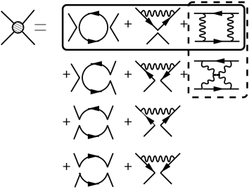
Figure 1: The NPRG $\beta$ function of the four-fermi operators. The diagrams in the solid box correspond to the ladder part, and the diagrams in the dashed box are crucial for the gauge independence. Possible other diagrams are ignored in our approximation.

Figure 2: The flow diagram in the $G_{2}-g$ plane in QCD. The phase structure does not appear, and all flows diverge at a certain finite scale.

There appears no phase boundary. All the flows diverge at a certain finite scale. Also we see the renormalized trajectory in the flow diagram which assures that the bare four-fermi interactions are irrelevant to the infrared physics. This behavior suggests that the entire region is supposed to be in the broken phase of the chiral symmetry. This is due to the infrared slavery behavior of the QCD gauge coupling constant and it is believed to hold naturally.

Renormalization group flows have been also analyzed  by the SD equation method[26], where fixing the quark mass obtained, the relation between the four-fermi coupling constant and the gauge coupling constant is calculated assuming the cutoff dependence of the gauge coupling constant. This procedure is justified within the SD formalism and it actually gave something resembling to the results in Fig. 2. However there are critical differences between these two calculations. The main difference comes from the fact that in the NPRG formalism the bare four-fermi interactions are turned out to be irrelevant, while in the SD formalism there is no mechanism to automatically generate effective four-fermi interactions by the gluon exchanges.

Correspondence between the divergence of the four-fermi operator and the dynamical chiral symmetry breaking is not trivial. All the coupling constants in the polynomial expansion keep growing in the infrared and diverge at some finite scale. This corresponds to the fact that at this scale the Wilsonian effective potential exhibits a non-analytical behavior at its origin, which is actually observed as a jump of the first derivative by direct analysis of the Wilsonian effective potential using the partial differential equation. This singularity at the origin clearly shows the spontaneous symmetry breakdown since it assures the non-vanishing magnetization at zero external field limit.

This singular behavior invalidates the renormalization group calculation of the evolution of the effective potential with polynomial expansion at the origin. Introducing a composite operator $\phi$ corresponding to the order parameter $\langle\bar{\psi}\psi\rangle$ enables us to carry out the calculation of the Wilsonian effective potential even in the infrared region.[21]  Our theory space is extended to include the composite operator $\phi$. First we introduce the composite operator $\phi$ as an auxiliary field in the original path integral without changing the dynamics. The partition function $Z$ in this extended theory space is written as

$$Z = \int{\cal D}\psi{\cal D}\bar{\psi}{\cal D}A\exp\left[\,-\int d^{4}x\ {\cal L}_{\rm org}\>[\psi,\bar{\psi},A\;]\;\right]$$ (13)

$$= \int{\cal D}\psi{\cal D}\bar{\psi}{\cal D}A{{\cal D}\phi}\exp\left[\,-\int d^{4}x\left\{{\cal L}_{\rm org}\>[\psi,\bar{\psi},A\;]+\frac{1}{2}(\phi-y\bar{\psi}\psi)^{2}\right\}\;\right].$$

Here we abbreviated the counter part $(\bar{\psi}i\gamma_{5}\psi)^{2}$ for simplicity and it should be considered that the original chiral symmetry is kept actually. Then the bare lagrangian is modified as follows:

$${\cal L} = {\cal L}_{\rm org}\>[\psi,\bar{\psi},A;\ t]+\frac{1}{2}(\phi-y\bar{\psi}\psi)^{2}$$ (14)

$$= \frac{1}{4}F^{a}_{\mu\nu}F^{a}_{\mu\nu}+\frac{1}{2\alpha}(\partial_{\mu}A_{\mu}^{a})^{2}+\bar{\psi}(\partial/-gA/-y\phi)\psi+\frac{1}{2}\phi^{2}+\frac{y^{2}}{2}(\bar{\psi}\psi)^{2}.$$

Even in case of omitting the chiral symmetric representation, this lagrangian has the discrete chiral symmetry:

$$\bar{\psi}\rightarrow\gamma_{5}\psi,\quad\psi\rightarrow-\bar{\psi}\gamma_{5},\quad\phi\rightarrow-\phi.$$ (15)

Then we may analyze the NPRG equations for the following Wilsonian effective potential:

$${\cal L}_{\scriptsize\rm eff} = \frac{1}{4}F^{a}_{\mu\nu}F^{a}_{\mu\nu}+\bar{\psi}(\partial/-gA/)\psi+V_{\scriptsize\rm eff}(\phi,\sigma;\ t),$$ (16)

$$V_{\scriptsize\rm eff}(\phi,\sigma;\ t) = \tilde{G}_{0}(\phi;\ t)+\sum^{nmax}_{n}\frac{1}{n}\tilde{G}_{n}(\phi;\ t)\ \sigma^{n}$$ (17)

$$= \tilde{G}_{0}(\phi;\ t)+\tilde{G}_{1}(\phi;\ t)\sigma+\frac{1}{2}\tilde{G}_{2}(\phi;\ t)\sigma^{2}+\cdots,$$

where the notation $\sigma=\bar{\psi}\psi$ is introduced. Note again that we are actually working with the chiral symmetric effective potential and we take a particular direction of the scalar operator $\sigma$ condensation to get the effective potential represented by Eq. (17). Since we do not consider the propagation of composite operator modes, Eq.(17) is enough to define the NPRG evolution of the chiral symmetric system.

In this formalism, it was shown that the chiral condensate $\langle\bar{\psi}\psi\rangle$ is proportional to the minimum position of the scalar potential $\tilde{G}_{0}(\phi)$, denoted by $\langle\phi\rangle$, which is the order parameter of the dynamical chiral symmetry breaking.

$$\langle\bar{\psi}\psi\rangle = \frac{1}{y}\langle\phi\rangle,$$ (18)

Then the dynamical mass of quarks $\Sigma(0)$ is given by

$$\Sigma(0) = \left.\frac{\partial V_{\scriptsize\rm eff}}{\partial\sigma}\right|_{\tiny\begin{array}[]{l}\phi=\langle\phi\rangle\\ \sigma=0\end{array}}=\tilde{G}_{1}(\phi=\langle\phi\rangle)$$ (21)

In the usual argument of introducing the auxiliary field, the four-fermi interaction is removed away from the action by tuning the Yukawa coupling constant $y$. Then this action may be regarded as the gauged Yukawa system with the compositeness condition.[6]  There are several studies of the dynamical chiral symmetry breaking by using this realization. However, we should notice that our purpose of introducing the auxiliary field $\phi$ is absolutely not to eliminate the four-fermi interaction. Also our results obtained by Eqs.(18) and (21) are turned out to be independent of the Yukawa coupling constant $y$,[21]  since it should not change the dynamics at all.

4 Compensation of the gauge dependence

As noted before, the ladder part NPRG exactly reproduces the results obtained by the ladder SD equations. Namely the results by the ladder part NPRG depend on the gauge parameter $\alpha$ strongly, like the ladder SD approaches. In order to improve the gauge dependence, we must proceed beyond the ladder approximation. So it is required to develop a non-ladder extended approximation in the course of the systematic approximation of NPRG.

To begin with, we discuss the origin of the gauge dependence in the ladder approximation. Let us consider a set of diagrams summed up by the ladder approximation. For that purpose we define the “massive” quark propagator,

$$\frac{1}{ip/-m(\phi,\sigma)},$$ (22)

where

$$m(\phi,\sigma) \equiv \frac{\partial V}{\partial\sigma}=\frac{\partial}{\partial\sigma}\sum_{n=1}^{nmax}\frac{\tilde{G}_{n}(\phi)}{n}\sigma^{n}=\sum_{n=1}^{nmax}\tilde{G}_{n}(\phi)\ \sigma^{n-1}$$ (23)

$$= \tilde{G}_{1}(\phi)+\tilde{G}_{2}(\phi)\sigma+\tilde{G}_{3}(\phi)\sigma^{2}+\tilde{G}_{4}(\phi)\sigma^{3}+\cdots.$$

Using the Feynman diagrams the “massive” quark propagator is represented as shown in Fig. 3.

Figure 3: The “massive” quark propagator. The deep full line in the left-handed side is a “massive” fermion propagator. The pale full lines are massless fermion operators and the dashed lines are the auxiliary fields $\phi$.

The ladder part $\beta$ functions are defined by summing up a set of diagrams which do not contain any crossed ladder type diagrams (Fig. 4).

$${\huge\frac{dV_{\scriptsize\rm eff}}{dt}=}$$

$+$

$+$

$+$

$+$

$+\cdots$

Figure 4: The ladder part $\beta$ function. These diagrams do not contain any crossed ladder type diagrams. The wavy lines are gluons, and the deep full lines are the “massive” quarks, and the pale full lines are external quark operators.

We now consider the Abelian Ward-Takahashi (WT) identities assuring the gauge independence. To satisfy WT identities we must sum over the diagrams for the S-matrix at any given order. When the gauge boson is inserted at a certain point along the fermion line, we must sum over all possible insertion points. Let us consider the simple case of WT identity involving two fermions and two gauge bosons in $g^{2}$ order.

+

Figure 5: The set of diagrams satisfying the Ward-Takahashi identity which involves two fermions and two gauge bosons. The wavy lines are gauge bosons and the full lines are fermions.

The sum of diagrams in Fig. 5 is gauge independent at on-shell. The right diagram of Fig. 5, called the crossed diagram, is not involved in the ladder approximation. This is one of the reason for the strong gauge dependence in the ladder approximation. Actually as seen in Fig. 2, adding the crossed box diagram to the $\beta$ function has wiped out the gauge dependence of the critical behaviors.[15]

Now we consider to generalize the crossed box diagrams in Fig. 2 for the $\beta$ functions of the higher multi-fermi operators. First we define a corrected vertex,

$$\frac{-2g^{2}}{p^{2}+m^{2}}\left[ip_{\alpha}\epsilon^{\mu\nu\alpha\beta}\gamma_{5}\gamma_{\beta}+mg^{\mu\nu}\right],$$ (24)

which is composed of “two” diagrams, ladder and crossed, using the “massive” quark propagator (Fig. 6). Therefore the corrected vertex itself comprises an infinite number of diagrams. Then we replace double vertices in Fig. 4 with the corrected vertex and sum up the diagrams just as the ladder part (Fig. 7).

= +

Figure 6: The corrected vertex. The wavy lines are gluons, and the deep full lines are “massive” quarks, and the pale full lines are external quark operators. The curved arrows denote the direction of the shell-mode momentum $p$.

$$\frac{dV}{dt}=\frac{d}{dt}\left\{\tilde{G}_{0}+\tilde{G}_{1}(\bar{\psi}\psi)+\frac{1}{2}\tilde{G}_{2}(\bar{\psi}\psi)^{2}+\frac{1}{3}\tilde{G}_{3}(\bar{\psi}\psi)^{3}+\frac{1}{4}\tilde{G}_{4}(\bar{\psi}\psi)^{4}+\cdots\right\}$$

$=$

$+$

$+~{}~{}\frac{1}{2}$

$+$

$+$

$+\cdots$

Figure 7: The $\beta$ function in our new approximation. The wavy lines are gluons, and the deep full lines are “massive” quarks, and the pale full lines are external quark operators.

Just as in Fig. 4, every diagram in Fig. 7 contributes to an infinite number of coupling constants in the polynomial expansion. Accordingly, a certain diagram with $n$ external quarks contributes to the $\beta$ functions of coupling constants with more than $n$ external quarks. For instance, the $\beta$ function of mass $\tilde{G}_{1}$ (the generalized Yukawa coupling) is given by the first and the second diagrams in Fig. 7. Also the $\beta$ function of the four-fermi operator comes from the first, the second and the third diagrams, etc. Note that the third diagram has a symmetry factor of 1/2.

Now we discuss the way of “projection” of the newly generated operators onto our target subspace. Here we consider the effective potential $V_{\scriptsize\rm eff}$ composed of the polynomials only in the scalar operator ${\cal O}_{1}$. Therefore we pick up only the parts proportional to $({\bf 1})^{n}$ in the spinor space from the generated total operators. For example, let us consider $g^{8}$ terms in the eight-fermi beta function (Fig. 8).

Figure 8: The newly generated $g^{8}$ operator. The numbers denote the suffixes of the quark fields (see Eq. (25)).

The form of the generated operators are in general,

$$\sum_{a,b,c,d}{\cal C}_{abcd}(\bar{\psi}_{1}\Gamma^{a}\psi_{1})\times(\bar{\psi}_{2}\Gamma^{b}\psi_{2})\times(\bar{\psi}_{3}\Gamma^{c}\psi_{3})\times(\bar{\psi}_{4}\Gamma^{d}\psi_{4}),$$ (25)

where $\Gamma$’s are the 16 independent matrices for spinor indices and ${\cal C}_{abcd}$ are amplitudes. We should consider all the parts proportional to $(\bar{\psi}{\bf 1}\psi)^{4}$ from the generated operators. Instead of picking up all of them, however, we take only one simple combination of $\Gamma$’s,

$$(\bar{\psi}_{1}{\bf 1}\psi_{1})\times(\bar{\psi}_{2}{\bf 1}\psi_{2})\times(\bar{\psi}_{3}{\bf 1}\psi_{3})\times(\bar{\psi}_{4}{\bf 1}\psi_{4}).$$ (26)

This part is represented in the left figure in Fig. 9. Of course there are another combinations of $\Gamma$’s contributing to $(\bar{\psi}{\bf 1}\psi)^{4}$ term, for example, contraction shown in the right figure in Fig. 9, which is omitted. We adopt this approximation since the left figure in Fig. 9 exactly coincides with the ladder part approximation, when the corrected vertices are replaced with the ladder type. We now challenge the minimal extension of the ladder approximation. We should mention that this restriction of the way of picking up $\sigma$ fields does not correspond to a general procedure of projection in the systematic approximation method of NPRG, and it might cause a problem.

Figure 9: The way of picking up $\sigma$. The left figure corresponds to the ladder part approximation, when the corrected vertices are replaced with the ladder type. We ignore the way of picking up $\sigma$ like the right figure.

Now let us consider the non-Abelian effects. The quarks belong to the 3 dimensional representation. For example, $g^{4}$ term in the four-fermi $\beta$ function from the ladder type diagram (Fig. 9) is identical to the Abelian estimate, except that we must add the color Casimir eigenvalue,

${\Rightarrow}~{}{\rm Tr}~{}(T^{a}T^{b}T^{b}T^{a})~{}=~{}3{C_{2}(3)^{2}}.$

Fig. 9. The gauge group factor of the box diagram in the four-fermi $\beta$ function.

As for the crossed ladder type diagrams (Fig. 4), there appears the commutator term $if^{abc}$ in addition to the Casimir term. Here we simply ignore the commutator term $if^{abc}$ and take account of the $C_{2}(3)^{2}$ term only.

${\Rightarrow}{\rm Tr}(T^{a}T^{b}T^{a}T^{b})=3C_{2}(3)^{2}+if^{abc}{\rm Tr}(T^{a}T^{b}T^{c}).$

Fig. 4. The gauge group factor of the crossed box diagram in the four-fermi $\beta$ function.

Of course this is a violent truncation which might break the gauge independence and it will be discussed later. Due to this additional approximation the non-Abelian nature is absorbed into the Casimir factor which defines the effective gauge coupling constant $C_{2}(3)g$. With this effective gauge coupling constant, the $\beta$ function of the effective potential in QCD is evaluated just as in the Abelian case.

Now we are able to write down general formulae of $g^{2n}$ terms in the NPRG equations as follows:

$$= -\frac{1}{8\pi^{2}}\frac{g^{2n}}{2^{n-2}\ n!}\ \frac{1}{(1+m^{2})^{n}}\ \frac{1}{1+\delta_{n,1}+\delta_{n,2}}$$ (27)

$$\times\left[m^{n}(3+{\alpha^{n}})+\sum_{k=1}^{[\frac{n}{2}]}(-)^{k}\frac{n!}{(2k)!\ (n-2k)!}(2+4^{k})m^{n-2k}\right]\sigma^{n}.$$

For example, the $\beta$ function for the four-fermi operator reads

$$\frac{d\tilde{G}_{2}}{dt} = -2\tilde{G}_{2}+\frac{1}{2\pi^{2}}\ \frac{\tilde{G}_{2}^{2}}{1+\tilde{G}_{1}^{2}}\left[1-\frac{2\tilde{G}_{1}^{2}}{1+\tilde{G}_{1}^{2}}\right]$$

$$+\frac{g^{2}}{4\pi^{2}}\ \frac{3+{\alpha}}{1+\tilde{G}_{1}^{2}}\left[\tilde{G}_{2}-\frac{2\tilde{G}_{1}^{2}\tilde{G}_{2}}{1+\tilde{G}_{1}^{2}}\right]+\frac{g^{4}}{16\pi^{2}}\ \frac{1}{\left[1+\tilde{G}_{1}^{2}\right]^{2}}\left[6-(3+{\alpha^{2}})\tilde{G}_{1}^{2}\ \right].$$

Let us compare above equation with the ladder approximated one,

$$\frac{d\tilde{G}_{2}}{dt} = -2\tilde{G}_{2}+\frac{1}{2\pi^{2}}\ \frac{\tilde{G}_{2}^{2}}{1+\tilde{G}_{1}^{2}}\left[1-\frac{2\tilde{G}_{1}^{2}}{1+\tilde{G}_{1}^{2}}\right]$$

$$+\frac{g^{2}}{4\pi^{2}}\ \frac{3+\alpha}{1+\tilde{G}_{1}^{2}}\ \left[\tilde{G}_{2}-\frac{2\tilde{G}_{1}^{2}\tilde{G}_{2}}{1+\tilde{G}_{1}^{2}}\right]+\frac{g^{4}}{32\pi^{2}}\frac{(3+\alpha)^{2}}{\left[1+\tilde{G}_{1}^{2}\right]^{2}}\ \left[1-\tilde{G}_{1}^{2}\right].$$

The gauge dependent terms in Eq. (4) should be almost compensated by the gauge dependent anomalous dimension of the quark fields when we go beyond the LPA, which will be discussed later.

5 Numerical Calculation and Results

Now we describe how to get the chiral order parameters in QCD with our approximation scheme. We work with the Wilsonian effective potential defined in Eq. (17) with some finite highest powers $nmax$, and we numerically integrate its NPRG equation. The NPRG equation is defined by the $\beta$ function given in Eq. (27), that is, we take only the quantum loops of the quarks and gluons and not of the scalar composites. The initial effective potential is taken from Eq. (14). During evolution the scalar field $\phi$ is fixed to be a certain value just as an external source field. The gauge coupling constant is set to follow the one-loop perturbative $\beta$ function with three flavor quarks. We take the QCD scale parameter $\Lambda_{\scriptsize\rm QCD}$ to be 490 MeV and we also adopt the same infrared cutoff scheme of the gauge coupling constant divergence as in Ref. [8], since our results should be first compared with the previous ladder SD results.[8]

Integrating the NPRG equation, the effective potential finally stops to move except for the canonical scaling behaviors, where the cutoff scale has been lowered well below the quark mass scale. Then we get the scalar potential $\tilde{G}_{0}(\phi)$ at the fixed $\phi$ value. To solve the NPRG equation scanning the fixed $\phi$ value, we obtain the scalar potential function $\tilde{G}_{0}(\phi)$ and its minimum point $\langle\phi\rangle$. Then we estimate the chiral condensates and the quark mass using Eqs. (18) and (21). The chiral condensates obtained above should be regarded as the bare operator condensation at the initial highest cutoff scale. It should be renormalized through the standard procedure to show the renormalized condensates at 1 GeV scale.

We show the results ($\alpha=0$ case) in Fig. 12. First of all we check the $nmax$ dependence of the results. Though there still remain some small fluctuations, we may claim that we have obtained the results of our total subspace of $nmax=\infty$. We have checked also that the dependence of the initial cutoff $\Lambda_{0}$ should be negligible, that is, our results are assured to be on the renormalized trajectory and we can regard them as those of the infinite initial cutoff limit.

Figure 12: The chiral condensates and the dynamical mass of quarks with their truncation dependence in the Landau gauge. The dashed line is $\Lambda_{\rm QCD}$. Non-ladder results are enhanced compared to the ladder results.

Now we compare our non-ladder extended results with the ladder ones. The ladder results exactly coincide with those of the ladder SD equation, which assures the total consistency of our calculational machinery. The chiral condensates and the quark mass are both enhanced by including the non-ladder contributions. Though we do not argue here in detail about the phenomenological implications of this enhancement, this enhancement is actually favorable for phenomenology since our setting of the QCD scale parameter has been recognized to be much higher than the current estimate even considering that it is the one-loop $\beta$ estimates.

The gauge parameter dependence of the results are depicted in Fig. 13. Compared with the ladder results, the improvement of gauge dependence of $\langle\bar{\psi}\psi\rangle$ is clearly seen in the left figure of Fig. 13. On the other hand the right figure of Fig. 13 shows that the gauge dependence of $\Sigma(0)$ still remains a lot even in the non-ladder approximation.

Figure 13: The gauge parameter dependence of the chiral condensates and the dynamical mass of quarks are plotted for cases $\alpha=0$ (Landau gauge), $\alpha=1$ (Feynman gauge) and $\alpha=2$.

We understand the different situations between these quantities as follows. The chiral condensate $\langle\bar{\psi}\psi\rangle$ is a measurable physical quantity. And it should not depend on the gauge. On the other hand the dynamical “mass” of quark $\Sigma(0)$ is an off-shell quantity and is not directly related to a measurable quantity; therefore, it may depend on the gauge. It should be noted also that the quark mass $\Sigma(0)$ strongly depends on the infrared cutoff scheme of the gauge coupling constant divergence while the chiral condensates do not.

6 Issues of the gauge dependence

In this section we discuss the origin of the gauge dependence in the NPRG method. First of all, the Wilsonian effective action $S_{\scriptsize\rm eff}$ itself depends on the gauge, because it is not directly related to any measurable quantities. Therefore the NPRG equations (or the $\beta$ function) describing the evolution of the Wilsonian effective action also depend on the gauge. Furthermore even at the infrared limit, the effective action is not totally gauge independent except for the on-shell quantities. For example the effective potential is not gauge independent except for the position of the minimum. Thus in general the $\beta$ function which depends on the gauge parameter finally gives the gauge independent results only for physical quantities at the infrared limit. Actually in our approximation scheme of evaluating the effective potential, there is no way of erasing all the gauge parameter dependence in the $\beta$ function.

We discuss here the gauge dependence due to the approximation we adopted, that is, the Local Potential Approximation. It ignores any corrections to the derivative couplings including the kinetic terms, and therefore no anomalous dimension is taken into account. This seems to be the largest source of the gauge dependence. We will report elsewhere the results taking account of the quark anomalous dimension, where we will see the reduced gauge dependence. Before getting these new results, we may evaluate the physical quantities as follows. In the one-loop approximation the quark anomalous dimension is proportional to $\alpha$, and therefore we have vanishing anomalous dimension in the Landau gauge $\alpha=0$. Therefore we may claim that the Landau gauge results in our scheme are most significant and they would be very near to the coming results with quark anomalous dimension. Then our main results should read,

$$\left.\frac{\langle\bar{\psi}\psi\rangle^{1/3}}{\Lambda_{\scriptsize\rm QCD}}\right|_{\rm\scriptsize non-ladder}=0.512\pm 0.014,$$ (30)

which is compared with the previous ladder results,

$$\left.\frac{\langle\bar{\psi}\psi\rangle^{1/3}}{\Lambda_{\scriptsize\rm QCD}}\right|_{\rm\scriptsize ladder}=0.439.$$ (31)

There are other subtleties of the gauge dependence due to the LPA. In the above calculation we have done further approximation to ignore some parts contributing to the $\beta$ functions. In Eq. (27) we omitted the non-Abelian commutator parts of the gauge effective vertex. This omission itself does not bring the gauge dependence. Rather it “hides” the gauge dependence of the LPA. Consider the four-fermi amplitude, for example. Such commutator parts should be summed up with diagrams in Fig. 14 (second derivative part of the gluon field, $\partial_{\mu}F_{\mu\nu}\bar{\psi}\gamma_{\nu}\psi$ as an operator form) to generate the gauge independent (on-shell) four-fermi amplitudes. This situation is quite the same as the Penguin diagram to give the local four-fermi effective operators.

Figure 14: The “Penguin”diagrams contributing to the four-fermi $\beta$ function.

Of course we also have to add all related diagrams in Fig. 15 and ghost diagrams to get totally gauge independent results with the properly renormalized gauge coupling constant.

Figure 15: The diagrams containing the wave function renormalization of the gauge field in the four-fermi amplitudes.

Therefore we have to take account of the derivative couplings $\partial_{\mu}F_{\mu\nu}\bar{\psi}\gamma_{\nu}\psi$ to compensate the gauge dependence appearing in the four-fermi box diagrams.

All these extension requires the higher order derivative couplings in our sub-theory space. Then we have to proceed to use smooth cutoff scheme NPRG equations since the sharp cutoff NPRG equations suffer singularities when applied to the derivative couplings.

7 Summary and Discussion

In this article we challenge a beyond the ladder calculation of the dynamical chiral symmetry breaking in QCD by using the non-ladder extension in the Non-Perturbative Renormalization Group method. The ladder approximation of the NPRG Local Potential $\beta$ function has been integrated to give exactly the same results of the (improved) ladder Schwinger-Dyson equation for the chiral condensates and the dynamical mass of quark $\Sigma(0)$. Extension beyond the ladder has strong motivation of reducing the inevitable gauge dependence of the ladder approximation.

We add non-ladder diagrams to the NPRG ladder $\beta$ function, trying to reduce the gauge dependence of the physical results. We develop a set of $\beta$ functions using the effective gluon vertex defined by the sum of the ladder and the crossed couplings. We numerically solve this new $\beta$ function to get the chiral condensates and quark mass function at zero momentum. They are enhanced compared with the previous ladder results, which are favorable phenomenologically. Also we evaluate the gauge parameter dependence of our results and find it is fairly reduced compared to the ladder case.

We stress here again that our results are the first results in the long history of analyzing the dynamical chiral symmetry breaking in gauge theories, which goes beyond the (improved) ladder equipping with a systematic approximation method. This is realized by quite a new viewpoint of the NPRG method for the dynamical chiral symmetry breaking.

References

- [1] Y. Nambu and G. Jona-Lasinio, Phys. Rev. 122 (1961), 345.
-
[2]
T. Maskawa and H. Nakajima, Prog. Theo. Phys. 52 (1974), 13261.
R. Fukuda and T. Kugo, Nucl. Phys. B117 (1976), 250.
V. V. Miransky, Nuovo Cim. 90A (1985), 149. -
[3]
K.-I. Kondo, H. Mino and K. Yamawaki, Phys. Rev. D39 (1989), 2430.
K. Yamawaki, in Proc. Johns Hopkins Workshop on Current Problems in Particle Theory 12, Baltimore, 1988, eds. G. Domokos and S. Kovesi-Domokos (World Scientific, Singapore, 1988).
T. Appelquist, M. Soldate, T. Takeuchi and L.C.R. Wijewardhana, ibid.
W. A. Bardeen, C. N. Leung and S. T. Love, Phys. Rev. Lett. 56 (1986), 1230.
C. N. Leung, S. T. Love and W. A. Bardeen, Nucl. Phys. B273 (1986), 649. -
[4]
K. Yamawaki, M. Bando and K. Matumoto, Phys. Rev. Lett.
56 (1986), 1335.
T. Akiba and T. Yanagida, Phys. Lett. B169 (1986), 432.
B. Holdom, Phys. Rev. D24 (1981), 1441. -
[5]
V. A. Miransky, M. Tanabashi and K. Yamawaki, Phys. Lett.
B221 (1989), 177.
B. Holdom, Phys. Rev. D54 (1996), 1068;
K. Yamawaki, hep-ph/9603293, in the proceedings of 14th Symposium on Theoretical Physics: Dynamical Symmetry Breaking and Effective Field Theory, Cheju, Korea, 21-26 Jul 1995. - [6] W. A. Bardeen, C. T. Hill and M. Lindner, Phys. Rev. D41 (1990), 1647.
- [7] K. Higashijima, Phys. Rev. D29 (1984), 1228.
-
[8]
K-I. Aoki, T. Kugo and M. G. Mitchard, Phys. Lett. B266 (1991),
467.
K-I. Aoki, M. Bando, T. Kugo, M. G. Mitchard and H. Nakatani, Prog. Theor. Phys. 84 (1990), 683. - [9] K-I. Aoki, M. Bando, T. Kugo, K. Hasebe and H. Nakatani, Prog. Theor. Phys. 81 (1989), 866.
-
[10]
K.-I. Kondo and H. Nakatani, Nucl. Phys. B351 (1991), 236;
Prog. Theor. Phys. 88 (1992), 7373.
K.-I. Kondo, Int. J. Mod. Phys. A7 (1992), 7239. - [11] K. G. Wilson and J. Kogut, Phys. Rep. 12 (1974), 75.
- [12] F.J.Wegner and A.Houghton, Phys. Rev. A8 (1973), 401.
-
[13]
J. Polchinski, Nucl. Phys. B231 (1984), 269.
G. Keller, C. Kopper and M. Salmhofer, Helv. Phys. Acta. 65 (1992),32. -
[14]
C. Wetterich, Phys. Lett. B301 (1993), 90.
M. Bonini, M. D’Attanasio and G. Marchesini, Nucl. Phys. B409 (1993), 441.
T. R. Morris, Int. J. Mod. Phys, A9 (1994), 2411. - [15] K-I. Aoki, K. Morikawa, J.-I. Sumi, H. Terao and M. Tomoyose, Prog. Theor. Phys. 97 (1997), 479.
- [16] K-I. Aoki, K. Morikawa, J.-I. Sumi, H. Terao and M. Tomoyose, Prog. Theor. Phys. 102 (1999), 1151.
-
[17]
K-I. Aoki, Prog. Theor. Phys. Suppl. 131 (1998), 129.
K-I. Aoki, to appear in Int. J. Mod. Phys. B.
T. R. Morris, Prog. Theor. Phys Suppl. 131 (1998), 395.
D. U. Jungnickel and C. Wetterich, Prog. Theor. Phys. Suppl. 131 (1998), 495 -
[18]
A. Hasenfratz and P. Hasenfratz, Nucl. Phys. B270 (1986), 269.
T. R. Morris, Phys. Lett, B334 (1994), 355. - [19] T. E. Clark, B. Haeri and S. T. Love, Nucl. Phys. B402 (1993), 628.
- [20] K-I. Aoki, K. Morikawa, W. Souma, J. I. Sumi and H. Terao, Prog. Theor. Phys. 95 (1996), 409; Prog. Theor. Phys. 99 (1998), 451.
- [21] K-I. Aoki, K. Morikawa, J.-I. Sumi, H. Terao and M. Tomoyose, hep-th/9908043, to appear in Phys. Rev. D61.
-
[22]
D. U. Jungnickel and C. Wetterich,
Lectures given at Workshop on the Exact Renormalization Group, Faro,
Portugal, 10-12 Sep 1998, hep-ph/9902316.
D. U. Jungnickel and C. Wetterich, Confinement, duality, and nonperturbative aspects of QCD (Cambridge 1997) 215-261.
J. Berges, D. U. Jungnickel and C. Wetterich, hep-ph/9811347.
H. Kouno, M. Nakai, A. Hasegawa and M. Nakano, nucl-th/9808058.
J. Berges, D. U. Jungnickel and C. Wetterich, Phys. Rev.D59 (1999), 34010.
M. Reuter and C. Wetterich, Phys. Rev. D56 (1997), 7893.
H. Kodama and J.-I. Sumi, hep-th/9912215, to appear in Prog. Theor. Phys.
K. Kubota and H. Terao, Prog. Theor. Phys. 102 (1999), 1163 - [23] C. Becchi, hep-th/9607181, On the construction of renormalized quantum field theory using renormalization group techniques, in Elementary Particles, Field Theory and Statistical Mechanics, ed. M. Bonini, G. Marchesini and E. Onofri (Parma University, 1993).
-
[24]
U. Ellwanger, Phys. Lett. B335 (1994), 364.
U. Ellwanger, M. Hirsch, and A. Weber, Z. Phys. C69 (1996), 687.
M. Bonini, M. D’Attanasio, and G. Marchesini, Nucl. Phys. B418 (1994), 81; B421 (1994), 429; B437 (1995), 163; Phys. Lett. B346 (1995), 87.
M. D’Attanasio, and T. R. Morris, Phys. Lett. B378 (1996), 213.
F. Freire, and C. Wetterich, Phys. Lett. B380 (1996), 337. - [25] T. R. Morris, hep-th/9810104, in Workwhop on the Exact Renormalization Group, to be published by World Scientific; hep-th/9910058.
- [26] K.-I. Kondo, S. Shuto and K. Yamawaki, Mod. Phys. Lett. A6 (1991), 3385.