Abstract

We argue that different aspects of Light-Front QCD at confined phase can be recovered by the Matrix Quantum Mechanics of D0-branes. The concerning Matrix Quantum Mechanics is obtained from dimensional reduction of pure Yang-Mills theory to 0+1 dimension. The aspects of QCD dynamics which are studied in correspondence with D0-branes are: 1) phenomenological inter-quark potentials, 2) whiteness of hadrons and 3) scattering amplitudes. In addition, some other issues such as the large-$N$ behaviour, the gravity–gauge theory relation and also a possible justification for involving “non-commutative coordinates” in a study of QCD bound-states are discussed.

PACS: 11.25.-w, 11.25.Sq, 12.38.-t, 12.38.Aw

Keywords: D-branes, QCD

1 Introduction

The idea of string theoretic description of gauge theories is an old one [1] [2]. Despite of the years passed on this idea, it is still activating different research works in theoretical physics [3][4][5][6]. On the other hand, in the last years our understanding about string theory is changed dramatically; a stream which is usually called the “second string revolution” [7]. The aim of this stream is formulating of a unified string theory as a fundamental theory of the known interactions. One of the most applicable tools in the above program are D$p$-branes [8, 9]. It is conjectured that D$p$-branes are perturbative representation of nonperturbative (strongly coupled) string theories.

It has been known for a long time that hadron-hadron scattering processes have two different behaviours depending on the amount of momentum transfer [10, 11]. At large momentum transfer interactions appear as interactions between the hadron constituents, partons or quarks, and some qualitative similarities to electron-hadron scattering emerge. At high energies and small momentum transfers Regge trajectories are exchanged. Regge trajectories provide a motivation for the first stringy picture of strong interaction. However, the good fitting between the Regge trajectories and the mass of strong bound-states is yet unexplained [1, 12] .

Deducing the apparently different observations above discussed from a unified picture is the challenge of theoretical physics and it is tempting to search for the application of the recent string theoretic progresses in this area. In this way one may find D$p$-branes good tools whose dynamics may be taken as a proper effective theory for the bound-states of quarks and QCD-strings (QCD electric fluxes). To use the string theory tools for QCD-strings one should replace the string theory parameters with those of QCD in a proper way. The case here is in the reverse direction of going from early days of string theory, as the theory of strong interaction, to string theory, as the theory of gravity.

To push the above idea, in two works [13, 14], taking the dynamics of D0-branes as a toy model, the potential and the scattering amplitude of two D0-branes were calculated. It is found that the potential between static D0-branes is a linear potential [15, 16, 17, 18]. Also the potential between two fast decaying D0-branes, which in the extreme limit see each other instantaneously, is calculated and the general results are found in agreement with phenomenology [15, 16, 18]. The scattering amplitude of two D0-branes was calculated in [14] based on the results of [19], it is shown that the cross section shows the Regge pole-expansion. Regge behaviour has been used some years ago to fit the hadron-hadron total cross section data successfully [20, 21] (see also [22, 23, 24, 25] for some more recent application of this behaviour).

Based on the results of [13][14] and some further discussions, we argue that different aspects of Light-Front formulation of QCD may be recovered by the Matrix Quantum Mechanics of D0-branes. In this paper we consider the Matrix Quantum Mechanics resulting from dimensional reduction of $d+1$ dimensional pure $U(N)$ YM theory to $0+1$ dimension. A detailed procedure of constructing this matrix mechanics is presented in [26]. In analogy with string theory ($d=9$ or 25), we call D0-branes the free-particles sector of the moduli space. We hope that these kinds of studies shed light on possible new relation between D-brane dynamics and gauge theories. Also we adjust our discussions to be in a reasonable contact with the known phenomenological aspects, though the exact match with experiments should not be expected at this level.

In Sec.2 we review the distinguished role of Light-Front coordinates for explaining the scaling behaviour of hadrons structure functions; the same behaviour which is taken as the consequence of point-like substructure in hadrons. In Sec.3 a short review of Matrix Quantum Mechanics of D0-branes is presented. In Sec.4 the calculation of the inter D0-branes potential will be presented. The discussion on the “whiteness” of D0-branes bound-states is given in Sec.5. In Sec.6 we deal with the problem of scattering. Sec.7 is devoted to discussions. Three issues are discussed in Sec.7: 1) large-$N$ limit, 2) quarks, gauge theory and gravity solutions relation and 3) non-commutativity. The discussion on the non-commutativity is on a possible justification for appearance “non-commutative” coordinates in the study of “non-Abelian” bound-states, such as bound-states of quarks and gluons.

2 QCD, Light-Cone And Constituent Quark Picture

Before gauge theoretic description of strong interaction, QCD, there was Constituent Quark Model (CQM) for hadrons. According to CQM a meson is just a quark-antiquark bound-state and a baryon is a three-quark one. The bound-state problem has been extensively studied for years by phenomenological inter-quark potentials to calculate various low-energy quantities. The agreement between calculated and observed quantities has been always too well to justify pursuing this approach to study hadron properties [15].

Presently QCD is established to be the underlying theory for strong bound-states and also it has been understood that QCD-vacuum is a very complicated medium. In low energy the coupling constant is large and so quantum fluctuations are highly excited. It means that basically “sea” of quarks and gluons have considerable contribution to the properties of hadrons. Moreover, the phenomena like confinement is believed to be direct consequences of the complex nature of the QCD-vacuum. So it seems that hadron picture of QCD is not reconcilable with any few-body picture of hadrons, like CQM (see [27] for a good discussion on this point).

Experimentally, substructure of hadrons is probed in sufficiently large momentum transfer scatterings of a fundamental particle, e.g. an electron, in the so-called Deep Inelastic Scattering (DIS) experiments. The existence of a point-like substructure, parton or quark, is taken as the reason for “scaling” behaviour of hadron structure-functions, i.e. the absence of any “scale” is the consequence of point-like objects [10]. Along the Bjorken’s argument, and as we recall it in below, this scaling behaviour has a simple interpretation in Light-Cone point of view on the processes which are involved in DIS. The story is the same for Feynman’s parton picture of DIS experiment and the Light-Cone Frame’s cousin, the Infinite Momentum Frame (IMF) [28]. By this simple interpretation of scaling in Light-Cone Frame we hopefully have a constituent picture for hadrons reconcilable with QCD, and it is the reason for developing the Light-Cone formulation of QCD during the past years [27, 29, 30].

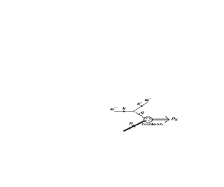
Figure 1: The lowest order process of DIS experiment.

The unpolarized cross-section of DIS in the lowest order is given by

$$k^{\prime}_{0}\frac{d\sigma}{d^{3}k^{\prime}}=\frac{2M}{s-M^{2}}\frac{\alpha^{2}}{Q^{4}}l_{\mu\nu}W^{\mu\nu},$$ (2.1)

with

$$W_{\mu\nu}(p,q) = \frac{1}{4M}\sum_{\sigma}\int\frac{d^{4}y}{2\pi}{\rm e}^{iq\cdot y}\langle p,\sigma|[J_{\mu}(y),J_{\nu}(0)]|p,\sigma\rangle,$$ (2.2)

$$l_{\mu\nu} = 2(k_{\mu}k^{\prime}_{\nu}+k_{\nu}k^{\prime}_{\mu}-\frac{1}{2}Q^{2}\eta_{\mu\nu}),\;\;q=k-k^{\prime},\;q^{2}=-Q^{2}<0.$$ (2.3)

$M$ and $s$ are the mass of the nucleon and total energy respectively. The momenta are specified in the Fig.1. Also, we define the useful parameters,

$$\nu=\frac{p\cdot q}{M},\;\;x=\frac{Q^{2}}{2M\nu},\;\;y=\frac{2M\nu}{s-M^{2}}.$$ (2.4)

Note that parameters $x$ and $y$ are dimensionless. In the rest frame of nucleon (target) we choose the z axis to be along the virtual photon momentum then we have

$$p=(M,0,0,0),\;\;\;\;\;q=(\nu,0,0,-\sqrt{\nu^{2}+Q^{2}}).$$ (2.5)

In the so-called Bjorken limit, $Q^{2}\rightarrow\infty$, $\nu\rightarrow\infty$ and $x$=fixed, we have $q=(\nu,0,0,-\nu-Mx)$. Now the statement of Bjorken scaling is as following: Up to a kinematical coefficient, the hadronic tensor $W_{\mu\nu}$ depends only on the parameter $x$ and not on $Q^{2}$. To see this, it is convenient to use Light-Cone variables $a^{\pm}=(a^{0}\pm a^{3})/\sqrt{2}$ with scalar product as $a\cdot b=a^{+}b^{-}+a^{-}b^{+}-a_{T}\cdot b_{T}$. Thus one writes

$$W_{\mu\nu}\sim\frac{1}{4M}\int dy^{-}{\rm e}^{iq^{+}y^{-}}\int dy^{+}d^{2}y_{T}{\rm e}^{iq^{-}y^{+}}\langle p|J_{\mu}(y)J_{\nu}(0)|p\rangle.$$ (2.6)

In the Bjorken limit we have

$$q^{+}\rightarrow-Mx/\sqrt{2}={\rm fixed},\;\;\;\;q^{-}=(2\nu+Mx)/\sqrt{2}\rightarrow\sqrt{2}\nu\rightarrow\infty.$$ (2.7)

In this limit the integrand of (2.6) contains the rapidly oscillating factor $\exp{(iq^{-}y^{+})}$ which kills all contributions to the integral except for those where the integrand is singular. Indeed the singularity of integrand comes from the current product at $y^{+}\sim 0$. In addition due to causality the integrand vanishes for $y^{2}=2y^{+}y^{-}-y_{T}^{2}<0$. So the dominant part of the integral comes from $y^{+}=y_{T}=0$. It explains the Bjorken scaling, i.e., the $q^{-}$ no longer exists at $y^{+}=0$. Now it is clear that the Light-Front coordinates play a distinguished role in the understanding of the scaling behaviour in DIS experiments. The same result is also correct for Feynman’s parton description of DIS and IMF, the experimental realization of Light-Cone Frame [28].

3 Matrix Quantum Mechanics Of D0-Branes

According to string theory, D$p$-branes are $p$ dimensional objects defined as (hyper)surfaces which can trap the ends of strings [9] and therefore it is reasonable to take their dynamics as a proper effective theory for the bound-states of quarks and QCD-strings (QCD electric fluxes).

One of the most interesting aspects of D-brane dynamics appears in their coincident limit. In the case of coinciding $N$ D$p$-branes their dynamics are captured by a $U(N)$ YM theory dimensionally reduced to $p+1$ dimensions of D$p$-brane world-volume [32, 9, 33]. In the case of D0-branes $p=0$, the above dynamics reduces to quantum mechanics of matrices, because time is the only parameter in the world-line. A detailed procedure of constructing this matrix mechanics is presented in [26]. The bosonic Lagrangian resulted from the pure YM is [34]

$$L=m_{0}{\rm Tr}\;\biggl{(}{\frac{1}{2}}D_{t}X_{i}^{2}+\frac{1}{4(2\pi\alpha^{\prime})^{2}}[X_{i},X_{j}]^{2}\biggl{)},$$

$$i,j=1,...,d,\;\;\;\;\;\;D_{t}=\partial_{t}-i[a_{0},\;],$$

where $\frac{1}{2\pi\alpha^{\prime}}$ and $m_{0}=(l_{s}g_{s})^{-1}$ are the string tension and the mass of D0-branes respectively ($l_{s}=\sqrt{\alpha^{\prime}}$ and $g_{s}$ are the string length and coupling, respectively). For $N$ D0-branes $X$’s are in adjoint representation of $U(N)$ and have the usual expansion $X_{i}=x_{i(a)}T_{(a)}$, $(a)=1,...,N^{2}$, .

The action (3) is invariant under the residual gauge symmetry of unreduced YM theory. The transformations are:

$$\vec{X} \rightarrow \vec{X^{\prime}}=U\vec{X}U^{\dagger},$$

$$a_{0} \rightarrow a^{\prime}_{0}=Ua_{0}U^{\dagger}+iU\partial_{t}U^{\dagger},$$ (3.2)

where $U$ is an arbitrary time-dependent $N\times N$ unitary matrix. Under these transformations one can check that:

$$D_{t}\vec{X} \rightarrow D^{\prime}_{t}\vec{X^{\prime}}=U(D_{t}\vec{X})U^{\dagger},$$

$$D_{t}D_{t}\vec{X} \rightarrow D^{\prime}_{t}D^{\prime}_{t}\vec{X^{\prime}}=U(D_{t}D_{t}\vec{X})U^{\dagger}.$$ (3.3)

First let us search for D0-branes in the above Lagrangian:
For each direction $i$ there are $N^{2}$ variables and not $N$ which one expects for $N$ particles. However there is an ansatz for the equations of motion which restricts the $U(N)$ basis to its $N$ dimensional Cartan subalgebra. This ansatz causes vanishing the potential and one finds the action of $N$ free particles, namely:

$$S=\int dt\sum_{(a)=1}^{N}{\frac{1}{2}}m_{0}\dot{\vec{x}}_{(a)}^{2}.$$ (3.4)

In this case the $U(N)$ symmetry is broken to $U(1)^{N}$ and the interpretation of $N$ remaining variables as the classical (relative) positions of $N$ particles is meaningful. The center of mass of D0-branes is represented by the trace of the $X$ matrices.

In the case of unbroken gauge symmetry the gauge transformations mix the entries of matrices and the interpretation of positions for D0-branes remains obscure [35]. Even in this case the center of mass is meaningful and the ambiguity about positions only remains for the relative positions of D0-branes. In unbroken phase the $N^{2}-N$ non-Cartan elements of matrices have a stringy interpretation; they govern the dynamics of low lying oscillations of strings stretched between D0-branes.

The dependences of energy eigenvalues and the size of bound-states are notable. By the scalings [34]

$$t \rightarrow g_{s}^{-1/3}t,$$

$$a_{0} \rightarrow g_{s}^{1/3}a_{0},$$

$$X \rightarrow g_{s}^{1/3}X,$$ (3.5)

one finds the relevant energy and size scales as

$$E \sim g_{s}^{1/3}/l_{s},$$

$$l_{d+2} = g_{s}^{1/3}l_{s}.$$ (3.6)

The length scale $l_{d+2}$ should be the fundamental length scale of the covariant $d+2$ dimensional theory whose Light-Cone formulation is argued to be described by action (3) with longitudinal momentum as $m_{0}$ [19]. So it is natural to assume in our case that $l_{d+2}$ (for $d=2$) is the inverse of the 3+1 dimensional QCD mass scale, denoted by $\Lambda_{QCD}$ . In the weak coupling $g_{s}\to 0$ ($m_{0}\gg l_{s}^{-1}$) one finds $l_{d+2}\ll l_{s}$ which allows to treat the bound-states of finite number of D0-branes as point-like objects in the transverse directions of the Light-Cone Frame , and consequently one finds $m_{0}\cdot E\sim\frac{1}{l_{d+2}^{2}}$, which shows the invariance under Lorentz transformation of this combination. As we will see in Sec.6 the masses of the intermediate states in the scattering amplitude appear as $l_{d+2}^{-1}$.

4 Known Potentials

To calculate the effective potential between D0-branes one should find the effective action around a classical configuration. This work can be done by integrating over the quantum fluctuations in a path integral. For the diagonal classical configurations, classical representations of D0-branes, the quantum fluctuations which must be integrated over are the off-diagonal entries. This work is equivalent to integrating over the oscillations of the strings stretched between D0-branes. Because here we deal with a gauge theory, and our interest is calculation around the classical field configuration, to obtain the effective action, it is convenient to use the background field method [37].

To calculate the effective action we write (3) in $d+1$ space-time dimensions in the form (in the units $2\pi\alpha^{\prime}=1$ and after the Wick rotation $t\rightarrow it$ and $a_{0}\rightarrow-ia_{0}$)

$$L = m_{0}{\rm Tr}\left(\frac{1}{4}[X_{\mu},X_{\nu}]^{2}\right),\;\;\;\mu,\nu=0,1,...,d,$$

$$X_{0} = i\partial_{t}+a_{0},\;\;\;\;S=\int Ldt,$$ (4.1)

where $\mu$ and $\nu$ are summed over by the Euclidean metric. The one-loop effective action of (4) has been calculated several times (e.g. see the Appendix of [38]) and the result can be expressed as

$$(\int dt)\;V(X_{\mu}^{cl})=\frac{1}{2}{\rm Tr}\log\bigg{(}P_{\lambda}^{2}\delta_{\mu\nu}-2iF_{\mu\nu}\bigg{)}-{\rm Tr}\log\bigg{(}P_{\lambda}^{2}\bigg{)},$$ (4.2)

with

$$P_{\mu}*\equiv[X_{\mu}^{cl},*],\;\;F_{\mu\nu}\;*\equiv[f_{\mu\nu},*],\;\;f_{\mu\nu}\equiv[X_{\mu}^{cl},X_{\nu}^{cl}],$$

and

$$P_{\lambda}^{2}=-\partial_{t}^{2}+\sum_{i=1}^{d}P_{i}^{2},$$ (4.3)

with the backgrounds $a_{0}^{cl}=0$. The second term in (4.2) is due to the ghosts associated with gauge symmetry.

4.1 Static Potential

Here we calculate the potential between two D0-branes at rest. The classical solution which represents two D0-branes in distance $r$ can be introduced as

$$X_{1}^{cl}={\frac{1}{2}}\left(\matrix{r&0\cr 0&-r}\right),\;\;X_{0}^{cl}=i\partial_{t}\left(\matrix{1&0\cr 0&1}\right),$$

$$a_{0}^{cl}=X_{i}^{cl}=0,\;\;\;i=2,...,d.$$ (4.4)

So one finds

$$P_{1}=\frac{r}{2}\otimes\Sigma_{3},\;\;P_{0}=i\partial_{t}\otimes 1_{4},\;\;P_{i}=0,\;\;\;i=2,...,d,$$ (4.5)

where $\Sigma_{3}$ is the adjoint representation of the third Pauli matrix , $\Sigma_{3}*=[\sigma_{3},*]$. The eigenvalues of $\Sigma_{3}$ are 0, 0, $\pm 2$.

The operator $P_{\lambda}^{2}$ is found to be

$$P_{\lambda}^{2}=-\partial_{t}^{2}\otimes 1_{4}+\frac{r^{2}}{4}\otimes\Sigma_{3}^{2},$$ (4.6)

which is a harmonic oscillator operator whose frequency, reintroducing $\alpha^{\prime}$, is $\omega\sim r/\alpha^{\prime}$. The one-loop effective action can be computed .

$$V(r) = (\frac{d-1}{2}){\rm Tr}\log\bigg{(}P_{\lambda}^{2}\bigg{)}$$ (4.7)

$$= -\;2(\frac{d-1}{2})\int_{0}^{\infty}\frac{ds}{s}\int_{-\infty}^{\infty}dk_{0}\;{\rm e}^{-s(k_{0}^{2}+r^{2})}$$

$$+\;{\rm traces\;independent\;of\;}r,$$

where 2 is for the degeneracy in eigenvalue 4 of $\Sigma_{3}^{2}$, and $k_{0}$ is for the eigenvalues of the operator $i\partial_{t}$. In writing the second line we have used

$$\ln\bigg{(}\frac{u}{v}\bigg{)}=\int_{0}^{\infty}\frac{ds}{s}\;({\rm e}^{-sv}-{\rm e}^{-su}).$$

The integrations can be performed and one finds

$$V(r) = -\;2(\frac{d-1}{2})\int_{0}^{\infty}\frac{ds}{s}(\frac{\pi}{s})^{{\frac{1}{2}}}{\rm e}^{-sr^{2}}$$ (4.8)

$$= \;4\pi(\frac{d-1}{2})\;|r|\;-\;\infty\;({\rm independent\;of\;}r).$$

The linear potential is the same of phenomenology interests, see e.g. [15, 17, 18]. Also it is the same which is consistent with spin-mass Regge trajectories [15, 16, 17, 18]. By restoring the $\alpha^{\prime}$ the potential will be found to be

$$V(r)=4\pi(\frac{d-1}{2})\frac{|r|}{2\pi\alpha^{\prime}}$$ (4.9)

which has the dimension $length^{-1}$. By comparison with Regge model one can have an estimation for $\alpha^{\prime}$ [16, 18]. The above potential can be used to describe an effective theory for the relative dynamics of D0-branes as

$$S=\int dt\bigg{(}\frac{1}{2}\frac{m_{0}}{2}\dot{\vec{r}}^{2}-4\pi(\frac{d-1}{2})\frac{|\vec{r}|}{2\pi\alpha^{\prime}}\bigg{)},$$ (4.10)

which in the range of validity of one-loop approximation, mentioned in previous footnote, it is expected to be applicable. Also by this action one obtains the energy scale as $E\sim\alpha^{\prime-2/3}m_{0}^{-1/3}\sim g_{s}^{1/3}/l_{s}$, as pointed in (3). The above action describes the dynamics in Light-Cone Frame with the longitudinal momentum $m_{0}$, and recalling (3) we have $p^{+}p^{-}\sim m_{0}E\sim g_{s}^{-2/3}l_{s}^{-2}\sim l_{d+2}^{-2}$.

It is not hard to see that the two D0-brane interaction potential is also true for every pair inside a bound-states of D0-branes. So the effective action for $N$ D0-branes is found to be

$$S=\int dt\bigg{(}\frac{1}{2}m_{0}\sum_{(a)=1}^{N}\dot{\vec{r}}_{(a)}^{2}-4\pi(\frac{d-1}{2})\sum_{(a)>(b)=1}^{N}\frac{|\vec{r}_{(a)}-\vec{r}_{(b)}|}{2\pi\alpha^{\prime}}\bigg{)}.$$ (4.11)

In a recent work [39], by taking the linear potential between quarks of a baryonic state in transverse directions of Light-Cone Frame, the structure functions are obtained with a good agreement with observed ones.

It is useful to relate the parameter $1/\alpha^{\prime}$ in the potential with gauge theory parameters. To do this we need a string theoretic description of gauge theory, but in the Light-Cone Frame. The nearest formulation we know for this is Light-Cone–lattice gauge theory (LClgt) [40]. In LClgt one assumes time direction and one of the spatial directions, say $z$, in continuum limit. The Light-Cone variables are defined as usual $x^{\pm}\sim t\pm z$. Other spatial directions naturally play the role of transverse directions of Light-Cone Frame, which are assumed to be on a lattice in LClgt. Due to existence of a continuous time $x^{+}$, there exists a Hamiltonian formulation [41] of the lattice gauge theory [42]. The relation between the linear confinement potential and gauge-lattice parameters is given by [41, 40]:

$$V(r)\sim\frac{g_{{}_{YM}}^{2}}{a^{2}}|r|,$$ (4.12)

with $a$ as the lattice spacing parameter in the transverse directions. Comparing this with (4.9) leads to

$$\frac{1}{\alpha^{\prime}}\sim\frac{g_{{}_{YM}}^{2}}{a^{2}}.$$ (4.13)

4.2 Fast Decaying D0-Branes

For two fast decaying D0-branes one can again calculate the above potential. This work can be done by inserting for example a Gaussian function for $k_{0}$ into the (4.7). This work is equivalent to restricting the eigenvalues of the operator $i\partial_{t}$. Having this in mind that eigenvalues of operators ($X,\;i\partial_{t}$, …) represent the information corresponding to classical values of D0-branes space-time positions , we find

$$V(r) = -2(\frac{d-1}{2})\int_{0}^{\infty}\frac{ds}{s}\int_{-\infty}^{\infty}dk_{0}\;\bigg{(}\frac{1}{\Delta}{\rm e}^{\frac{-k_{0}^{2}}{\Delta^{2}}}\bigg{)}{\rm e}^{-s(k_{0}^{2}+r^{2})}$$ (4.14)

$$= -2\sqrt{\pi}(\frac{d-1}{2})\int_{0}^{\infty}\frac{ds}{s}\frac{e^{-sr^{2}}}{\sqrt{s\Delta^{2}+1}},$$ (4.15)

in which we assumed that the D0-branes live around time zero. The last expression is infinite, but one can show that the infinite part is $r$-independent. One takes:

$$\frac{\partial V(r)}{\partial(r^{2})}=2\sqrt{\pi}(\frac{d-1}{2})\int_{0}^{\infty}\frac{dse^{-sr^{2}}}{\sqrt{s\Delta^{2}+1}},$$ (4.16)

which is finite and so infinity of $V(r)$ is $r$-independent. The last integral can not be calculated exactly, though numerical comparison with phenomenology is possible. The limit $\Delta\rightarrow 0$ can be calculated exactly by recalling the relation:

$$\lim_{\Delta\rightarrow 0}\bigg{(}\frac{1}{\Delta}e^{-\frac{k_{0}^{2}}{\Delta^{2}}}\bigg{)}=\sqrt{\pi}\delta(k_{0}).$$

Inserting $\delta$-function in (4.14) one finds:

$$V(r)\sim-2(\frac{d-1}{2})\int_{0}^{\infty}\frac{ds}{s}\;{\rm e}^{-s(r^{2})}\;\sim\;\ln r,$$ (4.17)

which the last result is after extracting the $r$-independent infinity. This result is already consistent with phenomenology of heavy quarks [18, 16], which we know their weak decay rates grow with $(mass)^{5}$. In the extreme limit $\Delta\rightarrow 0$, in which the two D0-branes see each other “instantaneously”, one can take them as two D(-1)-branes (D-instantons). The dynamics of D(-1)-branes are described by the action (4) but instead of the taking $X_{0}$ as $i\partial_{t}$ one takes $X_{0}$ as a matrix which its eigenvalues represent the “instants” which D(-1)-branes occur. So the above logarithmic result also could be obtained in D(-1)-branes calculation by taking a classical solution as

$$X_{1}^{cl}={\frac{1}{2}}\left(\matrix{r&0\cr 0&-r}\right),\;X_{0}^{cl}=\left(\matrix{t_{0}&0\cr 0&t_{0}}\right),\;\;a_{0}^{cl}=X_{i}^{cl}=0,\;\;i=2,...,d,$$ (4.18)

which represents two D(-1)-branes appeared at time $t_{0}$, in distance $r$.

A comment is in order: from phenomenological point of view, it is known that in some cases potentials like $r^{\xi}$, with $\xi\simeq 0.1$ also have produced good results [18, 16]. This maybe can be included to our intermediate result (4.14) or logarithmic result by recalling the numerical relation $\ln r\simeq r^{\eta\simeq 0}$, which is valid for a range of $r$ .

5 White States

To determine the color of an object its dynamics should be studied in presence of external fields. For a “white” extended object, the center of mass (c.m.) moves as a free particle in a uniform electric field. Now we want to specify the color of the D0-branes bound-states. As we will see, although our formulation for dynamics of D0-branes in external YM fields seems incomplete, but there is a reasonable statement about “whiteness” of D0-branes bound-states.

5.1 D0-Branes In YM Background

In classical Electrodynamics besides electromagnetic fields produced by different distributions of charges and currents, we also study the dynamics of a charged particle in regions of space where electromagnetic fields exist. There is a simple question: What are the problems arising when one studies Chromodynamics in this level?

The main problem arises when one introduces sources and matches Chromodynamics with dynamics of colored objects (for example a colored particle). In case of Electrodynamics there is a simple relation. For example the equation of motion of a charge particle with mass $m_{0}$ and charge $q$ is

$$m_{0}\ddot{\vec{x}}=q(\vec{E}+\vec{v}\times\vec{B}).$$ (5.1)

The concept of gauge invariance at this level is understood as the invariance of equations of motion under gauge transformations, i.e. field strengths are invariant under gauge transformations. Now, in the case of Chromodynamics right-hand-side is a matrix and transforms as an object in adjoint representation under gauge group transformations, as

$$\vec{E}\rightarrow\vec{E}^{\prime}=U\vec{E}U^{\dagger},\;\;\;\;\vec{B}\rightarrow\vec{B}^{\prime}=U\vec{B}U^{\dagger}.$$ (5.2)

So the problem arises. As it is well-known for string theorists, now we have a good candidate for non-commutative coordinates which are the coordinates of coincident D0-branes. First one may rewrite (5.1) for “matrix” coordinates as

$$m_{0}{\ddot{\vec{X}}}=q(\vec{E}+{\dot{\vec{X}}}\times\vec{B}),$$ (5.3)

but it is not enough to have correct behaviour for the first side under gauge transformations. Here the world-line gauge symmetry (3) of D0-brane dynamics helps us, to write the generalized Lorentz equation as ,

$$m_{0}D_{t}D_{t}\vec{X}=q(\vec{E}+D_{t}\vec{X}\times\vec{B}).$$ (5.4)

By recalling the relation (3) one observes that both sides have the same behaviour under gauge transformations. However, it seems that the picture is not complete yet. First, it is not clear what is the Lagrangian formulation of this problem. Secondly, the precise meaning of position dependences of field strengths should be clarified (there is the same question for $U$, the parameter of gauge transformation).

Now, the crucial observation is the decoupling of c.m. dynamics from non-Abelian parts. It is because of trace nature of $U(1)$ and $SU(N)$ parts. As we mentioned earlier the c.m. degree of freedom is described by the $U(1)$ part of $U(N)$ [32]. So the position and the momentum of c.m. can be obtained by a simple trace [35]

$$\vec{x}_{c.m.}\equiv\frac{1}{N}\;{\rm Tr}\vec{X},\;\;\;\;\;\vec{p}_{c.m.}\equiv\;{\rm Tr}\vec{P}.$$ (5.5)

To investigate the kind and amount of the charge of an object its dynamics should be studied in absence of magnetic field ($\vec{B}=0$) and (for extended objects) in uniform electric field ($\vec{E}(x)=\vec{E}_{0}$). So the c.m. equation of motion is

$$m_{0}\ddot{\vec{x}}_{c.m.}=q\vec{E}_{(1)0},$$ (5.6)

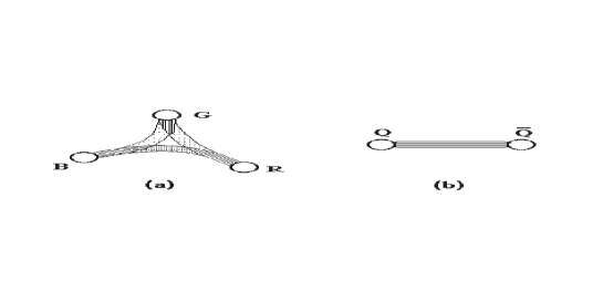
Figure 2: The net electric flux extracted from each quark is equivalent in a baryon (a) and a meson (b). The D0-brane–quark correspondence suggests the string-like shape for fluxes inside a baryon (a).

which the subscript (1) denotes that the corresponding electric field comes from the $U(1)$ part of $U(N)$. It is understood that the dynamics of c.m. will not be affected by the non-Abelian part of gauge group. It means that the c.m. is white with respect to $SU(N)$. This behaviour of D0-branes bound-states is the same as that of hadrons. It means that each D0-brane feels the net effect of other D0-branes as the white-complement of its color. In other words, the field fluxes extracted from one D0-brane to the other ones are the same as the flux between a color and an anti-color, Fig.2. As we have shown in Sec.4, there is a linear potential between each two static D0-branes, which is consistent with this flux-string picture. Also, the number of D0-branes in the bound-state, $N$, equals to that of baryons. As we mentioned before, recently [39] the linear potential between the constituents of baryons, in the transverse directions of Light-Cone Frame, has been used successfully to obtain the structure functions.

As the final note in this part, we remind that the dynamics presented by (5.1) can be taken as for a massless particle in transverse directions in Light-Cone Frame with longitudinal momentum, $p^{+}\equiv m_{0}$. The fields $\vec{E}$ and $\vec{B}$ are electromagnetic fields in transverse directions. We present the derivation of this in the Appendix.

6 Scattering Amplitude

As a consequence of asymptotic freedom, in a suddenly collision process quarks or partons are assumed to be free. So the probe, an electron or another quark, only interacts with the hadron constituents instead of the hadron as a whole [10, 11]. It is the same mechanism which results scaling behaviour in hadron structure functions.

With the above in mind it is reasonable to calculate the scattering amplitude between two individual D0-branes, to find an impression about the behaviour of the scattering amplitude of two hadrons which D0-branes are assumed as their quarks. Also it is natural to assume that this result is for high energy-elastic regime of hadron collisions.

Here we use the result of [19]. In [19] it is shown that the quantum travelling of D0-branes can be understood by the field theory Feynman graphs and corresponding amplitudes in the Light-Cone Frame. In the following we review the approach to calculate the amplitude.

We concentrate on the limit $\alpha^{\prime}\rightarrow 0$. In this limit to have a finite energy one has

$$[X_{i},X_{j}]=0,\;\;\;\forall\;i,j,$$ (6.1)

and consequently the potential term in the action vanishes. So, D0-branes do not interact and the “classical action” reduces to the action of $N$ free particles. We take this classical action also in the quantum case too, it is equivalent to the assumption that two quarks in two spatially well separated hadrons do not interact with each other. Since hadrons are white one can trust this assumption. However, the above observation fails when D0-branes arrive each other. When two D0-branes come very near each other two eigenvalues of $X_{i}$ matrices will be equal and the corresponding off-diagonal elements can get non-zero values. This is the same story of gauge symmetry enhancement. The fluctuations of these off-diagonal elements are responsible for the interaction between D0-branes in bound-states.

In the coincident limit the dynamics is complicated. The relative matrix position may be taken as:

$$\vec{X}=\left(\matrix{\vec{r}/2&\vec{Y}\cr\vec{Y}^{*}&-\vec{r}/2}\right),$$ (6.2)

where $Y^{*}$ is the complex conjugate of $Y$. By inserting this matrix into the Lagrangian one obtains:

$$S = \int dt{\frac{1}{2}}\bigg{(}(2m_{0})\dot{\vec{X}}_{c.m.}^{2}+m_{0}\dot{\vec{Y}}\cdot\dot{\vec{Y}}^{*}-\frac{m_{0}}{4}\frac{1}{4(2\pi\alpha^{\prime})^{2}}(1-\cos^{2}\theta)\vec{r}^{{}^{2}}\vec{Y}\cdot\vec{Y}^{*}$$ (6.3)

$$+ \frac{m_{0}}{2}\dot{\vec{r}}^{2}+O(Y^{3})\bigg{)},$$

with $X_{c.m.}$ for the center of mass and $\theta$ is the angle between $\vec{r}$ and the complex vector $\vec{Y}$. As it is apparent in the $\alpha^{\prime}\rightarrow 0$ limit which is the case of our interest, the $r$ element do not take large values and have a small range of variation. In high-tension approximation of strings ($\alpha^{\prime}\rightarrow 0$), one can take the separation of D0-branes a constant of order $r\sim g_{s}^{1/3}l_{s}$. As is noted in Sec.3, this length is the typical size of the D0-brane bound-states. So,

$$S=\int dt\bigg{(}{\frac{1}{2}}(2m_{0})\dot{\vec{X}}_{c.m.}^{2}+{\frac{1}{2}}m_{0}\dot{Y}_{\perp}\cdot\dot{Y}_{\perp}^{*}-{\frac{1}{2}}m_{0}\frac{k^{2}r^{2}}{\alpha^{\prime 2}}Y_{\perp}\cdot Y_{\perp}^{*}+{\frac{1}{2}}\frac{m_{0}}{2}\dot{\vec{r}}+\cdot\cdot\cdot\bigg{)},$$ (6.4)

where in the above $k$ is a numerical factor depending on $\alpha^{\prime}$ and $g_{s}$ , and $Y_{\perp}$ is the part of the $\vec{Y}$ perpendicular to the relative distance $\vec{r}$. The parallel part of $\vec{Y}$ behaves as a free part. In $d+1$ dimensions of space-time the dimension of $Y_{\perp}$ is $d-1$ which shows that we are encountered with $2\times(d-1)$ harmonic oscillators because, $Y$ is a complex variable. This is the same number of harmonic oscillators which appears in one-loop calculations (Sec.4). These harmonic oscillators correspond to vibrations of (oriented) open strings stretched between D0-branes. In the following we ignore the radial momentum and even the angular momentum by dropping the term $m_{0}\dot{\vec{r}}^{2}$ and set $r=r_{0}$ for simplicity .

For two D0-branes we take the probability amplitude presented by path integral as

$$\langle x_{3},x_{4};t_{f}|x_{1},x_{2};t_{i}\rangle=\int{\rm e}^{-S}.$$ (6.5)

Based on the previous discussion, in the $\alpha^{\prime}\rightarrow 0$ limit for (Fig.3) graph we decompose the path-integral as the following, ,

$$\langle x_{3},x_{4};t_{f}|x_{1},x_{2};t_{i}\rangle=\left[\int{\rm e}^{-S}\right]_{\alpha^{\prime}\rightarrow 0}=\int_{t_{i}}^{t_{f}}dT_{1}dT_{2}\int_{-\infty}^{\infty}dX_{1}dX_{2}$$ (6.6)

$$\times\bigg{(}K_{m_{0}}(X_{1},T_{1};x_{1},t_{i})K_{m_{0}}(X_{1},T_{1};x_{2},t_{i})\bigg{)}$$

$$\times\bigg{(}K_{2m_{0}}(X_{2},T_{2};X_{1},T_{1})K_{oscillator}(Y_{\perp}=0,T_{2};Y_{\perp}=0,T_{1})\bigg{)}$$

$$\times\bigg{(}K_{m_{0}}(x_{3},t_{f};X_{2},T_{2})K_{m_{0}}(x_{4},t_{f};X_{2},T_{2})\bigg{)},$$

which $K_{m}(y_{2},t_{2};y_{1},t_{1})$ is the non-relativistic propagator of a free particle with mass $m$ between $(y_{1},t_{1})$ and $(y_{2},t_{2})$ and $K_{oscilator}(Y_{\perp}=0,T_{2};Y_{\perp}=0,T_{1})$ is the harmonic oscillator propagator. $\int dT_{1}dT_{2}dX_{1}dX_{2}$ is for a summation over different “Joining-Splitting” times and points. We use in $d$ dimensions the representations

$$K_{m}(y_{2},t_{2};y_{1},t_{1})=\theta(t_{2}-t_{1})\frac{1}{(2\pi)^{d}}\int d^{d}p\;{\rm e}^{ip\cdot(y_{2}-y_{1})-\frac{ip^{2}(t_{2}-t_{1})}{2m}},$$

$$K_{oscilator}(Y_{\perp}=0,T_{2};Y_{\perp}=0,T_{1})=\theta(T_{2}-T_{1})\bigg{(}\frac{m_{0}\omega}{2\pi i\sin[\omega(T_{2}-T_{1})]}\bigg{)}^{d-1},$$

where $\theta(t_{2}-t_{1})$ is the step function and $\omega$ is the harmonic oscillator frequency, $\omega\sim kr_{0}/\alpha^{\prime}\sim kg_{s}^{1/3}/l_{s}$. Because of complex nature of $Y_{\perp}$ the power for the harmonic propagator is $2\times\frac{d-1}{2}$.

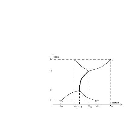
Figure 3: A typical tree path of D0-branes.

All the above results can be translated into the momentum space ($E_{k}=\frac{p_{k}^{2}}{2m_{0}}$ with $k=1,2,3,4$):

$$\langle p_{3},p_{4};t_{f}|p_{1},p_{2};t_{i}\rangle \sim {\rm e}^{i(E_{3}+E_{4})t_{f}-i(E_{1}+E_{2})t_{i}}\int\prod_{a=1}^{4}dx_{a}{\rm e}^{i(p_{1}x_{1}+p_{2}x_{2}-p_{3}x_{3}-p_{4}x_{4})}$$ (6.7)

$$\times\langle x_{3},x_{4};t_{f}|x_{1},x_{2};t_{i}\rangle.$$

This representation is useful to calculate the cross section. The integrals can be performed and we find

$$\langle p_{3},p_{4};t_{f}|p_{1},p_{2};t_{i}\rangle\sim\delta^{(d)}(p_{1}+p_{2}-p_{3}-p_{4})\int_{t_{i}}^{t_{f}}dT_{1}dT_{2}\theta(T_{2}-T_{1})$$ (6.8)

$$\times\exp(\frac{-i(p_{1}^{2}+p_{2}^{2})T_{1}}{2m_{0}})\exp(\frac{-iq^{2}(T_{2}-T_{1})}{4m_{0}})\exp(\frac{i(p_{3}^{2}+p_{4}^{2})T_{2}}{2m_{0}})$$

$$K_{oscillator}(Y_{\perp}=0,T_{2};Y_{\perp}=0,T_{1})$$

where $\vec{q}=\vec{p}_{1}+\vec{p}_{2}=\vec{p}_{3}+\vec{p}_{4}$.

To have a real scattering process let us assume

$$t_{i}\rightarrow-\infty,\;\;\;t_{f}\rightarrow\infty.$$

We put $T\equiv T_{2}-T_{1}$ which has the range $0\leq T\leq\infty$. The integrals yield

$$\langle p_{3},p_{4};\infty|p_{1},p_{2};-\infty\rangle \sim \delta^{(d)}(p_{1}+p_{2}-p_{3}-p_{4})\delta(\frac{p_{1}^{2}}{2m_{0}}+\frac{p_{2}^{2}}{2m_{0}}-\frac{p_{3}^{2}}{2m_{0}}-\frac{p_{4}^{2}}{2m_{0}})$$ (6.9)

$$\int_{0}^{\infty}dT\;{\rm e}^{\frac{-iT}{4m_{0}}(q^{2}-2(p_{1}^{2}+p_{2}^{2}))}\bigg{(}\frac{m_{0}\omega}{\sin(\omega T)}\bigg{)}^{d-1}.$$

Recalling the energy-momentum relation in the Light-Cone gauge [19],

$$2(p_{1}^{2}+p_{2}^{2})-\vec{q}^{\;2}=2(2m_{0})(\frac{p_{1}^{2}+p_{2}^{2}}{2m_{0}})-\vec{q}^{\;2}=2q^{+}q^{-}-\vec{q}^{\;2}=q_{\mu}q^{\mu}\equiv q_{\mu}^{2},$$

we find

$$\langle p_{3},p_{4},E_{3},E_{4};\infty|p_{1},p_{2},E_{1},E_{2};-\infty\rangle \sim \delta^{(d)}(p_{1}+p_{2}-p_{3}-p_{4})\delta(E_{1}+E_{2}-E_{3}-E_{4})$$ (6.10)

$$\int_{0}^{\infty}dT{\rm e}^{\frac{-q_{\mu}^{2}}{4m_{0}}T}\bigg{(}\frac{m_{0}\omega}{\sin(\omega T)}\bigg{)}^{d-1}.$$

We perform a cut-off for $T$ in small values as $0<\epsilon\leq T\leq\infty$, with $\epsilon$ be small . By changing the integral variables as ${\rm e}^{-2\omega T}=\eta$, we have

$$\langle p_{3}^{\mu},p_{4}^{\mu};\infty|p_{1}^{\mu},p_{2}^{\mu};-\infty\rangle \sim \delta^{(d)}(p_{1}+p_{2}-p_{3}-p_{4})\delta(p_{1}^{-}+p_{2}^{-}-p_{3}^{-}-p_{4}^{-})$$ (6.11)

$$\frac{(m_{0}\omega)^{d-1}}{2\omega}\int_{0}^{x}d\eta\;\eta^{\frac{-q_{\mu}^{2}}{8m_{0}\omega}+\frac{d-3}{2}}(1-\eta)^{-d+1},$$

$$\sim \delta^{(d)}(p_{1}+p_{2}-p_{3}-p_{4})\delta(p_{1}^{-}+p_{2}^{-}-p_{3}^{-}-p_{4}^{-})$$

$$\frac{(m_{0}\omega)^{d-1}}{2\omega}B_{x}(\frac{-q_{\mu}^{2}}{8m_{0}\omega}+\frac{d-1}{2},-d+2)$$

where $1\sim x={\rm e}^{-2\omega\epsilon}$ and $B_{x}$ is the Incomplete Beta function. The longitudinal momentum conservation trivially is satisfied. Furthermore, because of the conservation of this momentum we do not expect so-called $t$-channel processes here.

6.1 Polology

Equivalently one may use the other representation of $K_{oscillator}$ as

$$K_{oscillator}(Y_{\perp}=0,T_{2};Y_{\perp}=0,T_{1})=\sum_{n}\langle 0|n\rangle\langle n|0\rangle{\rm e}^{-iE_{n}(T_{2}-T_{1})},$$ (6.12)

with $E_{n}$’s as the known $H_{oscillator}$ eigenvalues. In this representation one finds the pole expansion [19]:

$$\langle p_{3}^{\mu},p_{4}^{\mu};\infty|p_{1}^{\mu},p_{2}^{\mu};-\infty\rangle \sim \delta^{(d)}(p_{1}+p_{2}-p_{3}-p_{4})\delta(p_{1}^{-}+p_{2}^{-}-p_{3}^{-}-p_{4}^{-})$$ (6.13)

$$\times\lim_{\epsilon\rightarrow 0^{+}}\sum_{n}C_{n}\;\frac{i4m_{0}}{q_{\mu}q^{\mu}-M_{n}^{2}+i\epsilon}.$$

This pole expansion also can be derived by extracting the poles of the amplitude (6.11) with the condition

$$\frac{-q_{\mu}^{2}}{8m_{0}\omega}+\frac{d-1}{2}=-n,\;\;{\rm with}\;n\;{\rm as\;a\;positive\;integer}.$$ (6.14)

Hence for the mass of the intermediate bound-states we obtain

$$M_{n}^{2}=\frac{8k(n+\frac{d-1}{2})}{(g_{s}^{1/3}l_{s})^{2}}.$$ (6.15)

We recall that the combination $g_{s}^{1/3}l_{s}$ is $l_{d+2}$, the fundamental length of $d+2$ dimensional theory (Sec.3 and [19]). The Regge pole-expansion of (6.11)-(6.15) is the phenomenological promising feature of this amplitude [20, 21, 22, 23, 24, 25].

7 Discussion

In this section we discuss some relevant issues: 1) large-$N$ limit, 2) quark, gauge theory and gravity solutions relations and also 3) non-commutativity.

7.1 Large-$N$

Baryons show special properties in large-$N$ limit of gauge theories [43]

• Their mass grows linearly by $N$.

• Their size do not depend on $N$. So their density goes to infinity at large-$N$.

• Baryon-baryon force grows proportionally with $N$.

These properties mainly are extracted from a Hamiltonian formulation for baryons as a bound-state of $N$ quarks. Based on an approximation to approach the $N$-body problem (Hartree approximation), the above properties can be justified for baryons at large-$N$.

Here we try to work out the Hamiltonian formulation, and then the above mentioned properties are followed by the same reasoning of [43] .

In Sec.4 the effective theory for D0-branes were obtained to be

$$S=\int dt\bigg{(}\frac{1}{2}m_{0}\sum_{(a)=1}^{N}\dot{\vec{r}}_{(a)}^{2}-4\pi(\frac{d-1}{2})\sum_{(a)>(b)=1}^{N}\frac{|\vec{r}_{(a)}-\vec{r}_{(b)}|}{2\pi\alpha^{\prime}}\bigg{)}.$$ (7.1)

Also we have found the relation between the $\alpha^{\prime}$ parameter and the coupling constant of gauge theory by comparing it to LClgt, namely $\frac{1}{\alpha^{\prime}}\sim\frac{g_{{}_{YM}}^{2}}{a^{2}}$ where $a$ is the lattice spacing parameter. It is known that it is more convenient to replace the coupling constant by $\frac{g_{{}_{YM}}}{\sqrt{N}}$ at large-$N$ [43]. So the action in terms of new parameters is

$$S=\int dt\bigg{(}\frac{1}{2}m_{0}\sum_{(a)=1}^{N}\dot{\vec{r}}_{(a)}^{2}-4\pi(\frac{d-1}{2})\frac{g_{{}_{YM}}^{2}}{a^{2}}\frac{1}{N}\sum_{(a),(b)=1}^{N}|\vec{r}_{(a)}-\vec{r}_{(b)}|\bigg{)},$$ (7.2)

and the associated Hamiltonian is the same used in [43] except for the potential term, which is Coulomb one there.

Here we just check the mass of baryons at large-$N$. The kinetic term of c.m., $\frac{\vec{P}^{2}}{Nm_{0}}$, grows with $N$, and the net potential for each D0-brane takes a factor $\frac{1}{2}N(N-1)$ due to pair interactions. So the potential term at large-$N$ grows like

$$\frac{1}{2}N(N-1)\frac{g_{{}_{YM}}^{2}}{N}\sim N.$$ (7.3)

It results that the energy grows as $E\sim N$ at large-$N$. From the point of view of Light-Cone Frame the energy is $P^{-}$. The total longitudinal momentum of this bound-state is $P^{+}=Np^{+}$, where $p^{+}=m_{0}$ is the longitudinal momentum of one D0-brane. Consequently, the invariant mass $M$ is

$$M^{2}=2P^{+}P^{-}-\vec{P}^{2}\sim N^{2}\Rightarrow M\sim N.$$ (7.4)

7.2 Quarks, Gauge Theory And Schwartzschild Solutions Of Gravity

D$p$-branes are $p$ dimensional Schwartzschild solutions of low energy effective field theories of string theories . So any proposal for equivalence between them and quarks, or at least between their dynamics and quarks dynamics, may need justification at first. Here we recall some string theoretic related issues shortly, and also try to present (maybe) a non-string theoretic related feature then.

As mentioned, D-branes are gravity solutions. On the other hand, it is known that the dynamics of these objects are captured by a gauge theory. It is one of the closest connections between gauge theories and gravity, which has been revealed by string theory. Through this relation between the dynamics of an extended object and a gauge theory, many studies have been done to develop understanding of gauge theory dynamics. One of the recent progresses in this area is the adS/CFT correspondence [6], to relate gauge theory dynamics at large ’t Hooft coupling ($\lambda=g_{{}_{YM}}^{2}N$) to gravity in the anti-de Sitter background.

The relation between gauge theory and gravity is also studied at the level of equations of motion. Both gravity and non-Abelian gauge theories, though in different orders, have nonlinear equations of motion. It is discovered that both pure gauge theories and gauge theories with matter have Schwartzschild-like solutions [44][45][46][47]. By Schwartzschild-like we mean the similarity between “connections” in gauge theories (known as gauge fields $A_{(a)}^{\mu}$) and gravity (known as connection coefficients $\Gamma^{\alpha}_{\beta\gamma}$). In the case of $SU(2)$ gauge theory with massless scalar matter field the solution is found to be [45]

$$A^{(a)}_{i} = \epsilon_{(a)ij}\frac{r^{j}}{g_{{}_{YM}}r^{2}}[1-K(r)],$$

$$A^{(a)}_{0} = \frac{r^{(a)}}{g_{{}_{YM}}r^{2}}J(r),$$

$$\phi^{(a)} = \frac{r^{(a)}}{g_{{}_{YM}}r^{2}}H(r),$$ (7.5)

with

$$K(r) = \frac{Cr}{1-Cr},\;\;\;\;J(r)=\frac{B}{1-Cr},$$

$$H(r) = \frac{A}{1-Cr},\;\;\;\;\;{\rm with}\;\;A^{2}-B^{2}=1.$$ (7.6)

The gauge fields behaviour is comparable with connection coefficients in Schwartzschild solution as

$$\Gamma^{t}_{rt}=\frac{K}{2r}\frac{1}{r-K},\;\;\;\;\;\Gamma^{r}_{rr}=-\frac{K}{2r}\frac{1}{r-K},\;\;\;\;\;{\rm with}\;\;K=2GM.$$ (7.7)

Here we just review some properties of the solution (7.2) [45]. First, both the gauge and scalar fields are singular at the radius $r_{0}=C^{-1}$. Further, by calculating electric and magnetic fields one sees that both are singular at $r_{0}$. Therefore a particle, which carries an $SU(2)$ charge, becomes confined if it crosses into the region $r<r_{0}$. The singularity of field strengths at $r_{0}$ here is different from that of gravity Schwartzschild solution, which can be removed by a suitable choice of coordinates. Based on this picture of confinement of a charge in $r<r_{0}$ region, a model for confinement of gauge theories has been presented in [47].

Also the solution have monopole magnetic charge. This can be seen from the generalized ’t Hooft’s field strength:

$${\cal{F}_{\mu\nu}}=\partial_{\mu}({\hat{\phi}}^{(a)}W^{(a)}_{\nu})-\partial_{\nu}({\hat{\phi}}^{(a)}W^{(a)}_{\mu})-\frac{1}{g_{{}_{YM}}}\epsilon^{(a)(b)(c)}{\hat{\phi}}^{(a)}(\partial_{\mu}{\hat{\phi}}^{(b)})(\partial_{\nu}{\hat{\phi}}^{(c)}),$$ (7.8)

with $\hat{\phi}^{(a)}\equiv\phi^{(a)}(\phi^{(b)}\phi^{(b)})^{-1/2}$. Hence, for magnetic field we find

$${\cal{B}}_{i}=\frac{1}{2}\epsilon_{ijk}{\cal{F}}_{ij}=-\frac{r^{i}}{g_{{}_{YM}}r^{3}},$$ (7.9)

which is the magnetic field of a point monopole with charge $-4\pi/g_{{}_{YM}}$. One can also find the electric field:

$${\cal{E}}_{i}=-{\cal{F}}_{0i}=\frac{r_{i}}{g_{{}_{YM}}r}\frac{d}{dr}\frac{J(r)}{r}=\frac{B(2Cr-1)r_{i}}{g_{{}_{YM}}r^{3}(1-Cr)^{2}},$$ (7.10)

which at $r\rightarrow\infty$ does not have the behaviour of Prasad-Sommerfield’s solution ($1/r^{2}$); and the interpretation of a net electric charge near origin is impossible. So this solution seems more like a magnetic monopole, and its relation to a “quark” (a source of electric field) is out of reach; but here the idea of Mantonen-Olive duality, which changes the role of solitonic solutions with the fundamental objects seems considerable.

7.3 Why Non-Commutativity?

One of the most interesting aspects of D-branes is the non-commutativity of their relative coordinates. If the model of this paper has some relation with Nature, the question will be about a possible justification for this non-commutativity. To resolve this question one may consider the following prescription: The structure of space-time has to be in correspondence and consistent with the propagation of fields. In this way one finds the space-time coordinates as $X_{\mu}$ 4-vector which behaves like electromagnetic field $A_{\mu}$ 4-vector (spin 1) under the boost transformations. This is just the same idea of special relativity to change the concept of space-time to be consistent with the Maxwell equations.

Also in this way supersymmetry is a natural continuation of the special relativity program: Adding spin $\frac{1}{2}$ sector to the coordinates of space-time, as the representative of the fermions of nature. This leads one to the space-time formulation of the supersymmetric theories, and in the same way ferminos are introduced into the bosonic string theory.

Now, what may be modified if nature has non-Abelian (non-commutative) gauge fields? In the present nature non-Abelian gauge fields can not make spatially long coherent states; they are confined or too heavy. But the picture may be changed inside a hadron. In fact recent developments of string theories sound this change and it is understood that non-commutative coordinates and non-Abelian gauge fields are two sides of one coin. As we discussed, the interaction between D-branes is the result of path-integrations over fluctuations of the non-commutative parts of coordinates. It means that in this picture “non-commutative” fluctuations of space-time are the source of “non-Abelian” interactions. This picture may justify involving the non-commutative coordinates in a study of bound-states of quarks and gluons. One may summarize this idea as in the below table.

Field	Space-Time Coordinate	Theory
Photon $A^{\mu}$	$X^{\mu}$	Electrodynamics (and QED)
Fermion $\psi$	$\theta$, $\bar{\theta}$	Supersymmetric
Gluon $A^{\mu}_{(a)}$	$X^{\mu}_{(a)}$	Chromodymamics (and QCD)

Acknowledgement

I am grateful to S. Parvizi for useful discussions and also comments on the manuscript, and to M. Chaichian for his comment on large-$N$ consideration and discussions on scattering amplitudes. M.M. Sheikh-Jabbari’s comments on the revised version are deeply acknowledged. Finally I am grateful to the referee of EPJ.C., for his/her crucial comments.

Appendix A Particle-Electrodynamics In Light-Cone Frame

We just follow the steps of [30] in going to Light-Cone Frame. The classical action is

$$S=-m\int_{1}^{2}d\tau\sqrt{{\dot{x}}^{2}}+q\int A_{\mu}\dot{x}^{\mu}d\tau,$$ (A.1)

with the momentum as

$$p^{\mu}\equiv-\frac{\partial L}{\partial\dot{x}_{\mu}}=m\frac{\dot{x}^{\mu}}{\sqrt{\dot{x}^{2}}}-qA^{\mu}.$$ (A.2)

Consequently one finds the constraints for momenta and canonical Hamiltonian

$$(p^{\mu}+qA^{\mu})(p_{\mu}+qA_{\mu})=m^{2},$$ (A.3)

$$H_{c}=-p_{\mu}\dot{x}^{\mu}-L\equiv 0.$$ (A.4)

The total Hamiltonian will be found to be

$$H_{t}=\lambda((p^{\mu}+qA^{\mu})^{2}-m^{2}),$$ (A.5)

with $\lambda$ as Lagrange multiplier, and canonical Poisson bracket as $\{x^{\mu},p^{\nu}\}=-\eta^{\mu\nu}$. So one finds that the dynamics has gauge symmetry (reparametrization invariance) and to find the Lagrange multiplier one should fix the gauge, by condition as $\chi(x;\tau)\equiv 0$. Preserving gauge fixing during the time gives

$$\dot{\chi}=0=\frac{\partial\chi}{\partial\tau}+\{\chi,H_{t}\},$$ (A.6)

which gives

$$\lambda=-\{\chi,\theta\}^{-1}\frac{\partial\chi}{\partial\tau},\;\;\;\;\;\;\theta\equiv(p^{\mu}+qA^{\mu})^{2}-m^{2}.$$ (A.7)

The Light-Cone gauge fixing is $\chi=\tau-x^{+}=0$, and also by adding the gauge fixing for the gauge field as $A^{+}=0$ [29], one finds for momentum conjugate of time ($x^{+}$), i.e. Hamiltonian:

$$H=p^{-}=\frac{(\vec{p}+q\vec{A})^{2}}{2p^{+}}-qA^{-},$$ (A.8)

which here we have assumed $m=0$. By taking $p^{+}$ as the Newtonian mass $m_{0}$ in the transverse directions and $A^{-}$ as $A_{0}$, one gets the Lorentz’s equation of motion (5.1) by this Hamiltonian.

References

- [1] J. Polchinski, “Strings And QCD,” hep-th/9210045.
- [2] A.M. Polyakov, “Gauge Fields And Strings,” Harwood Academic Publishers, Chur (1987).
- [3] A.M. Polyakov, Nucl. Phys. B486 (1997) 23; F. Quevedo and C.A. Trugenberger, Nucl. Phys. B501 (1997) 143; M.C. Diamantini and C.A. Trugenberger, Nucl. Phys. B531 (1998) 151, hep-th/9803046.
- [4] R. Peschanski, “Is QCD At Small x A String Theory?,” hep-ph/9710483; Phys. Lett. B409 (1997) 491, hep-ph/9704342; A. Bialas, H. Navelet and R. Peschanski, Phys. Rev. D57 (1998) 6585, hep-ph/9711442.
- [5] M.V. Polyakov and V.V. Vereshagin, Phys. Rev. D54 (1996) 1112, hep-ph/9509259; M.V. Polyakov and G. Weidl, “Chiral Expansions In the Dual(String) Models Of Goldstone Meson Scattering,” hep-ph/9612486.
- [6] J. Maldacena, Adv. Theor. Math. Phys. 2 (1998) 231, hep-th/9711200; S.S. Gubser, I.R. Klebanov and A.M. Polyakov, Phys. Lett. B428 (1998) 105, hep-th/9802109; E. Witten, Adv. Theor. Math. Phys. 2 (1998) 253, hep-th/9802150; O. Aharony, S.S. Gubser, J. Maldacena, H. Ooguri and Y. Oz, “Large N Field Theories, String Theory And Gravity,” hep-th/9905111.
- [7] J.H. Schwarz, “Lectures On Superstring And M-Theory Dualities,” hep-th/9607201; C. Vafa, “Lectures On String And Dualities,” hep-th/9702201; A. Sen, “An Introduction To Nonperturbative String Theory,” hep-th/9802051; E. Kiritsis, “An Introduction To Nonperturbative String Theory,” hep-th/9708130.
- [8] J. Polchinski, Phys. Rev. Lett. 75 (1995) 4724, hep-th/9510017.
- [9] J. Polchinski, “Tasi Lectures On D-Branes,” hep-th/9611050.
- [10] F.E. Close, “An Introduction To Quarks And Partons ,” Academic Press (1979).
- [11] R.G. Roberts, “The Structure Of The Proton,” Cambridge University Press (1993).
- [12] S. Beane, Phys. Rev. D59 (1998) 036001.
- [13] A.H. Fatollahi, “Do Quarks Obey D-Brane Dynamics?,” Europhys. Lett. 53 (2001) 317.
- [14] A.H. Fatollahi, “Do Quarks Obey D-Brane Dynamics? II,” submitted to Europhys. Lett.
- [15] W. Lucha, F. Schoberl and D. Gromes, Phys. Rep. 200 (1991) 127; S. Mukherjee, et. al., Phys. Rep. 231 (1993) 201.
- [16] W. Kwong, J.L. Rosner and C. Quigg, Ann. Rev. Nucl. Part. Sci. 37 (1987) 325.
- [17] P.D.B. Collins, A.D. Martin and E.J. Squires, “Particle Physics And Cosmology,” John-Wiley and Sons (1989).
- [18] A. Fayyazuddin and Riazuddin, “A Modern Introduction To Particle Physics,” World Scientific (1992).
- [19] S. Parvizi and A.H. Fatollahi, “D-Particle Feynman Graphs And Their Amplitudes,” hep-th/9907146.
- [20] A. Donnachie and P.V. Landshoff, Phys. Lett. B296 (1992) 227.
- [21] A. Levy, “Low- Physics At HERA,” DESY-97-013, TAUP-2398-96.
- [22] J.R. Cudell, A. Donnachie and P.V. Landshoff, Phys. Lett. B448 (1999) 281, hep-ph/9901222.
- [23] A. Donnachie and P.V. Landshoff, Phys. Lett. B437 (1998) 408, hep-ph/9806344.
- [24] A. Donnachie and P.V. Landshoff, “Exclusive Vector Photoproduction: Confirmation Of Regge Theory,” hep-ph/9912312.
- [25] R.D. Ball and P.V. Landshoff, “The Challenge Of Small x,” hep-ph/9912445.
- [26] G. Gabadadze and Z. Kakushadze, “Monopole Condensation , Matrix Quantum Mechanics And Membrane Approach In QCD,” hep-th/9905198.
- [27] K.G. Wilson, T.S. Walhout, A. Harindranath, W.-M. Zhang, R.J. Perry and S.D. Glazek, Phys. Rev. D49 (1994) 6720, hep-th/9401153.
- [28] J.B. Kogut and L. Susskind, Phys. Rep. C8 (1973) 75.
- [29] R. Venugopalan, “Introduction To Light Cone Field Theory And High Energy Scattering,” nucl-th/9808023; R.J. Perry, “Hamiltonian Light-Front Field Theory And Quantum Chromodynamics,” hep-th/9407056.
- [30] T. Heinzl, “Light-Cone Dynamics Of Particles And Fields,” hep-th/9812190.
-
[31]
“Ligh-Front Quantization And Non-Perturbative
QCD,” Ames-Iowa School, edited by J.P. Vary and F. Wolz (1996);
freely available at http://www.iitap.iastate.edu. - [32] E. Witten, Nucl. Phys. B460 (1996) 335, hep-th/9510135.
- [33] W. Taylor, “Lectures On D-Branes, Gauge Theory And M(atrices),” hep-th/9801182; C. Gomes and R. Hernandez, “Fields, Strings And Branes,” hep-th/9711102; R. Dijkgraaf, “Les Houches Lectures On Fields, Strings And Duality” , hep-th/9703136.
- [34] D. Kabat and P. Pouliot, Phys. Rev. Lett. 77 (1996) 1004, hep-th/9603127; U.H. Danielsson, G. Ferretti and B. Sundborg, Int. J. Mod. Phys. A11 (1996) 5463, hep-th/9603081.
- [35] T. Banks, “Matrix Theory,” hep-th/9710231.
- [36] L. Susskind, “Another Conjecture About M(atrix) Theory,” hep-th/9704080.
- [37] L.F. Abbot, Acta Phys. Polonica, B13 (1982) 33.
- [38] N. Ishibashi, H. Kawai, Y. Kitazawa and A. Tsuchiya, Nucl. Phys. B498 (1997) 467 , hep-th/9612115.
- [39] G.S. Krishnaswami, “A Model Of Interacting Partons For Hadronic Structure Functions,” hep-ph/9911538.
- [40] W.A. Bardeen and R.B. Pearson, Phys. Rev. D14 (1976)547; W.A. Bardeen, R.B. Pearson and E. Rabinovici, ibid 21 (1980) 1037; S. Dalley and B. van de Sande, Phys. Rev. D59 (1999) 065008, hep-th/9806231, and refrences therein.
- [41] J.B. Kogut and L. Susskind, Phys. Rev. D11 (1975) 395; J.B. Kogut, Rev. Mod. Phys. 55 (1983) 775.
- [42] K.G. Wilson, Phys. Rev. D10 (1974) 2445.
- [43] E. Witten, Nucl. Phys. B160 (1979) 57.
- [44] F. Lunev, Phys. Lett. B311 (1993) 273; S.M. Mahajan and P.M. Valanju, Phys. Rev. D35 (1987) 2543; Phys. Rev. D36 (1987) 1500; J.H. Swank, L.J. Swank and T. Dereli, Phys. Rev. D12 (1975) 1096.
- [45] D. Singleton, Phys. Rev. D51 (1995) 5911, hep-th/9501052; Z. Phys. C72 (1996) 525, hep-th/9501097.
- [46] D. Singleton, J. Math. Phys. 37 (1996) 4574, hep-th/9502116; Theor. Math. Phys. 117 (1998) 1351, hep-th/9904125.
- [47] D. Singleton and A. Yoshida, “A General Relativistic Model For Confinement In SU(2) Yang-Mills Theory,” hep-th/9505160.