MIT-CTP-2894

hep-th/0002016

The M(atrix) model of M-theory

Washington Taylor IV

Center for Theoretical Physics

MIT, Bldg. 6-306

Cambridge, MA 02139, U.S.A.

wati@mit.edu

These lecture notes give a pedagogical and (mostly) self-contained review of some basic aspects of the Matrix model of M-theory. The derivations of the model as a regularized supermembrane theory and as the discrete light-cone quantization of M-theory are presented. The construction of M-theory objects from matrices is described, and gravitational interactions between these objects are derived using Yang-Mills perturbation theory. Generalizations of the model to compact and curved space-times are discussed, and the current status of the theory is reviewed.

Lecture notes for NATO school

“Quantum Geometry”

Akureyri, Iceland

August 10-20, 1999

1 Introduction

This series of lectures describes the matrix model of M-theory, also known as M(atrix) Theory. Matrix theory is a supersymmetric quantum mechanics theory with matrix degrees of freedom. It has been known for over a decade [1, 2] that matrix theory arises as a regularization of the 11D supermembrane theory in light-front gauge. It was conjectured in 1996 [3] that when the size of the matrices is taken to infinity this theory gives a microscopic second-quantized description of M-theory in light-front coordinates.

These lectures focus on some basic aspects of matrix theory. We begin by describing in some detail the two alternative definitions of the theory in terms of a quantized and regularized supermembrane theory and as a compactification of M-theory on a lightlike circle. Given these definitions of the theory, we then focus on the question of whether the physics of M-theory and 11-dimensional supergravity can be described constructively using finite size matrices. We show that all the objects of M-theory, including the supergraviton, membrane and 5-brane can be constructed explicitly from configurations of matrices, although these results are not yet complete in the case of the 5-brane. We then turn to the gravitational interactions between these objects, and review what is known about the connection between perturbative calculations in the matrix quantum mechanics theory and supergravity interactions. In the last part of the lectures, some discussion is given of how the matrix theory formalism may be generalized to describe compact or curved space-times.

Previous reviews of matrix theory and related work have appeared in [4, 5, 6, 7, 8, 9, 10].

In Section 2 we show how matrix theory can be derived from the light-front quantization of the supermembrane theory in 11 dimensions. We discuss in Section 3 the conjecture of Banks, Fischler, Shenker and Susskind that matrix theory describes light-front M-theory in flat space, and we review an argument of Seiberg and Sen showing that finite $N$ matrix theory describes the discrete light-cone quantization (DLCQ) of M-theory. In Section 4 we show how the objects of M-theory (the supergraviton, supermembrane and M5-brane) can be described in terms of matrix theory degrees of freedom. Section 5 reviews what is known about the interactions between these objects. We discuss the problem of reproducing N-body interactions in 11D classical supergravity from matrix theory, beginning with two-body interactions in the linearized theory and then discussing many-body interactions and nonlinear terms as well as quantum corrections to the supergravity theory. Section 6 contains a discussion of the problems of formulating matrix theory on a compact or curved background geometry. Finally, we conclude in section 7 with a summary of the current state of affairs and the outlook for the future of this theory.

Even if in the long run matrix theory turns out not to be the most useful description of M-theory, there are many features of this theory which make it well worth studying. It is the simplest example of a quantum supersymmetric gauge theory which seems to correspond to a theory of gravity in a fixed background in some limit. It is the only known example of a well-defined quantum theory which has been shown explicitly to give rise to long-range interactions which agree with gravity at the linearized level and which also contain some nonlinearity. Finally, it provides simple examples of many of the remarkable connections between D-brane physics and gauge theory, giving intuition which may be applicable to a wide variety of situations in string theory and M-theory.

2 Matrix theory from the quantized supermembrane

In this section we show that supersymmetric matrix quantum mechanics arises naturally as a regularization of the supermembrane action in 11 dimensions. We begin our discussion with some motivational remarks.

In retrospect, the supermembrane is a natural place to begin when trying to construct a microscopic description of M-theory. There are several distinct 10-dimensional supersymmetric theories of gravity. These theories are well-defined classically but, as with all theories of gravity, are difficult to quantize directly. Each of these theories has a bosonic antisymmetric 2-form tensor field $B_{\mu\nu}$. This field is analogous to the 1-form field $A_{\mu}$ of electromagnetism, but carries an extra space-time index. Each of these 10D supergravity theories admits a classical stringlike black hole solution which is “electrically” charged under the 2-form field, in the sense that the two-dimensional world-volume $\Sigma$ of the string couples to the $B$ field through a term

$$\int_{\Sigma}B_{\mu\nu}\epsilon^{ab}(\partial_{a}X^{\mu})(\partial_{b}X^{\nu}).$$

where $X^{\mu}$ are the embedding functions of the string world-volume in 10 dimensions. This is the higher-dimensional analog of the usual coupling of a charged particle to a gauge field through $\int A_{\mu}\dot{X}^{\mu}$.

The quantization of strings in 10-dimensional background geometries can be carried out consistently in only a limited number of ways. These constructions lead to the perturbative descriptions of the five superstring theories known as the type I, IIA, IIB and heterotic $E_{8}\times E_{8}$ and $SO(32)$ theories. These quantum superstring theories are first-quantized from the point of view of the target space—that is, a state in the string Hilbert space corresponds to a single particle-like state in the target space consisting of a single string. Although the quantized string spectrum naturally contains states corresponding to quanta of the supergravity fields (including the NS-NS field $B_{\mu\nu}$), it is not possible to give a simple description in terms of the string Hilbert space for extended objects such as D-branes and the NS 5-brane. These objects are essentially nonperturbative phenomena in the superstring theories.

One of the most important developments in the last few years has been the discovery of a network of duality symmetries which relates the five superstring theories to each other and to 11-dimensional supergravity. Of these six theories, the quantized superstring gives a microscopic description of the five 10-dimensional theories. It has been hypothesized that there is a microscopic 11-dimensional theory, dubbed M-theory, underlying this structure which reduces in the low-energy limit to 11D supergravity [11]. To date, however, a precise description of this theory is lacking. Such a theory cannot be described by a quantized string since there is no antisymmetric 2-form field in the 11D supergravity multiplet and hence no stringlike solution of the gravity equations. The 11D supergravity theory contains, however, an antisymmetric 3-form field $A_{IJK}$, and the classical theory admits membrane-like solutions which couple electrically to this field. It is easy to imagine that a microscopic description of M-theory might be found by quantizing this supermembrane. This idea was explored extensively in the 80’s, when it was first realized that a consistent classical theory of a supermembrane could be realized in 11 dimensions. At that time, while no satisfactory covariant quantization of the membrane theory was found, it was shown that the supermembrane could be quantized in light-front coordinates. In fact, an elegant regularization of this theory was suggested by Goldstone and Hoppe [1] in 1982. They showed that for the bosonic membrane the regularized quantum theory is a simple quantum-mechanical theory of $N\times N$ matrices which leads to the membrane theory in the large $N$ limit. This approach was generalized to the supermembrane by de Wit, Hoppe and Nicolai [2], who showed that the regularized supermembrane theory is precisely the supersymmetric matrix quantum mechanics now known as Matrix Theory. A remarkable feature of the quantum supermembrane theory is that unlike the quantized string theories, the membrane theory automatically gives a second quantized theory from the point of view of the target space. This issue will be discussed in more detail in Section 2.

In this section we describe in some detail how matrix theory arises from the quantization of the supermembrane. In 2.1 we review how the bosonic string is quantized in the light-front formalism. This will be a useful reference point for our discussion of membrane quantization. In 2.2 we describe the theory of the relativistic bosonic membrane in flat space. The light-front description of this theory is discussed in 2.3, and the matrix regularization of the theory is described in 2.4. In 2.5 we discuss briefly the description of the bosonic membrane moving in a general background geometry. In 2.6 we extend the discussion to the supermembrane. We discuss the supermembrane in an arbitrary background geometry. We discuss the $\kappa$-symmetry of the supermembrane theory which leads, even at the classical level, to the condition that the background geometry satisfies the classical 11D supergravity equations of motion. The matrix theory Hamiltonian is derived from the regularized supermembrane theory. The problem of finding a covariant membrane quantization is discussed in 2.7.

The material in this section roughly follows the original papers [1, 2, 12]. Note, however, that the original derivation of the matrix quantum mechanics theory was done in the Nambu-Goto-type membrane formalism, while we use here the Polyakov-type approach. We only consider closed membranes in the discussion here; little is known about the open membrane which must end on the M-theory 5-brane, but it would be very interesting to generalize the discussion here to the open membrane.

2.1 Review of light-front string

We begin with a brief review of the bosonic string. This will be a useful model to compare with in our discussion of the supermembrane.

The Nambu-Goto action for the relativistic bosonic string moving in a flat background space-time is

$$S=-T_{s}\int d^{2}\sigma\sqrt{-\det h_{ab}}$$ (2.1)

where $T_{s}=1/(2\pi\alpha^{\prime})$ and

$$h_{ab}=\partial_{a}X^{\mu}\partial_{b}X_{\mu}.$$ (2.2)

It is convenient to use the Polyakov formalism in which an auxiliary world-sheet metric $\gamma$ is introduced

$$S=-\frac{1}{4\pi\alpha^{\prime}}\int d^{2}\sigma\sqrt{-\gamma}\gamma^{ab}\partial_{a}X^{\mu}\partial_{b}X_{\mu}$$ (2.3)

Solving the equation of motion for $\gamma_{ab}$ leads to

$$\gamma_{ab}=h_{ab}=\partial_{a}X^{\mu}\partial_{b}X_{\mu}$$ (2.4)

and replacing this in (2.3) gives (2.1).

The action (2.3) is simplified by going to the gauge

$$\gamma_{ab}=\eta_{ab}.$$ (2.5)

In this gauge we simply have the free field action

$$S=-\frac{1}{4\pi\alpha^{\prime}}\int d^{2}\sigma\eta^{ab}\partial_{a}X^{\mu}\partial_{b}X_{\mu}.$$ (2.6)

The fields $X^{\mu}$ satisfy the equation of motion $\Box X^{\mu}=0$ and are subject to the auxiliary Virasoro constraints

$$\dot{X}^{\mu}(\partial X_{\mu}) = 0$$ (2.7)

$$\dot{X}^{\mu}\dot{X}_{\mu} = -(\partial X^{\mu})(\partial X_{\mu})$$

(we denote $\tau$ derivatives by a dot and $\sigma$ derivatives by $\partial$). Because this is a free theory it is fairly straightforward to quantize. The approaches to quantizing this theory include the BRST and light-front formalisms. The Virasoro constraints can be explicitly solved in light-front gauge

$$X^{+}(\tau,\sigma)=x^{+}+p^{+}\tau.$$ (2.8)

In the classical theory we have

$$\dot{X}^{-} = \frac{1}{2p^{+}}\left(\dot{X}^{i}\dot{X}^{i}+\partial X^{i}\partial X^{i}\right)$$ (2.9)

$$\partial X^{-} = \frac{1}{p^{+}}\dot{X}^{i}\partial X^{i}$$

The transverse degrees of freedom $X^{i}$ have Fourier modes with the commutation relations of simple harmonic oscillators. These are straightforward to quantize. The string spectrum is then given by the usual mass-shell condition

$$M^{2}=2p^{+}p^{-}-p^{i}p^{i}=\frac{1}{\alpha^{\prime}}(N-a)$$ (2.10)

2.2 The bosonic membrane theory

We now discuss the relativistic bosonic membrane moving in an arbitrary number $D$ of space-time dimensions. The story begins in a very similar fashion to the relativistic string. We want to use a Nambu-Goto-style action

$$S=-T\int d^{3}\sigma\sqrt{-\det h_{\alpha\beta}}$$ (2.11)

where $T$ is the membrane tension

$$T=\frac{1}{(2\pi)^{2}l_{p}^{3}}$$ (2.12)

and

$$h_{\alpha\beta}=\partial_{\alpha}X^{\mu}\partial_{\beta}X_{\mu}$$ (2.13)

is the pullback of the metric to the three-dimensional membrane world-volume, with coordinates $\sigma_{\alpha},\alpha\in\{0,1,2\}$. We will use the notation $\tau=\sigma_{0}$ and use indices $a,b,\ldots$ to describe “spatial” indices $a\in\{1,2\}$ on the membrane world-volume.

We again wish to use a Polyakov-type formalism in which an auxiliary world-sheet metric $\gamma_{\alpha\beta}$ is introduced

$$S=-\frac{T}{2}\int d^{3}\sigma\sqrt{-\gamma}\left(\gamma^{\alpha\beta}\partial_{\alpha}X^{\mu}\partial_{\beta}X_{\mu}-1\right).$$ (2.14)

The need for the extra “cosmological” term arises from the absence of scale invariance in the theory. Computing the equations of motion from varying $\gamma_{\alpha\beta}$, and using $\delta\sqrt{-\gamma}=\frac{1}{2}\sqrt{-\gamma}\gamma^{\alpha\beta}\delta\gamma_{\alpha\beta},\delta\gamma^{\epsilon\phi}=-\gamma^{\alpha\epsilon}\gamma^{\phi\beta}\delta\gamma_{\alpha\beta}$, we get

$$-\gamma^{\alpha\gamma}\gamma^{\beta\delta}h_{\gamma\delta}+\frac{1}{2}\gamma^{\alpha\beta}t-\frac{1}{2}\gamma^{\alpha\beta}=0$$ (2.15)

where $t=\gamma^{\alpha\beta}h_{\alpha\beta}$. Lowering all indices gives

$$\frac{1}{2}\gamma_{\alpha\beta}(t-1)=h_{\alpha\beta}$$ (2.16)

or

$$\gamma_{\alpha\beta}=\frac{2h_{\alpha\beta}}{t-1}.$$ (2.17)

Contracting indices gives

$$3=\frac{2t}{t-1}$$ (2.18)

so $t=3$ and

$$\gamma_{\alpha\beta}=h_{\alpha\beta}=\partial_{\alpha}X^{\mu}\partial_{\beta}X_{\mu}.$$ (2.19)

Replacing this in (2.14) again gives (2.11). The equation of motion which arises from varying $X^{\mu}$ is

$$\partial_{\alpha}\left(\sqrt{-\gamma}\gamma^{\alpha\beta}\partial_{\beta}X^{\mu}\right)=0.$$ (2.20)

To follow the procedure we used for the bosonic string theory, we would now like to use the symmetries of the theory to gauge-fix the metric $\gamma_{\alpha\beta}$. Unfortunately, whereas for the string we had three components of the metric and three continuous symmetries (two diffeomorphism symmetries and a scale symmetry), for the membrane we have six independent metric components and only three diffeomorphism symmetries. We can use these symmetries to fix the components $\gamma_{0\alpha}$ of the metric to be

$$\gamma_{0a} = 0$$ (2.21)

$$\gamma_{00} = -\frac{4}{\nu^{2}}\bar{h}\equiv-\frac{4}{\nu^{2}}\det h_{ab}$$

where $\nu$ is a constant whose normalization has been chosen to make the later matrix interpretation transparent. Once we have chosen this gauge, no further components of the metric $\gamma_{ab}$ can be fixed. This gauge can only be chosen when the membrane world-volume is of the form $\Sigma\times{R}$ where $\Sigma$ is a Riemann surface of fixed topology. The membrane action becomes

$$S=\frac{T\nu}{4}\int d^{3}\sigma\left(\dot{X}^{\mu}\dot{X}_{\mu}-\frac{4}{\nu^{2}}\bar{h}\right).$$ (2.22)

It is natural to rewrite this theory in terms of a canonical Poisson bracket on the membrane at constant $\tau$ where $\{f,g\}\equiv\epsilon^{ab}\partial_{a}f\partial_{b}g$ with $\epsilon^{12}=1$. We will assume that the coordinates $\sigma$ are chosen so that with respect to the symplectic form associated to this canonical Poisson bracket the volume of the Riemann surface $\Sigma$ is $\int d^{2}\sigma=4\pi$. In terms of this metric we have the handy formulae

$$\bar{h}=\det h_{ab} = \partial_{1}X^{\mu}\partial_{1}X^{\mu}\partial_{2}X^{\nu}\partial_{2}X^{\nu}-\partial_{1}X^{\mu}\partial_{2}X^{\mu}\partial_{1}X^{\nu}\partial_{2}X^{\nu}$$ (2.23)

$$= \frac{1}{2}\{X^{\mu},X^{\nu}\}\{X_{\mu},X_{\nu}\}$$

$$\partial_{a}(\bar{h}h^{ab}\partial_{b}X^{\mu}) = \{\{X^{\mu},X^{\nu}\},X_{\nu}\}$$ (2.24)

$$\bar{h}h^{ab}\partial_{a}X^{\mu}\partial_{b}X^{\nu} = \{X^{\mu},X^{\lambda}\}\{X_{\lambda},X^{\nu}\}$$ (2.25)

In terms of the Poisson bracket, the membrane action becomes

$$S=\frac{T\nu}{4}\int d^{3}\sigma\left(\dot{X}^{\mu}\dot{X}_{\mu}-\frac{2}{\nu^{2}}\{X^{\mu},X^{\nu}\}\{X_{\mu},X_{\nu}\}\right).$$ (2.26)

The equations of motion for the fields $X^{\mu}$ are

$$\ddot{X}^{\mu} = {4\over\nu^{2}}\partial_{a}\left(\bar{h}h^{ab}\partial_{b}X^{\mu}\right)$$ (2.27)

$$= {4\over\nu^{2}}\{\{X^{\mu},X^{\nu}\},X_{\nu}\}$$

The auxiliary constraints on the system are

$$\dot{X}^{\mu}\dot{X}_{\mu} = -\frac{4}{\nu^{2}}\bar{h}$$ (2.28)

$$= -\frac{2}{\nu^{2}}\{X^{\mu},X^{\nu}\}\{X_{\mu},X_{\nu}\}$$

and

$$\dot{X}^{\mu}\partial_{a}X_{\mu}=0.$$ (2.29)

It follows directly from (2.29) that

$$\{\dot{X}^{\mu},X_{\mu}\}=0.$$ (2.30)

We have thus expressed the bosonic membrane theory as a constrained Hamiltonian system. The degrees of freedom are $D$ functions $X^{\mu}$ on the 3-dimensional world-volume of a membrane which has topology $\Sigma\times{R}$ where $\Sigma$ is a Riemann surface. This theory is still completely covariant. It is difficult to quantize, however, because of the constraints and the nonlinearity of the equations of motion. The direct quantization of this covariant theory will be discussed further in Section 2.7.

2.3 The light-front bosonic membrane

As we did for the bosonic string, we now consider the theory in light-front coordinates

$$X^{\pm}=(X^{0}\pm X^{D-1})/\sqrt{2}.$$ (2.31)

Just as in the case of the string, the constraints (2.28,2.29) can be explicitly solved in light-front gauge

$$X^{+}(\tau,\sigma_{1},\sigma_{2})=\tau.$$ (2.32)

We have

$$\dot{X}^{-} = {1\over 2}\dot{X}^{i}\dot{X}^{i}+{2\bar{h}\over\nu^{2}}$$ (2.33)

$$= {1\over 2}\dot{X}^{i}\dot{X}^{i}+{1\over\nu^{2}}\{X^{i},X^{j}\}\{X^{i},X^{j}\}$$

$$\partial_{a}X^{-} = \dot{X}^{i}\partial_{a}X^{i}$$

We can go to a Hamiltonian formalism by computing the canonically conjugate momentum densities.

$$P^{+} = -\frac{\delta{\cal L}}{\delta(\dot{X}^{-})}=\frac{\nu T}{2}$$ (2.34)

$$P^{i} = \frac{\delta{\cal L}}{\delta(\dot{X}^{i})}=\frac{\nu T}{2}\dot{X}^{i}$$

The total momentum in the direction $P^{+}$ is then

$$p^{+}=\int d^{2}\sigma P^{+}=2\pi\nu T.$$ (2.35)

The Hamiltonian of the theory is given by

$$H = \int d^{2}\sigma\;\left(P^{i}\dot{X}^{i}-P^{+}\dot{X}^{-}-{\cal L}\right)$$

$$= {\nu T\over 4}\int d^{2}\sigma\left(\dot{X}^{i}\dot{X}^{i}+{4\bar{h}\over\nu^{2}}\right)$$

$$= {\nu T\over 4}\int d^{2}\sigma\left(\dot{X}^{i}\dot{X}^{i}+{2\over\nu^{2}}\{X^{i},X^{j}\}\{X^{i},X^{j}\}\right)\,.$$

The only remaining constraint is that the transverse degrees of freedom must satisfy

$$\{\dot{X}^{i},X^{i}\}=0$$ (2.37)

This theory has a residual invariance under time-independent area-preserving diffeomorphisms. Such diffeomorphisms do not change the symplectic form and thus manifestly leave the Hamiltonian (2.3)

We now have a Hamiltonian formalism for the light-front membrane theory. Unfortunately, this theory is still rather difficult to quantize. Unlike string theory, where the equations of motion are linear in this formalism, for the membrane the equations of motion (2.27) are nonlinear and difficult to solve.

2.4 Matrix regularization

In 1982 a remarkably clever regularization of the light-front membrane theory was found by Goldstone and Hoppe in the case where the surface $\Sigma$ is a sphere $S^{2}$ [1]. According to this regularization procedure, functions on the membrane surface are mapped to finite size $N\times N$ matrices. Just as in the quantization of a classical mechanical system defined in terms of a Poisson brackets, the Poisson bracket appearing in the membrane theory is replaced in the matrix regularization of the theory by a matrix commutator.

The matrix regularization of the theory can be generalized to membranes of arbitrary topology, but is perhaps most easily understood by considering the case discussed in [1], where the membrane has the topology of a sphere $S^{2}$ for all values of $\tau$. In this case the world-sheet of the membrane surface at fixed time can be described by a unit sphere with a rotationally invariant canonical symplectic form. Functions on this membrane can be described in terms of functions of the three Cartesian coordinates $\xi_{1},\xi_{2},\xi_{3}$ on the unit sphere satisfying

$$\xi_{1}^{2}+\xi_{2}^{2}+\xi_{3}^{2}=1.$$ (2.38)

The Poisson brackets of these functions are given by

$$\{\xi_{A},\xi_{B}\}=\epsilon_{ABC}\xi_{C}.$$

This is essentially the same algebraic structure as that defined by the commutation relations of the generators of $SU(2)$. It is therefore natural to associate these coordinate functions on $S^{2}$ with the matrices generating $SU(2)$ in the $N$-dimensional representation. In terms of the conventions we are using here, when the normalization constant $\nu$ is integral, the correct correspondence is

$$\xi_{A}\rightarrow{2\over N}J_{A}$$

where $J_{1},J_{2},J_{3}$ are generators of the $N$-dimensional representation of $SU(2)$ with $N=\nu$, satisfying the commutation relations

$$-i[J_{A},J_{B}]=\epsilon_{ABC}J_{C}\,.$$

In general, any function on the membrane can be expanded as a sum of spherical harmonics

$$f(\xi_{1},\xi_{2},\xi_{3})=\sum_{l,m}c_{lm}y_{lm}(\xi_{1},\xi_{2},\xi_{3})$$ (2.39)

The spherical harmonics can in turn be written as a sum of monomials in the coordinate functions:

$$y_{lm}(\xi_{1},\xi_{2},\xi_{3})=\sum_{k}t^{(lm)}_{A_{1}\ldots A_{l}}\xi_{A_{1}}\cdots\xi_{A_{l}}\,$$

where the coefficients $t^{(lm)}_{A_{1}\ldots A_{l}}$ are symmetric and traceless (because $\xi_{A}\xi_{A}=1$). Using the above correspondence, a matrix approximation to each of the spherical harmonics with $l<N$ can be constructed, which we denote by $Y$.

$$Y_{lm}=\left(2\over N\right)^{l}\sum t^{(lm)}_{A_{1}\ldots A_{l}}J_{A_{1}}\cdots J_{A_{l}}$$ (2.40)

For a fixed value of $N$ only the spherical harmonics with $l<N$ can be constructed because higher order monomials in the generators $J_{A}$ do not generate linearly independent matrices. Note that the number of independent matrix entries is precisely equal to the number of independent spherical harmonic coefficients which can be determined for fixed $N$

$$N^{2}=\sum_{l=0}^{N-1}(2l+1)$$ (2.41)

The matrix approximations (2.40) of the spherical harmonics can be used to construct matrix approximations to an arbitrary function of the form (2.39)

$$F=\sum_{l<N,m}c_{lm}Y_{lm}$$ (2.42)

The Poisson bracket in the membrane theory is replaced in the matrix regularized theory with the matrix commutator according to the prescription

$$\{f,g\}\rightarrow\frac{-iN}{2}[F,G].$$ (2.43)

Similarly, an integral over the membrane at fixed $\tau$ is replaced by a matrix trace through

$$\frac{1}{4\pi}\int d^{2}\sigma f\rightarrow\frac{1}{N}{\rm Tr}\;F$$ (2.44)

The Poisson bracket of a pair of spherical harmonics takes the form

$$\{y_{lm},y_{l^{\prime}m^{\prime}}\}=g_{lm,l^{\prime}m^{\prime}}^{l^{\prime\prime}m^{\prime\prime}}y_{l^{\prime\prime}m^{\prime\prime}}.$$ (2.45)

The commutator of a pair of matrix spherical harmonics (2.40) can be written

$$\left[Y_{lm},Y_{l^{\prime}m^{\prime}}\right]=G_{lm,l^{\prime}m^{\prime}}^{l^{\prime\prime}m^{\prime\prime}}Y_{l^{\prime\prime}m^{\prime\prime}}.$$ (2.46)

It can be verified that in the large $N$ limit the structure constant of these algebras agree

$$\lim_{N\rightarrow\infty}\frac{-iN}{2}G_{lm,l^{\prime}m^{\prime}}^{l^{\prime\prime}m^{\prime\prime}}\rightarrow g_{lm,l^{\prime}m^{\prime}}^{l^{\prime\prime}m^{\prime\prime}}$$ (2.47)

As a result, it can be shown that for any smooth functions on the membrane $f,g$ defined in terms of convergent sums of spherical harmonics, with Poisson bracket $\{f,g\}=h$ we have

$$\lim_{N\rightarrow\infty}\frac{1}{N}{\rm Tr}\;F = \frac{1}{4\pi}\int d^{2}\sigma f$$ (2.48)

and it is possible to show that

$$\lim_{N\rightarrow\infty}((\frac{-iN}{2})[F,G]-H) = 0$$ (2.49)

This last relation is really shorthand for the statement that

$$\lim_{N\rightarrow\infty}\frac{1}{N}{\rm Tr}\;\left(((\frac{-iN}{2})[F,G]-H)J\right)=0$$ (2.50)

where $J$ is the matrix approximation to any smooth function $j$ on the sphere.

We now have a dictionary for transforming between continuum and matrix-regularized quantities. The correspondence is given by

$$\xi_{A}\leftrightarrow{2\over N}J_{A}\;\;\;\;\;\;\;\;\;\;\{\cdot,\cdot\}\leftrightarrow{-iN\over 2}[\cdot,\cdot]\;\;\;\;\;\;\;\;\;\;{1\over 4\pi}\int d^{2}\sigma\leftrightarrow\frac{1}{N}{\rm Tr}\,\;$$ (2.51)

The matrix regularized membrane Hamiltonian is therefore given by

$$H = (2\pi l_{p}^{3}){\rm Tr}\,\left({1\over 2}{\bf P}^{i}{\bf P}^{i}\right)-{1\over(2\pi l_{p}^{3})}{\rm Tr}\,\left({1\over 4}[{\bf X}^{i},{\bf X}^{j}][{\bf X}^{i},{\bf X}^{j}]\right)$$ (2.52)

$$= {1\over(2\pi l_{p}^{3})}{\rm Tr}\,\left({1\over 2}\dot{{\bf X}}^{i}\dot{{\bf X}}^{i}-{1\over 4}[{\bf X}^{i},{\bf X}^{j}][{\bf X}^{i},{\bf X}^{j}]\right)\,.$$

This Hamiltonian gives rise to the matrix equations of motion

$$\ddot{\bf X}^{i}+[[{\bf X}^{i},{\bf X}^{j}],{\bf X}^{j}]=0$$

which must be supplemented with the Gauss constraint

$$[\dot{\bf X}{}^{i},{\bf X}^{i}]=0\,.$$ (2.53)

This is a classical theory with a finite number of degrees of freedom. The quantization of such a system is straightforward, although solving the quantum theory can in practice be quite tricky. Thus, we have found a well-defined quantum theory describing the matrix regularization of the relativistic membrane theory in light-front coordinates.

There are a number of rather deep mathematical reasons why the matrix regularization of the membrane theory works. One way of looking at this regularization is in terms of the underlying symmetry of the theory. After gauge-fixing, the membrane theory has a residual invariance under the group of time-independent area-preserving diffeomorphisms of the membrane world-sheet. This diffeomorphism group can be described in a natural mathematical way as a limit of the matrix group $U(N)$ as $N\rightarrow\infty$. In the discrete theory the area-preserving diffeomorphism symmetry thus is replaced by the $U(N)$ matrix symmetry. The matrix regularization can also be viewed in terms of a geometrical quantization of the operators associated with functions on the membrane. From this point of view the matrix membrane is like a “fuzzy” membrane which is discrete yet preserves the $SU(2)$ rotational symmetry of the original smooth sphere. This point of view ties into recent developments in noncommutative geometry.

We will not pursue these points of view in any depth here. We will note, however, that from both points of view it is natural to generalize the construction to higher genus surfaces. We discuss the matrix torus explicitly in section 4.2.3.

2.5 The bosonic membrane in a general background

So far we have only considered the membrane in a flat background Minkowski geometry. Just as for strings, it is natural to generalize the discussion to a bosonic membrane moving in a general background metric $g_{\mu\nu}$ and 3-form field $A_{\mu\nu\rho}$. The introduction of a general background metric modifies the Nambu-Goto action by replacing $h_{\alpha\beta}$ in (2.13) with

$$h_{\alpha\beta}=\partial_{\alpha}X^{\mu}\partial_{\beta}X^{\nu}g_{\mu\nu}(X).$$ (2.54)

The membrane couples to the 3-form field as an electrically charged object, giving an additional term to the action of the form $\int A_{\alpha\beta\gamma}$ where $A_{\alpha\beta\gamma}$ is the pullback to the world-volume of the membrane of the 3-form field. This gives a total Nambu-Goto-type action for the membrane in a general background of the form

$$S=-T\int d^{3}\sigma\left(\sqrt{-\det h_{\alpha\beta}}+6\dot{X}^{\mu}\partial_{1}X^{\nu}\partial_{2}X^{\rho}A_{\mu\nu\rho}(X)\right).$$ (2.55)

With an auxiliary world-volume metric, this action becomes

$$S = -\frac{T}{2}\int d^{3}\sigma\left[\sqrt{-\gamma}\left(\gamma^{\alpha\beta}\partial_{\alpha}X^{\mu}\partial_{\beta}X^{\nu}g_{\mu\nu}(X)-1\right)\right.$$

$$\hskip 65.04256pt\left.+12\dot{X}^{\mu}\partial_{1}X^{\nu}\partial_{2}X^{\rho}A_{\mu\nu\rho}(X)\right]$$

We can gauge fix the action (2.5) using the same gauge (2.21) as in the flat space case. We can then consider carrying out a similar procedure for quantizing the membrane in a general background as we described in the case of the flat background. We will return to this question in section 6.3 when we discuss in more detail the prospects for constructing matrix theory in a general background.

2.6 The supermembrane

Now let us turn our attention to the supermembrane. In order to make contact with M-theory, and indeed to make the membrane theory well-behaved it is necessary to add supersymmetry to the theory. Supersymmetric membrane theories can be constructed classically in dimensions 4, 5, 7 and 11. These theories have different degrees of supersymmetry, with 2, 4, 8 and 16 independent supersymmetric generators respectively. It is believed that all the supermembrane theories other than the 11D maximally supersymmetric theory suffer from anomalies in the Lorentz algebra. Thus, just as $D=10$ is the natural dimension for the superstring, $D=11$ is the natural dimension for the supermembrane.

The formalism for describing the supermembrane is rather technically complicated. We will not use most of this formalism in the rest of these lectures, so we restrict ourselves here to a fairly concise discussion of the structure of the supersymmetric theory. The reader not interested in the details of how the supersymmetric form of matrix theory is derived may wish to skip directly to the result of this analysis, the supersymmetric matrix theory Hamiltonian (2.97), on first reading. In Section 2.6.1 we describe using superfield notation the supermembrane action in a general background and its symmetries. We discuss in particular the fact that the $\kappa$-symmetry of the theory at the classical level guarantees already that the background geometry satisfies the equations of motion of 11D supergravity. In 2.6.2 we describe in more explicit form the supermembrane action in a flat background. We describe the light-front form of the theory in 2.6.3, where we show how the regularized theory gives precisely the Hamiltonian of the supersymmetric matrix theory.

2.6.1 The supermembrane action

In this section we describe the supermembrane action in an arbitrary background and its symmetries. In particular, we describe the $\kappa$-symmetry of the theory, which implies that the background obeys the classical equations of 11D supergravity. For further details see the original paper of Bergshoeff, Sezgin and Townsend [12] or the review paper of Duff [13].

The standard NSR description of the superstring gives a theory which is fairly straightforward to quantize. This formalism can be used in a straightforward fashion to describe the spectra of the five superstring theories. One disadvantage of this formalism is that the target space supersymmetry of the theory is difficult to show explicitly. There is another formalism, known as the Green-Schwarz formalism ([14], reviewed in [15]), in which the target space supersymmetry of the theory is much more clear. In the Green-Schwarz formalism additional Grassmann degrees of freedom are introduced which transform as space-time fermions but as world-sheet vectors. These correspond to space-time superspace coordinates for the string. The Green-Schwarz superstring action does not have a standard world-sheet supersymmetry (it can’t, since there are no world-sheet fermions). The theory does, however, have a novel type of supersymmetry known as a $\kappa$-symmetry. The existence of the $\kappa$-symmetry in the classical Green-Schwarz string theory already implies that the theory is restricted to $D=3,4,6$ or 10. This is already a much stronger restriction than can be gleaned from classical superstring with world-sheet supersymmetry.

Unlike the superstring, there is no known way of formulating the supermembrane in a world-volume supersymmetric fashion (although there has been some recent progress in this direction, for further references see [13]). A Green-Schwarz formulation of the supermembrane in a general background was first found by Bergshoeff, Sezgin and Townsend [12]. We now review this construction.

We consider an 11-dimensional target space with a general metric $g_{\mu\nu}$ described by an elfbein $e^{a}_{\mu}$, and an arbitrary background gravitino field $\psi_{\mu}$ and 3-form field $A_{\mu\nu\rho}$. In superspace notation we describe the space as having 11 bosonic coordinates $X^{\mu}$ and 32 anticommuting fermionic coordinates $\theta^{\dot{\alpha}}$. These coordinates are combined into a single superspace coordinate

$$Z^{M}=(X^{\mu},\theta^{\dot{\alpha}})$$ (2.57)

where $M$ is an index with 43 possible values. (Space-time spinor indices $\dot{\alpha},\dot{\beta},\ldots$ will carry a dot in this section to distinguish them from world-volume coordinate indices $\alpha,\beta,\ldots$). In superspace the elfbein becomes a 43-bein $E^{A}_{M}$, with $A=(a,\phi)$. There is also an antisymmetric superspace 3-form field $B_{MNP}$. The superspace formulation of 11D supergravity is written in terms of these two fields. The identification of the superspace degrees of freedom with the component fields $e^{a}_{\mu},\psi_{\mu}$ and $A_{\mu\nu\rho}$ is quite subtle, and involves a careful analysis of the supersymmetry transformations in both formalisms as well as gauge choices. At leading order in $\theta$ the component fields are identified through

$$E^{a}_{\mu} = e^{a}_{\mu}+{\cal O}(\theta)$$

$$E^{\phi}_{\mu} = \psi_{\mu}^{\phi}+{\cal O}(\theta)$$ (2.58)

$$B_{\mu\nu\rho} = A_{\mu\nu\rho}+{\cal O}(\theta)$$

The identifications of $E^{A}_{M}$ and $B_{MNP}$ in terms of component fields through order $\theta^{2}$ has only recently been determined [16]. The identification beyond this order has not been determined explicitly.

In terms of these superspace fields, the supermembrane action in a general background is given by

$$S=-\frac{T}{2}\int d^{3}\sigma\left[\sqrt{-\gamma}\left(\gamma^{\alpha\beta}\Pi_{\alpha}^{a}\Pi_{\beta}^{b}\eta_{ab}-1\right)+\epsilon^{\alpha\beta\gamma}\Pi_{\alpha}^{A}\Pi_{\beta}^{B}\Pi_{\gamma}^{C}B_{ABC}\right]$$ (2.59)

where $\Pi_{\alpha}^{A}$ are the components of the pullback of the 43-bein to the membrane world-volume

$$\Pi_{\alpha}^{A}=\partial_{\alpha}Z^{M}E^{A}_{M}$$ (2.60)

and $B_{ABC}$ is defined implicitly through

$$B_{MNP}=E^{A}_{M}E^{B}_{N}E^{C}_{P}B_{ABC}$$ (2.61)

The action (2.59) is very closely related to the superspace formulation of the Green-Schwarz action. The superstring action differs in that it has no cosmological term and that the antisymmetric field is a superspace 2-form field.

Let us now review the symmetries of the action (2.59). This action has global symmetries corresponding to space-time super diffeomorphisms, gauge transformations and discrete symmetries, as well as the local symmetries of world-volume diffeomorphisms and $\kappa$ symmetry.

Super diffeomorphisms: Under a super diffeomorphism of the target space generated by a super vector field $\xi^{M}$ the coordinate fields, 43-bein and 3-form field transform under

$$\delta Z^{M} = \xi^{M}$$

$$\delta E^{A}_{M} = \xi^{N}\partial_{N}E^{A}_{M}+\partial_{M}\xi^{N}E^{A}_{N}$$ (2.62)

$$\delta B_{MNP} = \xi^{Q}\partial_{Q}B_{MNP}+(\partial_{M}\xi^{Q})B_{QNP}-(\partial_{N}\xi^{Q})B_{MQP}+(\partial_{P}\xi^{Q})B_{MNQ}$$

Super gauge transformations: This global symmetry transforms the 3-form superfield by

$$\delta B_{MNP}=\partial_{M}\Sigma_{NP}-\partial_{N}\Sigma_{MP}+\partial_{P}\Sigma_{MN}.$$ (2.63)

Discrete symmetries: There is also a discrete symmetry ${Z}_{2}$ corresponding to taking

$$B_{MNP}\rightarrow-B_{MNP}$$ (2.64)

and performing a space-time reflection on a single coordinate.

World-volume diffeomorphisms: Under a world-volume diffeomorphism generated by the vector field $\eta^{\alpha}$ the fields transform by

$$\delta Z^{M}=\eta^{\alpha}\partial_{\alpha}Z^{M}$$ (2.65)

$\kappa$-symmetry: The most interesting symmetry of the theory is the fermionic $\kappa$-symmetry. The parameter $\kappa^{\psi}$ is taken to be an anticommuting world-volume scalar which transforms as a space-time 32-component spinor. Under this symmetry the coordinate fields transform under

$$\delta Z^{M}E^{a}_{M} = 0$$ (2.66)

$$\delta Z^{M}E^{\phi}_{M} = (1+\Gamma)^{\phi}_{\psi}\kappa^{\psi}$$

where

$$\Gamma=\frac{1}{6\sqrt{-\gamma}}\epsilon^{\alpha\beta\gamma}\Pi^{a}_{\alpha}\Pi^{b}_{\beta}\Pi^{c}_{\gamma}\Gamma_{abc}.$$ (2.67)

The $\kappa$-symmetry of the theory has a number of interesting features. For one thing, it can be shown that (2.66) is only a symmetry of the theory when the background fields $E^{a}_{M},B_{MNP}$ obey the equations of motion of the classical 11D supergravity theory. Thus, 11D supergravity emerges from the membrane theory even at the classical level. For the details of this analysis, see [12]. This situation is similar to that which arises in the Green-Schwarz formulation of the superstring theories. In the Green-Schwarz formalism there is a local $\kappa$-symmetry on the string world-sheet only when the backgrounds satisfy the supergravity equations of motion.

Another interesting aspect of the $\kappa$-symmetry arises from the algebraic fact that

$$\Gamma^{2}=1.$$ (2.68)

This implies that $(1+\Gamma)$ is a projection operator. We can thus use $\kappa$-symmetry to gauge away half of the fermionic degrees of freedom $\theta^{\dot{\alpha}}$. This reduces the number of propagating fermionic degrees of freedom to 8. This is also the number of propagating bosonic degrees of freedom, as can be seen by going to a static gauge where $X^{0,1,2}$ are identified with $\tau,\sigma_{1,2}$ so that only the 8 transverse directions appear as propagating degrees of freedom.

In general, gauge-fixing the $\kappa$-symmetry in any particular way will break the Lorentz invariance of the theory. This makes it quite difficult to find any way of quantizing the theory without breaking Lorentz symmetry. This situation is again analogous to the Green-Schwarz superstring theory, where fixing of $\kappa$-symmetry also breaks Lorentz invariance and no covariant quantization scheme is known.

2.6.2 The supermembrane in flat space

To make the connection with matrix theory, we now restrict attention to a flat Minkowski background space-time with vanishing 3-form field $A_{\mu\nu\rho}$. We will return to a discussion of general backgrounds in section 6.3.

In flat space the 43-bein becomes

$$E^{a}_{M} = (\delta^{a}_{\mu},(\Gamma^{a})_{\dot{\alpha}\dot{\beta}}\theta^{\dot{\beta}})$$ (2.69)

$$E^{\phi}_{M} = (0,\delta^{\phi}_{\dot{\alpha}})$$

The super 4-form field strength $H_{MNPQ}$ has as its only nonvanishing components

$$H_{ab\phi\psi}=\frac{1}{3}(\Gamma_{ab})_{\phi\psi}.$$ (2.70)

From this and the definition $H=dB$ it is possible to derive the components of the super 3-form field $B_{MNP}$

$$B_{\mu\nu\rho} = 0$$

$$B_{\mu\nu\dot{\alpha}} = \frac{1}{6}(\Gamma_{\mu\nu}\theta)_{\dot{\alpha}}$$ (2.71)

$$B_{\mu\dot{\alpha}\dot{\beta}} = \frac{1}{6}(\Gamma_{\mu\nu}\theta)_{(\dot{\alpha}}(\Gamma^{\nu}\theta)_{\dot{\beta})}$$

$$B_{\dot{\alpha}\dot{\beta}\dot{\gamma}} = \frac{1}{6}(\Gamma_{\mu\nu}\theta)_{(\dot{\alpha}}(\Gamma^{\mu}\theta)_{\dot{\beta}}(\Gamma^{\nu}\theta)_{\dot{\gamma})}$$

From (2.60) it follows that

$$\Pi^{\mu}_{\alpha}=\partial_{\alpha}X^{\mu}+\bar{\theta}\Gamma^{\mu}\partial_{\alpha}\theta.$$ (2.72)

The membrane action (2.59) reduces in flat space to

$$S = -\frac{T}{2}\int d^{3}\sigma\left\{\sqrt{-\gamma}\left(\gamma^{\alpha\beta}\Pi_{\alpha}^{\mu}\Pi_{\beta}^{\nu}\eta_{\mu\nu}-1\right)\right.$$

$$\hskip 65.04256pt\left.-\epsilon^{\alpha\beta\gamma}\left[\frac{1}{2}\partial_{\alpha}X^{\mu}(\partial_{\beta}X^{\nu}+\bar{\theta}\Gamma^{\nu}\partial_{\beta}\theta)\right.\right.$$

$$\hskip 93.95122pt\left.\left.+\frac{1}{6}(\bar{\theta}\Gamma^{\mu}\partial_{\alpha}\theta)(\bar{\theta}\Gamma^{\nu}\partial_{\beta}\theta)\right]\bar{\theta}\Gamma_{\mu\nu}\partial_{\gamma}\theta\right\}$$

The extra Wess-Zumino type terms which appear in this action are rather non-obvious from the point of view of the flat space-time theory, although they have arisen naturally in the superspace formalism. These are analogous to terms in the Green-Schwarz superstring action which were originally found by imposing $\kappa$-symmetry on the theory. The equation of motion for $\gamma$ as usual sets $\gamma_{\alpha\beta}$ to be the pullback of the metric

$$\gamma_{\alpha\beta}=\Pi^{\mu}_{\alpha}\Pi^{\nu}_{\beta}\eta_{\mu\nu}$$ (2.75)

The action (2.6.2) has the target space supersymmetry

$$\delta\theta = \epsilon$$ (2.76)

$$\delta X^{\mu} = -\bar{\epsilon}\Gamma^{\mu}\theta$$

This transformation leaves $\Pi^{\mu}_{\alpha}$ invariant. The fact that it leaves the action invariant follows from the identity

$$\bar{\psi}_{[1}\Gamma^{\mu}\psi_{2}\bar{\psi}_{3}\Gamma_{\mu\nu}\psi_{4]}=0$$ (2.77)

which holds in 11 dimensions (as well as in dimensions 4, 5 and 7). The relation (2.77) is also necessary to show that the action is $\kappa$-symmetric. This relation is analogous to the relation $\bar{\epsilon}\Gamma_{\mu}\psi_{[1}\psi_{2}\Gamma^{\mu}\psi_{3]}=0$ which holds in 3, 4, 6 and 10 dimensions and which is necessary for the supersymmetry and $\kappa$-symmetry of the Green-Schwarz superstring action.

2.6.3 The quantum supermembrane and supersymmetric matrix theory

We now go to light-front gauge. As usual we define

$$X^{\pm}=(X^{0}\pm X^{D-1})/\sqrt{2}.$$ (2.78)

We write the $32\times 32$ $\Gamma$ matrices in the block forms

$$\Gamma^{+} = \left(\begin{array}[]{cc}0&0\\ \sqrt{2}i{\hbox to0.0pt{1\hss}\hskip 1.6pt\hbox{1}}_{16}&0\\ \end{array}\right)$$ (2.81)

$$\Gamma^{-} = \left(\begin{array}[]{cc}0&\sqrt{2}i{\hbox to0.0pt{1\hss}\hskip 1.6pt\hbox{1}}_{16}\\ 0&0\\ \end{array}\right)$$ (2.84)

$$\Gamma_{i} = \left(\begin{array}[]{cc}\gamma^{i}&0\\ 0&-\gamma^{i}\end{array}\right)$$ (2.87)

where $\gamma^{i}$ are $16\times 16$ Euclidean $SO(9)$ gamma matrices.

In addition to setting the gauge

$$X^{+}=\tau$$ (2.88)

We can also use $\kappa$-symmetry to fix

$$\Gamma^{+}\theta=0$$ (2.89)

From the above form of the matrices $\Gamma^{\mu}$ it is clear that this projects onto the 16 Grassmann degrees of freedom $(0,\theta)$, and that as a consequence all expressions of the forms

$$\bar{\theta}\Gamma^{\mu}\partial_{\alpha}\theta,\;\;\;\;\;\mu\neq-$$ (2.90)

and

$$\bar{\theta}\Gamma^{ij}\partial_{\alpha}\theta\;\;\;\;\;{\rm or}\;\;\;\;\;\bar{\theta}\Gamma^{+\mu}\partial_{\alpha}\theta$$ (2.91)

must vanish in this gauge. This simplifies the theory in this gauge considerably. First, we have

$$\Pi^{\mu}_{\alpha}=\partial_{\alpha}X^{\mu},\;\;\;\;\;\mu\neq-$$ (2.92)

Second, we find that the terms on the second line of (2.6.2) simplify to

$$-\bar{\theta}\Gamma_{+i}\{X^{i},\theta\}$$ (2.93)

Solving for the derivatives $\partial_{\gamma}X^{-}$ as in (2.33) we get

$$\dot{X}^{-} = {1\over 2}\dot{X}^{i}\dot{X}^{i}+{1\over\nu^{2}}\{X^{i},X^{j}\}\{X^{i},X^{j}\}+\bar{\theta}\Gamma_{+}\dot{\theta}$$ (2.94)

$$= \Pi^{-}_{0}+\bar{\theta}\Gamma_{+}\dot{\theta}$$

$$\partial_{a}X^{-} = \dot{X}^{i}\partial_{a}X^{i}+\bar{\theta}\Gamma_{+}\partial_{a}\theta$$ (2.95)

$$= \Pi^{-}_{a}+\bar{\theta}\Gamma_{+}\partial_{a}\theta$$

Combining these observations, we find that the light-front supermembrane Hamiltonian becomes

$$H={\nu T\over 4}\int d^{2}\sigma\left(\dot{X}^{i}\dot{X}^{i}+{2\over\nu^{2}}\{X^{i},X^{j}\}\{X^{i},X^{j}\}-\frac{2}{\nu}\theta^{T}\gamma_{i}\{X^{i},\theta\}\right)$$ (2.96)

where $\theta$ is a 16-component Majorana spinor of $SO(9)$.

It is straightforward to apply the matrix regularization procedure discussed in section 2.4 to this Hamiltonian. This gives the supersymmetric form of matrix theory

$$H={1\over(2\pi l_{p}^{3})}{\rm Tr}\,\left({1\over 2}\dot{{\bf X}}^{i}\dot{{\bf X}}^{i}-{1\over 4}[{\bf X}^{i},{\bf X}^{j}][{\bf X}^{i},{\bf X}^{j}]+{1\over 2}{\bf\theta}^{T}\gamma_{i}[{\bf X}^{i},{\bf\theta}]\right)\,.$$ (2.97)

This is the matrix quantum mechanics theory which will play a central role in these lectures. This theory was derived in [2] from the regularized supermembrane action, but had been previously found and studied as a particularly simple example of a supersymmetric theory with gauge symmetry [17, 18, 19].

2.7 Covariant membrane quantization

It is natural to think of generalizing the matrix regularization approach to the covariant formulation of the bosonic and supersymmetric membrane theories (2.26) and (2.6.2). Some progress was made in this direction by Fujikawa and Okuyama in [20]. For the bosonic membrane it is straightforward to implement the matrix regularization procedure. The only catch is that the BRST charge needed to implement the gauge-fixing procedure cannot be simply expressed in terms of the Poisson bracket on the membrane. For the supermembrane, there is a more serious complication related to the $\kappa$-symmetry of the theory. Essentially, as mentioned above, any gauge-fixing of the $\kappa$-symmetry will break the 11-dimensional Lorentz invariance of the theory. This is the same difficulty as one encounters when trying to construct a covariant quantization of the Green-Schwarz superstring. The approach taken in the second paper of [20] is to fix the $\kappa$-symmetry in a way which breaks the 32 of SO(10, 1) into $16_{R}+16_{L}$ of SO(9, 1). Thus, they end up with a matrix formulation of a theory with explicit SO(9, 1) Lorentz symmetry. Although this theory does not have the desired complete SO(10, 1) Lorentz symmetry of M-theory, there are many questions which might be addressed by this theory with limited Lorentz invariance. It would be interesting to study the quantum mechanics of this alternative matrix formulation of M-theory in further detail.

3 The BFSS conjecture

As we have already discussed, the fact that the light-front supermembrane theory can be regularized and described as a supersymmetric quantum mechanics theory has been known for over a decade. At the time that this theory was first developed, however, it was believed that the quantum supermembrane theory suffered from instabilities which would make the low-energy interpretation as a theory of quantized gravity impossible. In 1996 the supersymmetric Yang-Mills quantum mechanics theory was brought back into currency as a candidate for a microscopic description of an 11-dimensional quantum mechanical theory containing gravity by Banks, Fischler, Shenker and Susskind (BFSS). The BFSS proposal, which quickly became known as the “Matrix Theory Conjecture” was motivated not by the quantum supermembrane theory, but by considering the low-energy theory of a system of many D0-branes as a partonic description of light-front M-theory.

In this section we discuss the apparent instability of the quantized membrane theory and the BFSS conjecture. We describe the membrane instability in subsection 3.1. We give a brief introduction to M-theory in section 3.2, and describe the BFSS conjecture in subsection 3.3. In subsection 3.4 we describe the resolution of the apparent instability of the membrane theory by an interpretation in terms of a second-quantized gravity theory. Finally, in subsection 3.5 we review an argument due to Seiberg and Sen which shows that matrix theory should be equivalent to a discrete light-front quantization of M-theory, even at finite $N$.

3.1 Membrane “instability”

At the time that de Wit, Hoppe and Nicolai wrote the paper [2] showing that the regularized supermembrane theory could be described in terms of supersymmetric matrix quantum mechanics, the general hope seemed to be that the quantized supermembrane theory would have a discrete spectrum of states. In string theory the spectrum of states in the Hilbert space of the string can be put into one-to-one correspondence with elementary particle-like states in the target space. The facts that the massless particle spectrum contains a graviton and that there is a mass gap separating the massless states from massive excitations are crucial for this interpretation. For the supermembrane theory, however, the spectrum does not seem to have these properties. This can be seen in both the classical and quantum membrane theories. In this section we discuss this apparent difficulty with the membrane theory, which was first described in detail in [21].

The simplest way to see the instability of the membrane theory is to consider a classical bosonic membrane whose energy is proportional to the area of the membrane times a constant tension. Such a membrane can have long narrow spikes at very low cost in energy (See Figure 1). If the spike is roughly cylindrical and has a radius $r$ and length $L$ then the energy is $2\pi TrL$. For a spike with very large $L$ but a small radius $r\ll 1/TL$ the energy cost is small but the spike is very long. This indicates that a quantum membrane will tend to have many fluctuations of this type, making it difficult to think of the membrane as a single pointlike object. Note that the quantum string theory does not have this problem since a long spike in a string always has energy proportional to the length of the string.

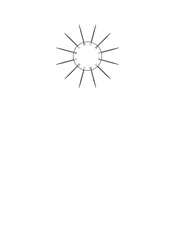
Figure 1: Classical membrane instability arises from spikes of infinitesimal area

In the matrix regularized version of the membrane theory, this instability appears as a set of flat directions in the classical theory. For example, if we have a pair of matrices with nonzero entries of the form

$$X^{1}=\left(\begin{array}[]{cc}x&0\\ 0&0\end{array}\right)\;\;\;\;\;X^{2}=\left(\begin{array}[]{cc}0&y\\ y&0\end{array}\right)$$ (3.1)

then a potential term $[X^{1},X^{2}]^{2}$ corresponds to a term $x^{2}y^{2}$. If either $x=0$ or $y=0$ then the other variable is unconstrained, giving flat directions in the moduli space of solutions to the classical equations of motion. This corresponds classically to a marginal instability in the matrix theory with $N>1$. (Note that in the previous section we distinguished matrices ${\bf X}^{i}$ from related functions $X^{i}$ by using bold font for matrices. We will henceforth drop this font distinction as long as the difference can easily be distinguished from context.)

In the quantum bosonic membrane theory, the apparent instability from the flat directions is cured because of the 0-modes of off-diagonal degrees of freedom. In the above example, for instance, if $x$ takes a large value then $y$ corresponds to a harmonic oscillator degree of freedom with a large mass. The zero point energy of this oscillator becomes larger as $x$ increases, giving an effective confining potential which removes the flat directions of the classical theory. This would seem to resolve the instability problem. Indeed, in the matrix regularized quantum bosonic membrane theory, there is a discrete spectrum of energy levels for the system of $N\times N$ matrices.

When we consider the supersymmetric theory, on the other hand, the problem reemerges. The zero point energies of the fermionic oscillators associated with the extra Grassmann degrees of freedom in the supersymmetric theory conspire to precisely cancel the zero point energies of the bosonic oscillators. This cancellation gives rise to a continuous spectrum in the supersymmetric matrix theory. This result was formally proven by de Wit, Lüscher and Nicolai in [21]. They showed that for any $\epsilon>0$ and any energy $E\in[0,\infty)$ there exists a state $\psi$ in the $N=2$ maximally supersymmetric matrix model which is normalizable ($\int|\psi|^{2}=||\psi||^{2}=1$) and which has

$$||(H-E)\psi||^{2}<\epsilon.$$

This implies that the spectrum of the supersymmetric matrix quantum mechanics theory is continuous. This result indicated that it would not be possible to have a simple interpretation of the states of the theory in terms of a discrete particle spectrum. After this work there was little further development on the supersymmetric matrix quantum mechanics theory as a theory of membranes or gravity until almost a decade later.

3.2 M-theory

The concept of M-theory has played a fairly central role in the development of the web of duality symmetries which relate the five string theories to each other and to supergravity [23, 11, 24, 25, 26]. M-theory is a conjectured eleven-dimensional theory whose low-energy limit corresponds to 11D supergravity. Although there are difficulties with constructing a quantum version of 11D supergravity, it is a well-defined classical theory with the following field content [27]:

$e^{a}_{I}$: a vielbein field (bosonic, with 44 components)
$\psi_{I}$: a Majorana fermion gravitino (fermionic, with 128 components)
$A_{IJK}$: a 3-form potential (bosonic, with 84 components).

In addition to being a local theory of gravity with an extra 3-form potential field, M-theory also contains extended objects. These consist of a two-dimensional supermembrane and a 5-brane, which couple electrically and magnetically to the 3-form field.

One way of defining M-theory is as the strong coupling limit of the type IIA string. The IIA string theory is taken to be equivalent to M-theory compactified on a circle $S^{1}$, where the radius of compactification $R$ of the circle in direction 11 is related to the string coupling $g$ through $R=g^{2/3}l_{p}=gl_{s}$, where $l_{p}$ and $l_{s}=\sqrt{\alpha^{\prime}}$ are the M-theory Planck length and the string length respectively. The decompactification limit $R\rightarrow\infty$ corresponds then to the strong coupling limit of the IIA string theory. (Note that we will always take the eleven dimensions of M-theory to be labeled $0,1,\ldots,8,9,11$; capitalized roman indices $I,J,\ldots$ denote 11-dimensional indices).

Given this relationship between compactified M-theory and IIA string theory, a correspondence can be constructed between various objects in the two theories. For example, the Kaluza-Klein photon associated with the components $g_{\mu 11}$ of the 11D metric tensor can be associated with the R-R gauge field $A_{\mu}$ in IIA string theory. The only object which is charged under this R-R gauge field in IIA string theory is the D0-brane; thus, the D0-brane can be associated with a supergraviton with momentum $p_{11}$ in the compactified direction. The membrane and 5-brane of M-theory can be associated with different IIA objects depending on whether or not they are wrapped around the compactified direction; the correspondence between various M-theory and IIA objects is given in Table 1.

Table 1: Correspondence between objects in M-theory and IIA string theory

M-theory	IIA
KK photon ($g_{\mu 11}$)	RR gauge field $A_{\mu}$
supergraviton with $p_{11}=1/R$	D0-brane
wrapped membrane	IIA string
unwrapped membrane	IIA D2-brane
wrapped 5-brane	IIA D4-brane
unwrapped 5-brane	IIA NS5-brane

3.3 The BFSS conjecture

In 1996, motivated by recent work on D-branes and string dualities, Banks, Fischler, Shenker and Susskind (BFSS) proposed that the large $N$ limit of the supersymmetric matrix quantum mechanics model (2.97) should describe all of M-theory in a light-front coordinate system [3]. Although this conjecture fits neatly into the framework of the quantized membrane theory, the starting point of BFSS was to consider M-theory compactified on a circle $S^{1}$, with a large momentum in the compact direction. As we have just discussed, when M-theory is compactified on $S^{1}$ the corresponding theory in 10D is the type IIA string theory, and the quanta corresponding to momentum in the compact direction are the D0-branes of the IIA theory. In the limits where the radius of compactification $R$ and the compact momentum $p_{11}$ are both taken to be large, this correspondence relates M-theory in the “infinite momentum frame” (IMF) to the nonrelativistic theory of many D0-branes in type IIA string theory.

The low-energy Lagrangian for a system of many type IIA D0-branes is the matrix quantum mechanics Lagrangian arising from the dimensional reduction to 0 + 1 dimensions of the 10D super Yang-Mills Lagrangian

$${\cal L}=\frac{1}{2gl_{s}}{\rm Tr}\;\left[\dot{X}^{a}\dot{X}^{a}+\frac{1}{2}[X^{a},X^{b}]^{2}+\theta^{T}(i\dot{\theta}-\Gamma_{a}[X^{a},\theta])\right]$$ (3.2)

(the gauge has been fixed to $A_{0}=0$.) The corresponding Hamiltonian is

$$H={1\over 2gl_{s}}{\rm Tr}\,\left(\dot{X}^{i}\dot{X}^{i}-{1\over 2}[X^{i},X^{j}][X^{i},X^{j}]+\theta^{T}\gamma_{i}[X^{i},\theta]\right)\,.$$ (3.3)

Using the relations $R=g^{2/3}l_{11}=gl_{s}$, we see that in string units ($2\pi l_{s}^{2}=1$) we can replace $gl_{s}=R=2\pi l_{11}^{3}$. So the Hamiltonian (3.3) arising in the matrix quantum mechanics picture is in fact precisely equivalent to the matrix membrane Hamiltonian (2.97). This connection and its possible physical significance was first pointed out by Townsend [28]. The matrix theory Hamiltonian is often written, following BFSS, in the form

$$H = \frac{R}{2}{\rm Tr}\,\left(P^{i}P^{i}-{1\over 2}[X^{i},X^{j}][X^{i},X^{j}]+\theta^{T}\gamma_{i}[X^{i},\theta]\right)$$ (3.4)

where we have rescaled $X/g^{1/3}\rightarrow X$ and written the Hamiltonian in Planck units $l_{11}=1$.

The original BFSS conjecture was made in the context of the large $N$ theory. It was later argued by Susskind that the finite $N$ matrix quantum mechanics theory should be equivalent to the discrete light-front quantized (DLCQ) sector of M-theory with $N$ units of compact momentum [29]. We describe in section (3.5) below an argument due to Seiberg and Sen which makes this connection more precise and which justifies the use of the low-energy D0-brane action in the BFSS conjecture.

While the BFSS conjecture was based on a different framework from the matrix quantization of the supermembrane theory we have discussed above, the fact that the membrane naturally appears as a coherent state in the matrix quantum mechanics theory was a substantial piece of additional evidence given by BFSS for the validity of their conjecture. Two additional pieces of evidence were given by BFSS which extended their conjecture beyond the previous work on the matrix membrane theory.

One important point made by BFSS is that the Hilbert space of the matrix quantum mechanics theory naturally contains multiple particle states. This observation, which we discuss in more detail in the following subsection, resolves the problem of the continuous spectrum discussed above. Another piece of evidence given by BFSS for their conjecture is the fact that quantum effects in matrix theory give rise to long-range interactions between a pair of gravitational quanta (D0-branes) which have precisely the correct form expected from light-front supergravity. This result was first shown by a calculation of Douglas, Kabat, Pouliot and Shenker [30]; we will discuss this result and its generalization to more general matrix theory interactions in Section 5.

3.4 Matrix theory as a second quantized theory

The classical equations of motion for a bosonic matrix configuration with the Hamiltonian (2.97) are (up to an overall constant)

$$\ddot{X}^{i}=-[[X^{i},X^{j}],X^{j}].$$ (3.5)

If we consider a block-diagonal set of matrices

$$X^{i}=\left(\begin{array}[]{cc}\hat{X}^{i}&0\\ 0&\tilde{X}^{i}\end{array}\right)$$

with first time derivatives $\dot{X}^{i}$ which are also of block-diagonal form, then the classical equations of motion for the blocks are separable

$$\ddot{\hat{X}}^{i} = -[[\hat{X}^{i},\hat{X}^{j}],\hat{X}^{j}]$$

$$\ddot{\tilde{X}}^{i} = -[[\tilde{X}^{i},\tilde{X}^{j}],\tilde{X}^{j}]$$

If we think of each of these blocks as describing a matrix theory object with center of mass

$$\hat{x}^{i}=\frac{1}{\hat{N}}{\rm Tr}\;\hat{X}^{i}$$

$$\tilde{x}^{i}=\frac{1}{\tilde{N}}{\rm Tr}\;\tilde{X}^{i}$$

then we have two objects obeying classically independent equations of motion (See Figure 2). It is straightforward to generalize this construction to a block-diagonal matrix configuration describing $k$ classically independent objects. This gives a simple indication of how matrix theory can encode, even in finite $N$ matrices, a configuration of multiple objects. In this sense it is natural to think of matrix theory as a second quantized theory from the point of view of the target space.

Figure 2: Two matrix theory objects described by block-diagonal matrices

Given the realization that matrix theory should describe a second quantized theory, the puzzle discussed above regarding the continuous spectrum of the theory is easily resolved. If there is a state in matrix theory corresponding to a single graviton of M-theory (as we will discuss in more detail in section 4.1) with $H=0$ which is roughly a localized state, then by taking two such states to have a large separation and a small relative velocity $v$ it should be possible to construct a two-body state with an arbitrarily small total energy. Since the D0-branes of the IIA theory correspond to gravitons in M-theory with a single unit of longitudinal momentum, we would therefore naturally expect to have a continuous spectrum of energies even in the theory with $N=2$. This resolves the puzzle found by de Wit, Lüscher and Nicolai in a very pleasing fashion, which suggests that matrix theory is perhaps even more powerful than string theory, which only gives a first-quantized theory in the target space.

The second quantized nature of matrix theory can also be seen naturally in the continuous membrane theory. Recall that the instability of membrane theory appears in the classical theory of a continuous membrane when we consider the possibility of long thin spikes of negligible energy, as discussed in section 3.1. In a similar fashion, it is possible for a classical smooth membrane of fixed topology to be mapped to a configuration in the target space which looks like a system of multiple distinct macroscopic membranes connected by infinitesimal tubes of negligible energy (See Figure 3). In the limit where the tubes become very small, their effect on the classical dynamics of the multiple membrane configuration disappears and we effectively have a system of multiple independent membranes moving in the target space. At the classical level, the sum of the genera of the membranes in the target space must be equal to or smaller than the genus of the single world-sheet membrane, but when quantum effects are included handles can be added to the membrane as well as removed [31]. These considerations seem to indicate that any consistent quantum theory which contains a continuous membrane in its effective low-energy theory must contain configurations with arbitrary membrane topology and must therefore be a “second quantized” theory from the point of view of the target space.

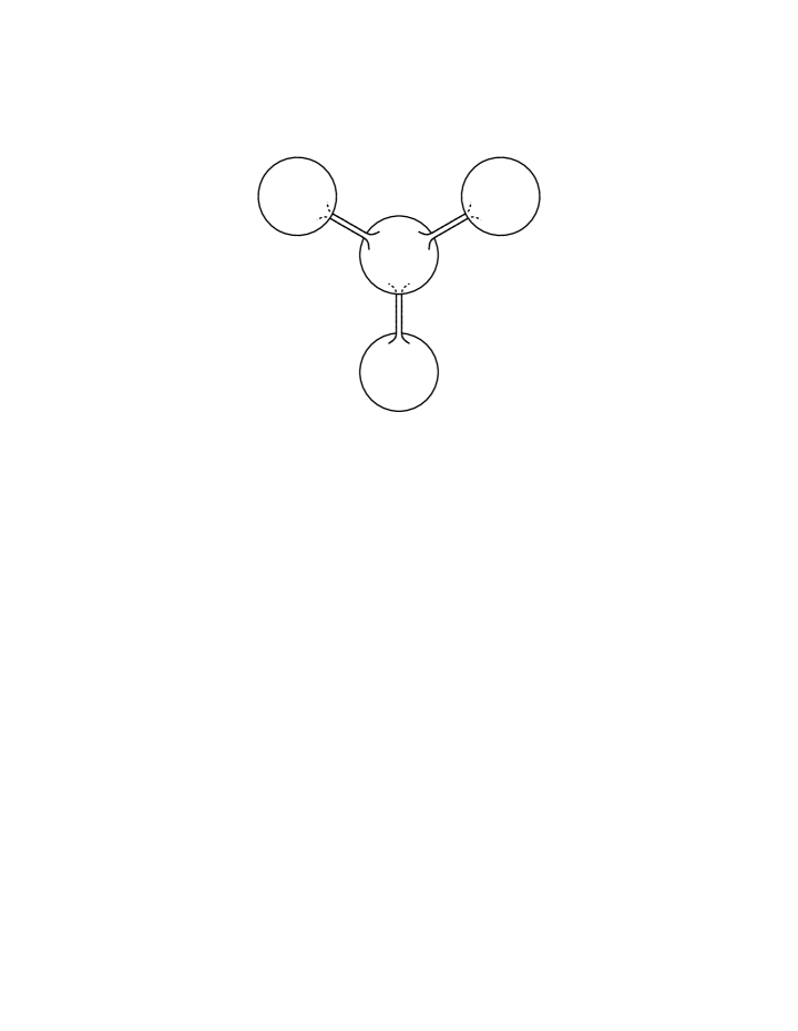
Figure 3: Membrane of fixed (spherical) topology mapped to multiple membranes connected by tubes in the target space

3.5 Matrix theory and DLCQ M-theory

A theory which has been compactified on a lightlike circle can be viewed as a limit of a theory compactified on a spacelike circle where the size of the spacelike circle becomes vanishingly small in the limit. This point of view was used by Seiberg and Sen in [32, 33] to argue that light-front compactified M-theory is described through such a limiting process by the low-energy Lagrangian for many D0-branes, and hence by matrix theory. In this section we go through this argument in detail.

Consider a space-time which has been compactified on a lightlike circle by identifying

$$\left(\begin{array}[]{c}x\\ t\end{array}\right)\sim\left(\begin{array}[]{c}x-R/\sqrt{2}\\ t+R/\sqrt{2}\end{array}\right)$$ (3.6)

This theory has a quantized momentum in the compact direction

$$P^{+}=\frac{N}{R}$$ (3.7)

The compactification (3.6) can be described as a limit of a family of spacelike compactifications

$$\left(\begin{array}[]{c}x\\ t\end{array}\right)\sim\left(\begin{array}[]{c}x-\sqrt{R^{2}/2+R_{s}^{2}}\\ t+R/\sqrt{2}\end{array}\right)$$ (3.8)

parameterized by the size $R_{s}\rightarrow 0$ of the spacelike circle, which is taken to vanish in the limit.

The system satisfying (3.8) is related through a boost to a system with the identification

$$\left(\begin{array}[]{c}x^{\prime}\\ t^{\prime}\end{array}\right)\sim\left(\begin{array}[]{c}x^{\prime}-R_{s}\\ t^{\prime}\end{array}\right)$$ (3.9)

where

$$\left(\begin{array}[]{c}x^{\prime}\\ t^{\prime}\end{array}\right)=\left(\begin{array}[]{cc}\frac{1}{\sqrt{1-\beta^{2}}}&\frac{\beta}{\sqrt{1-\beta^{2}}}\\ \frac{\beta}{\sqrt{1-\beta^{2}}}&\frac{1}{\sqrt{1-\beta^{2}}}\end{array}\right)\left(\begin{array}[]{c}x\\ t\end{array}\right)$$ (3.10)

The boost parameter $\beta$ is given by

$$\beta=\frac{1}{\sqrt{1+\frac{2R_{s}^{2}}{R^{2}}}}\equiv 1-\frac{R_{s}^{2}}{R^{2}}.$$ (3.11)

In the context of matrix theory we are interested in understanding M-theory compactified on a lightlike circle. This is related through the above limiting process to a family of spacelike compactifications of M-theory, which we know can be identified with the IIA string theory. At first glance, it may seem that the limit we are considering here is difficult to analyze from the IIA point of view. The IIA string coupling and string length are related to the compactification radius and 11D Planck length as usual by

$$g = (\frac{R_{s}}{l_{11}})^{3/2}$$ (3.12)

$$l_{s}^{2} = \frac{l_{11}^{3}}{R_{s}}$$

Thus, in the limit $R_{s}\rightarrow\infty$ the string coupling $g$ becomes small as desired; the string length $l_{s}$, however, goes to $\infty$. Since $l_{s}^{2}=\alpha^{\prime}$, this corresponds to a limit of vanishing string tension. Such a limiting theory is very complicated and would not seem to provide a useful alternative description of the theory.

Let us consider, however, how the energy of the states we are interested in behaves in the class of limiting theories with spacelike compactification. If we want to describe the behavior of a state which has light-front energy $P^{-}$ and compact momentum $P^{+}=N/R$ then the spatial momentum in the theory with spatial $R_{s}$ compactification is $P^{\prime}=N/R_{s}$. The energy in the spatially compactified theory is

$$E^{\prime}=N/R_{s}+\Delta E,$$ (3.13)

where $\Delta E$ has the energy scale we are interested in understanding. The term $N/R_{s}$ in the energy is simply the mass-energy of the $N$ D0-branes which correspond to the momentum in the compactified M-theory direction. Relating back to the near lightlike compactified theory we have

$$\left(\begin{array}[]{c}P\\ E\end{array}\right) = \left(\begin{array}[]{cc}\frac{1}{\sqrt{1-\beta^{2}}}&-\frac{\beta}{\sqrt{1-\beta^{2}}}\\ -\frac{\beta}{\sqrt{1-\beta^{2}}}&\frac{1}{\sqrt{1-\beta^{2}}}\end{array}\right)\left(\begin{array}[]{c}P^{\prime}\\ E^{\prime}\end{array}\right)$$ (3.20)

so

$$P^{-}=\frac{1}{\sqrt{2}}(E-P)=\frac{1}{\sqrt{2}}\frac{1+\beta}{\sqrt{1-\beta^{2}}}\Delta E\approx\frac{R}{R_{s}}\Delta E$$ (3.21)

As a result we see that the energy $\Delta E$ of the IIA configuration needed to approximate the light-front energy $P^{-}$ is given by

$$\Delta E\approx P^{-}\frac{R_{s}}{R}$$ (3.22)

We know that the string scale $1/l_{s}$ becomes small as $R_{s}\rightarrow 0$. We can compare the energy scale of interest to this string scale, however, and find

$$\frac{\Delta E}{(1/l_{s})}=\frac{P^{-}}{R}R_{s}l_{s}=\frac{P^{-}}{R}\sqrt{R_{s}l_{11}^{3}}$$ (3.23)

This ratio vanishes in the limit $R_{s}\rightarrow 0$, which implies that although the string scale vanishes, the energy scale of interest is smaller still. Thus, it is reasonable to study the lightlike compactification through a limit of spatial compactifications in this fashion.

To make the correspondence between the light-front compactified theory and the spatially compactified limiting theories more transparent, we perform a change of units to a new Planck length $\tilde{l}_{11}$ in the spatially compactified theories in such a way that the energy of the states of interest is independent of $R_{s}$. For this condition to hold we must have

$$\Delta E\tilde{l}_{11}=P^{-}\frac{R_{s}{l}_{11}^{2}}{R\tilde{l}_{11}}$$ (3.24)

where $E,R$ and $P^{-}$ are independent of $R_{s}$ and all units have been explicitly included. This requires us to keep the quantity

$$\frac{R_{s}}{\tilde{l}_{11}^{2}}$$ (3.25)

fixed in the limiting process. Thus, in the limit $\tilde{l}_{11}\rightarrow 0$.

We can now summarize the discussion with the following story: to describe the sector of M-theory corresponding to light-front compactification on a circle of radius $R$ with light-front momentum $P^{+}=N/R$ we may consider the limit $R_{s}\rightarrow 0$ of a family of IIA configurations with $N$ D0-branes where the string coupling and string length

$$\tilde{g} = (R_{s}/\tilde{l}_{11})^{3/2}\rightarrow 0$$

$$\tilde{l}_{s} = \sqrt{\tilde{l}_{11}^{3}/R_{s}}\rightarrow 0$$ (3.26)

are defined in terms of a Planck length $\tilde{l}_{11}$ and compactification length $R_{s}$ which satisfy

$$R_{s}/\tilde{l}_{11}^{2}=R/l_{11}^{2}$$ (3.27)

All transverse directions scale normally through

$$\tilde{x}^{i}/\tilde{l}_{11}=x^{i}/l_{11}$$ (3.28)

To give a very concrete example of how this limiting process works, let us consider a system with a single unit of longitudinal momentum

$$P^{+}=\frac{1}{R}$$ (3.29)

We know that in the corresponding IIA theory, we have a single D0-brane whose Lagrangian has the Born-Infeld form

$${\cal L}=-\frac{1}{\tilde{g}\tilde{l}_{s}}\sqrt{1-\dot{\tilde{x}}^{i}\dot{\tilde{x}}^{i}}$$ (3.30)

Expanding the square root we have

$${\cal L}=-\frac{1}{\tilde{g}\tilde{l}_{s}}\left(1-\frac{1}{2}\dot{\tilde{x}}^{i}\dot{\tilde{x}}^{i}+{\cal O}(\dot{\tilde{x}}^{4})\right).$$ (3.31)

Replacing $\tilde{g}\tilde{l}_{s}\rightarrow R_{s}$ and $\tilde{x}\rightarrow x\tilde{l}_{11}/l_{11}$ gives

$${\cal L}=-\frac{1}{R_{s}}+\frac{1}{2R}\dot{x}^{i}\dot{x}^{i}+{\cal O}(R_{s}/R).$$ (3.32)

Thus, we see that all the higher order terms in the Born-Infeld action vanish in the $R_{s}\rightarrow 0$ limit. The leading term is the D0-brane energy $1/R_{s}$ which we subtract to compare to the M-theory light-front energy $P^{-}$. Although we do not know the full form of the nonabelian Born-Infeld action describing $N$ D0-branes in IIA, it is clear that an analogous argument shows that all terms in this action other than those in the nonrelativistic supersymmetric matrix theory action will vanish in the limit $R_{s}\rightarrow 0$.

This argument apparently demonstrates that matrix theory gives a complete description of the dynamics of DLCQ M-theory. There are several caveats which should be taken into account, however, with respect to this discussion. First, in order for this argument to be correct, it is necessary that there exists a well-defined theory with the properties expected of M-theory, and that there exist a well-defined IIA string theory which arises as the compactification of M-theory. Neither of these statements is at this point definitely established. Thus, this argument must be taken as contingent upon the definition of these theories. Second, although we know that 11D supergravity arises as the low-energy limit of M-theory, this argument does not necessarily indicate that matrix theory describes DLCQ supergravity in the low-energy limit. It may be that to make the connection to supergravity it is necessary to deal with subtleties of the large $N$ limit.

In the remainder of these lectures we will discuss some more explicit approaches to connecting matrix theory with supergravity. In particular, we will see how far it is possible to go in demonstrating that 11D supergravity arises from calculations in the finite $N$ version of matrix theory, which is a completely well-defined theory. In the last sections we will return to a more general discussion of the status of matrix theory.

4 M-theory objects from matrix theory

In this section we discuss how the matrix theory degrees of freedom can be used to construct the various objects of M-theory: the supergraviton, supermembrane and 5-brane. We discuss each of these objects in turn in subsections 4.1, 4.2, 4.3, after which we give a general discussion of the structure of extended objects and their charges in subsection 4.4

4.1 Supergravitons

Since in DLCQ M-theory there should be a pointlike state corresponding to a longitudinal graviton with $p^{+}=N/R$ and arbitrary transverse momentum $p^{i}$, we expect from the massless condition $m^{2}=-p^{I}p_{I}=0$ that such an object will have matrix theory energy

$$E=\frac{p_{i}^{2}}{2p^{+}}$$

We discuss such states first classically and then in the quantum theory.

4.1.1 Classical supergravitons

The classical matrix theory potential is $-[X^{i},X^{j}]^{2}$, from which we have the classical equations of motion

$$\ddot{X}^{i}=-[[X^{i},X^{j}],X^{j}].$$

One simple class of solutions to these equations of motion can be found when the matrices minimize the potential at all times and therefore all commute. Such solutions are of the form

$$X^{i}=\left(\begin{array}[]{cccc}x^{i}_{1}+v^{i}_{1}t&0&0&\ddots\\ 0&x^{i}_{2}+v^{i}_{2}t&\ddots&0\\ 0&\ddots&\ddots&0\\ \ddots&0&0&x^{i}_{N}+v^{i}_{N}t\end{array}\right)$$

This corresponds to a classical $N$-graviton solution, where each graviton has

$$p_{a}^{+}=1/R\;\;\;\;\;p^{i}_{a}=v^{i}_{a}/R\;\;\;\;\;E_{a}=v_{a}^{2}/(2R)=(p_{a}^{i})^{2}/2p^{+}$$

A single classical graviton with $p^{+}=N/R$ can be formed by setting

$$x_{1}^{i}=\cdots=x_{N}^{i},\;\;\;\;\;v_{1}^{i}=\cdots=v_{N}^{i}$$

so that the trajectories of all the components are identical. Although this may seem like a very simple model for a graviton, it is precisely such matrix configurations which are used as a background in most computations of quantum effects in matrix theory corresponding to gravitational interactions, as will be discussed further in the following.

4.1.2 Quantum supergravitons

The picture of a supergraviton in quantum matrix theory is somewhat more subtle than the simple classical picture just discussed. Let us first consider the case of a single supergraviton with $p^{+}=1/R$. This corresponds to the U(1) case of the super Yang-Mills quantum mechanics theory. The Hamiltonian is simply

$$H=\frac{1}{2R}\dot{X}^{2}$$

since all commutators vanish in this theory. The bosonic part of the theory is simply a free nonrelativistic particle. In the fermionic sector there are 16 spinor variables with anticommutation relations

$$\{\theta_{\alpha},\theta_{\beta}\}=\delta_{\alpha\beta}.$$

By using the standard trick of writing these as 8 fermion creation and annihilation operators

$$\theta_{i}^{\pm}=\frac{1}{\sqrt{2}}(\theta_{i}\pm\theta_{i+8})\;\;\;\;\;\;1\leq i\leq 8$$

we see that the Hilbert space for the fermions is a standard fermion Fock space of dimension $2^{8}=256$. Indeed, this is precisely the number of states needed to represent all the polarization states of the graviton (44), the antisymmetric 3-tensor field (84) and the gravitino (128). For details of how the polarization states are represented in terms of the fermionic Fock space, see [2, 34].

The case when $N>1$ is much more subtle. We can factor out the overall $U(1)$ so that every state in the $SU(N)$ quantum mechanics theory has 256 corresponding states in the full theory. For the matrix theory conjecture to be correct, as BFSS pointed out, it should then be the case that for every $N$ there exists a unique threshold bound state in the $SU(N)$ theory with $H=0$. As mentioned before, no definitive answer as to the existence of such a state was given in the early work on matrix theory. This result was finally proven by Sethi and Stern for $N=2$ in [22]. Progress towards proving the result for arbitrary values of $N$ was made in [35, 36, 37], and the result for a general gauge group was given in [38] (see also [39]).

4.2 Membranes

In this section we discuss the description of M-theory membranes in terms of the matrix quantum mechanics degrees of freedom. It is clear from the derivation of matrix theory as a regularized supermembrane theory that there must be matrix configurations which in the large $N$ limit give arbitrarily good descriptions of any membrane configuration. It is instructive, however, to study in detail the structure of such membrane configurations. In subsection 4.2.1 we discuss the significance of the matrix representation of membranes in the language of type IIA D0-branes. In subsection 4.2.2 we discuss in some detail how a spherical membrane can be very accurately described by matrices even with small values of $N$. In subsection 4.2.3 we discuss higher genus matrix membranes. In subsection 4.2.4 we discuss noncompact matrix membranes, and finally in subsection 4.2.5 we discuss M-theory membranes which are wrapped on the longitudinal direction and appear as strings in the IIA theory.

4.2.1 D2-branes from D0-branes

As we have mentioned, it is clear from inverting the matrix membrane regularization procedure that smooth membranes can be approximated by finite size matrices. This construction may seem less natural in the language of type IIA string theory, where it corresponds to a construction of a IIA D2-brane out of the degrees of freedom describing a system of $N$ D0-branes. In fact, however, the fact that this construction is possible is simply the T-dual of the familiar statement that D0-branes are described by the magnetic flux of the gauge field living on a set of $N$ D2-branes [40]. Both of these statements can in turn be seen by performing T-duality on a diagonally wrapped D1-brane on a 2-torus.

To see this explicitly, consider a set of $N$ D2-branes on a torus $T^{2}$ with $k$ units of magnetic flux

$$\frac{1}{2\pi}\int F=k$$ (4.1)

Under a T-duality transformation on one direction of the torus, the gauge field component $A_{2}$ is replaced by an infinite matrix

$$X^{2}=i\partial_{2}+A_{2}$$

representing a transverse scalar field for a set of $N$ D1-branes living on the dual torus $(T^{2})^{*}$. These matrices are infinite because they contain information about winding strings connecting the infinite number of copies of each brane which live on the infinite covering space of the dual torus. (This construction is described in more detail in section 6.1.) This T-dual configuration corresponds to a single D-string which is diagonally wound $N$ times around the $x^{1}$ direction and $k$ times around the $x^{2}$ direction; this can be seen from the fact that the T-dual of (4.1) is $\partial_{1}X^{2}=(kL_{2}^{*}/NL_{1}){\hbox to0.0pt{1\hss}\hskip 1.6pt\hbox{1}}$. Since under T-duality in the $x^{2}$ direction a D1-brane wrapped in the $x^{2}$ direction becomes a D0-brane, we can identify the flux (4.1) with $k$ D0-branes in the original theory.

Further T-dualizing in the direction $x^{1}$, we replace

$$X^{1}=i\partial_{1}+A_{1}.$$

where $X^{1},X^{2}$ are now infinite matrices describing transverse fields of a system of $N$ D0-branes on the dual torus $(T^{2})^{**}$. When the normalization constants are treated carefully, the flux condition (4.1) now becomes the condition on the D0-brane matrices

$${\rm Tr}\;[X^{1},X^{2}]=\frac{iAk}{2\pi}$$ (4.2)

where $A$ is the area of the dual torus. Since the T-dual in the $x^{1}$ direction of the D-string wrapped in the $x^{2}$ direction is a D2-brane, we interpret $k$ in (4.2) as the D2-brane charge of a system of $N$ D0-branes.

This construction can be interpreted more generally, so that in general a pair of matrices $X^{a},X^{b}$ describing a D0-brane configuration satisfying

$${\rm Tr}\;[X^{a},X^{b}]=\frac{iA}{2\pi}$$ (4.3)

should be interpreted as giving rise to a piece of a D2-brane of area $A$. Of course, for finite matrices the trace of the commutator must vanish. This is simply a consequence of the fact that the net D2-brane charge of any compact object must vanish. However, not only is it possible to have a nonzero membrane charge when the matrices are infinite, but it is also possible to treat (4.3) as a local expression by restricting the trace to a subset of the diagonal elements. We will see a specific example of this in the next subsection. The local relation (4.3) will also be useful in constructing higher moments of the membrane charge, which can be nonzero even for finite size configurations, as we shall discuss later.

4.2.2 Spherical membranes

One extremely simple example of a membrane configuration which can be approximated very well even at finite $N$ by simple matrix configurations is the symmetric spherical membrane [41]. Imagine that we wish to construct a membrane embedded in an isotropic sphere

$$x_{1}^{2}+x_{2}^{2}+x_{3}^{2}=r^{2}$$

in the first three dimensions of ${R}^{11}$. The embedding functions for such a continuous membrane can be written as linear functions

$$X^{i}=r\xi^{i}\;\;\;\;\;\;1\leq i\leq 3$$

of the three Euclidean coordinates $\xi^{i}$ on the spherical world-volume. Using the matrix-membrane correspondence (2.51) we see that the matrix approximation to this membrane will be given by the $N\times N$ matrices

$${\bf X}^{i}=\frac{2r}{N}J^{i}\;\;\;\;\;\;1\leq i\leq 3$$ (4.4)

where $J^{i}$ are the generators of $SU(2)$ in the $N$-dimensional representation.

It is quite interesting to see how many of the geometrical and physical properties of the sphere can be extracted from the algebraic structure of these matrices, even for small values of $N$. We list here some of these properties.

i) Spherical locus: The matrices (4.4) satisfy

$${\bf X}_{1}^{2}+{\bf X}_{2}^{2}+{\bf X}_{3}^{2}=\frac{4r^{2}}{N^{2}}C_{2}(N){\hbox to0.0pt{1\hss}\hskip 1.6pt\hbox{1}}=r^{2}(1-1/N^{2}){\hbox to0.0pt{1\hss}\hskip 1.6pt\hbox{1}}$$

where $C_{2}(N)=(N^{2}-1)/4$ is the quadratic Casimir of $SU(2)$ in the $N$-dimensional representation. This shows that the D0-branes are in a noncommutative sense “localized” on a sphere of radius $r+{\cal O}(1/N^{2})$.

ii) Rotational invariance: The matrices (4.4) satisfy

$$R_{ij}{\bf X}_{j}=U(R)\cdot{\bf X}_{i}\cdot U(R^{-1})$$

where $R\in SO(3)$ and $U(R)$ is the $N$-dimensional representation of $R$. Thus, the spherical matrix configuration is rotationally invariant up to a gauge transformation.

iii) Spectrum: The matrix ${\bf X}^{3}=2rJ_{3}/N$ (as well as the other matrices) has a spectrum of eigenvalues which are uniformly distributed in the interval $[-r,r]$. This is precisely the correct distribution if we imagine a perfectly symmetric sphere with D0-branes distributed uniformly on its surface and project this distribution onto a single axis.

iv) Local membrane charge: As discussed above, the expression (4.3) gives an area for a piece of a membrane described by a pair of matrices. We can use this formula to check the interpretation of the matrix sphere. We do this by computing the membrane charge in the 1-2 plane of the half of the configuration with eigenvalues $X^{3}>0$. This should correspond to the projected area of the “upper hemisphere” of the sphere. We compute

$$A_{h}=-2\pi i{\rm Tr}_{1/2}\;[{\bf X}^{1},{\bf X}^{2}]$$

where the trace is restricted to the set of eigenvalues where $X^{3}>0$ in the standard representation. This is possible since $[{\bf X}^{1},{\bf X}^{2}]\sim{\bf X}^{3}$. We find

$$A_{h}=2\pi\frac{4}{N^{2}}r^{2}{\rm Tr}_{1/2}\;J_{3}=\pi r^{2}(1+{\cal O}(1/N^{2}))$$

thus, we find precisely the expected area of the projected hemisphere.

v) Energy: In M-theory we expect the tension energy of a (momentarily) stationary membrane sphere to be

$$e=\frac{4\pi r^{2}}{(2\pi)^{2}l_{11}^{3}}=\frac{r^{2}}{\pi l_{11}^{3}}$$

Using $p^{I}p_{I}=-e^{2}$ we see that the light-front energy should be

$$E=\frac{e^{2}}{2p^{+}}$$ (4.5)

in 11D Planck units. Let us compute the matrix membrane energy. It is given by

$$E=-\frac{1}{4R}[{\bf X}^{i},{\bf X}^{j}]^{2}=\frac{2r^{4}}{NR}+{\cal O}(N^{-3})$$

in string units. This is easily seen to agree with (4.5).

It is also straightforward to verify that the equations of motion for the membrane are correctly reproduced in matrix theory.

Thus, we see that many of the geometrical and physical properties of the membrane can be extracted from algebraic information about the structure of the appropriate membrane configuration. The discussion we have carried out here has only applied to the simple case of the rotationally invariant spherically embedded membrane. It is straightforward to extend the discussion to a membrane of spherical topology and arbitrary shape, however, simply by using the matrix-membrane correspondence (2.51) to construct matrices approximating an arbitrary smooth spherical membrane. We now turn to the question of membranes with non-spherical topology.

4.2.3 Higher genus membranes

So far we have only discussed membranes of spherical topology. It is possible to describe compact membranes of arbitrary genus by generalizing this construction, although an explicit construction is only known for the sphere and torus. In this section we give a brief description of the matrix torus, following the work of Fairlie, Fletcher and Zachos [42, 43, 44].

We consider a torus defined by two coordinates $x_{1},x_{2}\in[0,2\pi]$ with symplectic form $\omega_{ij}=\epsilon_{ij}/\pi$ corresponding to a total volume $\int d^{2}x\;\omega=4\pi$ as in the case of the sphere discussed in section 2.4. As in the case of the sphere we wish to find a map from functions on the torus to matrices which is compatible with the correspondence

$$\{\cdot,\cdot\}\leftrightarrow{-iN\over 2}[\cdot,\cdot]\;\;\;\;\;\;\;\;\;\;{1\over 4\pi^{2}}\int d^{2}x\leftrightarrow\frac{1}{N}{\rm Tr}\,$$ (4.6)

A natural (complex) basis for the functions on $T^{2}$ is given by the Fourier modes

$$y_{nm}(x_{1},x_{2})=e^{inx_{1}+imx_{2}}$$ (4.7)

The real functions on $T^{2}$ are given by the linear combinations

$$\frac{1}{2}\left(y_{nm}+y_{-n\,-m}\right),\;\;\;\;\;\frac{-i}{2}\left(y_{nm}-y_{-n\,-m}\right).$$ (4.8)

The Poisson bracket algebra of the functions $y_{nm}$ is

$$\{y_{nm},y_{n^{\prime}m^{\prime}}\}=-\pi(nm^{\prime}-mn^{\prime})y_{n+n^{\prime},m+m^{\prime}}$$ (4.9)

To describe the matrix approximations for these functions we use the ’t Hooft matrices

$$U=\pmatrix{1&&&&\cr&q&&&\cr&&q^{2}&&\cr&&&\ddots&\cr&&&&q^{N-1}}$$ (4.10)

and

$$V=\pmatrix{&1&&&\cr&&1&&\cr&&&\ddots&\cr&&&&1\cr 1&&&&}$$ (4.11)

where

$$q=e^{2\pi i\over N}.$$ (4.12)

The matrices $U,V$ satisfy

$$UV=q^{-1}VU.$$ (4.13)

In terms of these matrices we can define

$$Y_{nm}=q^{nm/2}U^{n}V^{m}=q^{-nm/2}V^{m}U^{n}$$ (4.14)

so that the matrix approximation to an arbitrary function

$$f(x_{1},x_{2})=\sum_{n,m}c_{nm}y_{nm}(x_{1},x_{2})$$ (4.15)

is given by

$$F=\sum_{n,m}c_{nm}Y_{nm}.$$ (4.16)

By computing

$$[Y_{nm},Y_{n^{\prime}m^{\prime}}] = (q^{(mn^{\prime}-nm^{\prime})/2}-q^{(nm^{\prime}-mn^{\prime})/2})Y_{n+n^{\prime},m+m^{\prime}}$$

$$\rightarrow \frac{2\pi i}{N}(mn^{\prime}-nm^{\prime})Y_{n+n^{\prime},m+m^{\prime}}$$

We see that for fixed $n,m,n^{\prime},m^{\prime}$ in the large $N$ limit the matrix commutation relations correctly reproduce (4.9) just as in the case of the sphere.

As a concrete example let us consider embedding a torus into ${R}^{4}\subset{R}^{9}$ so that the membrane fills the locus of points satisfying

$$X_{1}^{2}+X_{2}^{2}=r^{2}\;\;\;\;\;\;\;\;\;\;X_{3}^{2}+X_{4}^{2}=s^{2}.$$ (4.17)

Such a membrane configuration can be realized through the following matrices

$${\bf X}_{1} = \frac{r}{2}(U+U^{\dagger})$$

$${\bf X}_{2} = \frac{-ir}{2}(U-U^{\dagger})$$ (4.18)

$${\bf X}_{3} = \frac{s}{2}(V+V^{\dagger})$$

$${\bf X}_{4} = \frac{-is}{2}(V-V^{\dagger})$$

It is straightforward to check that this matrix configuration has geometrical properties analogous to those of the matrix membrane sphere discussed in the previous subsection. In particular, the equation (4.17) is satisfied identically as a matrix equation. Note, however that this configuration is not gauge invariant under $U(1)$ rotations in the 12 and 34 planes—only under a ${Z}_{N}$ subgroup of each of these $U(1)$’s.

4.2.4 Infinite membranes

So far we have discussed compact membranes, which can be described in terms of finite-size $N\times N$ matrices. In the large $N$ limit it is also possible to construct membranes with infinite spatial extent. The matrices $X^{i}$ describing such configurations are infinite-dimensional matrices which correspond to operators on a Hilbert space. Infinite membranes are of particular interest because they can be BPS states which solve the classical equations of motion of matrix theory. Extended compact membranes cannot be static solutions of the equations of motion since their membrane tension always causes them to contract and oscillate, as in the case of the spherical membrane.

The simplest infinite membrane is the flat planar membrane corresponding in IIA theory to an infinite D2-brane. This solution can be found by looking at the limit of the spherical membrane at large radius. It is simpler, however, to simply directly construct the solution by regularizing the flat membrane of M-theory. As in the other cases we have studied, we wish to quantize the Poisson bracket algebra of functions on the brane. Functions on the infinite membrane can be described in terms of two coordinates $x_{1},x_{2}$ with a symplectic form $\omega_{ij}=\epsilon_{ij}$ giving a Poisson bracket

$$\{f(x_{1},x_{2}),g(x_{1},x_{2})\}=\partial_{1}f\partial_{2}g-\partial_{1}g\partial_{2}f.$$ (4.19)

This algebra of functions can be “quantized” to the algebra of operators generated by $Q,P$ satisfying

$$[Q,P]=\frac{i\epsilon^{2}}{2\pi}{\hbox to0.0pt{1\hss}\hskip 1.6pt\hbox{1}}$$ (4.20)

where $\epsilon$ is a constant parameter. As usual in the quantization process there are operator-ordering ambiguities which must be resolved in determining a general map from functions expressed as polynomials in $x_{1},x_{2}$ to operators expressed as polynomials of $Q,P$.

This gives a map from functions on ${R}^{2}$ to operators which allows us to describe fluctuations around a flat membrane geometry with a single unit of $P^{+}=1/R$ in each region of area $\epsilon^{2}$ on the membrane. Configurations of this type were discussed in the original BFSS paper [3] and their existence used as additional evidence for the validity of their conjecture. Note that this configuration only makes sense in the large $N$ limit.

In addition to the flat membrane solution there are other infinite membranes which are static solutions of M-theory in flat space. In particular, there are BPS solutions corresponding to membranes which are holomorphically embedded in ${C}^{4}={R}^{8}\subset{R}^{9}$. These are static solutions of the membrane equations of motion. Finding a matrix theory description of such membranes is possible but involves some somewhat subtle issues related to choosing a regularization which preserves the complex structure of the brane. The details of this construction for a general holomorphic membrane are discussed in [45].

4.2.5 Wrapped membranes as matrix strings

So far we have discussed M-theory membranes which are unwrapped in the longitudinal direction and which therefore appear as D2-branes in the IIA language of matrix theory. It is also possible to describe wrapped M-theory membranes which correspond to strings in the IIA picture. The charge in matrix theory which measures the number of strings present is proportional to

$$\frac{i}{R}{\rm Tr}\;\left([X^{i},X^{j}]\dot{X}^{j}+[[X^{i},\theta^{\dot{\alpha}}],\theta^{\dot{\alpha}}]\right)$$ (4.21)

This result can be understood in several ways. It was found in [46] as a central charge in the matrix theory SUSY algebra corresponding to string charge; we will discuss this algebra further in the subsection 4.4. An intuitive way of understanding why (4.21) measures string charge is by a T-duality argument analogous to that used in 4.2.1 to derive the D2-brane charge of a system of D0-branes. If we compactify on a 2-torus in the $i$ and $j$ directions, the D0-branes become D2-branes and the bosonic part of (4.21) becomes

$$\frac{1}{R}F^{ij}F_{j0}.$$ (4.22)

This is the part of the energy-momentum tensor usually referred to as the Poynting vector in the 4D theory, and which describes momentum in the $i$ direction. Such momentum is of course T-dual to string winding in the original picture, so we understand the identification of the original charge (4.21) as counting fundamental IIA strings corresponding to wound M-theory membranes. Configurations with nonzero values of this charge were considered by Imamura in [47].

To realize a classical configuration in matrix theory which contains fundamental strings it is clear from the form of the charge that we need to construct configuration with local membrane charge extended in a pair of directions $X^{i},X^{j}$ and to give the D0-branes velocity in the $X^{j}$ direction. For example, we could consider an infinite planar membrane (as discussed in the previous subsection) sliding along itself according to the equation

$$X^{1} = Q+t{\hbox to0.0pt{1\hss}\hskip 1.6pt\hbox{1}}$$ (4.23)

$$X^{2} = P$$ (4.24)

This corresponds to an M-theory membrane which has a projection onto the $X^{1},X^{2}$ plane and which wraps around the compact direction as a periodic function of $X^{1}$ so that the IIA system contains a D2-brane with infinite strings extended in the $X^{2}$ direction since

$$\dot{X}^{1}[X^{1},X^{2}]\sim{\hbox to0.0pt{1\hss}\hskip 1.6pt\hbox{1}}.$$ (4.25)

Another example of a matrix theory system containing fundamental strings can be constructed by spinning the torus from (4.18) in the 12 plane to stabilize it. This gives the system some fundamental strings wrapped around the 34 circle. By taking the radius $r$ to be very small we can construct a configuration of a single fundamental string wrapped in a circle of radius $s$. As $s\rightarrow\infty$ this becomes an infinite fundamental string.

It is interesting to note that there is no classical matrix theory solution corresponding to a classical string which is truly 1-dimensional and has no local membrane charge. This follows from the appearance of the commutator $[X^{i},X^{j}]$ in the string charge, which vanishes unless the matrices describe a configuration with at least two dimensions of spatial extent. We can come very close to a 1-dimensional classical string configuration by considering a one-dimensional array of D0-branes at equal intervals on the $X^{1}$ axis

$$X^{1}=a\left(\begin{array}[]{ccccc}\ddots&\ddots&\ddots&&\\ \ddots&1&0&\ddots&\\ \ddots&0&0&0&\ddots\\ \ddots&\ddots&0&-1&\ddots\\ &&\ddots&\ddots&\ddots\end{array}\right)$$ (4.26)

We can now construct an excitation of the off-diagonal elements of $X^{2}$ corresponding to a string threading through the line of D0-branes

$$X^{2}=b\left(\begin{array}[]{ccccc}\ddots&\ddots&\ddots&&\\ \ddots&0&e^{i\omega t}&\ddots&\\ \ddots&e^{-i\omega t}&0&e^{i\omega t}&\ddots\\ \ddots&\ddots&e^{-i\omega t}&0&\ddots\\ &&\ddots&\ddots&\ddots\end{array}\right)$$ (4.27)

where $\omega=a$. In the classical theory, this configuration can have arbitrary string charge. If the mode (4.27) is quantized then the string charge is quantized in the correct units. This string is almost 1-dimensional but has a small additional extent in the $X^{2}$ direction corresponding to the extra dimension of the M-theory membrane. From the M-theory point of view this extra dimension must appear because the membrane cannot have momentum in a direction parallel to its direction of extension since it has no internal degrees of freedom. Thus, the momentum in the compact direction represented by the D0-branes must appear on the membrane as a fluctuation in some transverse direction.

4.3 5-branes

The M-theory 5-brane can appear in two possible guises in type IIA string theory. If the 5-brane is wrapped around the compact direction it becomes a D4-brane in the IIA theory, while if it is unwrapped it appears as an NS 5-brane. We will refer to these two configurations as “longitudinal” and “transverse” 5-branes in matrix theory. We begin by discussing the transverse 5-brane.

A priori, one might think that it should be possible to see both types of 5-branes in matrix theory. Several calculations, however, indicate that the transverse 5-brane does not carry a conserved charge which can be described in terms of the matrix degrees of freedom. In principle, if this charge existed we would expect it to appear both in the supersymmetry algebra of matrix theory (discussed in the next subsection) and in the set of supergravity currents whose interactions are described by perturbative matrix theory calculations (discussed in section 5.1.2). In fact, no charge or current with the proper tensor structure for a transverse 5-brane appears in either of these calculations.

One way of understanding this apparent puzzle is by comparing to the situation for D-branes in light-front string theory [46]. Due to the Virasoro constraints, strings in the light-front formalism must have Neumann boundary conditions in both the light-front directions $X^{+},X^{-}$. Thus, in light-front string theory there are no transverse D-branes which can be used as boundary conditions for the string. A similar situation holds for membranes in M-theory, which can end on M5-branes. The boundary conditions on the bosonic membrane fields which can be derived from the action (2.22) state that

$$(\bar{h}h^{ab}\partial_{b}X^{i})\delta X^{i}=0$$ (4.28)

Combined with the Virasoro-type constraint

$$\partial_{a}X^{-}=\dot{X}^{i}\partial_{a}X^{i}$$ (4.29)

we find that, just as in the string theory case, membranes must have Neumann boundary conditions in the light-front directions.

These considerations would seem to lead to the conclusion that transverse 5-branes simply cannot be constructed in matrix theory. On the other hand, it was argued in [48] that there may be a way to construct a transverse 5-brane using S-duality, at least when the theory has been compactified on a 3-torus. To construct an infinite extended transverse 5-brane in this fashion would require performing an S-duality on $(3+1)$-dimensional ${\cal N}=4$ supersymmetric Yang-Mills theory with gauge group $U(\infty)$, which is a poorly understood procedure to say the least. In [49], however, a finite size transverse 5-brane with geometry $T^{3}\times S^{2}$ was constructed using S-duality of the four-dimensional $U(N)$ with finite $N$. Furthermore, it was shown that this object couples correctly to the supergravity fields even in the absence of an explicit transverse 5-brane charge. This seems to indicate that transverse 5-branes in matrix theory can be constructed locally, but that they are essentially solitonic objects and do not carry independent conserved quantum numbers. It would be nice to have a more explicit construction of a general class of such finite size transverse 5-branes, particular in the noncompact version of matrix theory.

We now turn to the wrapped, or “longitudinal”, M5-brane which we will refer to as the “L5-brane”. This object appears as a D4-brane in the IIA theory. An infinite D4-brane was considered as a matrix theory background in [50] by including extra fields corresponding to strings stretching between the D0-branes of matrix theory and the background D4-brane. As in the case of the membrane, however, we would like to find a way to explicitly describe a dynamical L5-brane using the matrix degrees of freedom. Just as for the D2-brane, it may be surprising that a D4-brane can be constructed from a configuration of D0-branes. This can be seen from the same type of T-duality argument we used for the D2-brane in 4.2.1. By putting D4-branes and D0-branes on a torus $T^{4}$ we find that the charge-volume relation analogous to (4.2) for a D4-brane is [48, 6]

$${\rm Tr}\;\epsilon_{ijkl}X^{i}X^{j}X^{k}X^{l}=\frac{V}{2\pi^{2}}$$ (4.30)

This is the T-dual of the instanton number in a 4D gauge theory which measures D0-brane charge on D4-branes.

Unlike the case of the membrane, there is no general theory describing an arbitrary L5-brane geometry in matrix theory language. In fact, the only L5-brane configurations which have been explicitly constructed to date are those corresponding to the highly symmetric geometries $S^{4},{C}P^{2}$ and ${R}^{4}$. We now make a few brief comments about these configurations.

The L5-brane with isotropic $S^{4}$ geometry is similar in many ways to the membrane with $S^{2}$ geometry discussed in section 4.2.2. There are a number of unusual features of the $S^{4}$ system, however, which deserve mention. For full details of the construction see [51].

A rotationally invariant spherical L5-brane can only be constructed for those values of $N$ which are of the form

$$N=\frac{(n+1)(n+2)(n+3)}{3}$$ (4.31)

where $n$ is integral. For $N$ of this form we define the configuration by

$$X_{i}=\frac{r}{n}G_{i},\;\;\;\;\;i\in\{1,\ldots,5\}.$$ (4.32)

where $G_{i}$ are the generators of the $n$-fold symmetric tensor product representation of the five four-dimensional Euclidean gamma matrices $\Gamma_{i}$ satisfying $\Gamma_{i}\Gamma_{j}+\Gamma_{j}\Gamma_{i}=2\delta_{ij}$

$$G^{(n)}_{i}=\left(\Gamma_{i}\otimes{\hbox to0.0pt{1\hss}\hskip 1.6pt\hbox{1}}\otimes\cdots\otimes{\hbox to0.0pt{1\hss}\hskip 1.6pt\hbox{1}}+{\hbox to0.0pt{1\hss}\hskip 1.6pt\hbox{1}}\otimes\Gamma_{i}\otimes{\hbox to0.0pt{1\hss}\hskip 1.6pt\hbox{1}}\otimes\cdots\otimes{\hbox to0.0pt{1\hss}\hskip 1.6pt\hbox{1}}+\cdots+{\hbox to0.0pt{1\hss}\hskip 1.6pt\hbox{1}}\otimes\cdots\otimes{\hbox to0.0pt{1\hss}\hskip 1.6pt\hbox{1}}\otimes\Gamma_{i}\right)_{{\rm S}}$$

where the subscript $S$ indicates that only the completely symmetric representation is used. For any $n$ this configuration has the geometrical properties expected of $n$ superimposed L5-branes contained in the locus of points describing a 4-sphere. As for the spherical membrane discussed in 4.2.2 the configuration is confined to the appropriate spherical locus

$$X_{1}^{2}+X_{2}^{2}+X_{3}^{2}+X_{4}^{2}+X_{5}^{2}\approx r^{2}{\hbox to0.0pt{1\hss}\hskip 1.6pt\hbox{1}}.$$ (4.33)

The configuration is symmetric under $SO(5)$ and has the correct spectrum and the local D4-brane charge of $n$ spherical branes. The energy and equations of motion of this system agree with those expected from M-theory.

Although the system can only be defined in a completely symmetric fashion for certain values of $n,N$, this does not seem like a fundamental issue. This constraint is a consequence of the imposition of exact rotational symmetry on the system. It may be that for large and arbitrary $N$ it is possible to construct a very good approximation to a spherical L5-brane which breaks rotational invariance to a very small degree. A more fundamental problem, however, is that there is no obvious way of including small fluctuations of the membrane geometry around the perfectly isotropic sphere in a systematic way. In the case of the membrane, we know that for any particular geometry the fluctuations around that geometry can be encoded into matrices which form an arbitrarily good approximation to a smooth fluctuation through the procedure of replacing functions described in terms of an orthonormal basis by appropriate matrix analogues. In the case of the L5-brane we have no such procedure. In fact, there seems to be an obstacle to including all degrees of freedom corresponding to local fluctuations of the brane. It is natural to speculate by analogy with the membrane case that arbitrary fluctuations should be encoded in symmetric polynomials in the matrices $G_{i}$. It can be shown, however, that this is not possible. This geometry has been discussed in a related context in the noncommutative geometry literature [52] as a noncommutative version of $S^{4}$. There also, it was found that not all functions on the sphere could be consistently quantized.

As for the infinite membrane, the infinite L5-brane with geometry of a flat ${R}^{4}\subset{R}^{9}$ can be viewed as a local limit of a large spherical geometry or it can be constructed directly. We need to find a set of operators $X^{1-4}$ on some Hilbert space satisfying

$$\epsilon_{ijkl}X^{i}X^{j}X^{k}X^{l}=\frac{\epsilon^{4}}{2\pi^{2}}{\hbox to0.0pt{1\hss}\hskip 1.6pt\hbox{1}}.$$ (4.34)

Such a configuration can be constructed using matrices which are tensor products of the form ${\hbox to0.0pt{1\hss}\hskip 1.6pt\hbox{1}}\otimes Q,P$ and $Q,P\otimes{\hbox to0.0pt{1\hss}\hskip 1.6pt\hbox{1}}$. This gives a “stack of D2-branes” solution with D2-brane charge as well as D4-brane charge [46]. It is also possible to construct a configuration with no D2-brane charge by identifying $X^{a}$ with the components of the covariant derivative operator for an instanton on $S^{4}$

$$X^{i}=i\partial^{i}+A_{i}.$$ (4.35)

This construction is known as the Banks-Casher instanton [53]. Just as for the spherical L5-brane, it is not known how to construct small fluctuations of the membrane geometry around any of these flat solutions.

The only other known configuration of an L5-brane in matrix theory corresponds to a brane with geometry ${C}P^{2}$. This configuration was constructed by Nair and Randjbar-Daemi as a particular example of a coset space $G/H$ with $G=SU(3)$ and $H=U(2)$ [54]. They choose the matrices

$$X_{i}=\frac{rt_{i}}{\sqrt{N}}$$ (4.36)

where $t_{i}$ are generators spanning ${\bf g}/{\bf h}$ in a particular representation of $SU(3)$. The geometry defined in this fashion seems to be in some ways better behaved than the $S^{4}$ geometry. For one thing, configurations of a single brane with arbitrarily large $N$ can be constructed. Furthermore, it seems to be possible to include all local fluctuations as symmetric functions of the matrices $t_{i}$. This configuration is also somewhat confusing, however, as it extends in only four spatial dimensions, which makes the geometrical interpretation somewhat unclear.

Clearly there are many aspects of the L5-brane in matrix theory which are not understood. The principal outstanding problem is to find a systematic way of describing an arbitrary L5-brane geometry including its fluctuations. One approach to this might be to find a way of regularizing the world-volume theory of an M5-brane in a fashion similar to the matrix regularization of the supermembrane. It is also possible that understanding the structure of noncommutative 4-manifolds might help clarify this question. This is one of many places where noncommutative geometry seems to tie in closely with matrix theory. We will discuss other such connections with noncommutative geometry later in these lectures.

4.4 Extended objects from matrices

We have seen that not only pointlike graviton states, but also objects extended in one, two, and four transverse directions can be constructed from matrix degrees of freedom. In this subsection we make some general comments about the appearance of these extended objects and their structure.

One systematic way of understanding the conserved charges associated with the longitudinal and transverse membrane and the longitudinal 5-brane in matrix theory arises from considering the supersymmetry algebra of the theory. The 11-dimensional supersymmetry algebra takes the form

$$\{Q_{\alpha},Q_{\beta}\}\sim P^{I}(\gamma_{I})_{\alpha\beta}+Z^{I_{1}I_{2}}(\gamma_{I_{1}I_{2}})_{\alpha\beta}+Z^{I_{1}\ldots I_{5}}(\gamma_{I_{1}\ldots I_{5}})_{\alpha\beta}$$ (4.37)

where the central terms $Z$ correspond to 2-brane and 5-brane charges. The supersymmetry algebra of Matrix theory was explicitly computed by Banks, Seiberg and Shenker [46]. Similar calculations had been performed previously [17, 2]; however, in these earlier analyses terms such as ${\rm Tr}\;[X^{i},X^{j}]$ and ${\rm Tr}\;X^{[i}X^{j}X^{k}X^{l]}$ were dropped since they vanish for finite $N$. The full supersymmetry algebra of the theory takes the schematic form

$$\{Q,Q\}\sim P^{I}+z^{i}+z^{ij}+z^{ijkl},$$ (4.38)

as we would expect for the light-front supersymmetry algebra corresponding to (4.37). The charge

$$z^{i}\sim i{\rm Tr}\;\left(\{P^{j},[X^{i},X^{j}]\}+{}[{}[X^{i},\theta^{\alpha}],\theta^{\alpha}]\right)$$ (4.39)

corresponds to longitudinal membranes (strings), the charge

$$z^{ij}\sim-i{\rm Tr}\;[X^{i},X^{j}]$$ (4.40)

corresponds to transverse membranes and

$$z^{ijkl}\sim{\rm Tr}\;X^{[i}X^{j}X^{k}X^{l]}$$ (4.41)

corresponds to longitudinal 5-brane charge. For all the extended objects we have described in the preceding subsections, these results agree with the charges we motivated by T-duality arguments.

Note that the charges of all the extended objects in the theory vanish when the matrix size $N$ is finite. Physically, this corresponds to the fact that any finite-size configuration of strings, 2-branes and 4-branes must have net charges which vanish.

Another approach to understanding the charges associated with the extended objects of matrix theory arises from the study of the coupling of these objects to supergravity fields, which we will discuss in the next section. From this point of view, perturbative matrix theory calculations can be used to determine not only the conserved charges of the theory, but also the higher multipole moments of all the components of the supercurrent describing the matrix configuration. For example [55, 56], the multipole moments of the membrane charge $z^{ij}=-2\pi i{\rm Tr}\;[X^{i},X^{j}]$ can be written in terms of the matrix moments

$$z^{ij(k_{1}\cdots k_{n})}=-2\pi i\;{\rm STr}\;\left([X^{i},X^{j}]X^{k_{1}}\cdots X^{k_{n}}\right)$$ (4.42)

which are the matrix analogues of the moments

$$\int d^{2}\sigma\;\{X^{i},X^{j}\}X^{k_{1}}\cdots X^{k_{n}}$$ (4.43)

for the continuous membrane. The symbol ${\rm STr}$ indicates a symmetrized trace, wherein the trace is averaged over all possible orderings of the terms $[X^{i},X^{j}]$ and $X^{k_{\nu}}$ appearing inside the trace. This corresponds to a particular ordering prescription in applying the matrix-membrane correspondence to (4.43). There is no a priori justification for this ordering prescription, but it is a consequence of explicit calculations of interactions between general matrix theory objects as described in the next section. The same prescription can be used to define the multipole moments of the longitudinal membrane and 5-brane charges.

Although as we have mentioned, the conserved charges in matrix theory corresponding to extended objects all vanish at finite $N$, the same is not true of the higher moments of these charges. For example, the isotropic spherical matrix membrane configuration discussed in section 4.2.2 has nonvanishing membrane dipole moments

$$z^{12(3)}=z^{23(1)}=z^{31(2)} = -2\pi i{\rm Tr}\;\left([X^{1},X^{2}]X^{3}\right)$$ (4.44)

$$= \frac{4\pi r^{3}}{3}(1-1/N^{2})$$

which agrees with the membrane dipole moment $4\pi r^{3}/3$ of the smooth spherical membrane up to terms of order $1/N^{2}$. Using the multipole moments of a fixed matrix configuration we can essentially reproduce the complete spatial dependence of the matter configuration to which the matrices correspond. This higher moment structure describing higher-dimensional extended objects through lower-dimensional objects is very general, and has a precise analog in describing the supercurrents and charges of Dirichlet $(p+2k)$-branes in terms of the world-volume theory of a system of D$p$-branes [49]. This structure has many possible applications to D-brane physics as well as to matrix theory. For example, it was recently pointed out by Myers [57] that putting a system of D$p$-branes in a constant background $(p+4)$-form flux will produce a dielectric effect in which spherical bubbles of D$(p+2)$-branes will be formed with dipole moments which screen the background field.

5 Interactions in matrix theory

In this section we discuss interactions in matrix theory between block matrices describing general time-dependent matrix theory configurations which may include gravitons, membranes and 5-branes. We begin by reviewing the perturbative Yang-Mills formalism in background field gauge. This formalism can be used to carry out loop calculations in matrix theory, giving results which can be related to supergravity interactions. We carry out two explicit examples of this calculation at one-loop order: first for a pair of 0-branes with relative velocity $v$, following [30], then for the leading order term in the interaction between an arbitrary pair of bosonic background configurations, following [56]. Following these examples, we summarize the extent to which perturbative Yang-Mills calculations of this kind have been shown to agree with classical supergravity. At the level of linearized supergravity, it has been found that there is an infinite series of terms in the one-loop matrix theory effective potential which precisely reproduce all tree-level supergravity interactions arising from the exchange of a single graviton, 3-form quantum or gravitino. There is limited information about the extent to which nonlinear supergravity effects are reproduced by higher-loop matrix theory calculations, however. While it has been shown that the nonlinear structure of 3-graviton scattering is correctly reproduced by a two-loop matrix theory calculation, there is not a clear picture of what should be expected beyond this. We discuss these results and how they are related to supersymmetric nonrenormalization theorems which protect some terms in the perturbative Yang-Mills expansion from higher-loop corrections.

In this section we primarily focus on the problem of deriving classical 11-dimensional supergravity from matrix theory. A very interesting, but more difficult, question is whether matrix theory can also successfully reproduce string/M-theory corrections to classical supergravity. The first such corrections would be ${\cal R}^{4}$ corrections to the Einstein-Hilbert action. Some work has been done investigating the question of whether these terms can be seen in matrix theory [58, 59, 60, 61, 62, 63]. While more work needs to be done in this direction, the results of [61, 62, 63] indicate that the perturbative loop expansion in matrix theory probably does not correctly reproduce quantum effects in M-theory. The most likely explanation for this discrepancy is that such terms are not subject to nonrenormalization theorems, and are only reproduced in the large $N$ limit. We discuss these issues again briefly in the last section.

In subsection 5.1 we describe two-body interactions in matrix theory, and in subsection 5.2 we discuss interactions between more than two objects. Section 5.3 contains a brief discussion of interactions involving longitudinal momentum transfer, which correspond to nonperturbative processes in matrix theory.

5.1 Two-body interactions

The background field formalism [64] for describing matrix theory interactions between block matrices which are widely separated in eigenvalue space was first used by Douglas, Kabat, Pouliot and Shenker in [30] to describe interactions between a pair of D0-branes in type IIA string theory moving with relative velocity $v$. In this subsection we discuss their result and the generalization to general bosonic background configurations. The matrix theory Lagrangian is

$${\cal L}=\frac{1}{2R}{\rm Tr}\;\left[D_{0}X^{i}\;D_{0}X^{i}+\frac{1}{2}[X^{i},X^{j}]^{2}+\theta^{T}(i\dot{\theta}-\gamma_{i}[X^{i},\theta])\right]$$ (5.1)

where

$$D_{0}X^{i}=\partial_{t}X^{i}-i[A,X^{i}].$$ (5.2)

We wish to expand each of the matrix theory fields around a classical background. We will assume here for simplicity that the background has a vanishing gauge field and vanishing fermionic fields. For a discussion of the general situation with background fermionic fields as well as bosonic fields see [65]. We expand the bosonic field in terms of a background plus a fluctuation

$$X^{i} = B^{i}+Y^{i}.$$

We choose the background field gauge

$$D^{{\rm bg}}_{\mu}A^{\mu}=\partial_{t}A-i[B^{i},X^{i}]=0.$$ (5.3)

This gauge can be implemented by adding a term $-(D^{{\rm bg}}_{\mu}A^{\mu})^{2}$ to the action and including the appropriate ghosts. The nice feature of this gauge is that the terms quadratic in the bosonic fluctuations simplify to the form

$$\dot{Y}^{i}\dot{Y}^{i}-[B^{i},Y^{j}]^{2}-[B^{i},B^{j}][Y^{i},Y^{j}]$$ (5.4)

The complete gauge-fixed action including ghosts is written in Euclidean time $\tau=it$ as

$$S=S_{0}+S_{2}+S_{3}+S_{4}$$ (5.5)

where

$$S_{0} = \frac{1}{2R}\int d\tau{\rm Tr}\;\left[\partial_{\tau}B^{i}\partial_{\tau}B^{i}+\frac{1}{2}[B^{i},B^{j}]^{2}\right]$$

$$S_{2} = \frac{1}{2R}\int d\tau{\rm Tr}\;\left[\partial_{\tau}Y^{i}\partial_{\tau}Y^{i}-[B^{i},Y^{j}][B^{i},Y^{j}]-[B^{i},B^{j}][Y^{i},Y^{j}]\right.$$

$$\left.\hskip 43.36243pt+\partial_{\tau}A\partial_{\tau}A-[B^{i},A][B^{i},A]-2i\dot{B}^{i}[A,Y^{i}]\right.$$

$$\left.\hskip 43.36243pt+\partial_{\tau}\bar{C}\partial_{\tau}C-[B^{i},\bar{C}][B^{i},C]+\theta^{T}\dot{\theta}-\theta^{T}\gamma_{i}[B^{i},\theta]\right]$$

and where $S_{3}$ and $S_{4}$ contain terms cubic and quartic in the fluctuations $Y^{i},A,C,\theta$. Note that we have taken $A\rightarrow-iA$ as appropriate for the Euclidean formulation.

We now wish to use this gauge-fixed action to compute the effective potential governing the interaction between a pair of matrix theory objects. In general, to calculate the interaction potential to arbitrary order it is necessary to include the terms $S_{3}$ and $S_{4}$ in the action. The propagators for each of the fields can be computed from the quadratic term $S_{2}$. A systematic diagrammatic expansion will then yield the effective potential to arbitrary high order. We begin our discussion of matrix theory interactions, however, with the simplest case: the interaction of two objects at leading order in the inverse separation distance. In 5.1.1 we discuss the simplest case of this situation, the scattering of a pair of gravitons. In 5.1.2 we discuss the situation of two general matrix theory objects, giving an explicit calculation for the leading term in the case where both objects are purely bosonic. After working out these explicit examples we review what is known about the scattering of a general pair of matrix theory objects to arbitrary order in section 5.1.3. We review the special case of a pair of gravitons in section 5.1.4. We discuss the N-body problem in 5.2.

5.1.1 Two graviton interactions at leading order

As we have discussed in 4.1.1, a classical background describing a pair of gravitons with relative velocity $v$ and impact parameter $b$ (and no polarization information) is given in the center of mass frame by

$$B^{1} = \frac{-i}{2}\left(\begin{array}[]{cc}v\tau&0\\ 0&-v\tau\end{array}\right)$$ (5.9)

$$B^{2} = \frac{1}{2}\left(\begin{array}[]{cc}b&0\\ 0&-b\end{array}\right)$$ (5.12)

$$B^{i} = 0,\;\;\;\;\;\;\;\;\;\;i>2$$ (5.13)

Inserting these backgrounds into (5.1) we see that at a fixed value of time the Lagrangian at quadratic order for the 10 complex bosonic off-diagonal components of $A$ and $Y^{i}$ is that of a system of 10 harmonic oscillators with mass matrix

$$(\Omega_{b})^{2}=\left(\begin{array}[]{ccccc}r^{2}&-2iv&0&\cdots&0\\ 2iv&r^{2}&0&\ddots&0\\ 0&0&r^{2}&\ddots&\vdots\\ \vdots&\ddots&\ddots&\ddots&0\\ 0&0&\cdots&0&r^{2}\end{array}\right)$$ (5.14)

where $r^{2}=b^{2}+(vt)^{2}$ is the instantaneous separation between the gravitons.

There are two complex off-diagonal ghosts with $\Omega^{2}=r^{2}$.

There are 16 fermionic oscillators with a mass-squared matrix

$$(\Omega_{f})^{2}=r^{2}{\hbox to0.0pt{1\hss}\hskip 1.6pt\hbox{1}}_{16\times 16}+v\gamma_{1}$$ (5.15)

This matrix can be found by writing

$$P^{\dagger}P=-\partial^{2}+(\Omega_{f})^{2}$$ (5.16)

where

$$P=\partial-v\tau\gamma_{1}-b\gamma_{2}$$ (5.17)

To perform a completely general calculation of the two-body effective interaction potential to all orders in $1/r$ it is necessary to perform a diagrammatic expansion using the exact propagator for the bosonic and fermionic fields. For example, the bosonic propagator satisfying

$$(-\partial^{2}+b^{2}+v^{2}\tau^{2})\Delta_{B}(\tau,\tau^{\prime}|b^{2}+v^{2}\tau^{2})=\delta(\tau-\tau^{\prime})$$ (5.18)

is given by the expression [66]

$$\Delta_{B}(\tau,\tau^{\prime}|b^{2}+v^{2}\tau^{2}) = \int_{0}^{\infty}ds\;e^{-b^{2}s}\sqrt{\frac{v}{2\pi\sinh 2sv}}\times$$

$$\hskip 14.45377pt\exp\left(-\frac{v}{2\sinh 2sv}((\tau^{2}+\tau^{\prime 2})\cosh 2sv-2\tau\tau^{\prime})\right).$$

In general, even for a simple 2-graviton calculation there is a fair amount of algebra involved in extracting the effective potential using propagators of the form (5.1.1). If, however, we are only interested in calculating the leading term in the long-range interaction potential we can simplify the calculation by making the quasi-static assumption that all the oscillator frequencies $\omega$ of interest are large compared to the ratio $v/r$ of the relative velocity divided by the separation scale. In this regime, we can make the approximation that all the oscillators stay in their ground state over the interaction time-scale, so that the effective potential between the two objects is simply given by the sum of the ground-state energies of the boson, ghost and fermion oscillators

$$V_{{\rm qs}}=\sum_{b}\omega_{b}-\sum_{g}\omega_{g}-\frac{1}{2}\sum_{f}\omega_{f}.$$ (5.20)

Note that the bosonic and ghost oscillators are complex so that no factor of 1/2 is included.

In the situation of two-graviton scattering we can therefore calculate the effective potential by diagonalizing the frequency matrices $\Omega_{b},\Omega_{g}$ and $\Omega_{f}$. We find that the bosonic oscillators have frequencies

$$\omega_{b} = r\;\;\;\;\;{\rm with\ multiplicity\ 8}$$

$$\omega_{b} = \sqrt{r^{2}\pm 2v}\;\;\;\;\;{\rm with\ multiplicity\ 1\ each}.$$

The 2 ghosts have frequencies

$$\omega_{g}=r,$$ (5.21)

and the 16 fermions have frequencies

$$\omega_{f}=\sqrt{r^{2}\pm v}\;\;\;\;\;{\rm with\ multiplicity\ 8\ each}.$$ (5.22)

The effective potential for a two-graviton system with instantaneous relative velocity $v$ and separation $r$ is thus given by the leading term in a $1/r$ expansion of the expression

$$V=\sqrt{r^{2}+2v}+\sqrt{r^{2}-2v}+6r-4\sqrt{r^{2}+v}+4\sqrt{r^{2}-v}.$$ (5.23)

Expanding in $v/r^{2}$ we see that the terms of order $r,v/r,v^{2}/r^{3}$ and $v^{3}/r^{5}$ all cancel. The leading term is

$$V=-\frac{15}{16}\frac{v^{4}}{r^{7}}+{\cal O}(\frac{v^{6}}{r^{11}})$$ (5.24)

This potential was first computed by Douglas, Kabat, Pouliot and Shenker [30]. This result agrees with the leading term in the effective potential between two gravitons with $P^{+}=1/R$ in light-front 11D supergravity. We will discuss the supergravity side of this calculation in more detail in the following section, where we generalize this calculation to an arbitrary pair of matrix theory objects.

5.1.2 General 2-body systems and linearized supergravity at leading order

We now generalize the discussion to an arbitrary pair of matrix theory objects, which are described by a block-diagonal background

$$B^{i}=\left(\begin{array}[]{cc}\hat{X}^{i}&0\\ 0&\tilde{X}^{i}\end{array}\right)$$ (5.25)

where $\hat{X}^{i}$ and $\tilde{X}^{i}$ are $\hat{N}\times\hat{N}$ and $\tilde{N}\times\tilde{N}$ matrices describing the two objects. The separation distance between the objects, which we will use as an expansion parameter, is given by

$$r^{i}=\frac{1}{\hat{N}}{\rm Tr}\;\hat{X}^{i}-\frac{1}{\tilde{N}}{\rm Tr}\;\tilde{X}^{i}$$ (5.26)

There are $\hat{N}\tilde{N}$ independent complex off-diagonal components of the fluctuation matrices $Y^{i}$. We will find it useful to treat these components as an $\hat{N}\tilde{N}$-component vector $Z^{i}$. We now construct a $\hat{N}\tilde{N}\times\hat{N}\tilde{N}$ matrix which acts on the $Z^{i}$ vectors

$$K_{i}\equiv\hat{X}_{i}\otimes{\hbox to0.0pt{1\hss}\hskip 1.6pt\hbox{1}}_{\tilde{N}\times\tilde{N}}-{\hbox to0.0pt{1\hss}\hskip 1.6pt\hbox{1}}_{N\times N}\otimes\tilde{X}_{i}^{T}\,.$$ (5.27)

It is convenient to extract the centers of mass explicitly so that $K^{i}$ can be rewritten as

$$K^{i}=r^{i}{\hbox to0.0pt{1\hss}\hskip 1.6pt\hbox{1}}+\bar{K}^{i}$$ (5.28)

where $\bar{K}^{i}$ is of order $1$ in terms of the separation scale $r$. The matrices $K$ encode the adjoint action of the background $B$ on the fluctuations $Y$ so that we can extract the part of $[B,Y]$ depending on the off-diagonal fields $Z$ through

$$[B^{i},Y^{j}]\rightarrow K^{i}Z^{j}.$$ (5.29)

This formalism allows us to write the quadratic terms from (5.1) in the action for the off-diagonal fields in a simple form

$$\dot{Y}^{i}\dot{Y}^{i}-[B^{i},Y^{j}][B^{i},Y^{j}]-[B^{i},B^{j}][Y^{i},Y^{j}]$$ (5.30)

$$\rightarrow\dot{Z}_{i}^{\dagger}\dot{Z}^{i}-Z^{\dagger}_{j}K^{i}K_{i}Z^{j}-2Z^{\dagger}_{i}[K_{i},K_{j}]Z^{j}$$

Performing a similar operation for the terms quadratic in fluctuations of the $A$ field, we find that the full frequency-squared matrices for the bosonic, ghost and fermionic fields can be written

$$\Omega_{b}^{2} = K^{2}{\hbox to0.0pt{1\hss}\hskip 1.6pt\hbox{1}}_{10\times 10}-2iF_{\mu\nu}$$

$$\Omega_{g}^{2} = K^{2}{\hbox to0.0pt{1\hss}\hskip 1.6pt\hbox{1}}_{2\times 2}$$ (5.31)

$$\Omega_{f}^{2} = K^{2}{\hbox to0.0pt{1\hss}\hskip 1.6pt\hbox{1}}_{16\times 16}-iF_{\mu\nu}\gamma^{\mu}\gamma^{\nu}$$

where $\gamma^{0}={\hbox to0.0pt{1\hss}\hskip 1.6pt\hbox{1}}$ and the field strength matrix $F_{\mu\nu}$ is given by

$$F_{0i} = \dot{K}^{i}$$ (5.32)

$$F_{ij} = i[K^{i},K^{j}]$$

Note that each of the frequencies has a leading term $r$ and subleading terms of order 1. Expanding the frequency matrices in powers of $1/r$ we find that for a completely arbitrary pair of objects described by the background matrices $\hat{X}^{i}$ and $\tilde{X}^{i}$ the potential vanishes to order $1/r^{6}$. At order $1/r^{7}$ we find that the potential is

$$V_{\rm leading} = {\rm Tr}\,\left(\Omega_{b}\right)-{1\over 2}{\rm Tr}\,\left(\Omega_{f}\right)-2{\rm Tr}\,\left(\Omega_{g}\right)\,$$ (5.33)

$$= -\frac{5}{128r^{7}}{\rm STr}\;{\cal F}$$ (5.34)

where

$${\cal F}=24F^{\mu}{}_{\nu}F^{\nu}{}_{\lambda}F^{\lambda}{}_{\sigma}F^{\sigma}{}_{\mu}-6F_{\mu\nu}F^{\mu\nu}F_{\lambda\sigma}F^{\lambda\sigma}$$ (5.35)

and ${\rm STr}\;$ indicates that the trace is symmetrized over all possible orderings of $F$’s in the product $F^{4}$.

From the definition (5.27) it is clear that the field strength $F_{\mu\nu}$ decomposes into a piece from each of the two objects

$$F_{\mu\nu}=\hat{F}_{\mu\nu}-\tilde{F}_{\mu\nu}$$ (5.36)

where $\hat{F}_{\mu\nu}$ and $\tilde{F}_{\mu\nu}$ are defined through (5.32) in terms of $\hat{X}$ and $\tilde{X}$. We can therefore decompose the potential $V_{{\rm leading}}$ into a sum of terms which are written as products of a function of $\hat{X}$ and a function of $\tilde{X}$, where the terms can be grouped according to the number of Lorentz indices contracted between the two objects. With some algebra, we can write this potential as

$$V_{\rm leading} = V_{\rm gravity}+V_{\rm electric}+V_{\rm magnetic}$$ (5.37)

$$V_{\rm gravity} = -{15R^{2}\over 4r^{7}}\left({\hat{\cal T}}^{IJ}{\tilde{\cal T}}_{IJ}-{1\over 9}{\hat{\cal T}}^{I}{}_{I}{\tilde{\cal T}}^{J}{}_{J}\right)$$ (5.38)

$$V_{\rm electric} = -{45R^{2}\over r^{7}}{\hat{\cal J}}^{IJK}{\tilde{\cal J}}_{IJK}$$ (5.39)

$$V_{\rm magnetic} = -{45R^{2}\over r^{7}}{\hat{\cal M}}^{+-ijkl}{\tilde{\cal M}}^{-+ijkl}$$ (5.40)

This is, as we shall discuss shortly, precisely the form of the interactions we expect to see from 11D supergravity in light-front coordinates, where ${\cal T},{\cal J}$ and ${\cal M}$ play the role of the (integrated) stress tensor, membrane current and 5-brane current of the two objects. The quantities appearing in this decomposition are defined as follows.

${\cal T}^{IJ}$ is a symmetric tensor with components

$${\cal T}^{--} = {1\over R}\;{\rm STr}\,\frac{{\cal F}}{96}$$ (5.41)

$${\cal T}^{-i} = {1\over R}\;{\rm STr}\,\left({1\over 2}{\dot{X}}^{i}{\dot{X}}^{j}{\dot{X}}^{j}+{1\over 4}{\dot{X}}^{i}F^{jk}F^{jk}+F^{ij}F^{jk}{\dot{X}}^{k}\right)$$

$${\cal T}^{+-} = {1\over R}\;{\rm STr}\,\left({1\over 2}{\dot{X}}^{i}{\dot{X}}^{i}+{1\over 4}F^{ij}F^{ij}\right)$$

$${\cal T}^{ij} = {1\over R}\;{\rm STr}\,\left({\dot{X}}^{i}{\dot{X}}^{j}+F^{ik}F^{kj}\right)$$

$${\cal T}^{+i} = {1\over R}\;{\rm STr}\,{\dot{X}}^{i}$$

$${\cal T}^{++} = {N\over R}$$

${\cal J}^{IJK}$ is a totally antisymmetric tensor with components

$${\cal J}^{-ij} = {1\over 6R}{\rm STr}\,\left({\dot{X}}^{i}{\dot{X}}^{k}F^{kj}-{\dot{X}}^{j}{\dot{X}}^{k}F^{ki}-{1\over 2}{\dot{X}}^{k}{\dot{X}}^{k}F^{ij}\right.$$

$$\qquad\qquad\left.+{1\over 4}F^{ij}F^{kl}F^{kl}+F^{ik}F^{kl}F^{lj}\right)$$

$${\cal J}^{+-i} = {1\over 6R}{\rm STr}\,\left(F^{ij}{\dot{X}}^{j}\right)$$

$${\cal J}^{ijk} = -{1\over 6R}{\rm STr}\,\left({\dot{X}}^{i}F^{jk}+{\dot{X}}^{j}F^{ki}+{\dot{X}}^{k}F^{ij}\right)$$

$${\cal J}^{+ij} = -{1\over 6R}{\rm STr}\,F^{ij}$$

Note that we retain some quantities — in particular ${\cal J}^{+-i}$ and ${\cal J}^{+ij}$ — which vanish at finite $N$ (by the Gauss constraint and antisymmetry of $F^{ij}$, respectively). These terms represent BPS charges (for longitudinal and transverse membranes) which are only present in the large $N$ limit. We define higher moments of these terms below which can be non-vanishing at finite $N$.

${\cal M}^{IJKLMN}$ is a totally antisymmetric tensor with

$${\cal M}^{+-ijkl}={1\over 12R}{\rm STr}\,\left(F^{ij}F^{kl}+F^{ik}F^{lj}+F^{il}F^{jk}\right)\,.$$ (5.43)

At finite $N$ this vanishes by the Jacobi identity, but we shall retain it because it represents the charge of a longitudinal 5-brane. The other components of ${\cal M}^{IJKLMN}$ do not appear in the Matrix potential. In principle, we expect another component of the 5-brane current, ${\cal M}^{-ijklm}$, to be well-defined. This term arises from a moving longitudinal 5-brane. This term does not appear in the 2-body interaction formula because it would couple to the transverse 5-brane charge ${\cal M}^{+ijklm}$ which, as we have discussed, vanishes in light-front coordinates. The component ${\cal M}^{-ijklm}$ can, however, be determined from the conservation of the 5-brane current, and is given by [67]

$${\cal M}^{-ijklm}=\frac{5}{4R}{\rm STr}\;\left(\dot{X}^{[i}F^{jk}F^{lm]}\right).$$ (5.44)

Let us compare the interaction potential (5.37) with the leading long-range interaction between two objects in 11D light-front compactified supergravity. The scalar propagator in 11D is

$${\kern 1.0pt\vbox{\hrule height=1.2pt\hbox{\vrule width=1.2pt\hskip 3.0pt\vbox{\vskip 6.0pt}\hskip 3.0pt\vrule width=0.6pt}\hrule height=0.6pt}\kern 1.0pt}{}^{-1}(x)={1\over 2\pi R}\sum_{n}\int{dk^{-}d^{\,9}k_{\perp}\over(2\pi)^{10}}{e^{-i{n\over R}x^{-}-ik^{-}x^{+}+ik_{\perp}\cdot x_{\perp}}\over 2{n\over R}k^{-}-k_{\perp}^{2}}$$ (5.45)

where $n$ counts the number of units of longitudinal momentum $k^{+}$. To compare the leading term in the long-distance potential with matrix theory we only need to extract the term associated with $n=0$, corresponding to interactions mediated by exchange of a supergraviton with no longitudinal momentum.

$${\kern 1.0pt\vbox{\hrule height=1.2pt\hbox{\vrule width=1.2pt\hskip 3.0pt\vbox{\vskip 6.0pt}\hskip 3.0pt\vrule width=0.6pt}\hrule height=0.6pt}\kern 1.0pt}{}^{-1}(x-y)={1\over 2\pi R}\delta(x^{+}-y^{+}){-15\over 32\pi^{4}|x_{\perp}-y_{\perp}|^{7}}$$ (5.46)

Note that the exchange of quanta with zero longitudinal momentum gives rise to interactions that are instantaneous in light-front time, as recently emphasized in [68]. This is precisely the type of instantaneous interaction that we find at one loop in Matrix theory. Such action-at-a-distance potentials are allowed by the Galilean invariance manifest in the light-front formalism.

The graviton propagator can be written in terms of this scalar propagator as

$$D_{\rm graviton}^{IJ,KL}=2\kappa^{2}\left(\eta^{IK}\eta^{JL}+\eta^{IL}\eta^{JK}-{2\over 9}\eta^{IJ}\eta^{KL}\right){\kern 1.0pt\vbox{\hrule height=1.2pt\hbox{\vrule width=1.2pt\hskip 3.0pt\vbox{\vskip 6.0pt}\hskip 3.0pt\vrule width=0.6pt}\hrule height=0.6pt}\kern 1.0pt}{}^{-1}(x-y)$$ (5.47)

where $2\kappa^{2}=(2\pi)^{5}R^{3}$ in string units. The effective supergravity interaction between two objects having stress tensors $\hat{T}_{IJ}$ and $\tilde{T}_{KL}$ can then be expressed as

$$S=-{1\over 4}\int d^{11}xd^{11}y\,\hat{T}_{IJ}(x)D_{\rm graviton}^{IJ,KL}(x-y)\tilde{T}_{KL}(y)$$ (5.48)

This interaction has a leading term of precisely the form (5.38) if we define ${\cal T}^{IJ}$ to be the integrated component of the stress tensor

$${\cal T}^{IJ}\equiv\int dx^{-}d^{\,9}x_{\perp}T^{IJ}(x).$$ (5.49)

It is straightforward to show in a similar fashion that (5.39) and (5.40) are precisely the forms of the leading supergravity interaction between membrane currents and 5-brane currents of a pair of objects.

We can calculate the components of the source currents (5.41), (5.1.2) and (5.43) for all the matrix theory objects we have discussed: the supergraviton, the membrane and the L5-brane. For all these objects the currents have the expected values, at least to order $1/N^{2}$. For example, the stress tensor of a graviton can be written in the form

$${\cal T}^{IJ}=\frac{p^{I}p^{J}}{p^{+}}$$ (5.50)

where

$$p^{+}=N/R,\;\;\;\;\;p^{i}=p^{+}\dot{x}^{i},\;\;\;\;\;p^{-}=p_{\perp}^{2}/2p^{+}$$ (5.51)

The stress tensor and membrane current of the membrane can be computed in the continuum membrane theory from the action (2.5) for the bosonic membrane in a general background. Using the matrix-membrane correspondence (2.51) it is possible to show that the matrix definitions above are compatible with the expressions for the stress tensor and membrane current of the continuum membrane, although the matrix expressions are not uniquely determined by this correspondence.

We have thus shown that to leading order in the separation distance the interaction between any pair of objects in supergravity is precisely reproduced by one-loop quantum effects in matrix theory. We have only shown this explicitly in the case of a pair of bosonic backgrounds, following [56]. The more general case where fermionic background fields are included is discussed in [65]. In the following sections we discuss what is known about the extension of these results to higher order in $1/r$ and to interactions of more than two distinct objects.

5.1.3 General 2-body interactions

In the previous subsections we have considered only the leading $1/r^{7}$ terms in the 2-body interaction potential. If we consider all possible Feynman diagrams which might contribute to higher-order terms, it is straightforward to demonstrate by power counting that the complete potential can be written as a sum of terms of the form

$$V=\sum_{n,k,l,m,p}V_{n,k,l,m,p,\alpha}R^{n-1}\frac{X^{l}D^{p}F^{k}\psi^{2m}}{r^{3n+2k+l+3m+p-4}}.$$ (5.52)

where $n$ counts the number of loops in the relevant diagrams and $\psi$ describes the fermionic background fields. Each $D$ either indicates a time derivative or a commutator with an $X$, as in $\psi[X,\psi]$. The summation over the index $\alpha$ indicates a sum over many possible index contractions for every combination of $F$’s, $X$’s and $D$’s and $\Gamma$ matrices between the $\psi$’s.

For a completely general pair of objects, only terms in the one-loop effective action have been understood in terms of supergravity. At one-loop order, when the fields are taken on-shell by imposing the matrix theory equations of motion, all terms with $k+m+p<4$ which have been calculated vanish. All terms with $k+m+p=4$ which have been calculated have $m\geq p$ and can be written in the form

$$V_{1,4-m-p,l,m,p,\alpha}\frac{X^{l}F^{(4-m-p)}\psi^{2(m-p)}(\psi D\psi)^{p}}{r^{7+m-p+l}}.$$ (5.53)

In this expression, the grouping of $\psi$ terms indicates the contraction of spinor indices—in general, the terms can be ordered in an arbitrary fashion when considered as $U(N)$ matrices. The terms (5.53) have been explicitly determined for $m<2$ in [56, 65], where they were shown to precisely correspond to multipole interaction terms in linearized supergravity. We now briefly describe some of those terms which have been interpreted in this fashion

$m=p=0,\;k=4,\;l=0:$ These are the leading $1/r^{7}$ terms in the interaction potential between a pair of purely bosonic objects discussed above. They are precisely equivalent to the leading term in the supergravity potential between a pair of objects with appropriate integrated stress tensors, membrane currents and 5-brane currents.

$m=p=0,\;k=4,\;l>0:$ This infinite set of terms was shown in [56] to be equivalent to the higher-order terms in the linearized supergravity potential arising from higher moments of the bosonic parts of the stress tensor, membrane current and 5-brane current. The simplest example (discussed in [55]) is the term of the form $F^{4}X/r^{8}$ which appears in the case of a graviton moving in the long-range gravitational field of a matrix theory object with angular momentum

$$J^{ij}=T^{+i(j)}-T^{+j(i)}$$ (5.54)

where the first moment of the matrix theory stress tensor component $T^{+i}$ is defined through (as discussed in subsection 4.4)

$$T^{+i(j)}=\frac{1}{R}{\rm Tr}\;\left(\dot{X}^{i}X^{j}\right)$$ (5.55)

In [65] it was shown that terms of the general form $F^{4}X^{l}/r^{7+l}$ can describe higher-moment membrane-5-brane and D0-brane-D6-brane interactions as well as membrane-membrane and 5-brane-5-brane interactions, generalizing previous results in [50, 69].

$m=1,\;p=1,\;k=2,\;l\geq 0:$ The terms of the form

$$\frac{F^{2}(\psi D\psi)X^{l}}{r^{7+l}}$$ (5.56)

correspond again to leading and higher-moment interactions in linearized supergravity, where now the components of the (integrated) gravity currents have contributions from the fermionic backgrounds as well as the bosonic backgrounds. These terms are also related to linearized supercurrent interactions arising from single gravitino exchange, as discussed in [70, 65].

$m=2,\;p=2,\;k=0,\;l\geq 0:$ The terms of the form

$$\frac{(\psi D\psi)(\psi D\psi)X^{l}}{r^{7+l}}$$ (5.57)

correspond, just like the terms (5.56), to fermionic contributions to the linearized supergravity interaction arising from fermion contributions to the integrated supergravity currents.

$m=1,\;p=0,\;k=3,\;l\geq 0:$ The terms of the form

$$\frac{F^{3}\psi\psi X^{l}}{r^{8+l}}$$ (5.58)

have a similar interpretation to the terms (5.56). In these terms, however, the dipole moments of the currents have nontrivial fermionic contributions in which no derivatives act on the fermions [65]. The simplest example of this is the spin contribution to the matrix theory angular momentum

$$J^{ij}_{{\rm fermion}}=\frac{1}{4R}{\rm Tr}\;\left(\psi\gamma^{ij}\psi\right)$$ (5.59)

This contribution was first noted in the context of spinning gravitons in [71]. This angular momentum term couples to the component $T^{-i}\sim F^{3}$ of the matrix theory stress-energy tensor through terms of the form $\hat{J}^{ij}\tilde{T}^{-i}r^{j}/r^{9}$.

$m>1,\;k=4-m,\;l\geq 0:$ The terms of the form

$$\frac{F^{2}\psi^{4}X^{l}}{r^{9+l}},\;\;\;\;\;\frac{F\psi^{6}X^{l}}{r^{10+l}},\;\;\;\;\;\frac{\psi^{8}X^{l}}{r^{11+l}},\;\;\;\;\;\frac{(\psi D\psi)F\psi^{2}X^{l}}{r^{8+l}},\;\;\;\;\;\frac{(\psi D\psi)\psi^{4}X^{l}}{r^{9+l}}$$ (5.60)

have not been completely calculated or related to supergravity interactions, although as we will discuss in the following section these terms are known and agree with supergravity interactions in the special case $N=2$. From the structure which has already been understood it seems most likely that these terms arise from fermion contributions to the higher multipole moments of the supergravity currents, and that these terms will also agree with the corresponding supergravity interactions.

This is all that is known about the 2-body interaction for a completely general (and not necessarily supersymmetric) pair of matrix theory objects. To summarize, it has been shown that all terms of the form $F^{k}(\psi D\psi)^{p}\psi^{2(m-p)}$ with $k+p+m=4$ correspond to supergravity interactions, at least for the terms with $m<2$. It seems likely that this correspondence persists for the remaining values of $m>1$, but the higher order fermionic contributions to the multipole moments of the supergravity currents have not yet been calculated for a general matrix theory object. It is likely that all these terms are protected by a supersymmetric nonrenormalization theorem of the type discussed in the following section. This has not yet been proven, but might follow from arguments similar to those in [72]. The only other known results are for a pair of gravitons, which we now review.

5.1.4 General two-graviton interactions

In the case of a pair of gravitons, the general interaction potential (5.52) simplifies to

$$V=\sum_{n=0}^{\infty}\sum_{k=0}^{\infty}\sum_{m=0}^{4}V_{n,k,m}R^{n-1}\frac{v^{k}\psi^{2m}}{r^{3n+2k+3m-4}}$$ (5.61)

The sum over $m$ is finite since in the $SU(2)$ theory all terms with fermions can be described in terms of a product of 2, 4, 6 or 8 $\psi$’s. The leading terms for each value of $m$ have been computed using the one-loop approach, and agree with supergravity. The sum of these terms is (see [73] and references therein for further details)

$$V_{(1)} = -\frac{15}{16}\left[v^{4}+2v^{2}v_{i}D^{ij}\partial_{j}+2v_{i}v_{j}D^{ik}D^{jl}\partial_{k}\partial_{l}\right.$$

$$\left.\hskip 21.68121pt+\frac{4}{9}v_{i}D^{ij}D^{km}D^{lm}\partial_{j}\partial_{k}\partial_{l}+\frac{2}{63}D^{in}D^{jn}D^{km}D^{lm}\partial_{i}\partial_{j}\partial_{k}\partial_{l}\right]\frac{1}{r^{7}}$$

where

$$D^{ij}=\psi\gamma^{ij}\psi$$ (5.63)

The term with a single $D$ proportional to $1/r^{8}$ arises from the spin angular momentum term described in (5.59).

No further checks have been made on the matrix theory/supergravity correspondence for terms with nontrivial fermion backgrounds. Simplifying to the spinless case, the complete effective potential (5.61) simplifies still further to

$$V=\sum_{n,k}V_{n,k}R^{n-1}\frac{v^{k}}{r^{3n+2k-4}}.$$ (5.64)

Following [74], we write these terms in matrix form

$$\begin{array}[]{cccccccccc}V&=&\frac{1}{R}V_{0,2}\;v^{2}&&&&&&&\\ &&+&V_{1,4}\frac{v^{4}}{r^{7}}&+&V_{1,6}\frac{v^{6}}{r^{11}}&+&V_{1,8}\frac{v^{8}}{r^{15}}&+&\cdots\\ &&+&R\;V_{2,4}\;\frac{v^{4}}{r^{10}}&+&R\;V_{2,6}\;\frac{v^{6}}{r^{14}}&+&R\;V_{2,8}\;\frac{v^{8}}{r^{18}}&+&\cdots\\ &&+&R^{2}\;V_{3,4}\;\frac{v^{4}}{r^{13}}&+&R^{2}\;V_{3,6}\;\frac{v^{6}}{r^{17}}&+&R^{2}\;V_{3,8}\;\frac{v^{8}}{r^{21}}&+&\cdots\\ &&+&\vdots&+&\vdots&+&\vdots&+&\ddots\end{array}$$ (5.65)

where each row gives the contribution at fixed loop order. We will now give a brief review of what is known about these coefficients. First, let us note that in Planck units this potential is (restoring factors of $\alpha^{\prime}=l_{11}^{3}/R$ by dimensional analysis)

$$V=\sum_{n,k}V_{n,k}\frac{l_{11}^{3n+3k-6}}{R^{k-1}}\frac{v^{k}}{r^{3n+2k-4}}.$$ (5.66)

Since the gravitational coupling constant is $\kappa^{2}=2^{7}\pi^{8}l_{11}^{9}$ we only expect terms with

$$n+k\equiv 2\;({\rm mod}\;3)$$ (5.67)

to correspond with classical supergravity interactions, since all terms in the classical theory have integral powers of $\kappa$. Of the terms explicitly shown in (5.65) only the diagonal terms satisfy this criterion. By including factors of $\hat{N}$ and $\tilde{N}$ for semi-classical graviton states with finite momentum $P^{+}$ and comparing to supergravity, one can argue that the terms on the diagonal are precisely those which should correspond to classical supergravity. The terms beneath the diagonal should vanish for a naive agreement with supergravity at finite $N$, while the terms above the diagonal correspond to quantum gravity corrections. It was argued in [74] that the sum of diagonal terms corresponding to the effective classical supergravity potential between two gravitons should be given by

$$V_{{\rm classical}}=\frac{2}{15R^{2}}\left(1-\sqrt{1-\frac{15R}{2}v^{2}}\right).$$ (5.68)

Now let us discuss the individual terms in (5.65). As we have discussed, the one-loop analysis gives a term

$$V_{1,4}=-\frac{15}{16}$$ (5.69)

which agrees with linearized supergravity. The analysis of DKPS [30] can be extended to the remaining one-loop terms. The next one-loop term vanishes

$$V_{1,6}=0.$$ (5.70)

Some efforts have been made to relate the higher order terms $V_{1,8},\ldots$ to quantum effects in 11D supergravity, but so far this interpretation is not clear. For some discussion of this issue see [61, 62] and references therein. The term

$$V_{2,4}=0$$ (5.71)

was computed by Becker and Becker [66]. As expected, this term vanishes. The term

$$V_{2,6}=\frac{225}{32}$$ (5.72)

was computed in [74]. This term agrees with the expansion of (5.68). A general expression for the two-loop effective potential given by the second line of (5.65) was given in [75].

It was shown in [72, 76] by Paban, Sethi and Stern that there can be no higher-loop corrections to the $v^{4}$ and $v^{6}$ terms on the diagonal. Their demonstration of these results follows from a consideration of the terms with the maximal number of fermions which are related to the $v^{4}$ and $v^{6}$ terms by supersymmetry. For example, this is the $\psi^{8}/r^{11}$ term in the case $v^{4}$. They show that the fermionic terms are uniquely determined by supersymmetry, and that this in turn uniquely fixes the form of the bosonic terms proportional to $v^{4}$ and $v^{6}$ (see also [77] for more about the case of $v^{4}$). Thus, they have shown that that

$$V_{(n>1),4}=V_{(n>2),6}=0.$$ (5.73)

This nonrenormalization theorem was originally conjectured by BFSS in analogy to similar known theorems for higher-dimensional theories [78].

This completes our summary of what is known about 2-body interactions in matrix theory. The complete set of known terms is given by

$$\begin{array}[]{ccccccccccc}V&=&\frac{1}{2R}v^{2}&&&&&&&&\\ &&&+&-\frac{15}{16}\frac{v^{4}}{r^{7}}&+&0&+&({\rm known})&\rightarrow&\\ &&&+&0&+&\frac{225}{32}R\frac{v^{6}}{r^{14}}&+&({\rm known})&\rightarrow&\\ &&&+&0&+&0&+&?&+&\cdots\\ &&&&\downarrow&&\downarrow&+&\vdots&+&\ddots\end{array}$$ (5.74)

It has been proposed that for arbitrary $N$ the analogues of the higher-loop diagonal terms should naturally take the form of a supersymmetric Born-Infeld type action [79, 80, 81, 82], which would give rise in the case $N=2$ to a sum of the form (5.68). There is as yet, however, no proof of this statement beyond two loops. One particular obstacle to calculating the higher-loop terms in this series is that it is necessary to integrate over loops containing propagators of massless fields. These propagators can give rise to subtle infrared problems with the calculation. Some of these difficulties can be avoided by trying to reproduce higher-order supergravity interactions from interactions of more than two objects in matrix theory, the subject to which we will turn in section 5.2.

5.1.5 The Equivalence Principle in matrix theory

We have seen that the form of the linearized theory of 11D supergravity is precisely reproduced by a one-loop calculation in matrix theory. This equivalence follows provided that the expressions in (5.41-5.43), as well as the higher moments of these expressions and related expressions for the fermion components of the supercurrent are interpreted as definitions of the stress tensor, membrane current and other supercurrent components of a given matrix theory object. It is perhaps somewhat surprising given that this correspondence holds exactly at finite $N$ to observe that Einstein’s Equivalence Principle breaks down at finite $N$, even in the linearized theory [56].

The Equivalence Principle essentially states that given a background gravitational field produced by some source matter configuration, any two objects which are small compared to the scale of variation in the metric and which have the same initial space-time velocity vector $\dot{x}^{I}$ will follow identical trajectories through space-time. This follows from the fact that objects which are moving in the influence of a gravitational field follow geodesics in space-time. Of course, this result is only valid if the objects are not influenced by any other fields in the theory such as an electromagnetic 1-form or 3-form field.

To see a simple example of a case where the equivalence principle is violated in matrix theory, consider a source at the origin consisting of a single graviton with $p^{+}=\tilde{N}/R$ and $\tilde{v}^{i}=0$. This source produces a long-range gravitational field and no 3-form or gravitino field. Now consider a probe object at a large distance $r$. We take the probe to be a small membrane sphere, initially stationary, of radius $r_{0}$ and with longitudinal momentum $p^{+}={N}/R$. It is straightforward to calculate the energy $p^{-}$ of the membrane; we find that the 11-momentum of the membrane has the light-front components

$$p^{+}=N/R\hskip 28.45274ptp^{i}=0\hskip 28.45274ptp^{-}={8r_{0}^{4}\over RN^{3}}c_{2}\,.$$

The initial velocity of the membrane is then

$$\dot{x}^{+}=1\hskip 28.45274pt\dot{x}^{i}=0\hskip 28.45274pt\dot{x}^{-}={p^{-}\over p^{+}}=8r_{0}^{4}{c_{2}\over N^{4}}\,.$$

According to the equivalence principle, any two membrane spheres with different values of $r_{0}$ but the same value of $\dot{x}^{-}=r_{0}^{4}c_{2}/N^{4}$ should experience precisely the same acceleration. Using the general formula for the 2-body interaction potential in matrix theory, however, it is straightforward to calculate

$$\ddot{x}^{i}=-{R\over N}\,{\partial V_{\rm matrix}\over\partial x^{i}}=-1680R\tilde{N}{x^{i}\over|x|^{9}}\,\,{r_{0}^{8}\over N^{8}}\left(c_{2}^{2}-{1\over 3}c_{2}\right)\,.$$

The leading term in an expansion in $1/N$ of this acceleration is indeed a function of $\dot{x}^{-}$. Thus, in the large $N$ limit the equivalence principle is indeed satisfied. The subleading term, however, has a different dependence on $r_{0}$ and $N$. Thus, the equivalence principle is not satisfied at finite $N$.

This result implies that even if finite $N$ matrix theory is equivalent to DLCQ M-theory, this theory does not seem to be related to a smooth theory of Einstein-Hilbert gravity, even on a compact space and with restrictions on longitudinal momentum. This is not a problem if one only takes seriously the large $N$ version of the conjecture. If one wishes to make sense of the finite $N$ theory in terms of some theory with a reasonable classical limit, however, it may be necessary to consider some new ideas for what this theory may be. It is tempting to think that the theory at finite $N$ might be some sort of theory of classical gravity on a noncommutative space. Since the equivalence principle in the form we have been using it depends upon the geodesic equations, which are defined only on a smooth commutative space, it is natural to imagine that this principle might have to be corrected at finite $N$ when the space has nontrivial noncommutative structure.

5.2 The N-body problem

So far we have seen that in general the linearized theory of supergravity is correctly reproduced by an infinite series of terms arising from one-loop calculations in matrix theory. We have also discussed 2-loop calculations of two-graviton interactions which seem to agree with supergravity. If matrix theory is truly to reproduce all of classical supergravity, however, it must reproduce all the nonlinear effects of the fully covariant gravitational theory. The easiest way to study these nonlinearities is to consider N-body interaction processes. For example, following [83] let us consider a probe body at position $r_{3}$ in the long-range gravitational field produced by a pair of bodies at positions $r_{1}=0,r_{2}\ll r_{3}$. We can consider a perturbative expansion of Einstein’s equations. At leading order we have the linearized theory which gives a long-range field satisfying (schematically, dropping indices)

$$\partial^{2}h\sim T$$

where $T$ is a matter source. At the next order we have

$$\partial^{2}h+h\partial^{2}h+(\partial h)^{2}\sim T+Th,$$

which we can rewrite in the form

$$\partial^{2}h\sim T+Th+h\partial^{2}h+(\partial h)^{2}$$ (5.75)

The action of a probe object in the long-range field produced by objects 1 and 2 can be written in a double expansion in the inverse separations $r_{3}$ and $r_{2}$ as

$$T_{3}h_{12}\sim\frac{T_{3}(T_{1}+T_{2})}{r_{3}^{7}}+\frac{T_{3}T_{(12)}}{r_{3}^{7}r_{2}^{7}}+\cdots$$ (5.76)

where $T_{(12)}$ is an interaction term contributing through the quadratic terms on the RHS of (5.75). On the matrix theory side, an apparently analogous calculation can be performed by first doing the one-loop calculation we have already described to find the linearized interaction between the 3rd object and the 1-2 system, and then doing a further loop integration to evaluate the quantum corrections to the long-range field generated by the first two sources, giving an expression of the form

$$\frac{T_{3}\langle T_{1+2}\rangle}{r_{3}^{7}}.$$

We expect quantum corrections to the expectation value of the schematic form

$$\langle T_{1+2}\rangle\sim T_{1}+T_{2}+\frac{T_{(12)}}{r_{2}^{7}}+\cdots$$

which roughly conforms to the structure expected from (5.76). Thus, in principle, it seems like it should be possible to make a correspondence between the double power series expansions computed in the two theories, given the results of the one-loop expansion for a completely general pair of objects such as was calculated in [65]. Indeed, a simple subset of terms were shown to correspond in this way in [84]. The terms considered in that paper were the terms in the 3-graviton interaction potential proportional to $v_{3}^{4}/r_{3}^{7}$. Considering the form discussed above for the components of the matrix stress tensor, it is clear that such terms only arise in the part of the interaction potential corresponding to

$$\frac{v_{3}^{4}\langle T^{++}_{1+2}\rangle}{r_{3}^{7}}.$$ (5.77)

But the stress tensor component

$$\langle T^{++}_{1+2}\rangle=\frac{N_{1}+N_{2}}{R}$$

is a constant which suffers no quantum corrections in matrix theory. This is a conserved charge: the total longitudinal momentum of the 1-2 system, and is responsible for the long-range component $h^{++}$ of the metric. It is therefore easy to see that this term is correctly reproduced by matrix theory. The terms corresponding to other powers of $v$ are more complicated, however, as the relevant components of $T_{1+2}$ are corrected by quantum effects.

In addition to the practical complications of the calculation, there are several conceptual subtleties in using the approach we have just described to making a concrete correspondence between the matrix theory and supergravity descriptions of a general 3-body interaction process. The first subtlety arises, as was pointed out by Okawa and Yoneya in [85], from the fact that the complete gravity action is not simply the probe-source term (5.76), but also contains terms cubic in the gravitational field $(\int h^{3})$. These terms have a more complicated structure than the simple probe-source terms considered above, and it is more complicated to relate them to the results of the matrix theory calculation. The second subtlety which arises is that the precise choice of gauge made in the matrix theory calculation has a very strong impact on the form of the expressions found in the resulting effective action. Of course, for any physical quantity such as an S-matrix element, the result of a complete calculation will be independent of gauge choice. Nonetheless, to compare terms in the fashion we are suggested here will require a careful choice of gauge in matrix theory to match the appropriate gauge chosen in the supergravity theory. From this point of view, it is somewhat remarkable that in the calculation of the leading-order terms the natural gauge choices in the two theories (background field gauge in matrix theory and linearized gauge in supergravity) give rise to results which can be easily compared.

In any case, one might hope to navigate through these complications in the general 3-body problem, although this clearly would involve a substantial amount of work. In a very impressive pair of papers by Okawa and Yoneya [85, 86] (see also the more recent work [63]), the full S-matrix calculation was carried out for the interaction between 3 gravitons in both matrix theory and in supergravity, and it was shown that there was a precise agreement between all terms. Unlike other work on this problem, Okawa and Yoneya did not use the double expansion to simplify the problem but simply carried out the complete calculation.

One would naturally like to extend these results beyond the 3-body problem to the general N-body problem. The hierarchy of scales leading to the double expansion discussed above can be generalized, so that one has a different scale for each distance in the problem. This organizes the large number of terms in the N-body interaction into a more manageable structure. To date, however there has been very little work done on the problem of understanding higher order nonlinearities in the theory beyond those involved in the 3-body problem.

A very intriguing paper by Dine, Echols and Gray [87] attempts to find a matrix-supergravity correspondence for some special terms in the general N-body interaction potential. Although they find that some terms agree, they also find some terms which appear in the matrix theory potential which have the wrong scaling behavior to correspond to supergravity terms. We briefly describe these terms here in the language we have been using of stress tensor components.

For a 3-graviton system the term (5.77) is associated with an infinite series of higher-moment terms, as described in subsection 5.1.3 and in more detail in [55, 56]. The first of these higher moment terms is

$$v_{3}^{4}\langle T^{++(ij)}\rangle_{12}\partial_{i}\partial_{j}\frac{1}{r_{3}^{7}}$$ (5.78)

This expectation value is given by

$$\langle X^{i}X^{j}\rangle\sim\frac{\delta_{ij}}{r_{2}}+\frac{v_{2}^{i}v_{2}^{j}+\delta^{ij}v^{2}_{2}}{r_{2}^{5}}+\cdots$$

The contribution to (5.78) from the first delta function vanishes since $\partial^{2}r^{-7}=0$ away from the origin in the 9-dimensional transverse space. The second term gives rise to a term in the 3-body potential of the form

$$V_{a}\sim\frac{v_{3}^{4}(v_{2}\cdot\partial)^{2}}{r_{2}^{5}}\frac{1}{r_{3}^{7}}$$

Dine, Echols and Gray argue that such a term should also be found in supergravity, giving an example of an agreement between two-loop matrix theory and tree level supergravity in the $U(3)$ theory at order $v^{6}/r^{14}$. This argument can be repeated by taking a higher moment of this term in a 4-body system

$$V_{a}\sim v_{4}^{4}(v_{3}\cdot\partial)^{2}\frac{1}{r_{4}^{7}}\langle X^{i}X^{j}\rangle_{12}\partial_{i}\partial_{j}\frac{1}{r_{3}^{5}}$$

This time, however, the first term in the expectation value does not give 0, so that matrix theory predicts a term of the form

$$V_{a}\sim v_{4}^{4}\left((v_{3}\cdot\partial)^{2}\frac{1}{r_{4}^{7}}\right)\left(\partial^{2}\frac{1}{r_{3}^{5}}\right)\frac{1}{r_{2}}$$

As argued by Dine, Echols and Gray, this term has the wrong scaling to correspond to a classical supergravity interaction. Indeed, this term is of the form $v^{6}/r^{17}$, corresponding to a term “below the diagonal”, which is expected to vanish.

The appearance of this term in the matrix theory perturbation series is troubling. It seems to indicate that there may be a breakdown of the correspondence between matrix theory and even classical supergravity. This is the first concrete calculation where the two perturbative expansions have been shown to contain terms which may disagree. On the other hand, there are subtleties in this calculation which may need be resolved. For one thing, there are the issues of gauge choices mentioned above. This calculation implicitly assumes a gauge which may not be appropriate for comparison to the 4-body interaction terms being considered in supergravity. There are also issues of infrared divergences which may lead to unexpected cancellations. In any case, clearly more work is needed to determine whether this indeed represents a breakdown of the relationship between matrix theory and classical supergravity which works so well for lower order terms.

5.3 Longitudinal momentum transfer

In this section we have so far concentrated on interactions in matrix theory and supergravity where no longitudinal momentum is transferred from one object to another. A supergravity process in which longitudinal momentum is transferred from one object to another is described in the IIA theory by a process where one or more D0-branes are exchanged between coherent states consisting of clumps of D0-branes. Such processes are exponentially suppressed since the D0-branes are massive, and thus are not relevant for the expansion of the effective potential in terms of $1/r$ which we have been discussing. In the matrix theory picture, this type of exponentially suppressed process can only appear from nonperturbative effects. Clearly, however, for a full understanding of interactions in Matrix theory it will be necessary to study processes with longitudinal momentum transfer in detail and to show that they also correspond correctly with processes in supergravity and M-theory. Some progress has been made in this direction. Polchinski and Pouliot have calculated the scattering amplitude for two 2-branes for processes in which a 0-brane is transferred from one 2-brane to the other [88]. In the Yang-Mills picture on the world-volume of the 2-branes, the incoming and outgoing configurations in this calculation are described in terms of an $U(2)$ gauge theory with a scalar field taking a VEV which separates the branes. The transfer of a 0-brane corresponds to an instanton-like process where a unit of flux is transferred from one brane to the other. The amplitude for this process was computed by Polchinski and Pouliot and shown to be in agreement with expectations from supergravity. This result suggests that processes involving longitudinal momentum transfer may be correctly described in Matrix theory. It should be noted, however, that the Polchinski-Pouliot calculation is not precisely a calculation of membrane scattering with longitudinal momentum transfer in Matrix theory since it is carried out in the 2-brane gauge theory language. In the T-dual Matrix theory picture the process in question corresponds to a scattering of 0-branes in a toroidally compactified space-time with the transfer of membrane charge. Processes with 0-brane transfer and the relationship between these processes and graviton scattering in matrix theory have been studied further in [89, 90, 91, 92].

6 Matrix theory in a general background

So far we have only discussed matrix theory as a description of M-theory in infinite flat space. In this section we consider the possibility of extending the theory to compact and curved spaces. As a preliminary to the discussion of compactification, we give an explicit description of T-duality in gauge theory language in subsection 6.1. We then discuss the compactification of the theory on tori in subsection 6.2. Following the discussion of matrix theory compactification, we turn in subsection 6.3 to the problem of using matrix theory methods to describe M-theory in a curved background space-time.

6.1 T-duality

In this subsection we briefly review how T-duality may be understood from the point of view of super Yang-Mills theory. For more details see [93, 6].

In string theory, T-duality is a symmetry which relates the type IIA theory compactified on a circle of radius $R_{9}$ with type IIB theory compactified on a circle with dual radius $\hat{R}_{9}=\alpha^{\prime}/R_{9}$. In the perturbative type II string theory, T-duality exchanges winding and momentum modes of the closed string around the compact direction. For open strings, Dirichlet and Neumann boundary conditions are exchanged by T-duality, so that Dirichlet $p$-branes are mapped under T-duality to Dirichlet $(p\pm 1)$-branes [94].

It was argued by Witten [95] that the low-energy theory describing a system of $N$ parallel D$p$-branes in flat space is the dimensional reduction of ${\cal N}=1$, $(9+1)$-dimensional super Yang-Mills theory to $p+1$ dimensions. In the case of $N$ D0-branes, this gives the Lagrangian (3.2). To understand T-duality from the point of view of this low-energy field theory, we consider the simplest case of $N$ D0-branes moving in a space which has been compactified in a single direction by identifying

$$x^{9}\approx x^{9}+2\pi R^{9}.$$ (6.1)

To interpret this equivalence in terms of the matrix degrees of freedom of the D0-branes it is natural to pass to the covering space ${R}^{9,1}$, where the $N$ D0-branes are each represented by an infinite number of copies labeled by integers $n\in{Z}$. We can thus describe the dynamics of $N$ D0-branes on ${R}^{8,1}\times S^{1}$ by a set of infinite matrices $M^{i}_{ma,nb}$ where $a,b\in\{1,\ldots,N\}$ are $U(N)$ indices and $m,n\in{Z}$ index copies of each D0-brane which differ by translation in the covering space (See Figure 4). In terms of this set of infinite matrices, the quotient condition (6.1) becomes a set of constraints on the allowed matrices which can be written (dropping the $U(N)$ indices $a,b$) as

$$X^{i}_{mn} = X^{i}_{(m-1)(n-1)},\;\;\;\;\;i<9$$

$$X^{9}_{mn} = X^{9}_{(m-1)(n-1)},\;\;\;\;\;m\neq n$$ (6.2)

$$X^{9}_{nn} = 2\pi R_{9}{\hbox to0.0pt{1\hss}\hskip 1.6pt\hbox{1}}+X^{9}_{(n-1)(n-1)}\ .$$

Figure 4: D0-branes on the cover of $S^{1}$ are indexed by two integers

From the structure of the constraints (6.2) it is natural to interpret the matrices $X^{i}_{mn}$ in terms of the $(n-m)$th Fourier modes of a theory on the dual circle. The infinite matrix $X^{9}$ becomes a covariant derivative operator

$$X^{9}\rightarrow(2\pi\alpha^{\prime})(i\partial_{9}+A_{9})$$ (6.3)

in a $U(N)$ Yang-Mills theory on the dual torus, while $X^{i}$ for $i<9$ becomes an adjoint scalar field. The fermionic fields in the theory can be interpreted similarly.

This gives a precise equivalence between the low-energy world-volume theory of a system of $N$ D0-branes on $S^{1}$ and a system of $N$ D1-branes on the dual circle. The relationship between winding modes $X^{i}_{mn}$ in the D0-brane theory and modes with $n-m$ units of momentum in the dual theory corresponds precisely to the mapping from winding to momentum modes in the closed string theory under T-duality.

This argument can easily be generalized to a system of multiple D$p$-branes transverse to a torus $T^{d}$, which are equivalent to a system of wrapped D$(p+d)$-branes on the dual torus. When we compactify in multiple dimensions, the possibility arises of having a topologically nontrivial gauge field configuration on the dual torus. To discuss this possibility it is useful to use a slightly more abstract language to describe the T-duality.

The constraints (6.2) can be formulated by saying that there exists a translation operator $U$ under which the infinite matrices $X^{a}$ transform as

$$UX^{a}U^{-1}=X^{a}+\delta^{a9}2\pi R_{9}{\hbox to0.0pt{1\hss}\hskip 1.6pt\hbox{1}}.$$ (6.4)

This relation is satisfied formally by the operators

$$X^{9}=i\partial_{9}+A_{9},\;\;\;\;\;\;\;\;\;\;U=e^{2\pi i\hat{x}^{9}R_{9}}$$ (6.5)

which correspond to the solutions discussed above. In this formulation of the quotient theory, the operator $U$ generates the group $\Gamma={Z}$ of covering space transformations. Generally, when we take a quotient theory of this type, however, there is a more general constraint which can be satisfied. Namely, the translation operator only needs to preserve the state up to a gauge transformation. Thus, we can consider the more general constraint

$$UX^{a}U^{-1}=\Omega(X^{a}+\delta^{a9}2\pi R_{9}{\hbox to0.0pt{1\hss}\hskip 1.6pt\hbox{1}})\Omega^{-1}.$$ (6.6)

where $\Omega\in U(N)$ is an arbitrary element of the gauge group. This relation is satisfied formally by

$$X^{9}=i\partial^{9}+A_{9},\;\;\;\;\;\;\;\;\;\;U=\Omega\cdot e^{2\pi i\hat{x}^{9}R_{9}}$$ (6.7)

This is precisely the same type of solution as we have above; however, there is the additional feature that the translation operator now includes a nontrivial gauge transformation. On the dual circle $\hat{S}^{1}$ this corresponds to a gauge theory on a bundle with a nontrivial boundary condition in the compact direction 9.

A similar story occurs when several directions are compact. In this case, however, there is a constraint on the translation operators in the different compact directions. For example, if we have compactified on a 2-torus in dimensions 8 and 9, the generators $U_{8}$ and $U_{9}$ of a general twisted sector must generate a group isomorphic to ${Z}^{2}$ and therefore must commute. The condition that these generators commute can be related to the condition that the boundary conditions in the dual gauge theory correspond to a well-defined $U(N)$ bundle over the dual torus. For compactifications in more than one dimension such boundary conditions can define a topologically nontrivial bundle. It is interesting to note that this construction can even be generalized to situations where the generators $U_{i}$ do not commute. Physically, such a configuration is produced when there is a background NS-NS $B$ field. This construction leads to a dual theory which is described by gauge theory on a noncommutative torus [96, 97, 98]. A description of this scenario along the lines of the preceding discussion is given in [99]. The connection between nontrivial background field configurations and noncommutative geometry has been a subject of much recent interest [100].

6.2 Matrix theory on tori

From the discussion in the previous section, it follows that the matrix theory description of M-theory compactified on a torus $T^{d}$ becomes $(d+1)$-dimensional super Yang-Mills theory. The argument of Seiberg and Sen in [32, 33] is valid in this situation, so that $U(N)$ super Yang-Mills theory on $(T^{d})^{*}$ should describe M-theory compactified on $T^{d}$. When $d\leq 3$ the quantum super Yang-Mills theory is renormalizable so this is a sensible way to approach the theory. As the dimension of the torus increases, however, the matrix description of the theory develops more and more complications. In general, the super Yang-Mills theory on the $d$-torus encodes the full U-duality symmetry group of M-theory on $T^{d}$ in a rather nontrivial fashion.

Compactification of the theory on a two-torus was discussed by Sethi and Susskind [101]. They pointed out that as the $T^{2}$ shrinks, a new dimension appears whose quantized momentum modes correspond to magnetic flux on the $T^{2}$. In the limit where the area of the torus goes to 0, an $O(8)$ symmetry appears. This corresponds with the fact that IIB string theory appears as a limit of M-theory on a small 2-torus [102, 103].

Compactification of the theory on a three-torus was discussed in [104, 48]. In this case, M-theory on $T^{3}$ is equivalent to $(3+1)$-dimensional super Yang-Mills theory on a torus. This theory is conformal and finite. M-theory on $T^{3}$ has a special type of T-duality symmetry under which all three dimensions of the torus are inverted. In the matrix description this is encoded in the Montanen-Olive S-duality of the 4D super Yang-Mills theory.

When more than three dimensions are toroidally compactified, the theory undergoes even more remarkable transformations [105]. When compactified on $T^{4}$, the manifest symmetry group of the theory is $SL(4,Z)$. The expected U-duality group of M-theory compactified on $T^{4}$ is $SL(5,Z)$, however. It was pointed out by Rozali [106] that the U-duality group can be completed by interpreting instantons on $T^{4}$ as momentum states in a fifth compact dimension. This means that Matrix theory on $T^{4}$ is most naturally described in terms of a (5 + 1)-dimensional theory with a chiral $(2,0)$ supersymmetry. This unusual $(2,0)$ theory with 16 supersymmetries [107] appears to play a crucial role in numerous aspects of the physics of M-theory and 5-branes, and has been studied extensively in recent years.

Compactification on tori of higher dimensions than four continues to lead to more complicated situations, particularly when one gets to $T^{6}$, when the matrix theory description seems to be as complicated as the original M-theory. A significant amount of literature has been produced on this subject, to which the reader is referred to further details (see [7, 10] for reviews and further references). Despite the complexity of $T^{6}$ compactification, however, it was suggested by Kachru, Lawrence and Silverstein [108] that compactification of Matrix theory on a more general Calabi-Yau 3-fold might actually lead to a simpler theory than that resulting from compactification on $T^{6}$. If this speculation is correct and a more explicit description of the theory on a Calabi-Yau compactification could be found, it might make matrix theory a possible approach for studying realistic 4D phenomenology.

6.3 Matrix theory in curved backgrounds

We now consider matrix theory in a space which is infinite but may be curved or have other nontrivial background fields. We would like to generalize the matrix theory action to one which includes a general supergravity background given by a metric tensor, 3-form field, and gravitino field which together satisfy the equations of motion of 11D supergravity. This issue has been discussed in [109, 110, 111, 112, 32, 113, 114, 65]. In [32] it was argued that light-front M-theory on an arbitrary compact or non-compact manifold should be reproduced by the low-energy D0-brane action on the same compact manifold; no explicit description of this low-energy theory was given, however. In [112] an explicit prescription was given for the first few terms of a matrix theory action on a general Kähler 3-fold which agreed with a general set of axioms proposed in [111]. In [109] and [113], however, it was argued that no finite $N$ matrix theory action could correctly reproduce physics on a large K3 surface. We review here an explicit proposal for a formulation of matrix theory in an arbitrary background geometry originally presented in [65].

If we assume that matrix theory is a correct description of M-theory around a flat background, then there is a large class of curved backgrounds for which we know it is possible to construct a matrix theory action for $N\times N$ matrices. This is the class of backgrounds which can be produced as long-range fields produced by some other supergravity matter configuration with a known description in matrix theory. Imagine that a background metric $g_{IJ}=\eta_{IJ}+h_{IJ}$, a 3-form field $A_{IJK}$ and a gravitino field $\psi_{I}$ of light-front compactified 11-dimensional supergravity can be produced by a matter configuration described in matrix theory by matrices $\tilde{X}^{i}$. Then the matrix theory action describing $N\times N$ matrices $X^{i}$ in this background should be precisely the effective action found by considering the block-diagonal matrix configuration

$$X^{i}=\left[\begin{array}[]{cc}{X}^{i}&0\\ 0&\tilde{X}^{i}\end{array}\right]$$

(and a similar fermion configuration) and integrating out the off-diagonal fields as well as fluctuations around the background $\tilde{X}$.

From the results found in [56, 65], we know that for weak background fields, the first few terms in an expansion of this effective action in the background metric are given by

$$S_{\rm eff} = S_{{\rm matrix}}+\int dx\;T^{IJ}(x)h_{IJ}(x)+\cdots$$

$$= S_{{\rm matrix}}+\int dx^{+}\{T^{IJ}h_{IJ}(0)+T^{IJ(i)}\partial_{i}h_{IJ}(0)+\cdots\}+\cdots$$

where $T^{IJ(\cdots)}$ are the moments of the matrix theory stress-energy tensor, and there are analogous terms for the coupling of the membrane, 5-brane and fermionic components of the supercurrent to $A_{IJK}$ and $S_{I}$. If the standard formulation of matrix theory in a flat background is correct, the absence of corrections to the long-range $1/r^{7}$ potential around an arbitrary matrix theory object up to at least order $1/r^{11}$ implies that this formulation must be correct at least up to terms of order $\partial^{4}h$ and $h^{2}$.

As we have derived it, this formulation of the effective action is only valid for certain background geometries which can be produced by well-defined matrix theory configurations. It is natural, however, to suppose that this result can be generalized to an arbitrary background. Thus, it is proposed in [65] that up to nonlinear terms in the background, the general form of the matrix theory action in an arbitrary but weak background is given by

$$S_{\rm weak} = \int d\tau\;\sum_{n=0}^{\infty}\sum_{i_{1},\ldots,i_{n}}\frac{1}{n!}\left(T^{IJ(i_{1}\cdots i_{n})}\partial_{i_{1}}\cdots\partial_{i_{n}}h_{IJ}\right.$$

$$\hskip 86.72377pt\left.+J^{IJK(i_{1}\cdots i_{n})}\partial_{i_{1}}\cdots\partial_{i_{n}}A_{IJK}\right.$$

$$\hskip 86.72377pt\left.+M^{IJKLMN(i_{1}\cdots i_{n})}\partial_{i_{1}}\cdots\partial_{i_{n}}A^{D}_{IJKLMN}\right.$$

$$\hskip 86.72377pt\left.+{\rm fermion\;terms}\right)$$

Let us make several comments about this action. First, this formulation is only appropriate for backgrounds with no explicit $x^{-}$ dependence, as we do not understand how to encode higher modes in the compact direction in the components of the supergravity currents. Second, note that the coupling to $A^{D}$ is free of ambiguity since the net 5-brane charge must vanish for any finite matrices, so that only first and higher derivatives of $A^{D}$ appear in the action. Third, note that though we only have explicit expressions for the fermion terms in the zeroeth and some of the first moments of $T$, we may in principle generalize the calculations of [56, 65] to determine all the fermionic contributions from higher order terms in the one loop matrix theory potential.

The linearized couplings in the action (6.3) are motivated by the results of one-loop calculations in matrix theory. In principle, it may be possible to extend the formulation of matrix theory in weak background fields to higher order by performing general higher-loop calculations in matrix theory. For example, a complete description of the 2-loop interaction in matrix theory between an arbitrary 3 background configurations would suggest the form of the coupling between one object considered as a probe and the quadratic terms in the background produced by the other pair of objects. Generally, knowing the full $n$-loop interaction between $n+1$ matrix theory objects would suggest the $n$th order coupling of the matrix degrees of freedom to the background fields. Unfortunately, as we have discussed such calculations are rather complicated. In addition to the technical difficulties of doing the general 2-loop calculation, there are subtleties related to the gauge choice and possible infrared divergences. Furthermore, finite $N$ calculations will only help us to learn the higher-order couplings to the background if the results of these calculations are protected by supersymmetric nonrenormalization theorems, and as we have discussed there is no strong reason to believe that such nonrenormalization theorems hold for the general $n$-loop $SU(N)$ calculation. Thus, to write a completely general coupling of matrix theory to a nontrivial supergravity background, it is probably necessary to find a new general principle, such as a matrix version of the principle of coordinate invariance.

Another approach which one might take to define matrix theory in a general background geometry is to follow the original derivation of matrix theory as a regularized membrane theory, but to include a general background geometry instead of a flat background as was used in [1, 2]. The superspace formulation of a supermembrane theory in a general 11D supergravity background was given in [12]. In principle, it should be possible to simply apply the matrix regularization procedure to this theory to derive matrix theory in a general background geometry. Unfortunately, however, the connection between superspace fields and component fields is not well-understood in this theory. Until recently, in fact, the explicit expressions for the superspace fields were only known up to first order in the component fermion fields $\theta$ [115]. In [16], this analysis was extended to quadratic order in $\theta$ with the goal of finding an explicit formulation of the supermembrane in general backgrounds in terms of component fields, to which the matrix regulation procedure could be applied to generate a general background formulation of matrix theory. These results can be compared with the proposal just described for the linear couplings to the background. The two formulations seem to be completely compatible [116], although extra terms appear in the matrix theory action which cannot be predicted from the form of the continuous membrane theory.

In [111], Douglas proposed that any formulation of matrix theory in a curved background should satisfy a number of axioms. All these axioms are satisfied in a straightforward fashion by the proposal in [65], except one: this exception is the axiom that states that a pair of D0-branes at points $x^{i}$ and $y^{i}$ should correspond to diagonal $2\times 2$ matrices where the masses of the off-diagonal fields should be equal to the geodesic distance between the points $x^{i}$ and $y^{i}$ in the given background metric. In [117] it was shown that the linearized terms in the action (6.3) are consistent with this condition and that the linear variation in geodesic distance between a pair of D0-branes is correctly reproduced by coupling the matrix theory stress tensor to the background metric through a combinatorial identity which follows from the particular ordering implied by the symmetrized trace form of the multipole moments of the stress tensor. The fact that this condition can be satisfied at linear order provides hope that it might be possible to extend the action to all orders in a consistent way. In [112], it was indeed shown by Douglas, Kato and Ooguri that a set of some higher order terms for the action on a Ricci-flat Kähler manifold can be found which are consistent with the geodesic length condition, but these authors also found that this condition did not uniquely determine most of the terms in the action so that a more general principle is still needed to construct the action to all orders.

We synopsize the discussion in this section as follows: (6.3) seems to be a consistent proposal for the linearized couplings between matrix theory and weak supergravity background fields. The expressions for the higher moments of the supergravity currents which couple to the derivatives of the background fields are known up to terms quadratic in the fermions, and the remaining terms can be found from a one-loop matrix theory computation. This proposal can be generalized to $m$th order in the background fields, where matrix expressions are needed for quantities which can be determined from an $m$-loop matrix theory calculation. Whether these terms can be calculated and sensibly organized into higher-order couplings of matrix theory to background fields depends on whether higher-loop matrix theory results are protected by supersymmetric nonrenormalization theorems. It is worth emphasizing that the definitions of the matrix theory currents we have described here depend upon gauge choices for the propagating supergravity fields. For a given gauge choice, the theory is only defined for backgrounds compatible with the gauge condition. Making the appropriate gauge choices represents another obstacle to carrying out this analysis to higher order.

7 Outlook

We conclude with a brief review of the connection between matrix theory and M-theory, and a short discussion of the current state of affairs and the outlook for further developments in matrix theory.

We have discussed two complementary ways of thinking about matrix theory: first as a quantized regularized theory of a supermembrane, which naturally describes a second-quantized theory of objects moving in an 11-dimensional target space, and second as the DLCQ of M-theory which is equivalent to a simple limit of type IIA string theory through the Seiberg-Sen limiting argument.

Using matrix degrees of freedom, it is possible to describe pointlike objects which have many of the physical properties of supergravitons. It is also possible to use the matrix degrees of freedom to describe extended objects which behave like the supermembrane and 5-brane of M-theory. For supergravitons and membranes this story seems fairly complete; for 5-branes, only a few very special geometries have been described in matrix language, and a complete description of dynamical (longitudinal) 5-branes, even at the classical level, is still lacking.

As we have discussed, to date all perturbative calculations except the 3-loop calculation of Dine, Echols and Gray indicate that matrix theory correctly reproduces classical 11D supergravity. It has been suggested that the agreement between the theories at 1-loop and 2-loop orders is essentially an accident of supersymmetry, however there is little understanding of how to interpret or organize higher-loop terms. There is also very little understanding at this point of how quantum corrections to the supergravity theory can be understood in terms of matrix theory, although there is evidence [61, 62, 63] that quantum gravity effects are not reproduced by perturbative calculations in matrix theory but will require a better understanding of the large $N$ limit of the theory.

At this point there are essentially 4 possible scenarios for the validity of the matrix theory conjecture:

i) Matrix theory is correct, and DLCQ supergravity is reproduced at finite $N$ by perturbative matrix theory calculations.

ii) Matrix theory is correct in the large $N$ limit, and noncompact supergravity is reproduced by a naive large $N$ limit of the standard perturbative matrix theory calculations.

iii) Matrix theory is correct in the large $N$ limit, but to connect it with supergravity, even at the classical level, it is necessary to deal with subtleties in the large $N$ limit. (i.e., there are problems with the standard perturbative analysis at higher order)

iv) Matrix theory is simply wrong, and further terms need to be added to the dimensionally reduced super Yang-Mills action to find agreement with M-theory even in the large $N$ limit.

Now let us examine the evidence:

$\bullet$ The breakdown of the Equivalence Principle seems incompatible with (i), but compatible with all other possibilities.

$\bullet$ If the result of Dine, Echols and Gray in [87] is correct, and has been correctly interpreted, clearly (i) and (ii) are not possible. The fact that the methods of Paban, Sethi and Stern for proving nonrenormalization theorems in the $SU(2)$ theory break down for $SU(3)$ at two loops and at higher loop order [118] also hints that (ii) may not be correct.

$\bullet$ The analysis of Seiberg and Sen seems to indicate that one of the possibilities (i)-(iii) should hold.

It seems that (iii) is the most likely possibility, given this limited evidence. There are several issues which are extremely important in understanding how this problem will be resolved. The first is the issue of Lorentz invariance. If a theory contains linearized gravity and is Lorentz invariant, then it is well known that it must be either the complete generally covariant gravity theory or just the pure linearized theory. Since we know that matrix theory has some nontrivial nonlinear structure which reproduces part of the nonlinearity of supergravity, it would seem that the conjecture must be valid if and only if the theory is Lorentz invariant. Unfortunately, so far there is no complete understanding of whether the quantum theory is Lorentz invariant (classical Lorentz invariance was demonstrated in [119]). It was suggested by Lowe in [120] that the problems found in [87] might be related to a breakdown of Lorentz invariance and that in fact extra terms must be added to the theory to restore this invariance; this would lead to possibility (iv) above.

Another critical issue in understanding how the perturbative matrix theory calculations should be interpreted is the issue of the order of limits. In the perturbative calculations discussed here we have assumed that the longitudinal momentum parameter $N$ is fixed for each of the objects we are taking as a background, and we have then taken the limit of large separations between each of the objects. Since the size of the wavefunction describing a given matrix theory object will depend on $N$ but not on the separation from a distant object, this gives a systematic approximation scheme in which the bound state and wavefunction effects for each of the bodies can be ignored in the perturbative analysis. If we really are interested in the large $N$ theory, however, the correct order of limits to take is the opposite. We should fix a separation distance $r$ and then take the large $N$ limit. Unfortunately, in this limit we have no systematic approximation scheme. The wavefunctions for each of the objects overlap significantly as the size of the objects grows. Indeed, it was argued recently by Polchinski [121] that the size of the bound state wavefunction of $N$ D0-branes will grow at least as fast as $N^{1/3}$. As emphasized by Susskind in [122], this overlap of wavefunctions makes the theory very difficult to analyze. Indeed, if possibility (iii) above is correct, it may be very difficult to use matrix theory to reproduce all the nonlinear structure of classical supergravity, let alone to derive new results about quantum supergravity. On the other hand, it may be that whatever mechanism allows the one-loop and two-loop matrix theory results to correctly reproduce the first few terms in supergravity and to evade the problem of wavefunction overlap may persist at higher orders. Indeed, one of the must important outstanding questions regarding matrix theory is to understand precisely which terms in the naive perturbative expansion of the quantum mechanics will agree with classical supergravity, and more importantly, why these terms agree. As mentioned in the last section, one of the other main outstanding problems in matrix theory is understanding how the matrix quantum mechanics theory behaves when M-theory is compactified on a curved manifold. In order to use matrix theory to make new statements about corrections to classical supergravity in phenomenologically interesting models such as M-theory on compact 7-manifolds or orbifolds, it will be necessary to solve both of these problems. In each case, a certain amount of luck will be needed for it to be possible to probe physically interesting questions using existing computational techniques.

In these lectures we have focused on understanding some basic aspects of matrix theory: the definitions of the theory in terms of the membrane and DLCQ of M-theory, and the construction of the objects and supergravity interactions of M-theory using matrix degrees of freedom. We conclude with a few brief words about some of the topics we have not discussed.

In addition to the matrix model of M-theory, there have been numerous related models suggested in the literature in the last few years. Some of these which have received particular attention are the $(0+0)$-dimensional matrix model of IIB string theory suggested by Ishibashi, Kawai, Kitazawa and Tsuchiya [123], the $(1+1)$-dimensional matrix string theory of Dijkgraaf, Verlinde and Verlinde [124] and the family of AdS/CFT conjectures proposed by Maldacena [125]. All these proposals relate a particular limit of string theory or M-theory in a fixed background to a field theory. Many connections between these models have been made, and in fact most of these proposals are related by a duality symmetry to the matrix theory we have discussed here. A fundamental question at this point, however, is how we may move away from a fixed background and discuss questions of cosmological significance.

Even within the framework of the matrix model of M-theory we have discussed in these lectures, there are many very interesting directions and particular applications which have been pursued which we did not have time to review here in any detail. These include questions about black holes in matrix theory (see, e.g., [126, 127] and references therein), higher dimensional compactifications and the matrix model of the (2, 0) theory which arises upon compactification on $T^{4}$ ([106], see [10] for a review and further references), the detailed structure of the $N=2$ bound state (see e.g., [128, 129] and references therein), and many other directions of recent research.

In closing, it seems that matrix theory has achieved something which just a few years ago would have been deemed virtually impossible to accomplish in such a simple fashion: it gives a well-defined framework for M-theory and quantum gravity which reduces any problem, at least in light-front coordinates, to a computation which can in principle be defined and fed into a computer. Thus, in some sense this may be the first concrete answer to the problem of finding a consistent theory of quantum gravity. Unfortunately, even though this theory is a simple quantum mechanics theory, and not even a field theory, it is computationally intractable at this point to ask many of the really interesting questions about M-theory using this model. It is clearly a very interesting problem to try to find better ways of doing interesting M-theory calculations using the matrix model. But even if matrix theory is never able to give us a computational handle on some of the subtle aspects of M-theory, it certainly has given us a new perspective on how to think about a microscopic theory of quantum gravity. One of the most interesting aspects of the matrix picture is the appearance of dynamical higher-dimensional extended objects from a system of ostensibly pointlike degrees of freedom, as discussed in Section 4. It seems likely that this feature of matrix theory may play a key role in future attempts to describe a more covariant or background-independent microscopic model for M-theory, string theory or quantum gravity.

References

- [1] J. Goldstone, unpublished; J. Hoppe, MIT Ph.D. thesis (1982); J. Hoppe, in proc. Int. Workshop on Constraint’s Theory and Relativistic Dynamics; eds. G. Longhi and L. Lusanna (World Scientific, 1987).
- [2] B. de Wit, J. Hoppe and H. Nicolai, Nucl. Phys. B305 [FS 23] (1988) 545.
- [3] T. Banks, W. Fischler, S. Shenker, and L. Susskind, “M Theory as a Matrix Model: A Conjecture,” Phys. Rev. D55 (1997) 5112, hep-th/9610043.
- [4] T. Banks, “Matrix Theory,” Nucl. Phys. Proc. Suppl. 67 (1998) 180, hep-th/9710231.
- [5] D. Bigatti and L. Susskind, “Review of matrix theory,” hep-th/9712072.
- [6] W. Taylor, “Lectures on D-branes, gauge theory and M(atrices),” Proceedings of Trieste summer school 1997, to appear; hep-th/9801182.
- [7] N. Obers and B. Pioline, “U-duality and M-theory,” Phys. Rep. 318 (1999) 113, hep-th/9809039.
- [8] H. Nicolai and R. Helling, “Supermembranes and M(atrix) theory,” hep-th/9809103.
- [9] B. de Wit, “Supermembranes and super matrix models,” hep-th/9902051.
- [10] T. Banks, “TASI lectures on Matrix Theory,” hep-th/9911068.
- [11] E. Witten, “String Theory Dynamics in Various Dimensions,” Nucl. Phys. B443 (1995) 85, hep-th/9503124.
- [12] E. Bergshoeff, E. Sezgin and P. K. Townsend, Ann. of Phys. 185 (1988) 330.
- [13] M. J. Duff, “Supermembranes,” hep-th/9611203.
- [14] M. B. Green and J. H. Schwarz, Phys. Lett. B136 (1984) 367; Nucl. Phys. B243 (1984) 285.
- [15] M. B. Green, J. H. Schwarz and E. Witten, Superstring theory (Cambridge University Press, Cambridge, 1987).
- [16] B. de Wit, K. Peeters and J. Plefka “Superspace geometry for supermembrane backgrounds,” hep-th/9803209.
- [17] M. Claudson and M. Halpern, Nucl. Phys. B250 (1985) 689.
- [18] R. Flume, Ann. of Phys. 164 (1985) 189.
- [19] M. Baake, P. Reinicke and V. Rittenberg, J. Math. Phys. 26 (1985) 1070.
- [20] K. Fujikawa and K. Okuyama, “On a Lorentz covariant matrix regularization of membrane theories,” hep-th/9706027; “SO(9, 1) invariant matrix formulation of supermembrane,” hep-th/9709044;.
- [21] B. de Wit, M. Luscher and H. Nicolai, Nucl. Phys. B320 (1989) 135.
- [22] S. Sethi and M. Stern, “D-brane Bound States Redux,” hep-th/9705046.
- [23] C. M. Hull and P. K. Townsend, Nucl. Phys. B438 (1995) 109, hep-th/9410167.
- [24] M. J. Duff, J. T. Liu and R. Minasian, Nucl. Phys. B452 (1995) 261, hep-th/9506126.
- [25] J. H. Schwarz , Phys. Lett. 367 (1996) 97, hep-th/9510086.
- [26] P. Horava and E. Witten, Nucl. Phys. B460 (1996) 506, hep-th/9510209.
- [27] E. Cremmer, B. Julia and J. Scherk, Phys. Lett. B76 (1978) 409.
- [28] P. K. Townsend, Phys. Lett. B373 (1996) 68, hep-th/9512062.
- [29] L. Susskind, “Another Conjecture about M(atrix) Theory,” hep-th/9704080.
- [30] M. R. Douglas, D. Kabat, P. Pouliot, and S. Shenker, “D-Branes and Short Distances in String Theory,” Nucl. Phys. B485 (1997) 85, hep-th/9608024.
- [31] N. Prezas and W. Taylor, in preparation.
- [32] N. Seiberg, “Why is the Matrix Model Correct?,” Phys. Rev. Lett. 79 (1997) 3577, hep-th/9710009.
- [33] A. Sen, “D0 Branes on and Matrix Theory,” Adv. Theor. Math. Phys. 2 (1998) 51, hep-th/9709220.
- [34] J. Plefka and A. Waldron, “On the quantum mechanics of M(atrix) theory,” Nucl. Phys. B512 (1998) 460, hep-th/9710104.
- [35] M. Porrati and A. Rozenberg, “Bound states at threshold in supersymmetric quantum mechanics,” hep-th/9708119.
- [36] M. Green and M. Gutperle, “D-particle bound states and the D-instanton measure,” hep-th/9711107.
- [37] G. Moore, N. Nekrasov and S. Shatashvili “D-particle bound states and generalized instantons,” hep-th/9803265.
- [38] V. G. Kac and A. V. Smilga, “Normalized vacuum states in supersymmetric quantum mechanics with any gauge group,” hep-th/9908096.
- [39] A. Hanany, B. Kol and A. Rajaraman, “Orientifold points in M-theory,” JHEP 9910 (1999) 027, hep-th/9909028.
- [40] M. R. Douglas, “Branes within Branes,” in Cargese 97: Strings, branes and dualities p. 267, hep-th/9512077.
- [41] D. Kabat and W. Taylor, “Spherical membranes in Matrix theory,” Adv. Theor. Math. Phys. 2, 181-206, hep-th/9711078.
- [42] D. B. Fairlie, P. Fletcher and C. K. Zachos, “Trigonometric Structure Constants For New Infinite Algebras,” Phys. Lett. B218, (1989) 203.
- [43] D. B. Fairlie and C. K. Zachos, “Infinite Dimensional Algebras, Sine Brackets And SU(Infinity),” Phys. Lett. B224, (1989) 101.
- [44] D. B. Fairlie, P. Fletcher and C. K. Zachos, “Infinite Dimensional Algebras And A Trigonometric Basis For The Classical Lie Algebras,” J. Math. Phys. 31, (1990) 1088.
- [45] L. Cornalba and W. Taylor, “Holomorphic curves from matrices,” Nucl. Phys. B536 (1998) 513-552, hep-th/9807060.
- [46] T. Banks, N. Seiberg, and S. Shenker, “Branes from Matrices,” Nucl. Phys. B497 (1997) 41, hep-th/9612157.
- [47] Y. Imamura, “A comment on fundamental strings in M(atrix) theory,” Prog. Theor. Phys. 98 (1997) 677, hep-th/9703077.
- [48] O. J. Ganor, S. Ramgoolam and W. Taylor, “Branes, Fluxes and Duality in M(atrix)-Theory,” Nucl. Phys. B492 (1997) 191-204; hep-th/9611202.
- [49] W. Taylor and M. Van Raamsdonk, “Multiple Dp-branes in weak background fields,” hep-th/9910052.
- [50] M. Berkooz and M. R. Douglas, “Five-branes in M(atrix) Theory,” hep-th/9610236.
- [51] J. Castelino, S. Lee and W. Taylor, “Longitudinal 5-branes as 4-spheres in Matrix theory,” Nucl. Phys. B526 (1998) 334-350, hep-th/9712105.
- [52] H. Grosse, C. Klimčík, P. Prešnajder , “On finite 4D quantum field theory in non-commutative geometry,” hep-th/9602115.
- [53] T. Banks and A. Casher, Nucl. Phys. B167 (1980) 215.
- [54] V. P. Nair and S. Randjbar-Daemi, “On brane solutions in M(atrix) theory,” hep-th/9802187.
- [55] W. Taylor and M. Van Raamsdonk, “Angular momentum and long-range gravitational interactions in Matrix theory,” Nucl. Phys. B532 (1998) 227-244, hep-th/9712159.
- [56] D. Kabat and W. Taylor, “Linearized supergravity from Matrix theory,” Phys. Lett. B426 (1998) 297-305, hep-th/9712185.
- [57] R. C. Myers, “Dielectric-branes,” hep-th/9910053.
- [58] L. Susskind, Talk at Strings ’97.
- [59] P. Berglund and D. Minic, “A note on effective Lagrangians in matrix theory,” Phys. Lett. B415 (1997) 122, hep-th/9708063.
- [60] M. Serone, “A Comment on the Coupling in M(atrix) Theory,” Phys. Lett. B422 (1998) 88, hep-th/9711031.
- [61] E. Keski-Vakkuri and P. Kraus, “Short distance contributions to graviton-graviton scattering: Matrix theory versus supergravity,” hep-th/9712013.
- [62] K. Becker and M. Becker, “On Graviton Scattering Amplitudes in M-theory,” Nucl. Phys. B506 (1997) 48, hep-th/9712238.
- [63] R. Helling, J. Plefka, M. Serone and A. Waldron, “Three graviton scattering in M-theory,” Nucl. Phys. B559 (1999) 184; hep-th/9905183.
- [64] L. F. Abbott, “Introduction to the background field method,” Acta Phys. Polon. B13 (1982) 33; “The background field method beyond one loop,” Nucl. Phys. B185 (1981) 189.
- [65] W. Taylor and M. Van Raamsdonk, “Supergravity currents and linearized interactions for matrix theory configurations with fermion backgrounds,” JHEP 9904 (1999) 013, hep-th/9812239.
- [66] K. Becker and M. Becker, “A Two-Loop Test of M(atrix) Theory,” Nucl. Phys. B506 (1997) 48-60, hep-th/9705091.
- [67] M. Van Raamsdonk, “Conservation of supergravity currents from matrix theory,” Nucl. Phys. B542 (1999) 262, hep-th/9803003.
- [68] S. Hellerman and J. Polchinski, “Compactification in the Lightlike Limit,” hep-th/9711037.
- [69] W. Taylor, “Adhering 0-branes to 6-branes and 8-branes,” Nucl. Phys. B508 (1997) 122-132; hep-th/9705116.
- [70] V. Balasubramanian, D. Kastor, J. Traschen and K. Z. Win, “The spin of the M2-brane and spin-spin interactions via probe techniques,” hep-th/9811037.
- [71] P. Kraus, “Spin-Orbit interaction from Matrix theory,” hep-th/9709199.
- [72] S. Paban, S. Sethi and M. Stern, “Constraints from extended supersymmetry in quantum mechanics,” Nucl. Phys. B534 (1998) 137, hep-th/9805018.
- [73] J. Plefka, M. Serone and A. Waldron, “D = 11 SUGRA as the low energy effective action of Matrix Theory: three form scattering,” hep-th/9809070.
- [74] K. Becker, M. Becker, J. Polchinski, and A. Tseytlin, “Higher Order Graviton Scattering in M(atrix) Theory,” Phys. Rev. D56 (1997) 3174, hep-th/9706072.
- [75] K. Becker and M. Becker, “Complete solution for M(atrix) Theory at two loops,” JHEP 9809:019 (1998), hep-th/9807182.
- [76] S. Paban, S. Sethi and M. Stern, “Supersymmetry and higher-derivative terms in the effective action of Yang-Mills theories,” JHEP 9806:012 (1998), hep-th/9806028.
- [77] S. Hyun, Y. Kiem and H. Shin, “Supersymmetric completion of supersymmetric quantum mechanics,” hep-th/9903022.
- [78] M. Dine and N. Seiberg, “Comments on higher derivative operators in some SUSY field theories,” Phys. Lett. B409 (1997) 239, hep-th/9705057.
- [79] I. Chepelev and A. Tseytlin, “Long-distance interactions of branes: correspondence between supergravity and super Yang-Mills descriptions,” hep-th/9709087.
- [80] E. Keski-Vakkuri and P. Kraus, “Born-Infeld actions from Matrix theory,” hep-th/9709122.
- [81] V. Balasubramanian, R. Gopakumar and F. Larsen, “Gauge theory, geometry and the large N limit,” hep-th/9712077.
- [82] I. Chepelev and A. Tseytlin, “On Membrane Interaction in Matrix Theory,” hep-th/9801120.
- [83] M. Dine and A. Rajaraman, “Multigraviton Scattering in the Matrix Model,” hep-th/9710174.
- [84] W. Taylor and M. Van Raamsdonk, “Three-graviton scattering in Matrix theory revisited,” Phys. Lett. B438 (1998), 248-254, hep-th/9806066.
- [85] Y. Okawa and T. Yoneya, “Multibody interactions of D-particles in supergravity and matrix theory,” Nucl. Phys. B538 (1999) 67, hep-th/9806108.
- [86] Y. Okawa and T. Yoneya, “Equations of motion and Galilei invariance in D-particle dynamics,” hep-th/9808188.
- [87] M. Dine, R. Echols and J. P. Gray, “Tree level supergravity and the matrix model,” hep-th/9810021.
- [88] J. Polchinski and P. Pouliot, “Membrane Scattering with M-Momentum Transfer,” hep-th/9704029.
- [89] N. Dorey, V. V. Khoze and M. P. Mattis, Nucl. Phys. B502 (1997) 94-106, hep-th/9704197.
- [90] T. Banks, W. Fischler, N. Seiberg, and L. Susskind, Phys. Lett. B408 (1997) 111-116, hep-th/9610043.
- [91] S. Hyun, Y. Kiem and H. Shin, “Effective action for membrane dynamics in DLCQ M-theory on a two torus,” Phys. Rev. D59 (1999) 021901,hep-th/9808183.
- [92] E. Keski-Vakkuri and P. Kraus, “M-momentum transfer between gravitons, membranes, and 5-branes as perturbative gauge theory processes,” hep-th/9804067.
- [93] W. Taylor, “D-brane Field Theory on Compact Spaces,” Phys. Lett. B394 (1997) 283; hep-th/9611042.
- [94] J. Dai, R. G. Leigh, and J. Polchinski, Mod. Phys. Lett. A4 (1989) 2073.
- [95] E. Witten, “Bound States of Strings and p-Branes,” Nucl. Phys. B460 (1996) 335, hep-th/9510135.
- [96] A. Connes, M. R. Douglas and A. Schwarz, “Noncommutative geometry and Matrix theory: compactification on tori,” hep-th/9711162.
- [97] M. R. Douglas and C. Hull, “D-branes and the noncommutative torus,” hep-th/9711165.
- [98] P.-M. Ho, Y.-Y. Wu and Y.-S. Wu, “Towards a noncommutative approach to matrix compactification,” hep-th/9712201.
- [99] Y.-K. E. Cheung and M. Krogh, “Noncommutative geometry from 0-branes in a background B field,” Nucl. Phys. B528, 185 (1998), hep-th/9803031.
- [100] N. Seiberg and E. Witten, “String theory and noncommutative geometry,” JHEP 9909:032 (1999), hep-th/9908142.
- [101] S. Sethi and L. Susskind, Phys. Lett. B400 (1997) 265-268, hep-th/9702101.
- [102] P. Aspinwall, “Some relationships between dualities in string theory,” hep-th/9508154.
- [103] J. H. Schwarz, Phys. Lett. B360 (1995) 13, Erratum-ibid. B364 (1995) 252, hep-th/9508143.
- [104] L. Susskind, “T-duality in M(atrix)-theory and S-duality in Field Theory,” hep-th/9611164.
- [105] W. Fischler, E. Halyo, A. Rajaraman and L. Susskind, “The Incredible Shrinking Torus,” hep-th/9703102.
- [106] M. Rozali, “Matrix theory and U-duality in seven dimensions,” hep-th/9702136.
- [107] N. Seiberg, “Notes on Theories with 16 Supercharges,” hep-th/9705117.
- [108] S. Kachru, A. Lawrence and E. Silverstein, “On the Matrix Description of Calabi-Yau Compactifications,” hep-th/9712223.
- [109] M. R. Douglas, H. Ooguri and S. Shenker, “Issues in M(atrix) Theory Compactification,” Phys. Lett. B402 (1997) 36, hep-th/9702203.
- [110] M. R. Douglas, “D-branes in curved space,” Adv. Theor. Math. Phys. 1 (1998) 198, hep-th/9703056.
- [111] M. R. Douglas, “D-branes and matrix theory in curved space,” hep-th/9707228.
- [112] M. R. Douglas, A. Kato and H. Ooguri, “D-brane actions on Kaehler manifolds,” Adv. Theor. Math. Phys. 1 (1998) 237, hep-th/9708012.
- [113] M. R. Douglas and H. Ooguri, “Why Matrix Theory is Hard,” Phys. Lett. B425 (1998) 71, hep-th/9710178.
- [114] G. Lifschytz, “DLCQ-M(atrix) Description of String Theory, and Supergravity,” hep-th/9803191.
- [115] E. Cremmer and S. Ferrara, Phys. Lett. B91 (1980) 61.
- [116] K. Millar and W. Taylor, in preparation.
- [117] W. Taylor and M. Van Raamsdonk, “Multiple D0-branes in weakly curved backgrounds,” hep-th/9904095.
- [118] S. Sethi and M. Stern, “Supersymmetry and the Yang-Mills effective action at finite N,” hep-th/9903049.
- [119] B. de Wit, V. Marquard and H. Nicolai, Comm. Math. Phys. 128 (1990) 39.
- [120] D. Lowe, “Constraints on higher derivative operators in the matrix theory effective Lagrangian,” hep-th/9810075.
- [121] J. Polchinski, “M-theory and the light cone,” Prog. Theor. Phys. Suppl. 134 (1999) 158, hep-th/9903165.
- [122] L. Susskind, “Holography in the flat space limit,” hep-th/9901079.
- [123] N. Ishibashi, H. Kawai, Y. Kitazawa and A. Tsuchiya, “A Large-N Reduced Model as Superstring,” hep-th/9612115.
- [124] R. Dijkgraaf, E. Verlinde, H. Verlinde, Nucl. Phys. B500 (1997) 43-61, hep-th/9703030.
- [125] J. Maldacena, “The large N limit of superconformal field theories and supergravity,” Adv. Theor. Math. Phys. 2 (1998) 231, hep-th/9711200.
- [126] T. Banks, W. Fischler, I. R. Klebanov and L. Susskind, “Schwarzschild black holes from Matrix theory,” hep-th/9709091.
- [127] D. Kabat and G. Lifschytz, “Approximations for strongly coupled supersymmetric quantum mechanics,” , hep-th/9910001.
- [128] M. B. Halpern and C. Schwartz, “Asymptotic search for ground states of SU(2) matrix theory,” Int. J. Mod. Phys. A13 (1998) 4367, hep-th/9712133.
- [129] J. Frohlich, G. M. Graf, D. Hasler and J. Hoppe, “Asymptotic form of zero energy wave functions in supersymmetric matrix models,” hep-th/9904182.