Chaotic Symmetry Breaking and Dissipative Two-Field Dynamics

Abstract

The dynamical symmetry breaking in a two-field model is studied by numerically solving the coupled effective field equations. These are dissipative equations of motion that can exhibit strong chaotic dynamics. By choosing very general model parameters leading to symmetry breaking along one of the field directions, the symmetry broken vacua make the role of transitory strange attractors and the field trajectories in phase space are strongly chaotic. Chaos is quantified by means of the determination of the fractal dimension, which gives an invariant measure for chaotic behavior. Discussions concerning chaos and dissipation in the model and possible applications to related problems are given.

PACS number(s): 11.10.Wx, 05.45.Df, 98.80.Cq

I Introduction

The study and understanding of the dynamics of fields are a timely subject and of broad interest, with applications in diverse areas like in particle physics, cosmology and in condensed matter (for a recent review, see [1] and references therein). Additional interest on the subject comes from the fact that many of the theoretical ideas and models can be tested in ongoing experiments, as those been performed in condensed matter systems, and in the future ones, in the entering of operation of the RHIC and LHC heavy ion colliders, which will be able to probe possible new phenomena at the QCD scale and space based experiments, which will be putting on test different cosmological models. It is then becoming urgent the detailed investigation of the underline field dynamics that may be common to all these very different areas of physical research.

In this paper we are mainly concerned with the connection between the development of strong nonlinearities in the time evolving system of equations of motion of a given field theory model and the possible chaotic behavior associated to them. Lets recall that in symmetry breaking phase transitions we are usually interested in the study of the evolution of a given order parameter, for example the magnetization in spin systems in statistical physics or a vacuum expectation value of some scalar field (the Higgs) in particle physics, which gives a measure of the degree of organization of the system at the macroscopic level. However, at the microscopic level disorder is related to the nonlinearities and fluctuations responsible to chaotic behavior in the system and these chaotic motion phenomena can reflect in a nontrivial time dependence of the macroscopic quantities and, therefore, influencing all the dynamics of the system. This is clear once several properties of the system at longer times are closely related to the microscopic physics, like relaxation to equilibrium, phase ordering, thermalization and so on. Thus we expect that chaos will be not only an important ingredient in determining the final states of a given system but also in how it gets there.

Previous studies on chaos in field theory have mostly emphasized chaotic behavior in gauge theory models (for a review and additional references and applications, see [2]). In special, in homogeneous Yang-Mills-Higgs models we can reduce the system of classical equations of motion to ones analogous to those of nonlinear coupled oscillators, which is well known to exhibit chaotic motion.

While in all the previous works on chaotic dynamics of fields dealt with (conservative) Hamiltonian systems, here we will be mainly concerned with the effective field evolution equations, which are known to be intrinsically dissipative [3, 4, 5, 6, 7, 8, 9] and, therefore, the dynamical system we will be studying is non-Hamiltonian.

Thus, we will be concerned with the influence of field dissipation, due to field decaying modes, on the degree of chaoticity of the field dynamics. Typically we expect that dissipation damps the fluctuations on the system and consequently tends to suppress possible chaotic motions and makes field trajectories in phase space to tend faster to the system asymptotic states. On the other hand there are well known examples of dynamical systems, as the Lorenz system [10], which are dissipative ones and at the same time they display a very rich evolution on phase space in which, under appropriate system parameters, field trajectories may be lead towards strange attractors. The verification of the same properties in a model motivated by particle physics would be a novel result with possible consequences to, for example, particle physics phenomenology and cosmology.

We study chaos in our dynamical system of equations by means of the measure of the fractal dimension (or dimension information) [for a review and definitions, see e.g., [10]], which gives a topological measure of chaos for different space-time settings and it is a quantity invariant under coordinate transformations, providing then an unambiguous signal for chaos [11, 12]. The method we apply in this work for quantifying chaos will then be particularly useful in our planned future applications of our model and it extensions to a cosmological context, in which case other methods may be ambiguous, like, for example, the determination of Lyapunov exponents, which does not give a coordinate invariant measure for chaos, as discussed in [11, 12]. Also, other methods for studying chaotic systems, like for example by Poincaré sections, are not suitable in the case we are interested here, in which chaos is a transitory phenomenon as we will see.

This work is organized as follows. In Sec. II we introduce the model and discuss its general properties at the classical level. In Sec. III we obtain the one-loop effective equations of motion for the fields and we determine the general form of the nonlocal (non-Markovian) dissipative kernels. In Sec. IV we then discuss the validity of the one-loop approximation and the Markovian approximation for the dissipative kernels appearing in the one-loop effective equations. We couple our system of fields to a set of $N$ other fields making up the bath (or environment), in which the system evolves, and the large N behavior of the various important quantities is determined. In Sec. V we then present the Markovian form for the effective equations of motion and our main numerical results, where we determine the fractal dimension. In Sec. VI our concluding remarks are given.

II The Two Interacting Scalar Fields Model

The model we will study consists of two scalar fields in interaction with Lagrangian density given by

$${\cal L}[\Phi,\Psi] = \frac{1}{2}(\partial_{\mu}\Phi)^{2}-\frac{m_{\phi}^{2}}{2}\Phi^{2}-\frac{\lambda_{\phi}}{4!}\Phi^{4}$$ (1)

$$+ \frac{1}{2}(\partial_{\mu}\Psi)^{2}-\frac{m_{\psi}^{2}}{2}\Psi^{2}-\frac{\lambda_{\psi}}{4!}\Psi^{4}-\frac{g^{2}}{2}\Phi^{2}\Psi^{2}\;.$$ (2)

All coupling constants are positive and $m_{\phi}^{2}>0$, but we choose $m_{\psi}^{2}<0$, such that we allow for spontaneous symmetry breaking in the $\Psi$-field direction. Additionally, note that from the above Lagrangian, that for values of $\Phi$ larger than a $\Phi_{\rm cr}$, where $\Phi^{2}_{\rm cr}=|m_{\psi}^{2}|/g^{2}$, there is no symmetry breaking in the $\Psi$-field direction. Thus, for example, if we have an initial state prepared at $\Phi>\Phi_{\rm cr}$, the $\Psi$ field will move towards zero and remain around that state till eventually $\Phi$ crosses below the critical value inducing a (dynamical) symmetry breaking in the $\Psi$-field direction, after which the fields evolve to their vacuum values at $\langle\Psi\rangle_{v}=\pm\sqrt{6}|m_{\psi}|/\sqrt{\lambda_{\psi}}$ and $\langle\Phi\rangle_{v}=0$.

The classical equations of motion for field configurations $\langle\Phi\rangle=\phi_{c}$ and $\langle\Psi\rangle=\psi_{c}$ can be readily be obtained from Eq. (2):

$$\Box\phi_{c}+m_{\phi}^{2}\phi_{c}+\frac{\lambda_{\phi}}{6}\phi_{c}^{3}+g^{2}\phi_{c}\psi_{c}^{2}=0\;,$$ (3)

$$\Box\psi_{c}+m_{\psi}^{2}\psi_{c}+\frac{\lambda_{\psi}}{6}\psi_{c}^{3}+g^{2}\psi_{c}\phi_{c}^{2}=0\;.$$ (4)

For homogeneous fields $\phi_{c}$ and $\psi_{c}$ (in which case Eqs. (3) and (4) are equivalent to the equations of motion of two particles with quartic potentials and quadratic interaction between them) the above equations are well known to lead to chaotic trajectories in phase space. The chaotic behavior of very similar classical equations have been studied recently in Ref. [14] for a model with $Z_{2}\times Z_{2}$ symmetry and the corresponding dynamical system shown to be chaotic for symmetry breaking in one of the field directions.

III The One-Loop Equations of Motion

In the following we study how quantum effects, which will be responsible for the appearance of dissipative dynamics in the system evolution, will influence this dynamical symmetry breaking process and we identify and quantify possible chaotic behavior in the system evolution, as a function of the fields dissipations.

Roughly speaking, chaos means extreme sensitivity to small changes in the initial conditions. Due to nonlinearity, fluctuations in the initial conditions of chaotic systems evolve such that they can completely alter the asymptotic outcome of the unperturbed trajectories in phase space. We here quantify the chaoticity of the system by measuring the fractal dimension. The fractal dimension is associated with the possible different exit modes under small changes of initial conditions and it gives a measure of the degree of chaos of a dynamical system [10]. The exit modes we refer to above are one of the symmetry breaking minima in the $\Psi$-field direction, which are attractors of field trajectories in phase space. The method we employ to determine the fractal dimension is the box-counting method, whose definition and the specific numerical implementation we use here have been described in details in Ref. [16].

Quantum corrections are taken into account in the effective equations of motions (EOMs) by use of the tadpole method [13]. Let $\phi_{c}$ and $\psi_{c}$ be the expectation values for $\Phi$ and $\Psi$, respectively. Splitting the fields in (2) in the expectation values and fluctuations,

$$\Phi\to\phi_{c}+\phi\;\;\;{\rm and}\;\;\;\Psi\to\psi_{c}+\psi,$$ (5)

where $\langle\Phi\rangle=\phi_{c}$ and $\langle\Psi\rangle=\psi_{c}$, the EOMs for $\phi_{c}$ and $\psi_{c}$ are obtained by imposing that $\langle\phi\rangle=0$ and $\langle\psi\rangle=0$, which lead to the condition that the sum of all tadpole terms for each field vanishes. Restricting our analysis of the EOMs to homogeneous fields ($\phi_{c}\equiv\phi_{c}(t)$, $\psi_{c}\equiv\psi_{c}(t)$), thus, at the one-loop order we can write the following EOMs for $\phi_{c}$ and $\psi_{c}$, respectively, as (where overdots mean time derivatives)

$$\ddot{\phi}_{c} + m_{\phi}^{2}\phi_{c}+\frac{\lambda_{\phi}}{6}\phi_{c}^{3}+g^{2}\phi_{c}\psi_{c}^{2}+\frac{\lambda_{\phi}}{2}\phi_{c}\langle\phi^{2}\rangle$$ (6)

$$+ g^{2}\phi_{c}\langle\psi^{2}\rangle+2g^{2}\psi_{c}\langle\phi\psi\rangle=0$$ (7)

and

$$\ddot{\psi}_{c} + m_{\psi}^{2}\psi_{c}+\frac{\lambda_{\psi}}{6}\psi_{c}^{3}+g^{2}\psi_{c}\phi_{c}^{2}+\frac{\lambda_{\psi}}{2}\psi_{c}\langle\psi^{2}\rangle$$ (8)

$$+ g^{2}\psi_{c}\langle\phi^{2}\rangle+2g^{2}\phi_{c}\langle\phi\psi\rangle=0\;,$$ (9)

where $\langle\phi^{2}\rangle$ and $\langle\psi^{2}\rangle$ are given in terms of the coincidence limit of the (causal) two-point Green’s functions $G^{++}_{\phi}(x,x^{\prime})$ and $G^{++}_{\psi}(x,x^{\prime})$, which are obtained from the $(1,1)$-component of the real time matrix of full propagators which satisfy the appropriate Schwinger-Dyson equations (see, e.g., Refs. [6] and [9] for further details):

$$\left[\Box+m_{\phi}^{2}+\frac{\lambda_{\phi}}{2}\phi_{c}^{2}+g^{2}\psi_{c}^{2}\right]G_{\phi}(x,x^{\prime})$$ (11)

$$+\int d^{4}z\Sigma_{\phi}(x,z)G_{\phi}(z,x^{\prime})=i\delta(x,x^{\prime})\;,$$

and

$$\left[\Box+m_{\psi}^{2}+\frac{\lambda_{\psi}}{2}\psi_{c}^{2}+g^{2}\phi_{c}^{2}\right]G_{\psi}(x,x^{\prime})$$ (13)

$$+\int d^{4}z\Sigma_{\psi}(x,z)G_{\psi}(z,x^{\prime})=i\delta(x,x^{\prime})\;,$$

where $\Sigma_{\phi}(x,x^{\prime})$ and $\Sigma_{\psi}(x,x^{\prime})$ are the self-energies for $\Phi$ e $\Psi$, respectively. The momentum-space Fourier transform of $G(x,x^{\prime})$ (for both fields) can be expressed in the form

$$G(x,x^{\prime})=i\int\frac{d^{3}q}{(2\pi)^{3}}e^{i{\bf q}.({\bf x}-{\bf x}^{\prime})}\left(\begin{array}[]{ll}G^{++}({\bf q},t-t^{\prime})&\>\>G^{+-}({\bf q},t-t^{\prime})\\ G^{-+}({\bf q},t-t^{\prime})&\>\>G^{--}({\bf q},t-t^{\prime})\end{array}\right)\>,$$ (14)

where

$$G^{++}({\bf q},t-t^{\prime})=G^{>}({\bf q},t-t^{\prime})\theta(t-t^{\prime})+G^{<}({\bf q},t-t^{\prime})\theta(t^{\prime}-t)$$ (18)

$$G^{--}({\bf q},t-t^{\prime})=G^{>}({\bf q},t-t^{\prime})\theta(t^{\prime}-t)+G^{<}({\bf q},t-t^{\prime})\theta(t-t^{\prime})$$

$$G^{+-}({\bf q},t-t^{\prime})=G^{<}({\bf q},t-t^{\prime})$$

$$G^{-+}({\bf q},t-t^{\prime})=G^{>}({\bf q},t-t^{\prime})\;,$$

and the fully dressed two-point functions, at a finite temperature $T=1/\beta$, are given by

$$G^{>}({\bf q},t-t^{\prime}) = \frac{1}{2\omega}\left\{[1+n(\omega-i\Gamma)]e^{-i(\omega-i\Gamma)(t-t^{\prime})}+n(\omega+i\Gamma)e^{i(\omega+i\Gamma)(t-t^{\prime})}\right\}\theta(t-t^{\prime})$$ (19)

$$+ \frac{1}{2\omega}\left\{[1+n(\omega+i\Gamma)]e^{-i(\omega+i\Gamma)(t-t^{\prime})}+n(\omega-i\Gamma)e^{i(\omega-i\Gamma)(t-t^{\prime})}\right\}\theta(t^{\prime}-t)\;,$$ (20)

$$G^{<}({\bf q},t-t^{\prime}) = G^{>}({\bf q},t^{\prime}-t)\>,$$ (21)

where $n(\omega)$ is the Bose distribution, $\omega\equiv\omega({\bf q})$ is the particle’s dispersion relation and $\Gamma$ is the decay width, defined as usual in terms of the field self-energy by

$$\Gamma(q)=\frac{{\rm Im}\Sigma({\bf q},\omega)}{2\omega}\;.$$ (22)

Assuming the couplings $g,\lambda_{\phi},\lambda_{\psi}\ll 1$, so that perturbation theory can be consistently formulated and subleading terms can be neglected, then by perturbatively expanding the field averages in Eqs. (7) and (9), we can write for the EOMs

$$\ddot{\phi}_{c}(t)+\tilde{m}_{\phi}^{2}\phi_{c}(t)+\frac{\lambda_{\phi}}{6}\phi_{c}^{3}(t)+g^{2}\phi_{c}(t)\psi_{c}^{2}(t)$$ (26)

$$+\lambda_{\phi}\phi_{c}(t)\int_{-\infty}^{t}dt^{\prime}\left[\frac{\lambda_{\phi}}{2}\phi_{c}^{2}(t^{\prime})+g^{2}\psi_{c}^{2}(t^{\prime})\right]\int\frac{d^{3}{\bf q}}{(2\pi)^{3}}{\rm Im}\left[G_{\phi}^{++}({\bf q},t-t^{\prime})\right]^{2}$$

$$+2g^{2}\phi_{c}(t)\int_{-\infty}^{t}dt^{\prime}\left[\frac{\lambda_{\psi}}{2}\psi_{c}^{2}(t^{\prime})+g^{2}\phi_{c}^{2}(t^{\prime})\right]\int\frac{d^{3}{\bf q}}{(2\pi)^{3}}{\rm Im}\left[G_{\psi}^{++}({\bf q},t-t^{\prime})\right]^{2}$$

$$+8g^{4}\psi_{c}(t)\int_{-\infty}^{t}dt^{\prime}\phi_{c}(t^{\prime})\psi_{c}(t^{\prime})\int\frac{d^{3}{\bf q}}{(2\pi)^{3}}{\rm Im}\left[G_{\phi}^{++}({\bf q},t-t^{\prime})G_{\psi}^{++}({\bf q},t-t^{\prime})\right]=0$$

and

$$\ddot{\psi}_{c}(t)+\tilde{m}_{\psi}^{2}\psi_{c}(t)+\frac{\lambda_{\psi}}{6}\psi_{c}^{3}(t)+g^{2}\psi_{c}(t)\phi_{c}^{2}(t)$$ (30)

$$+\lambda_{\psi}\psi_{c}(t)\int_{-\infty}^{t}dt^{\prime}\left[\frac{\lambda_{\psi}}{2}\psi_{c}^{2}(t^{\prime})+g^{2}\phi_{c}^{2}(t^{\prime})\right]\int\frac{d^{3}{\bf q}}{(2\pi)^{3}}{\rm Im}\left[G_{\psi}^{++}({\bf q},t-t^{\prime})\right]^{2}$$

$$+2g^{2}\psi_{c}(t)\int_{-\infty}^{t}dt^{\prime}\left[\frac{\lambda_{\phi}}{2}\phi_{c}^{2}(t^{\prime})+g^{2}\psi_{c}^{2}(t^{\prime})\right]\int\frac{d^{3}{\bf q}}{(2\pi)^{3}}{\rm Im}\left[G_{\phi}^{++}({\bf q},t-t^{\prime})\right]^{2}$$

$$+8g^{4}\phi_{c}(t)\int_{-\infty}^{t}dt^{\prime}\phi_{c}(t^{\prime})\psi_{c}(t^{\prime})\int\frac{d^{3}{\bf q}}{(2\pi)^{3}}{\rm Im}\left[G_{\phi}^{++}({\bf q},t-t^{\prime})G_{\psi}^{++}({\bf q},t-t^{\prime})\right]=0,$$

where

$$\tilde{m}_{\phi}^{2} = m_{\phi}^{2}+\frac{\lambda_{\phi}}{2}\langle\phi^{2}\rangle_{0}+g^{2}\langle\psi^{2}\rangle_{0}\;,$$ (31)

$$\tilde{m}_{\psi}^{2} = m_{\psi}^{2}+\frac{\lambda_{\psi}}{2}\langle\psi^{2}\rangle_{0}+g^{2}\langle\phi^{2}\rangle_{0}\;,$$ (32)

with $\langle\ldots\rangle_{0}$ meaning fields independent averages. The nonlocal terms of the type appearing in the above equations have been shown in Refs. [3, 4, 5, 6] to lead to dissipative dynamics in the EOMs. This can be made more explicit by an appropriate integration by parts in the time integrals in Eqs. (26) and (30) (see Ref. [4]) to obtain the result

$$\ddot{\phi}_{c}(t)+\tilde{m}_{\phi}^{2}\phi_{c}(t)+\frac{\tilde{\lambda}_{\phi}}{6}\phi_{c}^{3}(t)+\tilde{g}^{2}\phi_{c}(t)\psi_{c}^{2}(t)$$ (35)

$$+\phi_{c}(t)\int_{-\infty}^{t}dt^{\prime}\phi_{c}(t^{\prime})\dot{\phi}_{c}(t^{\prime})F_{1}(t,t^{\prime})+\phi_{c}(t)\int_{-\infty}^{t}dt^{\prime}\psi_{c}(t^{\prime})\dot{\psi}_{c}(t^{\prime})F_{3}(t,t^{\prime})$$

$$+\psi_{c}(t)\int_{-\infty}^{t}dt^{\prime}\left[\phi_{c}(t^{\prime})\dot{\psi}_{c}(t^{\prime})+\dot{\phi}_{c}(t^{\prime})\psi_{c}(t^{\prime})\right]F_{4}(t,t^{\prime})=0\;,$$

and

$$\ddot{\psi}_{c}(t)+\tilde{m}_{\psi}^{2}\psi_{c}(t)+\frac{\tilde{\lambda}_{\psi}}{6}\psi_{c}^{3}(t)+\tilde{g}^{2}\psi_{c}(t)\phi_{c}^{2}(t)$$ (38)

$$+\psi_{c}(t)\int_{-\infty}^{t}dt^{\prime}\psi_{c}(t^{\prime})\dot{\psi}_{c}(t^{\prime})F_{2}(t,t^{\prime})+\psi_{c}(t)\int_{-\infty}^{t}dt^{\prime}\phi_{c}(t^{\prime})\dot{\phi}_{c}(t^{\prime})F_{3}(t,t^{\prime})$$

$$+\phi_{c}(t)\int_{-\infty}^{t}dt^{\prime}\left[\phi_{c}(t^{\prime})\dot{\psi}_{c}(t^{\prime})+\dot{\phi}_{c}(t^{\prime})\psi_{c}(t^{\prime})\right]{}F_{4}(t,t^{\prime})=0\;,$$

where the dissipative kernels $F_{1},F_{2},F_{3}$ and $F_{4}$ are given by

$${}F_{1}(t,t^{\prime}) = -\int dt^{\prime}\int\frac{d^{3}{\bf q}}{(2\pi)^{3}}\left\{\lambda_{\phi}^{2}{\rm Im}\left[G_{\phi}^{++}({\bf q},t-t^{\prime})\right]^{2}+4g^{4}{\rm Im}\left[G_{\psi}^{++}({\bf q},t-t^{\prime})\right]^{2}\right\}\;,$$ (39)

$${}F_{2}(t,t^{\prime}) = -\int dt^{\prime}\int\frac{d^{3}{\bf q}}{(2\pi)^{3}}\left\{\lambda_{\psi}^{2}{\rm Im}\left[G_{\psi}^{++}({\bf q},t-t^{\prime})\right]^{2}+4g^{4}{\rm Im}\left[G_{\phi}^{++}({\bf q},t-t^{\prime})\right]^{2}\right\}\;,$$ (40)

$${}F_{3}(t,t^{\prime}) = -2g^{2}\int dt^{\prime}\int\frac{d^{3}{\bf q}}{(2\pi)^{3}}\left\{\lambda_{\phi}{\rm Im}\left[G_{\phi}^{++}({\bf q},t-t^{\prime})\right]^{2}+\lambda_{\psi}{\rm Im}\left[G_{\psi}^{++}({\bf q},t-t^{\prime})\right]^{2}\right\}\;,$$ (41)

$${}F_{4}(t,t^{\prime}) = -8g^{4}\int dt^{\prime}\int\frac{d^{3}{\bf q}}{(2\pi)^{3}}{\rm Im}\left[G_{\phi}^{++}({\bf q},t-t^{\prime})G_{\psi}^{++}({\bf q},t-t^{\prime})\right]\;,$$ (42)

and $\bar{\lambda_{\phi}}$, $\bar{\lambda_{\psi}}$ and $\bar{g}^{2}$ (the one-loop effective coupling constants) in Eqs. (35) and (38) are given by

$$\bar{\lambda_{\phi}} = \lambda_{\phi}+\int dt^{\prime}\int\frac{d^{3}{\bf q}}{(2\pi)^{3}}\left\{\frac{\lambda_{\phi}^{2}}{2}{\rm Im}\left[G_{\phi}^{++}({\bf q},t-t^{\prime})\right]^{2}+2g^{4}{\rm Im}\left[G_{\psi}^{++}({\bf q},t-t^{\prime})\right]^{2}\right\}\Big{|}_{t^{\prime}=t}\;,$$ (43)

$$\bar{\lambda_{\psi}} = \lambda_{\psi}+\int dt^{\prime}\int\frac{d^{3}{\bf q}}{(2\pi)^{3}}\left\{\frac{\lambda_{\psi}^{2}}{2}{\rm Im}\left[G_{\psi}^{++}({\bf q},t-t^{\prime})\right]^{2}+2g^{4}{\rm Im}\left[G_{\phi}^{++}({\bf q},t-t^{\prime})\right]^{2}\right\}\Big{|}_{t^{\prime}=t}\;,$$ (44)

$$\bar{g}^{2} = g^{2}+g^{2}\int dt^{\prime}\int\frac{d^{3}{\bf q}}{(2\pi)^{3}}\left\{\lambda_{\phi}{\rm Im}\left[G_{\phi}^{++}({\bf q},t-t^{\prime})\right]^{2}+\lambda_{\psi}{\rm Im}\left[G_{\psi}^{++}({\bf q},t-t^{\prime})\right]^{2}\right.$$ (45)

$$+ \left.8g^{2}{\rm Im}\left[G_{\phi}^{++}({\bf q},t-t^{\prime})G_{\psi}^{++}({\bf q},t-t^{\prime})\right]\right\}\Big{|}_{t^{\prime}=t}\;,$$ (46)

IV Coupling to Bath Degrees of Freedom and an Approximate Form for the EOMs

The two coupled nonlocal EOMs, Eqs. (35) and (38) (or equivalently, Eqs. (26) and (30)) are too complicated to directly numerically work with them. The main difficulty in handling these equations comes from the dissipative like terms in Eqs. (35) and (38), which have the non-Markovian kernels shown in Eq. (42). If we suppose that there is a Markovian limit for those kernels, then by using Eqs. (18) and (21) in Eq. (42), we find that at $T=0$ the kernels diverge logarithmic (a result also found in Ref. [4] for the single scalar field case). However, in the high temperature limit ($\Gamma/\omega\ll 1$ and $\Gamma/T\ll 1$) it has been argued in Ref. [3] that a Markovian approximation exists and a finite result for the dissipation coefficients can be found. Such an approximation for the kernels given in Eq. (42), we can also find here for our specific problem, in which case we may then, in principle, write for the dissipation terms in Eqs. (35) and (38) the approximate expressions

$$\phi_{c}(t)\int_{-\infty}^{t}dt^{\prime}\phi_{c}(t^{\prime})\dot{\phi}_{c}(t^{\prime})F_{1}(t,t^{\prime}) \sim \phi_{c}^{2}(t)\dot{\phi}_{c}(t)\eta_{1}\;,$$ (47)

$$\psi_{c}(t)\int_{-\infty}^{t}dt^{\prime}\psi_{c}(t^{\prime})\dot{\psi}_{c}(t^{\prime})F_{2}(t,t^{\prime}) \sim \psi_{c}^{2}(t)\dot{\psi}_{c}(t)\eta_{2}\;,$$ (48)

$$\phi_{c}(t)\int_{-\infty}^{t}dt^{\prime}\psi_{c}(t^{\prime})\dot{\psi}_{c}(t^{\prime})F_{3}(t,t^{\prime}) \sim \phi_{c}(t)\psi_{c}(t)\dot{\psi}_{c}(t)\eta_{3}\;,$$ (49)

$$\psi_{c}(t)\int_{-\infty}^{t}dt^{\prime}\phi_{c}(t^{\prime})\dot{\phi}_{c}(t^{\prime})F_{3}(t,t^{\prime}) \sim \phi_{c}(t)\psi_{c}(t)\dot{\phi}_{c}(t)\eta_{3}\;,$$ (50)

$$\psi_{c}(t)\int_{-\infty}^{t}dt^{\prime}\left[\phi_{c}(t^{\prime})\dot{\psi}_{c}(t^{\prime})+\dot{\phi}_{c}(t^{\prime})\psi_{c}(t^{\prime})\right]F_{4}(t,t^{\prime}) \sim \psi_{c}(t)\left[\phi_{c}(t)\dot{\psi}_{c}(t)+\dot{\phi}_{c}(t)\psi_{c}(t)\right]\eta_{4}\;,$$ (51)

$$\phi_{c}(t)\int_{-\infty}^{t}dt^{\prime}\left[\phi_{c}(t^{\prime})\dot{\psi}_{c}(t^{\prime})+\dot{\phi}_{c}(t^{\prime})\psi_{c}(t^{\prime})\right]F_{4}(t,t^{\prime}) \sim \phi_{c}(t)\left[\phi_{c}(t)\dot{\psi}_{c}(t)+\dot{\phi}_{c}(t)\psi_{c}(t)\right]\eta_{4}\;,$$ (52)

where $\eta_{1},\eta_{2},\eta_{3}$ and $\eta_{4}$ in the above expressions are given by (using Eqs. (18) and (21) in Eqs. (35) and (38), and in the high temperature approximation $\Gamma_{\phi}/T,\Gamma_{\psi}/T\ll 1$, with $\Gamma_{\phi}/\omega_{\phi},\Gamma_{\psi}/\omega_{\psi},\ll 1$ and $\bar{m}^{2}_{\phi}\neq\bar{m}^{2}_{\psi}$)

$$\eta_{1} \sim \frac{\lambda_{\phi}^{2}}{8}\beta\int\frac{d^{3}q}{(2\pi)^{3}}\frac{n_{\phi}(1+n_{\phi})}{\omega_{\phi}^{2}\Gamma_{\phi}}+\frac{g^{4}}{2}\beta\int\frac{d^{3}q}{(2\pi)^{3}}\frac{n_{\psi}(1+n_{\psi})}{\omega_{\psi}^{2}\Gamma_{\psi}}+{\cal O}\left(\lambda_{\phi}^{2}\frac{\Gamma_{\phi}}{\omega_{\phi}},\;g^{4}\frac{\Gamma_{\psi}}{\omega_{\psi}}\right)\;,$$ (53)

$$\eta_{2} \sim \frac{\lambda_{\psi}^{2}}{8}\beta\int\frac{d^{3}q}{(2\pi)^{3}}\frac{n_{\psi}(1+n_{\psi})}{\omega_{\psi}^{2}\Gamma_{\psi}}+\frac{g^{4}}{2}\beta\int\frac{d^{3}q}{(2\pi)^{3}}\frac{n_{\phi}(1+n_{\phi})}{\omega_{\phi}^{2}\Gamma_{\phi}}+{\cal O}\left(\lambda_{\psi}^{2}\frac{\Gamma_{\psi}}{\omega_{\psi}},\;g^{4}\frac{\Gamma_{\phi}}{\omega_{\phi}}\right)\;,$$ (54)

$$\eta_{3} \sim \beta\frac{\lambda_{\phi}g^{2}}{4}\int\frac{d^{3}p}{(2\pi)^{3}}\frac{n_{\phi}(1+n_{\phi})}{\omega_{\phi}^{2}\Gamma_{\phi}}+\beta\frac{\lambda_{\psi}g^{2}}{4}\int\frac{d^{3}p}{(2\pi)^{3}}\frac{n_{\psi}(1+n_{\psi})}{\omega_{\psi}^{2}\Gamma_{\psi}}+{\cal O}\left(\lambda_{\phi}g^{2}\frac{\Gamma_{\phi}}{\omega_{\phi}},\;\lambda_{\psi}g^{2}\frac{\Gamma_{\psi}}{\omega_{\psi}}\right)\;,$$ (55)

$$\eta_{4} \sim 8g^{4}\beta\int\frac{d^{3}q}{(2\pi)^{3}}\frac{1}{(\omega_{\phi}^{2}-\omega_{\psi}^{2})^{2}}\left[n_{\phi}(1+n_{\phi})\Gamma_{\phi}+n_{\psi}(1+n_{\psi})\Gamma_{\psi}\right]+{\cal O}\left(g^{4}\frac{\Gamma_{\phi}^{2}}{\omega_{\phi}^{2}},\;g^{4}\frac{\Gamma_{\psi}^{2}}{\omega_{\psi}^{2}}\right)\;.$$ (56)

Similar time non-localities as the ones appearing in Eqs. (26) and (30) have also been dealt with in Refs. [3, 6] by using an adiabatic (or sudden) approximation for the fields. The dissipation coefficients obtained by that approximation are just the same as the ones given in (56). As shown in Ref. [6] the adiabatic approximation for the nonlocal kernels is a consistent approximation in the case the fields are in an overdamped regime. The strong field dissipation responsible for the overdamped regime can be attained by coupling both $\Phi$ and $\Psi$ fields to a large set of other fields making the bath in which $\Phi$ and $\Psi$ evolve, which then enlarges the number of field decay channels available for both fields. This idea was used in Ref. [7] for the construction of an alternative inflationary model.

A The Validity of the One-Loop and Markovian Approximations

The consideration of the coupling of $\Phi$ and $\Psi$ to a large set of bath field degrees of freedom is particularly relevant to the validity of the Markovian approximation taken for the dissipative kernels and in order to make a clear assessment of the regime of validity not only of this approximation but also for the validity of the one-loop approximation we used to derive the EOMs. The study of the validity of these approximations are clearly important to our study which is the study of chaotic behavior in the dynamics of our system of equations, and by making clear that chaos in our dynamical system is not just an artifact of the approximations taken. In order to address these important issues, let us consider the coupling of both $\Phi$ and $\Psi$ to a set of $N$ (scalar) fields $\chi$ making the bath, which are coupled in the following way:

$$f_{\phi}^{2}\sum_{i=1}^{N}\Phi^{2}\chi_{i}^{2}+f_{\psi}^{2}\sum_{i=1}^{N}\Psi^{2}\chi_{i}^{2}\;.$$ (57)

We next study how our main quantities scale with the various coupling constants and $N$ in the large N limit. This analysis will allow us to make a qualitative and clear assessment of our main approximations.

Let us first consider that the various coupling constants we have scale with $N$ in the following way:

$$\lambda_{\phi}\sim\lambda_{\psi}\sim g^{2}\sim\frac{\alpha}{\sqrt{N}}\;,$$ (58)

and

$$f_{\phi}^{2}\sim f_{\psi}^{2}\sim\frac{\alpha^{2}}{N}\;,$$ (59)

with $\alpha\ll 1$. The choice for the coupling constants taken above is consistent in the sense that higher order quantum corrections to quantities like the field masses and coupling constants will not blow up in the large N limit. For instance, as $N\to\infty$ the effective masses $\bar{m}^{2}_{\phi}$ and $\bar{m}^{2}_{\psi}$ scale as (in the high temperature limit)

$$\bar{m}_{\phi}^{2} = m_{\phi}^{2}+{\cal O}(\lambda_{\phi}T^{2})+{\cal O}(g^{2}T^{2})+{\cal O}(Nf_{\phi}^{2}T^{2})\simeq m_{\phi}^{2}+{\cal O}(\alpha^{2}T^{2})\;,$$ (60)

$$\bar{m}_{\psi}^{2} = m_{\psi}^{2}+{\cal O}(\lambda_{\psi}T^{2})+{\cal O}(g^{2}T^{2})+{\cal O}(Nf_{\psi}^{2}T^{2})\simeq m_{\psi}^{2}+{\cal O}(\alpha^{2}T^{2})\;,$$ (61)

and the effective coupling constants go like

$$\bar{\lambda}_{\phi} = \lambda_{\phi}+{\cal O}(\lambda_{\phi}^{2})+{\cal O}(g^{4})+{\cal O}(Nf_{\phi}^{4})\simeq\lambda_{\phi}+{\cal O}\left(\frac{\alpha^{2}}{N}\right)\;,$$ (62)

$$\bar{\lambda}_{\psi} = \lambda_{\psi}+{\cal O}(\lambda_{\psi}^{2})+{\cal O}(g^{4})+{\cal O}(Nf_{\psi}^{4})\simeq\lambda_{\psi}+{\cal O}\left(\frac{\alpha^{2}}{N}\right)\;,$$ (63)

$$\bar{g}^{2} = g^{2}+{\cal O}(\lambda_{\phi}g^{2})+{\cal O}(\lambda_{\psi}g^{2})+{\cal O}(g^{4})+{\cal O}(Nf_{\phi}^{2}f_{\psi}^{2})\simeq g^{2}+{\cal O}\left(\frac{\alpha^{2}}{N}\right)\;.$$ (64)

We next determine the scaling of the fields decay widths $\Gamma_{\phi}$, $\Gamma_{\psi}$ and for those of the bath, $\Gamma_{\chi_{i}}$, which determines the time-scale for collisions for the system in interaction with the (thermal) bath. We begin by noticing that the imaginary part of the field self-energies contributing to the decay widths are typically dominated by momenta $|{\bf q}|\sim T$ [15, 6]. We can then find for the decay widths the relations:

$$\Gamma_{\phi} = {\cal O}(\lambda_{\phi}^{2}T)+{\cal O}(g^{4}T)+{\cal O}(Nf_{\phi}^{4}T)\simeq{\cal O}\left(\frac{\alpha^{2}}{N}T\right)\;,$$ (65)

$$\Gamma_{\psi} = {\cal O}(\lambda_{\psi}^{2}T)+{\cal O}(g^{4}T)+{\cal O}(Nf_{\psi}^{4}T)\simeq{\cal O}\left(\frac{\alpha^{2}}{N}T\right)\;,$$ (66)

$$\Gamma_{\chi_{i}} = {\cal O}(f_{\phi}^{4}T)+{\cal O}(f_{\psi}^{4}T)\simeq{\cal O}\left(\frac{\alpha^{4}}{N^{2}}T\right)\;.$$ (67)

Using these in the expressions for the dissipative kernels, Eq. (42), we can then show that the dissipation coefficients $\eta_{1},\ldots,\eta_{4}$, appearing in Eq. (52), have magnitude given by

$$\eta_{1} \simeq {\cal O}\left(\frac{\lambda_{\phi}^{2}}{\Gamma_{\phi}}\right)+{\cal O}\left(\frac{g^{4}}{\Gamma_{\psi}}\right)+{\cal O}\left(N\frac{f_{\phi}^{4}}{\Gamma_{\chi_{i}}}\right)\sim{\cal O}\left(\frac{N}{T}\right)\;,$$ (68)

$$\eta_{2} \simeq {\cal O}\left(\frac{\lambda_{\psi}^{2}}{\Gamma_{\psi}}\right)+{\cal O}\left(\frac{g^{4}}{\Gamma_{\phi}}\right)+{\cal O}\left(N\frac{f_{\psi}^{4}}{\Gamma_{\chi_{i}}}\right)\sim{\cal O}\left(\frac{N}{T}\right)\;,$$ (69)

$$\eta_{3} \simeq {\cal O}\left(\frac{g^{2}\lambda_{\phi}}{\Gamma_{\phi}}\right)+{\cal O}\left(\frac{g^{2}\lambda_{\psi}}{\Gamma_{\psi}}\right)+{\cal O}\left(N\frac{f_{\phi}^{2}f_{\psi}^{2}}{\Gamma_{\chi_{i}}}\right)\sim{\cal O}\left(\frac{N}{T}\right)\;,$$ (70)

$$\eta_{4} \simeq {\cal O}\left(g^{4}\Gamma_{\phi}+g^{4}\Gamma_{\psi}\right)\sim{\cal O}\left(\frac{\alpha^{4}}{N^{2}T}\right)\;.$$ (71)

Therefore, the above estimates show that, for $\alpha^{2}\ll 1$ and in the large N limit, the dissipation kernel $F_{4}$ and its related dissipation coefficient in the Markov approximation are negligible compared with the others one. The behavior of the remaining coefficients reproduce the typical behavior found previously for the dissipation coefficients in Refs. [3] and [6]. Additionally, we can also find that higher loop contributions to dissipation (for instance the ones coming from two-loop diagrams and higher) are all at most of order ${\cal O}(\lambda_{\phi}^{2}\Gamma_{\phi})$, ${\cal O}(\lambda_{\psi}^{2}\Gamma_{\psi})$, ${\cal O}(g^{4}\Gamma_{\phi}+g^{4}\Gamma_{\psi})$ or ${\cal O}(Nf^{4}\Gamma_{\chi})$, which are all subleading in the perturbative regime. All these simple qualitative estimative allow us then to assess the validity of both the Markov and one-loop approximations used in this study.

V The Dynamical System and Chaotic Behavior

From the results obtained in the last Section, we can then write Eqs. (35) and (38) in the local form shown below and more suitable for the numerical analysis as:

$$\ddot{\phi}_{c}+\bar{m}_{\phi}^{2}\phi_{c}+\frac{\bar{\lambda}_{\phi}}{6}\phi_{c}^{3}+\bar{g}^{2}\phi_{c}\psi_{c}^{2}+\eta_{1}\phi_{c}^{2}\dot{\phi_{c}}+\eta_{3}\phi_{c}\psi_{c}\dot{\psi}_{c}=0$$ (72)

and

$$\ddot{\psi}_{c}+\bar{m}_{\psi}^{2}\psi_{c}+\frac{\bar{\lambda}_{\psi}}{6}\psi_{c}^{3}+\bar{g}^{2}\psi_{c}\phi_{c}^{2}+\eta_{2}\psi_{c}^{2}\dot{\psi_{c}}+\eta_{\phi\psi}\phi_{c}\psi_{c}\dot{\phi}_{c}=0,$$ (73)

where $\bar{\lambda}_{\phi}\sim\lambda_{\phi},\bar{\lambda}_{\psi}\sim\lambda_{\psi}$ and $\bar{g}^{2}\sim g^{2}$ denote the renormalized couplings . $\eta_{1}$, $\eta_{2}$ and $\eta_{3}$ denote the dissipation coefficients and we have neglect the term involving $\eta_{4}$ due to the estimates shown in (71). Although these coefficients can be explicitly evaluated, however, we here refrain ourselves from an explicit evaluation of these terms, which, as shown in the previous Section, depend on the various parameters of the model, temperature and on the number $N$ of other field degrees making the environment that $\Phi$ and $\Psi$ may be coupled to. In fact, the magnitude of the dissipation terms may be controlled by these additional field couplings, as shown in the simple estimates obtained in the previous Section. Therefore, for the sake of simplicity we just take $\eta_{1}$, $\eta_{2}$ and $\eta_{3}$ as additional free constant parameters.

Next, let us define the following constants

$$a^{2} = \frac{\bar{m}_{\phi}^{2}}{6|\bar{m}_{\psi}^{2}|}\;,$$ (74)

$$G^{2} = \frac{\bar{g}^{2}}{a^{2}\bar{\lambda}_{\psi}}\;,$$ (75)

$$\lambda_{x} = \frac{\bar{\lambda}_{\phi}}{a^{4}\bar{\lambda}_{\psi}}\;,$$ (76)

in term of which we can define the dimensionless variables:

$$x = \sqrt{\bar{\lambda}_{\psi}}\frac{a^{2}}{\bar{m}_{\phi}}\,\phi_{c}\;,$$ (77)

$$z = \frac{a^{2}}{\bar{m}_{\phi}\langle\Psi\rangle_{v}}\,\dot{\phi}_{c}\;,$$ (78)

$$y = \frac{1}{\langle\Psi\rangle_{v}}\,\psi_{c}\;,$$ (79)

$$w = \frac{1}{\sqrt{6|\bar{m}_{\psi}^{2}|}\langle\Psi\rangle_{v}}\,\dot{\psi}_{c}\;,$$ (80)

and by also rescaling time and dissipation coefficients as $t^{\prime}=\sqrt{6|\bar{m}_{\psi}^{2}|}\,t$, $\eta_{1}=\eta_{x}\,a^{4}\sqrt{\bar{\lambda}_{\psi}}/\langle\Psi\rangle_{v}$, $\eta_{2}=\eta_{y}\,\sqrt{\bar{\lambda}_{\psi}}/\langle\Psi\rangle_{v}$ and $\eta_{3}=\eta_{xy}\,a^{2}\sqrt{\bar{\lambda}_{\psi}}/\langle\Psi\rangle_{v}$, respectively, we can then write Eqs. (72) and (73) in terms of the following dimensionless first-order differential system of equations:

$$\dot{x} = z$$ (81)

$$\dot{z} = -a^{2}\left(x+\frac{\lambda_{x}}{6}x^{3}+G^{2}xy^{2}+\eta_{x}x^{2}z+\eta_{xy}xyw\right)$$ (82)

$$\dot{y} = w$$ (83)

$$\dot{w} = \frac{y}{6}-\frac{y^{3}}{6}-G^{2}x^{2}y-\eta_{y}y^{2}w-\eta_{xy}xyz\;.$$ (84)

For convenience we also choose parameters such that $a^{2}=1$, $G^{2}=1$ and $\lambda_{x}=1$, which means we consider $\bar{m}_{\phi}^{2}=6|\bar{m}_{\psi}^{2}|$ and $\bar{g}^{2}=\bar{\lambda}_{\phi}=\bar{\lambda}_{\psi}$, which is a choice consistent with the considerations used in the previous Section, Eq. (58). We also take as base values for the (dimensionless) dissipation coefficients the values $\{\eta\}=(\eta_{x},\eta_{y},\eta_{xy})=(1/120,1/240,1/200)$, for which the dynamics displayed by (84) happen in the weakly damped regime. We also make the special consideration that the temperature of the system, which is kept fixed at a value $T$, is large enough such that the high temperature approximation involved in the Markov limit for the dissipation kernels is valid, but smaller than the critical temperature, $T_{c_{\psi}}$, for phase transition in the $\Psi$ field direction, $T_{c_{\psi}}>T\gg\Gamma_{\phi},\Gamma_{\psi},\bar{m}_{\phi},\bar{m}_{\psi}$, where $T_{c_{\psi}}^{2}\simeq 12|m_{\psi}^{2}|/(g^{2}+\lambda_{\psi}/2)$.

We then numerically solve the dynamical system with initial conditions taken such that at $t=0$ the potential in the Lagrangian density (2) is symmetrical in both field directions. The system is then evolved in time till the symmetry breaking in the $\Psi$-field direction occurs. We then look for chaotic regimes as $\eta_{\phi}$, $\eta_{\psi}$ and $\eta_{\phi\psi}$ are changed. Our choice for initial conditions to numerically solving the (dissipative) dynamical system (84) is as follows. At the initial time we consider

$$(\phi_{c},\dot{\phi}_{c},\psi_{c},\dot{\psi}_{c})|_{t=0}=(4\Phi_{\rm cr},0,0,0)\;.$$ (85)

A typical result for the evolution of the fields in time is shown in Fig. 1, which already shows a highly chaotic dynamics prior to symmetry breaking.

Following the method of Box-Counting [10, 11, 12, 16], around the initial condition (85) it is then considered a box in phase space (for the dimensionless variables) of size $10^{-5}$, inside which a large number of random points are taken (a total of $200.000$ random points were used in each run). All initial conditions are then numerically evolved by using an eighth-order Runge-Kutta integration method and the fractal dimension is obtained by statistically studying the outcome of each initial condition at each run of the large set of points. Special care is taken to keep the statistical error in the results always below $\sim 1\%$. The results obtained are shown in Table I for different values of dissipation coefficients. In this table we also show the uncertainty exponent $\epsilon$ (see Ref. [16]), which gives a measure of how chaotic is the system. Qualitatively speaking we can say that the closest is $\epsilon$ of zero, the more chaotic is the system. On the contrary, the closest is $\epsilon$ of unit, the less chaotic is the system. We see clearly the effect of dissipation on the nonlinearities of the system. It can change fast from a chaotic to an integrable regime with a relatively small increase of the dissipation. Larger dissipations tend also to destroy fast the chaotic attractors. In Fig. 2 we show an example of the structure of the chaotic attractors in the $\psi_{c},\dot{\psi}_{c}$ plane ($y,w$ plane).

VI Conclusions

In this paper we have studied the dynamical system made by the leading order effective equations of motion for a model of two coupled scalar fields. The chaotic behavior for (ensemble averaged) field trajectories has been demonstrated and we have also shown that in the overdamped regime chaos gets completely suppressed. Chaotic motion can only develop in the underdamped or very weakly damped regime, in which case enough energy can be exchanged fast enough from one field to the other, making both $\phi_{c}$ and $\psi_{c}$ to fluctuate with large enough amplitudes, leading to a highly nonlinear behavior that then precludes the chaotic motion of the system.

It seems also that we can indirectly associate the chaoticity in the system with the equilibration rates of the fields, in close analogy with the one found between the Lyapunov exponent and the thermalization rate in perturbative thermal gauge theory [17]. We note from the results obtained here and from the numerical simulations we performed, that the smaller is the fractal dimension (or the larger is $\epsilon$) the fastest the fields equilibrate to their asymptotic states by loosing their energies to radiation, which will then eventually thermalize. A clear assessment to this interesting point, however, must be carefully studied from the complete nonlocal EOMs, which then restores the time reversal invariance of the equations of motion.

Finally we would like to point out that the kind of model we have studied here and its generalization to larger number of fields is natural to be found in extensions of the standard model with large scalar sectors. Physical implementations of the model can be found, for example, in particle physics or condensed matter models displaying multiple stages of phase transitions, in which case the dynamics we have studied here would be likely to manifest between any of that stages and, therefore, with consequences to the phenomenology of that models. The model studied here has also a strong motivation from inflationary models (hybrid inflation) [18]. In special, in this context, a model Lagrangian of a similar form of the one we studied here has been studied in Ref. [19], showing the possibility of chaotic behavior during the final stages of inflation. However, the authors in [19] make use of the classical equations of motion. It would be extremely interesting to assess the effect of quantum effects (and particle productions) and consequently dissipation also in that context, which is of fundamental relevance for the description of the process of reheating. In the particular study performed here, our results could apply instead to the description of the pre-inflationary stage, with possible contributions to the discussion of the fine-tuning problem of the initial field configuration in hybrid inflation [20]. These problems are currently being examined by us and more results and details will be reported elsewhere.

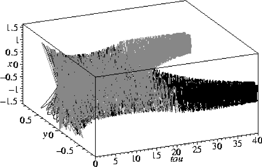
FIG. 1.: An example of highly chaotic dynamics displayed by (84) for two initial conditions given (in the dimensionless variables) by $(x,z,y,w)=(4/\sqrt{6},-10^{-5},0,\pm 10^{-5})$. Time is scaled as $\tau=10^{2}\sqrt{6|m_{\psi}^{2}|}\;t$.

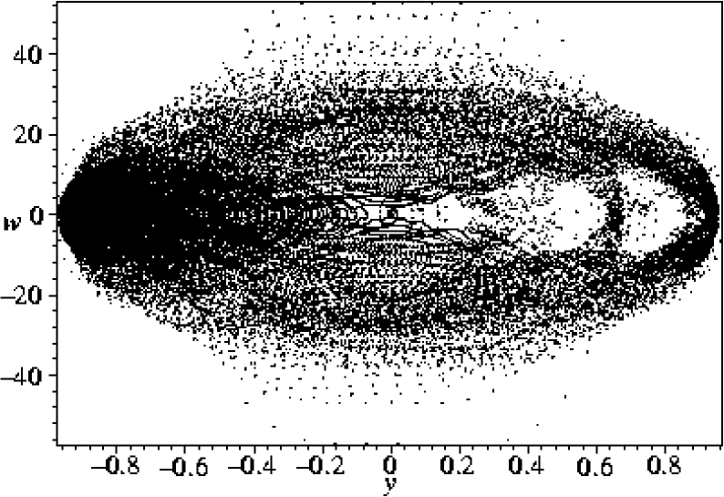
FIG. 2.: The chaotic attractor for one realization of the initial condition $(x,z,y,w)=(4/\sqrt{6},-10^{-5},0,10^{-5})$, for the first dissipation case shown in Table I.

TABLE I.: The fractal dimension $D_{f}$ and the uncertainty exponent $\epsilon$ for increasing dissipation coefficients ($D=4$ is the phase space dimension).

$\{\eta\}=(\eta_{x},\eta_{y},\eta_{xy})$	$D_{f}$	$\epsilon=D-D_{f}$
0.50 $\{\eta\}$	3.96	0.04
0.75 $\{\eta\}$	3.90	0.10
1.00 $\{\eta\}$	3.43	0.57
1.25 $\{\eta\}$	3.23	0.77
1.50 $\{\eta\}$	3.10	0.90

REFERENCES

[1]D. Boyanovsky and H. J. de Vega,
hep-ph/9909372, in the Proceedings of the IV Paris
Cosmology Colloquium (in press).
[2] T. S. Biró, S. G. Matinyan and B. Müller, Chaos and Gauge Field Theory, (World Scientific, Singapore,
1994).
[3] M. Gleiser and R. O. Ramos, Phys. Rev. D50, 2441
(1994); M. Morikawa and M. Sasaki, Phys. Lett. 165B, 59 (1985).
[4] D. Boyanovsky, H. J. de Vega,
R. Holman, D. S-Lee and A. Singh, Phys. Rev. D51,
4419 (1995).
[5] C. Greiner and B. Müller, Phys. Rev. D55,
1026 (1997).
[6] A. Berera, M. Gleiser and R. O. Ramos, Phys. Rev. D58,
123508 (1998).
[7] A. Berera, M. Gleiser and R. O. Ramos, Phys. Rev. Lett.
83, 267 (1999).
[8]E. Calzetta and B. L. Hu, Phys. Rev. D61, 025012 (2000);
Phys. Rev. D40, 656 (1989).
[9]I. D. Lawrie, Phys. Rev. D60, 063510 (1999);
J. Phys. A25, 6493 (1992).
[10] E. Ott, Chaos in Dynamical Systems (Cambridge
University Press, Cambridge 1993).
[11] N. J. Cornish and J. J. Levin, Phys.
Rev. D53, 3022 (1996); Phys. Rev. D55, 7489 (1997).
[12] J. D. Barrow and J. Levin, Phys. Rev. Lett.
80, 656 (1998).
[13]G. Semenoff and N. Weiss, Phys. Rev. D31, 699 (1985);
A. Ringwald, Ann. Phys. 177, 129 (1987); Phys. Rev.
D36, 2598 (1987).
[14]V. Latora and D. Bazeia, Int. J. Mod. Phys. A14,
4967 (1999).
[15]S. Jeon, Phys. Rev. D52, 3591 (1995).
[16]L. G. S. Duarte,
L. A. C. P. da Mota, H. P. de Oliveira, R. O. Ramos and J. E. Skea,
Comp. Phys. Comm. 119, 256 (1999).
[17]
U. Heinz, C. R. Hu, S. Leupold, S. G. Matinian and
B. Müller, Phys. Rev. D55, 2464 (1997);
T. S. Biro and M. H. Thoma, Phys. Rev. D54, 3465 (1996);
T.S. Biro, C. Gong and B. Müller, Phys. Rev. D52,
1260 (1995).
[18]A. D. Linde, Phys. Lett. B259, 38 (1991);
Phys. Rev. D49, 748 (1994).
[19]R. Easther and K. Maeda, Class. Quant. Grav.
16, 1637 (1999).
[20]N. Tetradis, Phys. Rev. D57, 5997 (1998);
C. Panagiotakopoulos and N. Tetradis,
Phys. Rev. D59, 083502 (1999).