Abstract

We review some recent attempts to extract information about the nature of quantum gravity, with and without matter, by quantum field theoretical methods. More specifically, we work within a covariant lattice approach where the individual space-time geometries are constructed from fundamental simplicial building blocks, and the path integral over geometries is approximated by summing over a class of piece-wise linear geometries. This method of “dynamical triangulations” is very powerful in 2d, where the regularized theory can be solved explicitly, and gives us more insights into the quantum nature of 2d space-time than continuum methods are presently able to provide. It also allows us to establish an explicit relation between the Lorentzian- and Euclidean-signature quantum theories. Analogous regularized gravitational models can be set up in higher dimensions. Some analytic tools exist to study their state sums, but, unlike in 2d, no complete analytic solutions have yet been constructed. However, a great advantage of our approach is the fact that it is well-suited for numerical simulations. In the second part of this review we describe the relevant Monte Carlo techniques, as well as some of the physical results that have been obtained from the simulations of Euclidean gravity. We also explain why the Lorentzian version of dynamical triangulations is a promising candidate for a non-perturbative theory of quantum gravity.

1 Introduction

There is at present no satisfactory theory of four-dimensional quantum gravity. This is partly related to the conceptual questions that arise when dealing with fluctuating geometries without reference to any background metric. Addressing these seems to call for a genuinely non-perturbative formulation of quantum gravity. The need for a non-perturbative approach persists in formulations where gravity appears embedded into a larger theory, such as string or M-theory. Although there have been attempts to identify non-perturbative structures within these unified theories (see [1, 2] and many successive papers), they so far seem to have raised as many questions as they have been able to answer. In these lectures we will review an alternative non-perturbative approach to quantum gravity. It is more conservative in spirit, in that it does not conjecture the existence of any radically new physical principles or symmetries. This so-called “dynamical triangulations” approach can be formulated entirely within the framework of ordinary quantum field theory, while taking into account that the governing symmetry principle is reparametrization- (diffeomorphism-) invariance.

Our ansatz can be made in any dimension, and has been solved analytically in two space-time dimensions. In higher dimensions one so far has to rely largely on numerical simulations, and up to now only the case of Euclidean signature has been studied in detail. Although gravity in two dimensions has no genuine dynamical degrees of freedom, it does provide a testing ground for addressing some of the conceptual problems of quantum gravity explicitly, for example, how to define a notion of reparametrization-invariant length in a fluctuating geometry or how to define correlation functions without reference to a background geometry. In 2d Euclidean gravity, a number of questions can be answered by continuum functional methods (within Liouville quantum field theory), but some of the most interesting problems involving geodesic distances can only be addressed in the non-perturbative setting of dynamical triangulations. The fact that in this latter approach quantum gravity is obtained as the scaling limit of a lattice theory shows that, contrary to common belief, discrete methods can be used also for reparametrization-invariant theories, as long as the discretization takes place directly on the space of geometries (that is, on the space of metrics modulo diffeomorphisms).

Another point that has been analyzed in the two-dimensional model is the analytic continuation between geometries of Lorentzian and Euclidean signature. Canonical quantization attempts of (Lorentzian) gravity usually take as their starting point globally hyperbolic manifolds equipped with a non-degenerate Lorentzian metric (which gives rise to a causal structure). However, it is a priori unclear to what extent these essentially classical structures should be preserved in the quantum theory. For example, in a covariant path-integral approach it is not obvious that a causality constraint should be imposed on each individual space-time configuration contributing to the amplitude. This idea was first advocated by Teitelboim [14], and more recently in [15, 16]. One argument in its favour is that it seems hard to imagine how any notion of causality could emerge in the full quantum theory unless it had been imposed in some form on the individual histories in the first place.

Two-dimensional quantum gravity is an ideal testing ground for such ideas, since it can be solved explicitly. We will show that by restricting the state sum to discrete geometries with a causal structure one obtains a theory of quantum gravity with the following features [11, 12].

• The expectation values of reparametrization-invariant space-time distances have canonical dimensions. In other words, in spite of strong fluctuations in the geometry, there is still a sense in which the quantum space-time is two-dimensional.

• When matter with conformal charge $c\leq 1$ is coupled to this Lorentzian quantum gravity theory, both property (1) and the properties of the conformal field theory (critical exponents etc.) remain unchanged.

There is an alternative way of arriving at the same theory, namely, by starting from the geometric configurations of the 2d Euclidean gravity theory, and removing its “baby universes” in a systematic manner. (The proliferation of these branching structures is responsible for most of the fractal and geometric properties of the Euclidean theory.) In this way one creates a many-to-1 correspondence between Euclidean and Lorentzian geometries. Lorentzian 2d quantum gravity appears in this construction as a “renormalized” version of the Euclidean quantum theory [17].

Loosening the requirement of causality for the individual space-time histories, one may allow for changes in the topology of the spatial (constant-time) slices as a function of time, without changing the overall topology of space-time. This is of course tantamount to reintroducing geometries with baby universes. We will show below that once this process is permitted, it will totally dominate the structure of space-time. The resulting theory (which is equivalent to Euclidean Liouville quantum gravity) has the following features.

• The expectation values of geodesic space-time distances have anomalous dimensions, and the intrinsic Hausdorff dimension of quantum space-time is four, and not two [18, 19].

• When matter with conformal charge $c\leq 1$ is coupled to this Euclidean quantum gravity theory, both the fractal properties of the gravitational sector and the critical exponents of the conformal field theory are changed.

We therefore may say that the interaction between gravity and matter is weak in the Lorentzian 2d gravity model, at least as long as $c\leq 1$. Allowing for baby-universe creation leads to a strong coupling between matter and gravity: the fractal properties of space-time become a function of the matter content and in turn the back-reaction of the fluctuating geometry changes the critical properties of the matter. The coupling of Ising models to 2d gravity provides a particularly clear geometric illustration of the role played by the baby universes [20].

If one transcends the so-called $c=1$ barrier, even Lorentzian gravity exhibits a strong gravity-matter interaction, leading to a change in the fractal properties of space-time [13]. In the Euclidean case (i.e. including baby universes), it has been known for a long time that beyond $c=1$ the space-time disintegrates completely into fractals. These so-called branched polymers can be viewed as trees of baby universes of cut-off size. However, this is not what happens in the Lorentzian case. One does observe a phase transition for $c>1$ (to be precise, the transition must take place somewhere in the interval $1<c<4$ [13, 21, 22]), but the new geometry is less pathological than the branched polymers. In particular, the critical matter exponents retain their Onsager values.

Many of the results quoted above for $c>1$ have been obtained by Monte Carlo simulations. Numerical methods have been very successful in the study of discretized quantum gravity. Moreover, in two-dimensional quantum gravity there has been a fruitful interaction between theory and “experiment”. Non-rigorous calculations have been verified or falsified by numerical “experiments”, and “observations” have inspired theoretical progress. In the Lorentzian case, visualizations of the computer-generated space-time geometries have been useful in understanding the influence of matter on geometry [23].

In higher dimensions, only partial results have been obtained by analytical methods. These include asymptotic estimates for the partition functions of dynamically triangulated Euclidean gravity in 3d and 4d [24, 25], and qualitative descriptions of the extreme branched-polymer and crumpled phases [25, 26, 27]. However, as already mentioned, our regularized quantum gravity models can readily be studied by means of computer simulations. In a first step, one determines the phase diagram of the discretized theory, in order to locate potential critical points where a continuum limit can be obtained. One can then use standard finite-size tools to study the scaling of various observables. This method has been very successful and has enabled us to study both the fractal properties of space-time, and the critical exponents of matter coupled to fluctuating geometries.

The rest of this paper is organized as follows. In Section 2.1 we describe and solve the simplest discretized Lorentzian model of 2d gravity, using a “Lorentzian” version of the method of dynamical triangulations. In Section 2.2, the corresponding continuum limit is obtained, while in Section 3 we demonstrate how the inclusion of baby universes changes the structure of quantum space-time. A non-perturbative definition of Euclidean quantum gravity for arbitrary dimension $d$ by means of dynamical triangulations is given in Section 4, where we also discuss the inclusion of matter fields. Section 5 outlines the principles for numerical simulations of the model, with special emphasis on 2d gravity. In Subsection 5.2, we describe various possibilities of defining notions of (fractal) “dimensionality” in the framework of Euclidean quantum gravity. We discuss why these “observables” are particularly well-suited for use in numerical calculations. Subsection 5.3 provides the interpretation of the numerical results obtained in 2d Euclidean quantum gravity. Section 6 describes the numerical approach to higher-dimensional Euclidean quantum gravity. Finally, in Section 7, we outline the future perspectives for both Euclidean and Lorentzian lattice gravity.

2 Lorentzian gravity in 2d

2.1 The discrete model

In order to solve two-dimensional quantum gravity in a path-integral formulation, one has to “count” geometries. Since for a fixed space-time topology the gravitational action consists only of the cosmological term, all geometries of a fixed space-time volume contribute with the same weight. In the simplest model of two-dimensional gravity, no spatial topology changes are allowed either. For simplicity, we choose the spatial slices (at constant “time”) to be circles, so that the overall topology of space-time is of the form $S^{1}\times[0,1]$ (for other spatial boundary conditions, see [28]). This mimicks the situation in classical gravity, where one usually works with globally hyperbolic space-times [29]. We will use a natural class of triangulations of the cylinder $S^{1}\times[0,1]$, to which we will assign edge lengths (i.e. a discretized metric) in such a way that each two-dimensional geometry carries a discrete causal structure. Our simplicial space-times will have a preferred foliation into a discrete set of circular slices, consisting only of space-like edges. The foliation parameter $t$ can be interpreted as a discrete version of “proper time”. The main task of our dynamical-triangulations approach is to count the geometries in this class, that is, to perform the state sum in the regularized context, and then attempt to take a continuum limit.

The geometry of each spatial slice is uniquely characterized by the length assigned to it. In the discretized version, the length $L$ will be “quantized” in units of a lattice spacing $a$, i.e. $L=l\cdot a$ where $l$ is an integer. A slice will thus be defined by $l$ vertices and $l$ links connecting them. To obtain a 2d geometry, we will evolve this spatial loop in discrete steps. This leads to a preferred notion of (discrete) “time” $t$, where each loop represents a slice of constant $t$. The propagation from time-slice $t$ to time-slice $t+1$ is governed by the following rule: each vertex $i$ at time $t$ is connected to $k_{i}$ vertices at time $t+1$, $k_{i}\geq 1$, by links which are assigned squared edge lengths $-a^{2}$. The $k_{i}$ vertices, $k_{i}>1$, at time-slice $t+1$ will be connected by $k_{i}-1$ consecutive space-like links, thus forming $k_{i}-1$ triangles. Finally the right boundary vertex in the set of $k_{i}$ vertices will be identified with the left boundary vertex of the set of $k_{i+1}$ vertices. In this way we get a total of $\sum_{i=1}^{l}(k_{i}-1)$ vertices (and also links) at time-slice $t+1$ and the two spatial slices are connected by $\sum_{i=1}^{l}k_{i}\equiv l_{t}+l_{t+1}$ triangles (see Fig. 1).

Figure 1.  : The propagation of a spatial slice from step $t$ to step $t+1$. The ends of the strip should be joined to form a band with topology $S^{1}\times[0,1]$.

The elementary building blocks of a geometry are therefore triangles with one space- and two time-like edges. We define them to be flat in the interior. A consistent way of assigning interior angles to such Minkowskian triangles is described in [30]. The angle between two time-like edges is $\gamma_{tt}=-\arccos\frac{3}{2}$, and between a space- and a time-like edge $\gamma_{st}=\frac{\pi}{2}+\frac{1}{2}\arccos\frac{3}{2}$, summing up to $\gamma_{tt}+2\gamma_{st}=\pi$. The sum over all angles around a vertex with $j$ incoming and $k$ outgoing time-like edges (by definition $j,k\geq 1$) is given by $2\pi+(4-j-k)\arccos\frac{3}{2}$. The regular triangulation of flat Minkowski space corresponds to $j=k=2$ at all vertices. The volume of a single triangle is given by $\frac{\sqrt{5}}{4}a^{2}$.

One may view these geometries as a subclass of all possible triangulations that allow for the introduction of a causal structure. Namely, if we think of all time-like links as being future-directed, a vertex $v^{\prime}$ lies in the future of a vertex $v$ iff there is an oriented sequence of time-like links leading from $v$ to $v^{\prime}$. Two arbitrary vertices may or may not be causally related in this way.

In quantum gravity we are instructed to sum over all geometries connecting, say, two spatial boundaries of length $L_{1}$ and $L_{2}$, with the weight of each geometry $g$ given by

$$\mbox{e}^{iS[g]},~{}~{}~{}~{}~{}S[g]=\Lambda\int\!\!\sqrt{-\det g}~{}~{}~{}(\mbox{in 2d}),$$ (1)

where $\Lambda$ is the cosmological constant. In our discretized model the boundaries will be characterized by integers $l_{1}$ and $l_{2}$, the number of vertices or links at the two boundaries. The path-integral amplitude for the propagation from geometry $l_{1}$ to $l_{2}$ will be the sum over all interpolating surfaces of the kind described above, with a weight given by the discretized version of (1). Let us call the corresponding amplitude $G^{(1)}_{\lambda}(l_{1},l_{2})$. We thus have

$$G_{\lambda}^{(1)}(l_{1},l_{2}) = \sum_{t=1}^{\infty}G_{\lambda}^{(1)}(l_{1},l_{2};t),$$ (2)

$$G_{\lambda}^{(1)}(l_{1},l_{2};t) = \sum_{l=1}^{\infty}G_{\lambda}^{(1)}(l_{1},l;1)\;l\;G_{\lambda}^{(1)}(l,l_{2},t-1),$$ (3)

$$G_{\lambda}^{(1)}(l_{1},l_{2};1) = \frac{1}{l_{1}}\sum_{\{k_{1},\dots,k_{l_{1}}\}}\mbox{e}^{i\lambda a^{2}\sum_{i=1}^{l_{1}}k_{i}},$$ (4)

where $\lambda$ denotes the bare cosmological constant (we have absorbed the finite triangle volume factor), and where $t$ denotes the total number of time-slices connecting $l_{1}$ and $l_{2}$.

From a combinatorial point of view it is convenient to mark a vertex on the entrance loop in order to get rid of the factors $l$ and $1/l$ in (3) and (4), that is,

$$G_{\lambda}(l_{1},l_{2};t)\equiv l_{1}G_{\lambda}^{(1)}(l_{1},l_{2};t)$$ (5)

(the unmarking of a point may be thought of as the factoring out by (discrete) spatial diffeomorphisms). Note that $G_{\lambda}(l_{1},l_{2};1)$ plays the role of a transfer matrix, satisfying

$$G_{\lambda}(l_{1},l_{2};t_{1}+t_{2}) = \sum_{l}G_{\lambda}(l_{1},l;t_{1})\;G_{\lambda}(l,l_{2};t_{2})$$ (6)

$$G_{\lambda}(l_{1},l_{2};t+1) = \sum_{l}G_{\lambda}(l_{1},l;1)\;G_{\lambda}(l,l_{2};t).$$ (7)

Knowing $G_{\lambda}(l_{1},l_{2};1)$ allows us to find $G_{\lambda}(l_{1},l_{2};t)$ by iterating (7) $t$ times. This program is conveniently carried out by introducing the generating function for the numbers $G_{\lambda}(l_{1},l_{2};t)$,

$$G_{\lambda}(x,y;t)\equiv\sum_{k,l}x^{k}\,y^{l}\;G_{\lambda}(k,l;t),$$ (8)

which we can use to rewrite (6) as

$$G_{\lambda}(x,y;t_{1}+t_{2})=\oint\frac{dz}{2\pi i\,z}\;G_{\lambda}(x,z^{-1};t_{1})G_{\lambda}(z,y;t_{2}),$$ (9)

where the contour should be chosen to include the singularities in the complex $z$–plane of $G_{\lambda}(x,z^{-1};t_{1})$ but not those of $G_{\lambda}(z,y;t_{2})$.

One can either view the introduction of $G_{\lambda}(x,y;t)$ as a purely technical device or take $x$ and $y$ as boundary cosmological constants,

$$x=\mbox{e}^{i\lambda_{i}a},~{}~{}~{}~{}y=\mbox{e}^{i\lambda_{o}a},$$ (10)

such that $x^{k}=\mbox{e}^{i\lambda_{i}a\,k}$ becomes a boundary cosmological term, and similarly for $y^{l}=\mbox{e}^{i\lambda_{o}a\,l}$. Let us for notational convenience define

$$g=\mbox{e}^{i\lambda a^{2}}$$ (11)

(not to be confused with the symbol for the continuum metric). For the technical purpose of counting we view $x,y$ and $g$ as variables in the complex plane. In general the function

$$G(x,y;g;t)\equiv G_{\lambda}(x,y;t)$$ (12)

will be analytic in a neighbourhood of $(x,y,g)=(0,0,0)$.

From the definitions (4) and (5) it follows by standard techniques of generating functions that we may associate a factor $g$ with each triangle, a factor $x$ with each vertex on the entrance loop and a factor $y$ with each vertex on the exit loop, leading to

$$G(x,y;g;1)=\sum_{k=0}^{\infty}\left(gx\sum_{l=0}^{\infty}(gy)^{l}\right)^{k}-\sum_{k=0}^{\infty}(gx)^{k}=\frac{g^{2}xy}{(1-gx)(1-gx-gy)}.$$ (13)

Formula (13) is simply a book-keeping device for all possible ways of evolving from an entrance loop of any length in one step to an exit loop of any length. The subtraction of the term $1/(1-gx)$ has been performed to exclude the degenerate cases where either the entrance or the exit loop is of length zero.

From (13) and eq. (9), with $t_{1}=1$, we obtain

$$G(x,y;g;t)=\frac{gx}{1-gx}\;G(\frac{g}{1-gx},y;g;t-1).$$ (14)

This equation can be iterated and the solution written as

$$G(x,y;g;t)=F_{1}^{2}(x)F_{2}^{2}(x)\cdots F_{t-1}^{2}(x)\frac{g^{2}xy}{[1-gF_{t-1}(x)][1-gF_{t-1}(x)-gy]},$$ (15)

where $F_{t}(x)$ is defined iteratively by

$$F_{t}(x)=\frac{g}{1-gF_{t-1}(x)},~{}~{}~{}F_{0}(x)=x.$$ (16)

Let $F$ denote the fixed point of this iterative equation. By standard techniques one readily obtains

$$F_{t}(x)=F\ \frac{1-xF+F^{2t-1}(x-F)}{1-xF+F^{2t+1}(x-F)},~{}~{}~{}~{}F=\frac{1-\sqrt{1-4g^{2}}}{2g}.$$ (17)

Inserting (17) in eq. (15), we can write

$$G(x,y;g,t)=\frac{F^{2t}(1-F^{2})^{2}\;xy}{(A_{t}-B_{t}x)(A_{t}-B_{t}(x+y)+C_{t}xy)}$$ (18)

$$\hskip 8.5359pt=\frac{F^{2t}(1-F^{2})^{2}\;xy}{\Big{[}(1\!\!-\!xF)\!-\!F^{2t+1}(F\!\!-\!x)\Big{]}\Big{[}(1\!\!-\!xF)(1\!\!-\!yF)\!-\!F^{2t}(F\!\!-\!x)(F\!\!-\!y)\Big{]}},~{}~{}~{}$$ (19)

where the time-dependent coefficients are given by

$$A_{t}=1-F^{2t+2},~{}~{}~{}B_{t}=F(1-F^{2t}),~{}~{}~{}C_{t}=F^{2}(1-F^{2t-2}).$$ (20)

The combined region of convergence to the expansion in powers $g^{k}x^{l}y^{m}$, valid for all $t$ is

$$|g|<\frac{1}{2},~{}~{}~{}~{}|x|<1,~{}~{}~{}~{}|y|<1.$$ (21)

2.2 The continuum limit

The path integral formalism we are using here is very similar to the one used to represent the free particle as a sum over paths. Also there one performs a summation over geometric objects (the paths), and the path integral itself serves as the propagator. From the particle case it is known that the bare mass undergoes an additive renormalization (even for the free particle), and that the bare propagator is subject to a wave-function renormalization (see [8] for a review). The same is true in two-dimensional Euclidean gravity, treated in the formalism of dynamical triangulations [8]. The coupling constants with positive mass dimension, i.e. the cosmological constant and the boundary cosmological constants, undergo an additive renormalization, while the partition function itself (i.e. the Hartle-Hawking-like wave function) undergoes a multiplicative wave-function renormalization. We therefore expect the bare coupling constants $\lambda,\lambda_{i}$ and $\lambda_{0}$ to behave as

$$\lambda=\frac{C_{\lambda}}{a^{2}}+\tilde{\Lambda},~{}~{}~{}~{}\lambda_{i}=\frac{C_{\lambda_{i}}}{a}+\tilde{X},~{}~{}~{}\lambda_{o}=\frac{C_{\lambda_{o}}}{a}+\tilde{Y},$$ (22)

where $\tilde{\Lambda},\tilde{X},\tilde{Y}$ denote the renormalized cosmological and boundary cosmological constants. If we introduce the notation

$$g_{c}=\mbox{e}^{iC_{\lambda}},~{}~{}~{}~{}x_{c}=\mbox{e}^{iC_{\lambda_{i}}},~{}~{}~{}~{}y_{c}=\mbox{e}^{iC_{\lambda_{o}}},$$ (23)

for critical values of the coupling constants, it follows from (10) and (11) that

$$g=g_{c}\,\mbox{e}^{ia^{2}{\tilde{\Lambda}}},~{}~{}~{}~{}x=x_{c}\,\mbox{e}^{ia{\tilde{X}}},~{}~{}~{}~{}y=y_{c}\,\mbox{e}^{ia{\tilde{Y}}}.$$ (24)

The wave-function renormalization will appear as a multiplicative cut-off dependent factor in front of the bare “Green’s function” $G(x,y;g;t)$,

$$G_{\tilde{\Lambda}}({\tilde{X}},{\tilde{Y}};T)=\lim_{a\to 0}a^{\eta}G(x,y;g;t),$$ (25)

where $T=a\,t$, and where the critical exponent $\eta$ should be chosen so that the right-hand side of eq. (25) exists. In general this will only be possible for particular choices of $g_{c},x_{c}$ and $y_{c}$ in (25).

The basic relation (6) can survive the limit (25) only if $\eta=1$, since we have assumed that the boundary lengths $L_{1}$ and $L_{2}$ have canonical dimensions and satisfy $L_{i}=a\,l_{i}$.

A closer analysis reveals that only at $g_{c}=1/2$ one can obtain a sensible continuum limit. It corresponds to a purely imaginary bare cosmological constant $\lambda_{c}:=C_{\lambda}/a^{2}=-i\ln 2/a^{2}$. If we want to approach this point from the region in the complex $g$-plane where $G(x,y;g;t)$ converges it is natural to choose the renormalized coupling ${\tilde{\Lambda}}$ imaginary as well, ${\tilde{\Lambda}}=i\Lambda$, i.e.

$$\lambda=i\ \frac{\ln\frac{1}{2}}{a^{2}}+i\Lambda.$$ (26)

One obtains a well-defined scaling limit (corresponding to $\Lambda\in{\rm I\!R}$) by letting $\lambda\to\lambda_{c}$ along the imaginary axis. The Lorentzian form for the continuum propagator is obtained by an analytic continuation $\Lambda\to-i\Lambda$ in the renormalized coupling of the resulting Euclidean expressions.

At this stage it may seem that we are surreptitiously reverting to a fully Euclidean model. We could of course equivalently have conducted the entire discussion up to this point in the “Euclidean sector”, by omitting the factor of $-i$ in the exponential (1) of the action, choosing $\lambda$ positive real and taking all edge lengths equal to 1. However, from a purely Euclidean point of view there would not have been any reason for restricting the state sum to a subclass of geometries admitting a causal structure. The associated preferred notion of a discrete “time” allows us to define an “analytic continuation in time”. Because of the simple form of the action in two dimensions, the rotation

$$\int dx\ dt\sqrt{-\det g_{lor}}\to i\int dx\ dt_{eu}\sqrt{\det g_{eu}}$$ (27)

to Euclidean metrics in our model is equivalent to the analytic continuation of the cosmological constant $\Lambda$.

From (18) or (19) it follows that we can only get macroscopic loops in the limit $a\to 0$ if we simultaneously take $x,y\to 1$. (For $g_{c}=-1/2$, one needs to take $x,y\to-1$. The continuum expressions one obtains are identical to those for $g_{c}=1/2$.) Again the critical points correspond to purely imaginary bare boundary cosmological coupling constants. We will allow for such imaginary couplings and thus approach the critical point $\lambda_{i}=\lambda_{o}=0$ from the region of convergence of $G(x,y;g;t)$, i.e. via real, positive $X,Y$ where

$$\lambda_{i}=iXa,~{}~{}~{}~{}\lambda_{o}=iYa.$$ (28)

Again $X$ and $Y$ have an obvious interpretation as positive boundary cosmological constants in a Euclidean theory, which may be analytically continued to imaginary values to reach the Lorentzian sector.

Summarizing, we have

$$g=\frac{1}{2}\mbox{e}^{-\Lambda a^{2}}\to\frac{1}{2}(1-\Lambda a^{2}),~{}~{}~{}(\mbox{i.e.}~{}~{}F=1-a\sqrt{\Lambda})$$ (29)

as well as

$$x=\mbox{e}^{-Xa}\to 1-aX,~{}~{}~{}~{}~{}~{}y=\mbox{e}^{-aY}\to 1-aY,$$ (30)

where the arrows $\to$ in (29) and (30) should be viewed as analytic coupling constant redefinitions of $\Lambda,X$ and $Y$, which we have performed to get rid of factors of 1/2 etc. in the formulas below. With the definitions (29) and (30) it is straightforward to perform the continuum limit of $G(x,y;g;t)$ as $(x,y,g)\to(x_{c},y_{c},g_{c})=(1,1,1/2)$, yielding

$$G_{\Lambda}(X,Y;T)=\frac{4\Lambda\ \mbox{e}^{-2\sqrt{\Lambda}T}}{(\sqrt{\Lambda}+X)+\mbox{e}^{-2\sqrt{\Lambda}T}(\sqrt{\Lambda}-X)}$$

$$\hskip 14.22636pt\times\,\frac{1}{(\sqrt{\Lambda}+X)(\sqrt{\Lambda}+Y)-\mbox{e}^{-2\sqrt{\Lambda}T}(\sqrt{\Lambda}-X)(\sqrt{\Lambda}-Y)}.$$ (31)

For $T\to\infty$ one finds

$$G_{\Lambda}(X,Y;T)\buildrel T\rightarrow\infty\over{\longrightarrow}\frac{4\Lambda\;\mbox{e}^{-2\sqrt{\Lambda}T}}{(X+\sqrt{\Lambda})^{2}(Y+\sqrt{\Lambda})},$$ (32)

while the limit for $T\to 0$ is

$$G_{\Lambda}(X,Y;T\!=\!0)=\frac{1}{X+Y},$$ (33)

in accordance with the expectation that

$$G_{\Lambda}(L_{1},L_{2};T\!=\!0)=\delta(L_{1}-L_{2}).$$ (34)

The general expression for $G_{\Lambda}(L_{1},L_{2};T)$ can be computed as the inverse Laplace transform of formula (31), yielding

$$G_{\Lambda}(L_{1},L_{2};T)=\frac{\mbox{e}^{-[\coth\sqrt{\Lambda}T]\sqrt{\Lambda}(L_{1}+L_{2})}}{\sinh\sqrt{\Lambda}T}\;\frac{\sqrt{\Lambda L_{1}L_{2}}}{L_{2}}\;\;I_{1}\left(\frac{2\sqrt{\Lambda L_{1}L_{2}}}{\sinh\sqrt{\Lambda}T}\right),$$ (35)

where $I_{1}(x)$ is a modified Bessel function of the first kind. The asymmetry between $L_{1}$ and $L_{2}$ arises because the entrance loop has a marked point, whereas the exit loop has not. The amplitude with both loops marked is obtained by multiplying with $L_{2}$, while the amplitude with no marked loops is obtained after dividing (35) by $L_{1}$. Quite remarkably, our highly non-trivial expression (35) agrees with the loop propagator obtained from a bona-fide continuum calculation in proper-time gauge of pure 2d gravity by Nakayama [31].

The basic result (31) for $G_{\Lambda}(X,Y;T)$ can be derived by taking the continuum limit of the recursion relation (14). By inserting (29) and (30) in eq. (14) and expanding to first order in the lattice spacing $a$ we obtain

$$\frac{\partial}{\partial T}G_{\Lambda}(X,Y;T)+\frac{\partial}{\partial X}\Bigl{[}(X^{2}-\Lambda)G_{\Lambda}(X,Y;T)\Bigr{]}=0.$$ (36)

This is a standard first-order partial differential equation which should be solved with the boundary condition (33) at $T=0$, since this expresses the natural condition (34) on $G_{\Lambda}(L_{1},L_{2})$. The solution is thus

$$G_{\Lambda}(X,Y;T)=\frac{\bar{X}^{2}(T;X)-\Lambda}{X^{2}-\Lambda}\;\frac{1}{\bar{X}(T;X)+Y},$$ (37)

where $\bar{X}(T;X)$ is the solution to the characteristic equation

$$\frac{d\bar{X}}{dT}=-(\bar{X}^{2}-\Lambda),~{}~{}~{}~{}\bar{X}(T=0)=X.$$ (38)

It is readily seen that the solution is indeed given by (31) since we obtain

$$\bar{X}(T)=\sqrt{\Lambda}\;\frac{(\sqrt{\Lambda}+X)-\mbox{e}^{-2\sqrt{\Lambda}T}(\sqrt{\Lambda}-X)}{(\sqrt{\Lambda}+X)+\mbox{e}^{-2\sqrt{\Lambda}T}(\sqrt{\Lambda}-X)}.$$ (39)

If we interpret the propagator $G_{\Lambda}(L_{1},L_{2};T)$ as the matrix element between two boundary states of a Hamiltonian evolution in “time” $T$,

$$G_{\Lambda}(L_{1},L_{2};T)=\langle L_{1}|\mbox{e}^{-\hat{H}T}|L_{2}\rangle$$ (40)

we can, after an inverse Laplace transformation, read off the functional form of the Hamiltonian operator $\hat{H}$ from (36),

$$\hat{H}(L,\frac{\partial}{\partial L})=-L\frac{\partial^{2}}{\partial L^{2}}+L\Lambda.$$ (41)

The corresponding Hamiltonian for the propagator of unmarked loops is given by

$$\hat{H}_{u}(L,\frac{\partial}{\partial L})=-L\frac{\partial^{2}}{\partial L^{2}}-2\frac{\partial}{\partial L}+\Lambda L.$$ (42)

The Hamiltonian (42) is Hermitian with respect to the natural measure $L\,\mbox{d}L$, which has its origin in the basic completeness relation (3) for the transfer matrix with unmarked entrance and exit loops. If one wants to construct a unitary evolution with respect to the “time”-parameter $T$ appearing in the transfer-matrix approach, one can simply exponentiate $(i\hat{H}T)$.

However, we should point out that there is an alternative to the analytic continuation $T\to-iT$ if one wants to relate the Euclidean and Lorentzian sectors of the theory. The combination $\sqrt{\Lambda}T$ appearing as an argument in (35) arises in taking the continuum limit of powers of the form $F^{t}$ in expressions like (18), (19), where $F$ is defined in (17). There are two aspects to a possible analytic continuation of $F^{t}$. The power $t$ in $F^{t}$ should clearly not be continued, since it is simply an integer counting the number of iterations of the transfer matrix. However, the function $F$ itself does refer to the action, because the dimensionless coupling constant $g=\mbox{e}^{i\lambda a_{t}a_{l}}$ is the action for a single Lorentzian triangle. (For added clarity we have distinguished between the lattice spacings in time- and space-directions, and called them $a_{t}$ and $a_{l}$.) From the expression for $F$ in terms of $g$ in (17), we have $F=1-\sqrt{a_{t}a_{l}\Lambda}$. The analytic continuation of $F$ in time, from Euclidean to Lorentzian time, corresponds to the substitution $a_{t}\to-i\ a_{t}$ under the square-root sign, and thus becomes equivalent to the continuation $\Lambda\to-i\Lambda$ in the cosmological constant, as already remarked below eq. (27). The subtleties associated with the analytic continuation in the “time”-parameter $T$ appearing in a transfer-matrix formulation of quantum gravity were first discussed in [32, 33] in the context of a square-root action formulation. Similar difficulties will also be present in higher-dimensional gravity, where the analytic continuation from Euclidean metrics to Lorentzian metrics cannot be absorbed by a continuation in $\Lambda$ alone. To conclude, it is not obvious how to choose the correct analytic continuation back to Lorentzian signature, once the continuum limit has been taken. The continuation $T\to-iT$ leads to a unitary theory. For the continuation $\Lambda\to-i\Lambda$, we have not yet found a scalar product which makes the corresponding evolution operator unitary.

3 Topology changes and Euclidean quantum gravity

3.1 Baby universe creation

In our non-perturbative regularization of 2d quantum gravity we have so far not included the possibility of topology changes of space. We will now show that if one allows for spatial topology changes, one is led in an essentially unambiguous manner to a different theory of two-dimensional quantum gravity, where space-time is much more fractal, and which agrees with Euclidean 2d quantum gravity as defined by Euclidean dynamical triangulations or Liouville theory.

By a topology change of space in our Lorentzian setting we have in mind the following: a baby universe may branch off at some time $T$ and develop in the future, where it will eventually disappear in the vacuum, but it is not allowed to rejoin the “parent” universe and thus change the overall topology of the two-dimensional manifold. This is a restriction we impose to be able to compare with the analogous calculation in usual 2d Euclidean quantum gravity.

It is well known that such a branching leads to additional complications, compared with the Euclidean situation, in the sense that, in general, no continuum Lorentzian metrics which are smooth and non-degenerate everywhere can be defined on such space-times (see, for example, [34] and references therein). These considerations do not affect the cosmological term in the action, but lead potentially to contributions from the Einstein-Hilbert term at the singular points where a branching or pinching occurs.

We have so far ignored the curvature term in the action since it gives merely a constant contribution in the absence of topology change. We will continue to do so in the slightly generalized setting just introduced. The continuum results of [34] suggest that the contributions from the two singular points associated with each branching of a baby universe (one at the branching point and one at the tip of the baby universe where it contracts to a point) cancel in the action. The physical geometry of these configurations may seem slightly contrived, but they may well be important in the quantum theory of gravity and deserve further study. However, for the moment our main motivation for introducing them is to make contact with the usual non-perturbative Euclidean path-integral results.

We will use the rest of this section to demonstrate the following: once we allow for spatial topology changes,

• this process completely dominates and changes the critical behaviour of the discretized theory, and

• the disc amplitude $W_{\Lambda}(L)$ (the Hartle-Hawking wave function) is uniquely determined, almost without any calculations.

Our starting point will be the discretized model introduced in Sec. 2.1. In this model we do not directly have a disc amplitude like the Hartle-Hawking wave functional. However, as discussed at the beginning of this section, the degeneracy of the metric at a point in the interior of the disc is always compensated (in the sense of complex contributions to the action) by the degeneracy of the metric at the point where the baby universe branched off. We can thus define the disc amplitude in Lorentzian gravity as

$$w^{(b)}(x,g):=\sum_{t}G^{(b)}(x,l_{2}\!=\!1;g;t)=G^{(b)}(x,l_{2}\!=\!1;g),$$ (43)

and the continuum version as

$$W^{(b)}_{\Lambda}(X)=\int\mbox{d}T\;G^{(b)}_{\Lambda}(X,L_{2}\!=\!0;T)=G^{(b)}_{\Lambda}(X,L_{2}\!=\!0)$$ (44)

where the superscript ^(b) indicates the “bare” Lorentzian model without spatial topology changes. It follows that

$$w^{(b)}(x,g)\to a^{-1}W^{(b)}_{\Lambda}(X).$$ (45)

There are a number of ways to implement the creation of baby universes, some more natural than others, but they all agree in the continuum limit, as will be clear from the general arguments provided below. Here we discuss only the simplest way of implementing such a change. This is shown in Fig. 2: stepping forward from $t$ to $t+1$ from a loop of length $l_{1}$ we create a baby universe of length $l<l_{1}$ by pinching it off non-locally from the main branch.

Figure 2.  : A “baby universe” created by a global pinching.

Accounting for the new possibilities of evolution in each step according to fig. 2, the new and old transfer matrices are related by

$$G_{\lambda}(l_{1},l_{2};1)=G_{\lambda}^{(b)}(l_{1},l_{2};1)+\sum_{l=1}^{l_{1}-1}l_{1}w(l_{1}\!-\!l,g)\,G_{\lambda}^{(b)}(l,l_{2};1).$$ (46)

The factor $l_{1}$ in the sum comes from the fact that the “pinching” shown in fig. 2 can take place at any of the $l_{1}$ vertices. As before, the new transfer matrix leads to new amplitudes $G_{\lambda}(l_{1},l_{2};t)$, satisfying

$$G_{\lambda}(l_{1},l_{2};t_{1}+t_{2})=\sum_{l}G_{\lambda}(l_{1},l;t_{1})G_{\lambda}(l,l_{2};t_{2}),$$ (47)

and in particular

$$G_{\lambda}(l_{1},l_{2};t)=\sum_{l}G_{\lambda}(l_{1},l;1)\;G_{\lambda}(l,l_{2};t\!-\!1).$$ (48)

Performing a (discrete) Laplace transformation of eq. (48) leads to

$${G(x,y;g;t)=}~{}~{}~{}~{}~{}~{}~{}~{}~{}~{}~{}~{}~{}~{}~{}~{}~{}~{}~{}~{}~{}~{}~{}~{}~{}~{}~{}~{}~{}~{}~{}~{}~{}~{}~{}~{}~{}~{}~{}~{}~{}~{}~{}~{}~{}~{}~{}~{}~{}~{}~{}~{}~{}~{}~{}~{}~{}~{}~{}~{}~{}~{}~{}~{}~{}~{}~{}~{}~{}~{}~{}~{}~{}~{}~{}~{}~{}$$

$$\oint\frac{dz}{2\pi i\,z}\;\left[G_{\lambda}^{(b)}(x,z^{-1};1)\!+\!x\frac{\partial}{\partial x}\Bigl{(}w(x;g)G_{\lambda}^{(b)}(x,z^{-1};1)\Bigr{)}\right]G(z,y;g;t\!-\!1),$$

or, using the explicit form of the transfer matrix $G_{\lambda}^{(b)}(x,z;1)$, formula (13),

$$G(x,y;g;t)=\Bigl{[}1+x\frac{\partial w(x,g)}{\partial x}+xw(x,g)\frac{\partial}{\partial x}\Bigr{]}\,\frac{gx}{1-gx}\,G\Bigl{(}\frac{g}{1\!-\!gx},y;g;t\!-\!1\Bigr{)}.$$ (50)

At this point neither the disc amplitude $w(x,g)$ nor $G(x,y;g;t)$ are known. We will now show that they are uniquely determined if we assume that the boundary length scales canonically with the lattice spacing, $L=a\,l$, implying a renormalized boundary cosmological constant $X$ with the dimension of mass, $x=x_{c}(1-aX)$. In addition we assume that the dimension of the renormalized cosmological constant $\Lambda$ is canonical too, $g=g_{c}(1-\frac{1}{2}\Lambda a^{2})$. Somewhat related arguments have been presented in different settings in [35, 36].

It follows from relation (47) that we need

$$G_{\lambda}(l_{1},l_{2},t)\buildrel a\rightarrow 0\over{\longrightarrow}a\,G_{\Lambda}(L_{1},L_{2};T).$$ (51)

It is important for the following discussion that $G_{\lambda}(l_{1},l_{2};t)$ cannot contain a non-scaling part since from first principles (sub-additivity) it has to decay exponentially in $t$. By a Laplace transformation, using $x=x_{c}(1-aX)$ in the scaling limit, we thus conclude that

$$G_{\lambda}(x,l_{2},t)\buildrel a\rightarrow 0\over{\longrightarrow}G_{\Lambda}(X,L_{2},T),$$ (52)

and further, by a Laplace transformation in $L_{2}$,

$$G_{\lambda}(x,y;t)\buildrel a\rightarrow 0\over{\longrightarrow}a^{-1}G_{\Lambda}(X,Y;T).$$ (53)

We will now show that the scaling of $w(x,g)$ is quite restricted too. The starting point is a combinatorial identity which the disc amplitude has to satisfy. The arguments are valid both for the disc amplitude in Euclidean quantum gravity and the disc amplitude we have introduced for our model in (43). We will assume the general scaling

$$w(x,g)=w_{ns}(x,g)+a^{\eta}W_{\Lambda}(X)+\mbox{less singular terms}$$ (54)

for the disc amplitude. In the case $\eta<0$ the first term is considered absent (or irrelevant). However, if $\eta>0$ a term like $w_{ns}$ will generically be present, since any slight redefinition of the coupling constants of the model will produce such a term if it was not there from the beginning.

We will introduce an explicit mark in the bulk of $w(x,g)$ by differentiating with respect to $g$. This leads to the combinatorial identity

$$g\ \frac{\partial w(x,g)}{\partial g}=\sum_{t}\sum_{l}G(x,l;g;t)\,l\,w(l,g),$$ (55)

or, after the usual Laplace transform,

$$g\ \frac{\partial w(x,g)}{\partial g}=\sum_{t}\oint\frac{dz}{2\pi i\,z}\;G(x,z^{-1};g;t)\;\frac{\partial w(z,g)}{\partial z}.$$ (56)

The situation is illustrated in Fig. 3. A given mark has a distance $t$ ($T$ in the continuum) to the entrance loop. In the figure we have drawn all points which have the same distance to the entrance loop and which form a connected loop. In the bare model these are all the points at distance $t$. In the case where baby universes are allowed (which we have not included in the figure), there can be many disconnected loops at the same distance.

Figure 3.  : Marking a vertex in the bulk of $W_{\Lambda}(X)$. The mark has a distance $T$ from the boundary loop, which itself has one marked vertex.

Let us assume a general scaling

$$T=a^{\varepsilon}t,~{}~{}~{}~{}~{}\varepsilon>0,$$ (57)

for the time variable $T$ in the continuum limit. Above we saw that the bare model without baby universe creation corresponded to $\varepsilon=1$. With the generalization (57) we account for the fact that by allowing for baby universes we have introduced an explicit asymmetry between the time- and space-directions.

Inserting (54) and (57) into eq. (56) we obtain

$$\frac{\partial w_{ns}}{\partial g}-2a^{\eta-2}\frac{\partial W_{\Lambda}(X)}{\partial\Lambda}=$$

$$\hskip 17.07182pt\frac{1}{a^{\varepsilon}}\int\mbox{d}T\int dZ\;G_{\Lambda}(X,-Z;T)\bigg{[}\frac{\partial w_{ns}}{\partial z}-a^{\eta-1}\frac{1}{z_{c}}\frac{\partial W_{\Lambda}(Z)}{\partial Z}\bigg{]},$$ (58)

where $(x,g)=(x_{c},g_{c})$ in the non-singular part.

From eq. (58) and the requirement $\epsilon>0$ it follows that the only consistent choices for $\eta$ are

• ${\eta<\ }$0,   i.e.

  $$a^{\eta-2}\frac{\partial W_{\Lambda}(X)}{\partial\Lambda}=\frac{a^{\eta-1}}{2a^{\varepsilon}}\int\mbox{d}T\int dZ\;G_{\Lambda}(X,-Z;T)\;\frac{1}{z_{c}}\frac{\partial W_{\Lambda}(Z)}{\partial Z},$$ (59)

  in which case we get $\varepsilon=1$; and

• 1${\ <\eta<\ }$2. Here formula (58) splits into the two equations

  $$-a^{\eta-2}\frac{\partial W_{\Lambda}(X)}{\partial\Lambda}=\frac{1}{2a^{\varepsilon}}\,\frac{\partial w_{ns}}{\partial z}\bigg{|}_{z=x_{c}}\;\int\mbox{d}T\int dZ\;G_{\Lambda}(X,-Z;T),$$ (60)

  and

  $$\frac{\partial w_{ns}}{\partial g}\bigg{|}_{g=g_{c}}=-\frac{a^{\eta-1}}{a^{\varepsilon}}\int\mbox{d}T\int dZ\;G_{\Lambda}(X,-Z;T)\;\frac{1}{z_{c}}\frac{\partial W_{\Lambda}(Z)}{\partial Z}.$$ (61)

  We are led to the conclusion that $\varepsilon=1/2$ and $\eta=3/2$, which are precisely the values found in Euclidean 2d gravity. Let us further remark that eq. (60) in this case becomes

  $$-\frac{\partial W_{\Lambda}(X)}{\partial\Lambda}=\mbox{const.}\;G_{\Lambda}(X,L_{2}=0),$$ (62)

  which differs from (44) by a derivative with respect to the cosmological constant. We will explain the reason for this difference below. Finally, eq. (61) becomes

  $$\int\mbox{d}T\int dZ\;G_{\Lambda}(X,-Z;T)\;\frac{\partial W_{\Lambda}(Z)}{\partial Z}=\mbox{const.},$$ (63)

  which will be satisfied automatically if $\eta=3/2$ and $\varepsilon=1/2$, as we will show below.

We will now analyze a possible scaling limit of (50), assuming the canonical scaling $x=x_{c}(1-aX)$ and $g=g_{c}(1-\frac{1}{2}\Lambda a^{2})$. In order that the equation have a scaling limit at all, $x_{c},\,g_{c}$ and $w_{ns}(x_{c},g_{c})$ must satisfy two relations which can be determined straightforwardly from (50). The remaining continuum equation reads

$$a^{\varepsilon}\frac{\partial}{\partial T}\,G_{\Lambda}(X,Y;T) = -a\,\frac{\partial}{\partial X}\Bigl{[}(X^{2}-\Lambda)G_{\Lambda}(X,Y;T)\Bigr{]}$$ (64)

$$-a^{\eta-1}\frac{\partial}{\partial X}\Bigl{[}W_{\Lambda}(X)G_{\Lambda}(X,Y;T)\Bigr{]}.$$

The first term on the right-hand side of eq. (64) is precisely the one we have already encountered in our original model, while the second term is due to the creation of baby universes. Clearly the case $\eta<0$ (in fact $\eta\leq 1$) is inconsistent with the presence of the second term, i.e. the creation of baby universes. However, since $\eta<2$, the last term on the right-hand side of (64) will always dominate over the first term. Once we allow for the creation of baby universes, this process will completely dominate the continuum limit. In addition we get $\varepsilon=\eta-1$, in agreement with (61). It follows that $\eta>1$ and we conclude that $\varepsilon=1/2,\eta=3/2$ are the only possible scaling exponents if we allow for the creation of baby universes. These are precisely the scaling exponents obtained from two-dimensional Euclidean gravity in terms of dynamical triangulations, as we have already remarked. The topology changes of space have induced an anomalous dimension for $T$. If the second term on the right-hand side of (64) had been absent, this would have led to $\varepsilon=1$, and the time $T$ scaling in the same way as the spatial length $L$.

In summary, in the case $(\eta,\varepsilon)=(3/2,1/2)$ eq. (64) leads to the continuum equation

$$\frac{\partial}{\partial T}\,G_{\Lambda}(X,Y;T)=-\frac{\partial}{\partial X}\Bigl{[}W_{\Lambda}(X)G_{\Lambda}(X,Y;T)\Bigr{]},$$ (65)

which, combined with eq. (62), determines the continuum disc amplitude $W_{\Lambda}(X)$. Integrating (65) with respect to $T$ and using that $G_{\Lambda}(L_{1},L_{2};T\!=\!0)=\delta(L_{1}\!-\!L_{2})$, i.e.

$$G_{\Lambda}(X,L_{2}\!=\!0;T\!=\!0)=1,$$ (66)

we obtain

$$-1=\frac{\partial}{\partial X}\bigg{[}W_{\Lambda}(X)\frac{\partial}{\partial\Lambda}W_{\Lambda}(X)\bigg{]}.$$ (67)

Since $W_{\Lambda}(X)$ has length dimension –3/2, i.e. $W_{\Lambda}^{2}(X)=X^{3}F(\sqrt{\Lambda}/X)$, the general solution must be of the form

$$W_{\Lambda}(X)=\sqrt{-2\Lambda X+b^{2}X^{3}+c^{2}\Lambda^{3/2}}.$$ (68)

From the very origin of $W_{\Lambda}(X)$ as the Laplace transform of a disc amplitude $W_{\Lambda}(L)$ which is bounded, it follows that $W_{\Lambda}(X)$ has no singularities or cuts for $\mbox{Re}\,X>0$. This requirement fixes the constants $b,c$ in (68) such that

$$W_{\Lambda}(X)=b\Big{(}X-\frac{\sqrt{2}}{b\,\sqrt{3}}\,\sqrt{\Lambda}\Big{)}\sqrt{X+\frac{2\sqrt{2}}{b\,\sqrt{3}}\sqrt{\Lambda}},$$ (69)

where the constant $b$ is determined by the model-dependent constant in (62). This expression for the disc amplitude agrees after a rescaling of the cosmological constant with the amplitude $W^{(eu)}_{\Lambda}(X)$ from 2d Euclidean quantum gravity,

$$W_{\Lambda}(X)=(X-\frac{1}{2}\sqrt{\Lambda})\sqrt{X+\sqrt{\Lambda}}.$$ (70)

With $W_{\Lambda}(X)$ substituted into (65), the resulting equation is familiar from the usual theory of 2d Euclidean quantum gravity, where it has been derived in various ways [18, 35, 36], with $T$ playing the role of geodesic distance between the initial and final loop.

Before showing that the anomalous scaling of the proper time – once baby universes are allowed – leads to an intrinsic fractal space-time dimension of four (rather than two), let us comment on the difference between the equations for the amplitudes (59)-(61) for $(\eta,\varepsilon)=(-1,1)$ and $(\eta,\varepsilon)=(3/2,1/2)$ respectively. In the first case there are no baby universes and eq. (59) entails that only macroscopic loops at a distance $T$ from the entrance loop are important (as illustrated in Fig. 3). On the other hand, the term $\partial W_{\Lambda}(Z)/\partial Z$ which describes the presence of these macroscopic loops is absent in eq. (60). This is consistent with eq. (62), which shows explicitly that the length of the upper loop in Fig. 3 remains at the cut-off scale, and therefore can never become macroscopic. It is also consistent with the abundance of baby universes, since at any point in space-time the probability for creating a little “tip” of cut-off size will dominate. At the same time, the right-hand side of eq. (59), that is, eq. (63), will play no role when $1<\eta<2$, being simply equal to a constant. This latter property is satisfied automatically, as can be seen by using an equation analogous to (65) for the exit instead of the entrance loop. Thus eq. (63) becomes proportional to

$$\int_{0}^{\infty}\mbox{d}T\frac{\partial}{\partial T}\;G(X,L_{2}\!=\!0;T)=\mbox{const.},$$ (71)

proving our previous assertion.

3.2 The fractal dimension of Euclidean 2d gravity

If we allow for baby universe creation, the fractal structure of space-time is determined by (65) and (70), where $T$ is the time separating the entrance and exit loops. As already mentioned, these are exactly the equations governing Euclidean quantum gravity, if one replaces $T$ by the geodesic distance between the two loops.

One can solve eq. (65) in the same way as its Lorentzian analogue (36) was solved by (37)-(39). We have

$$G_{\Lambda}(X,Y;T)=\frac{W_{\Lambda}(\bar{X}(T;X))}{W_{\Lambda}(X)}\;\frac{1}{\bar{X}(T;X)+Y},$$ (72)

where $\bar{X}(T;X)$ is the solution to the characteristic equation

$$\frac{d\bar{X}}{dT}=-W_{\Lambda}(\bar{X}),~{}~{}~{}~{}~{}\bar{X}(T=0)=X.$$ (73)

This equation can be solved in terms of elementary functions. In particular, one finds

$$\bar{X}(T;X=\infty)\propto\sqrt{\Lambda}\,\coth^{2}\Big{(}\alpha\Lambda^{1/4}T\Big{)},~{}~{}~{}~{}\alpha=\frac{1}{2}\sqrt{3/2}.$$ (74)

We may now define a two-point function by contracting the entrance loop to a point and closing the exit loop by the disc amplitude. This is shown in Fig. 3, except that now the entrance loop must be contracted. The two-point function $G_{\Lambda}(T)$ in Euclidean gravity can be interpreted as the (unnormalized) average over all geometries with two marked points which are separated by a geodesic distance $T$. At the discretized level it is defined by an equation analogous to (55), but without summing over $t$,

$$G(t;g)=\sum_{l}G(l_{1},l;g;t)\;l\;w(l,g).$$ (75)

As in eq. (58), the continuum limit will be dominated by the non-scaling part of $w(l;g)$, i.e. by small $l$, and the continuum two-point function is simply given by

$$G_{\Lambda}(T)\sim G_{\Lambda}(L_{1}\!=\!0,L_{2}\!=\!0;T).$$ (76)

Using (72) and the Laplace transforms of $G_{\Lambda}$ and $W_{\Lambda}$ we obtain

$$G_{\Lambda}(T)=\oint\frac{\mbox{d}X}{2\pi i}\oint\frac{\mbox{d}Y}{2\pi i}\;\frac{W_{\Lambda}(\bar{X}(T;X))}{W_{\Lambda}(X)}\;\frac{1}{\bar{X}(T;X)+Y}.$$ (77)

With the help of the characteristic equation (73) this leads to

$$G_{\Lambda}(T)\sim\frac{\mbox{d}}{\mbox{d}T}\oint\frac{\mbox{d}X}{2\pi i}\;\frac{\bar{X}(T;X)}{W_{\Lambda}(X)}.$$ (78)

The contour of integration can be deformed to infinity and we obtain from (74) that

$$G_{\Lambda}(T)\sim\Lambda^{3/4}\;\frac{\cosh{\alpha\Lambda^{1/4}T}}{\sinh^{3}\alpha\Lambda^{1/4}T}.$$ (79)

This two-point function may be viewed as the partition function for universes with two marked points separated by a geodesic distance $T$. Since we wanted to solve Euclidean gravity, this is our final result. Given (79), we can calculate the average space-time volume of such a universe,

$$\left\langle V\right\rangle_{T}=T^{4}F\Big{(}\Lambda^{1/4}T\Big{)},~{}~{}~{}~{}F(0)>0.$$ (80)

The function $F$ is again expressible in terms of elementary functions and one finds

$$\left\langle V\right\rangle_{T}\approx T^{4}~{}~{}~{}{\rm for}~{}~{}~{}T<1/\Lambda^{1/4}.$$ (81)

This formula shows that the intrinsic fractal dimension of 2d Euclidean quantum space-time is four, whereas a similar derivation in the case of Lorentzian gravity yields [11]

$$\left\langle V\right\rangle_{T}\approx T^{2}~{}~{}~{}{\rm for}~{}~{}~{}~{}T<1/\Lambda^{1/2}.$$ (82)

The discrepancy in dimension can be explained purely in terms of the baby universe structure: since at each point of the two-dimensional Lorentzian surface a baby universe can branch off, the resulting fractal Euclidean space-time has twice the intrinsic dimension.

4 Euclidean quantum gravity

4.1 Some generalities

In the last section we arrived at the 2d Euclidean gravity theory through an “extension” of the Lorentzian model. Euclidean quantum gravity can of course be defined independently, as the quantization of classical gravity on the space of all Riemannian metrics (of positive definite signature) instead of the space of (indefinite-signature) Lorentzian metrics. In two dimensions, Euclidean gravity has a well-defined continuum path-integral formulation. Choosing a conformal gauge-fixing leads to the so-called Liouville gravity. Certain aspects of this theory can be solved by a bootstrap approach. In higher dimensions the path-integral approach to Euclidean quantum gravity is problematic, since the Einstein-Hilbert action is unbounded from below. There are various ways of tackling this problem: analytically continuing the unstable modes, adding stabilizing higher-derivative terms to the action, or defining the theory non-perturbatively via a lattice regularization, such that the action is bounded for any finite lattice volume.

One example of the latter is the dynamical-triangulations approach, which has the added bonus of being exactly soluble by combinatorial methods in two dimensions. Its continuum limit agrees with continuum Liouville quantum gravity, wherever the two formulations can be compared. We are in fact in the unusual situation that the lattice approach can address and answer more questions than the continuum methods. We will not review the combinatorial approach here since the results (for pure gravity) were already obtained in Section 3, starting from Lorentzian gravity. For a detailed description we refer to [8], chapter 4. The generalization of this Euclidean lattice path integral to higher dimensions is straightforward and shares two virtues with the 2d case: calculating the partition function for gravity is again turned into a combinatorial problem, and the model is well-suited for numerical simulations. We have by now a good qualitative understanding of the phase structure of Euclidean dynamically-triangulated gravity in $d=3,4$, although complete analytical solutions of the discretized models are still missing. However, the combinatorial nature of the partition function gives us some hope that progress can be made also in these cases.

4.2 Dynamical triangulations

This lattice approach shares many elements with lattice regularizations of ordinary quantum field theory. The main difference lies in the fact that the geometric degrees of freedom become dynamical and the lattices are therefore no longer part of the inert background structure. The geometric quantum fluctuations must be taken properly into account when building discretized models of matter interacting with quantum gravity. The field-theoretical, non-perturbative Euclidean path integral of such a theory takes the general form

$$Z[G,\Lambda,\{\beta_{i}\}]=\int{\cal D}[g_{\mu\nu}]{\cal D}\phi_{i}\ e^{-S_{matter}[g_{\mu\nu},\phi_{i};\{\beta_{i}\}]-S_{EH}[g_{\mu\nu};G,\Lambda]},$$ (83)

where the integration is over equivalence classes of metrics $[g_{\mu\nu}]$ and matter fields $\phi_{i}$. The action contains a matter part $S_{matter}$, depending on a set of matter couplings $\{\beta_{i}\}$, and a purely geometric part, given by the Einstein-Hilbert action with a cosmological term,

$$S_{EH}[g_{\mu\nu};G,\Lambda]=\frac{1}{16\pi G}\int d^{d}x\ \sqrt{\det g}\,(2\Lambda-R).$$ (84)

In (83) we have omitted possible boundary terms. Except in $d=2$, expressions of the kind (83) have remained formal, due to the absence of a suitable diffeomorphism-invariant integration measure. The lattice formulation is an attempt to remedy this situation, by using an intermediate regularization of the non-perturbative path integral (83) (see [37, 8] for reviews). Defining a discrete regularization consists of several steps:

• a discretization of the individual metric manifolds, together with a definition of discretized geometric “observables”, such as lengths, volumes and (scalar) curvature. These are necessary for obtaining a discretized version of the action, and for analyzing the physical properties of the theory in terms of scaling relations and correlation functions.

• a suitable choice of an integration measure on the space of discretized geometries (i.e. equivalence classes of metrics), such that the discrete path integral converges.

• a discretization of the matter sector, which will be closely related to standard lattice-regularizations in field theory.

Let us now describe the dynamical-triangulations regularization of Euclidean quantum gravity. It consists in replacing the $d$-dimensional Riemannian metric continuum manifold by a simplicial manifold constructed from equilateral $d$-dimensional simplices of (geodesic) edge length $a$. (A simplex is a point in $d=0$, an edge in $d=1$, a triangle in $d=2$, a tetrahedron in $d=3$, etc.) Using Regge’s prescription [38], all quantities can be expressed as functions of the squared edge lengths. For example, the curvature depends on local deficit angles, which in turn are expressible in terms of edge lengths. A simplicial complex is obtained by gluing together $d$-simplices pairwise along $(d-1)$-dimensional faces (which are themselves $(d-1)$-simplices). Since, unlike in Regge calculus, our edge lengths are not variable, all $d$-simplices have the same size, and the total volume of the simplicial complex is simply proportional to the number $N_{d}$ of such cells. Each $d$-simplex is built from simplices of lower dimensionality. It contains $d+1$ 0-simplices (vertices), $(d+1)d/2$ 1-simplices (links) etc. A lower-dimensional subsimplex is in general shared by a number of $d$-simplices, called the order of the subsimplex. A simplicial complex is a simplicial manifold if the neighbourhood of any $p$-simplex ($p<d$) has the topology of a $(d-p-1)$-dimensional sphere. Physically the manifold requirement may be viewed as a regularity condition at the cut-off scale, which will be convenient to use in our construction. The numbers $N_{k}$ of (sub-)simplices of dimension $k\leq d$ are not independent, but (due to the regularity requirement) must satisfy a set of so-called Dehn-Sommerville relations, namely,

$$N_{i}=\sum_{k=1}^{d}(-1)^{k+d}\left(\begin{array}[]{c}k+1\\ i+1\end{array}\right)N_{k},$$ (85)

together with the Euler constraint

$$\sum_{k=0}^{d}(-1)^{k}N_{k}=\chi.$$ (86)

For fixed Euler number $\chi$ and $d=2$, all $N_{k}$ can be expressed as functions of the single variable $N_{2}$, say. For $d=3,4$, two of the $N_{k}$ are independent.

A triangulation $T$ together with an assignment of geodesic edge lengths and flat simplex interiors may be viewed as a piecewise linear manifold, and provides an explicit coordinate-independent representation of a metric manifold. In this way each triangulation corresponds to a unique equivalence class of metrics (albeit of piecewise-linear, and not of differentiable type).

When it comes to numerical simulations, it is often convenient to assign a label to each vertex. From the list of vertex labels for all $d$-simplices the whole manifold can be reconstructed. Since the labels themselves have no physical meaning, the labelling introduces a redundancy. Invariance under permutations of the labels may loosely be regarded as a discrete analogue of the diffeomorphism invariance of a differentiable manifold. Also the lower-dimensional subsimplices are characterized by their vertex labels. Moreover, the regularity requirement implies that we cannot have two different (sub-)simplices with the same set of vertex labels. For each triangulation $T$ with $N_{0}$ vertices the number of different labellings equals $N_{0}!/C(T)$, where $C(T)$ is the order of the automorphism group of $T$. We can therefore distinguish between labelled triangulations $\tilde{T}$ and abstract unlabelled triangulations $T$. As mentioned above, different $T$’s (with fixed topology) correspond to different equivalence classes of piecewise linear metrics assigned to the underlying manifold, and allow us to work directly with a reparameterization-invariant set of geometries.

Since the simplices are flat on the inside, curvature is located (distributionally) at simplices of lower dimension. Circulating around a $(d-2)$-dimensional simplex, the contributing angles will in general not add up to $2\pi$. The resulting deficit angle depends on the number of simplices meeting at the subsimplex. We conclude that the curvature is concentrated at the $(d-2)$-dimensional subsimplices of the triangulation. The Einstein-Hilbert action for a dynamically triangulated manifold in dimension $d$ assumes the simple form

$$S_{EH}=\kappa_{d}N_{d}-\kappa_{d-2}N_{d-2},$$ (87)

with the two dimensionless coupling constants $\kappa_{d}$ and $\kappa_{d-2}$. As usual in lattice regularizations, the lattice spacing $a$ has disappeared from the formulation and will have to be reintroduced in the scaling limit. We are using the Einstein-Hilbert action because of its simplicity; one could in principle consider also the inclusion of higher-order curvature terms.

With each simplicial lattice described above one can associate a dual lattice, whose vertices are located at the centres of the simplices of the original lattice. In a similar way we can associate to each $p$-simplex a dual object of dimension $d-p$. For example, the dual links connect the centres of neighbouring simplices, and the dual of a $(d-2)$-simplex is a closed loop (a two-dimensional object) whose length is equal to the number of $d$-simplices of the original lattice which share the $(d-2)$-simplex. Since in $d$ dimensions each simplex has $d+1$ neighbours, the dual lattices have the form of graphs of a scalar $\bf{\phi}^{d+1}$-theory (that is, all their vertices are $(d+1)$-valent), but with a local $d$-dimensional topological structure.

The simplicial structures described above possess a natural notion of length for any path connecting two points, since the equivalence class of metrics is uniquely determined. To simplify matters, we will only consider certain sets of discretized paths on the simplicial manifold. The first set is given by paths which run along the links of the original simplicial lattice, and the other by paths running along the links of the dual lattice. In either case we may define a distance between points on the lattice or its dual as the number of edges of the shortest path connecting the two. At first glance these definitions seem different from the standard notion of a geodesic distance, but they all coincide in the scaling limit, up to trivial numerical factors. Numerical tests of this assumption will be discussed below.

4.3 The functional integral

The association of triangulations with equivalence classes of metrics motivates the use of the discrete sum over $d$-dimensional triangulations as a discretized analogue of the diffeomorphism-invariant integration measure in (83),

$$\int{\cal D}[g_{\mu\nu}]\to\sum_{T}{1\over C(T)},$$ (88)

where the sum is taken over unlabelled simplicial manifolds. The need for including the symmetry factor $C(T)$ becomes apparent when one rewrites the right-hand side of (88) as a sum over labelled triangulations $\tilde{T}$,

$$\sum_{T}{1\over C(T)}\to\sum_{\tilde{T}}{1\over N_{0}(\tilde{T})!}.$$ (89)

In order that a discretized path integral with this choice of measure lead to a theory with a well-defined thermodynamic limit, the number of triangulations with fixed volume $N_{d}$ should grow at most exponentially with $N_{d}$ as $N_{d}\to\infty$. This is not the case unless we fix the space-time topology (usually to that of a sphere S^d); otherwise the growth is factorial. This property has been proven for $d=2$ and arbitrary topology [39] and for simply connected manifolds in $d=3,4$ [24, 25].

It is worthwhile pointing out that the simple choices (87) for the action and (88) for the measure lead to a partition function of the form

$$Z(g_{d},g_{d-2})=\sum_{T}\frac{1}{C(T)}\;g^{N_{d}(T)}_{d}\,g_{d-2}^{N_{d-2}(T)},$$ (90)

where $g_{d}=-\log\kappa_{d}$ and $g_{d-2}=\log\kappa_{d-2}$. Eq. (90) shows that the partition function is the generating function for the number of triangulations (of fixed topology) with given numbers $N_{d}$ and $N_{d-2}$ of $d$- and $(d-2)$-simplices. We thus reach the surprising conclusion that even in dimension $d>2$, quantum gravity can be formulated as a (relatively simple) counting problem.

4.4 Inclusion of matter fields

The discretization of matter fields coupled to dynamical triangulations is achieved by standard lattice field-theoretical methods. The simplest types of matter fields one can study are either scalar fields or (Potts) spin fields, carrying a discrete space-time label. One may also combine several fields of this type. The matter fields can be located at the vertices of the triangulation or at the centres of the $d$-simplices (that is, at the dual vertices). The interactions are typically of the form of nearest-neighbour interactions, where the “nearest neighbours” are the vertices that are one link length (or one dual link length) away from the original vertex. We expect these two formulations to become equivalent in the scaling limit. Some typical examples of matter actions are

$$S_{I}={\beta\over 2}\sum_{\{ij\}}(\delta_{\sigma_{i}\sigma_{j}}-1),$$ (91)

where the $\sigma_{i}$ are a set of Potts spins, or the Gaussian action

$$S_{g}=\sum_{\{ij\}}(\phi_{i}-\phi_{j})^{2}$$ (92)

for a massless scalar field $\phi$. Note that we did not need to include a coupling constant in front of the action (92). The massless scalar field can always be rescaled by a factor, which can then be absorbed by a redefinition of the coupling constants of the geometric sector. The coupling of Ising spins (Potts spins $\sigma_{i}$ with $i=1,2$) and Gaussian fields to the 2d Lorentzian gravity model proceeds in a manner identical to (91) and (92).

In higher dimensions we will also consider the coupling to gauge fields. As usual these are associated with the one-dimensional edges of the triangulation, and there are again two alternative formulations, depending on whether the links or the dual links are used. The gauge field action is more complicated and we postpone its discussion to Section 6. The inclusion of fermionic degrees of freedom on a random manifold remains an open problem, particularly in higher dimensions. It requires the definition of a spin connection on a simplicial manifold (c.f. [40]). The problem was solved in $d=2$ [41]. In this case one can prove that a system of Wilson fermions on a triangulated manifold can be “bosonized” and represented as a system of Ising spins on the manifold [42, 41].

The discretized path-integral measure contains also a sum over matter fields. In the case of spin variables, the sum is simply taken over all possible spin configurations. For continuous fields like the scalar fields above, one may consider non-trivial integration measures which introduce an additional coupling to geometry. This possibility does not exist in field theories on fixed, regular lattices, where such a dependence is always trivial. It leads to some subtleties in the case of gauge fields, as we will discuss later.

The simplest and most extensively studied example of a dynamically triangulated theory is that of Euclidean gravity on a two-sphere. The fundamental building blocks in this case are equilateral triangles (2-simplices). Triangles are glued together pairwise along edges (1-simplices), and each triangle has exactly three neighbours. The dual lattice is thus equivalent to a planar $\bf{\phi}^{3}$-diagram. The curvature is localized at the vertices (0-simplices) which in general are shared by many triangles, each contributing $\pi/3$ to the total angle around the vertex. The regularity requirement introduced above prohibits configurations where a vertex is its own neighbour or where two vertices are connected by more than one link (in other words, closed loops of link length one or two are forbidden).

The Lorentzian gravity model introduced in Section 2.1 may be viewed as a restricted version of the dynamically triangulated Euclidean model, since the triangulations contributing to the Lorentzian state sum constitute a subset of those appearing in the Euclidean system defined above. Recall also our construction of Euclidean from Lorentzian gravity in Section 3.1, by allowing for additional baby-universe branching. Again the set of all such geometries is a subset of all 2d simplicial manifolds, but both continuum theories coincide. What is at work in this latter case is “universality”, which ensures that the continuum limit is to a large extent independent of the short-distance details characterizing the class of triangulations we sum over. The universality properties of Euclidean 2d quantum gravity are well studied. For example, one may relax the manifold regularity condition to obtain a much larger class of simplicial complexes, whose continuum limit is still Euclidean quantum gravity. Only drastic modifications, like the suppression of baby universes, can move the system to a different universality class with a different critical behaviour and therefore a different continuum limit. Also around the fixed point leading to Lorentzian 2d gravity one finds an independence of short-distance details. Universality with respect to a change of fundamental building blocks and the inclusion of higher curvature has been demonstrated in [28]. It is also encountered in a recently developped procedure for obtaining Lorentzian from Euclidean quantum gravity by removing baby universes [17]. There one ends up with a generalized class of triangulations (compared to the original Lorentzian model), but the continuum limit is still the same.

5 Numerical setup

5.1 Monte Carlo method and ergodic moves

Even in two dimensions, there are a number of issues of the matter-coupled theory that presently can only be addressed by numerical methods. Lorentzian gravity coupled to Ising spins has not yet been solved analytically. In matter-coupled Euclidean 2d quantum gravity, analytical considerations have not yet led to a determination of the fractal dimension of space-time (there are various suggestions leading to different answers), nor do we know what happens beyond the infamous $c=1$ barrier, where analytical calculations break down. In higher dimensions, we do not even have analytical solutions of the pure-gravity models. In all of these situations, numerical simulations of the systems come in handy. They can answer specific questions and lead to unexpected results which in turn can inspire further analytical work.

Numerical simulations of simplicial gravity have been the subject of a number of reviews (see [9, 43] for annual updates and [44] for more information on the computer codes used in the programs). Here we will only sketch the methods and use the simplest case of 2d Euclidean gravity as an illustration. Most of what we will have to say carries over to 2d Lorentzian gravity with only minor modifications.

As explained in the previous section, the discretized theory can be described by the partition function

$$Z=\sum_{\tilde{T}}\frac{1}{N_{0}(\tilde{T})!}e^{-S_{EH}(\tilde{T})}\sum_{\phi_{i}}e^{-S_{matter}(\phi_{i})},$$ (93)

where $S_{EH}$ is the discretized Einstein-Hilbert action (87), and the first sum is taken over all labelled triangulations of fixed spherical topology. For $d=2$, the geometric part of the action simplifies and takes the form

$$S_{EH}=\mu N_{2},$$ (94)

up to an additive constant proportional to the Euler number $\chi$, with $\mu=(\kappa_{2}-\kappa_{0})/2$. In numerical simulations, it is simpler to use the labelled instead of the unlabelled triangulations. The partition function (93) is the analogue of the grand canonical partition function in statistical mechanics. The cosmological constant $\kappa_{d}$ plays the role of a thermodynamic potential for the number of simplices. For general $d$, we may rewrite (93) as

$$Z=\sum_{N_{d}}e^{-\kappa_{d}N_{d}}Z_{N_{d}},$$ (95)

where $Z_{N_{d}}$ can be interpreted as the partition function at fixed volume. A gravity-matter configuration $C$ is uniquely specified by a geometry in the form of a labelled triangulation and by the values of all matter field variables. Each configuration enters the statistical sum with a probability proportional to $e^{-S(C)}$, where $S(C)=S_{EH}+S_{matter}$. As usual in statistical mechanics, physical information can be obtained by measuring the averages of various operators in this ensemble. The fact that each configuration has a real positive weight makes it possible to study the system (93) by Monte Carlo methods. The goal is to construct a numerical “generator” which produces configurations $C$ with a probability $P(C)\sim e^{-S(C)}$.

Except for very few cases, where a direct generation of all configurations is possible (e.g. for a conformal charge $c=-2$ in 2d), the standard way of obtaining such a generator is by means of a stochastic process (a Markov chain), which can be regarded as a random walk in configuration space. Since the random walk takes place on a computer, each step corresponds to the real time needed to perform such an operation. The stochastic process is defined by a function $W(C\to C^{\prime})\geq 0$, giving the probability for a transition from a configuration $C$ to $C^{\prime}$ in one step. Assuming for simplicity that the configuration space is discrete, we have a normalization condition

$$\sum_{C^{\prime}}W(C\to C^{\prime})=1.$$ (96)

In most cases $W(C\to C^{\prime})$ is chosen to vanish outside some “neighbourhood” of $C$. Starting from an initial state $p_{0}(C)$, the system after $n$ steps is characterized by a probability distribution $p_{n}(C)$, where

$$p_{n+1}(C)=\sum_{C^{\prime}}p_{n}(C^{\prime})W(C^{\prime}\to C).$$ (97)

The transition probability $W$ must satisfy two basic requirements,

• ergodicity: any two configurations can be joined by a finite number of steps, and

• detailed balance: the condition

  $$P(C)W(C\to C^{\prime})=P(C^{\prime})W(C^{\prime}\to C),$$ (98)

  relating $W(C\to C^{\prime})$ to $W(C^{\prime}\to C)$.

It follows from (98) that $W(C\to C^{\prime})$ and $W(C^{\prime}\to C)$ are either both zero or both non-zero in which case they satisfy

$$\frac{W(C\to C^{\prime})}{W(C^{\prime}\to C)}=\frac{P(C^{\prime})}{P(C)}.$$ (99)

These two requirements guarantee that the stochastic process has a unique asymptotic probability distribution $p_{\infty}(C)\sim P(C)$, which is the only eigenstate of the transition matrix $W$ with eigenvalue 1,

$$\sum_{C^{\prime}}p_{\infty}(C^{\prime})W(C^{\prime}\to C)=p_{\infty}(C).$$ (100)

All other eigenvalues are strictly smaller than 1. This implies that – independent of the initial configuration – the system will reach the asymptotic distribution after infinitely many steps. Note that the asymptotic distribution has the desired probability distribution. The rate at which the system approaches this limiting distribution depends on the other eigenvalues of $W$. The contributions from other eigenstates decay exponentially with the number of steps. The second-largest eigenvalue $\lambda_{1}$ provides us with an estimate of the autocorrelation time $T=-1/\log\lambda_{1}$. When the number $n$ of steps is $\gg T$, we can assume that the distribution is asymptotic. Typically the autocorrelation time behaves like $T\sim f^{\delta}$, where $f$ counts the number of degrees of freedom of the system and $\delta$ is a dynamical exponent, depending on the details of the algorithm.

In a practical implementation the system starts from some configuration $C_{0}$. During the first step, it changes to $C_{1}$ with probability $W(C_{0}\to C_{1})$, or remains at $C_{0}$ if the change is not accepted. After $n\gg T$ steps it reaches a configuration $C_{n}=C^{(1)}$ with a probability proportional to $P(C^{(1)})$. This configuration is the starting point of a new process, during which another sufficiently large number of steps is performed and a new configuration $C^{(2)}$ generated. Repeating this process we create a (finite) set of configurations $\{C^{(1)},\dots,C^{(N)}\}$, where $N$ depends on the computer time we spend on the project. The average of any operator in the ensemble of configurations defined by the probability distribution $P(C)$ is approximated by an average over this finite sample of “typical” configurations.

The requirements listed above by no means define the stochastic process uniquely. We are interested in efficient algorithms which minimize $\delta$, and can produce a large number of independent configurations in the shortest possible time. There is no simple way to guess at the outset whether an algorithm is efficient or not. Each problem must be treated individually and the autocorrelation time measured numerically. There are some general guidelines which one usually follows when creating a new algorithm. As discussed above, the efficiency depends on the choice of the transition probabilities $W(C\to C^{\prime})$. We would like the algorithm to have a high “mobility”, that is, a high probability that a configuration of the system will change at each step. This means that the set $\{C^{\prime}\}$ of configurations which can be reached from a given $C$ should be limited. If it is too large, each transition probability will be small, implying that the configuration will most likely not change. On the other hand, the set {$C^{\prime}$} must be large enough to ensure ergodicity.

The detailed-balance condition (99) implies that if both transitions are to be reasonably probable, we must choose the set {$C^{\prime}$} such that its elements have similar probabilities to that of $C$ (equivalently, have a small action difference $|S(C)-S(C^{\prime})|$). On a fixed lattice, small differences in the action are usually realized by considering at each step only local changes in the field variables, for instance, changing only one variable, while keeping all the others fixed. When a more complicated change is attempted, the action difference is in general large and proportional to the volume of the system. Local changes are not very efficient when the typical fluctuations are long-ranged, as happens close to a continuous phase transition. Creating a Monte Carlo algorithm which is at the same time ergodic and has a reasonably small autocorrelation time even in the critical region is an art.

The first step in constructing an algorithm for simplicial gravity is to define a method of coding the configurations. From a numerical point of view it is natural to work with labelled rather than unlabelled triangulations, because otherwise it is almost impossible to keep track of the (dynamical) connectivity. To code the geometric structure of such a configuration it is in principle sufficient to have a list of the vertex labels of all simplices (of all dimensions) of the triangulation. Two vertices are neighbours if they belong to the same simplex. From this list we can reconstruct the complete geometry of the system. The fact that we have a list of simplices means in practice that we have also assigned labels to the simplices. Two simplices are neighbours if they share a $(d-1)$-simplex or, equivalently, $d$ vertices. In addition, we can make a list of all subsimplices and count their order. The process of reconstruction may still be complicated and it is often useful to keep at each step even more information, in the extreme case the lists of all subsimplices. The more information we keep, the easier it is to reconstruct local properties of the geometry. However, it also means that during geometry updates more data will have to be changed.

The next step consists in constructing the stochastic process described above. In our case this amounts to defining a set of “moves”, which connect configurations with different geometry and matter content. Usually these two changes are performed separately: changes of the matter fields are performed for a fixed geometric configuration, by techniques very similar to those used for fixed lattices. For spin systems there exist highly effective cluster algorithms [45] with very short autocorrelation times. Cluster algorithms are special in that they permit global changes of the spin configurations. For Gaussian fields, no such algorithms exist and the field variables are usually updated sequentially. (There are some methods to shorten their autocorrelation time.) Generally speaking, the autocorrelation times for Gaussian fields are much longer than those for spin systems. It is therefore necessary to repeat the updating of all fields on the manifold several times in order to obtain independent field configurations.

In addition, we must define a set of geometric moves which generate local changes of the geometry, while preserving its underlying topology. Such moves are necessary even in the absence of matter. “Local changes” means that only a small region of the manifold is affected at each step. Again, it is important that the set of moves be ergodic in the space of all possible triangulations. For simplicial manifolds, one possible choice is given by the so-called Alexander moves [46]. In practical applications most algorithms for a $d$-dimensional geometry are based on a finite subset of moves containing $d+1$ operations. We will describe this set of operations in the case of 2d and postpone its generalization to higher $d$ to Section 6.

The first operation is called a flip and involves two neighbouring triangles. The triangles are denoted by their vertex labels, $\{123\}$ and $\{124\}$, and share the link $\{12\}$. It is important that the four labels are all distinct (excluding $\{3\}=\{4\}$, say) and that the vertices $\{3\}$ and $\{4\}$ are not connected by a link. The flip consists in replacing this configuration by the two triangles $\{341\}$ and $\{342\}$. In other words, the link $\{12\}$ is “flipped” to the link $\{34\}$. The restrictions imposed above guarantee that this move does not produce a pathological triangulation. The inverse of the flip operation is again a flip. Note that the flip move takes place entirely inside the link loop $\{1324\}$, whose boundary it leaves unchanged. Since two simplices are replaced by two others, the flip is sometimes called a $(2,2)$-move. A flip can be performed almost everywhere in the manifold, giving rise to a different labelled manifold whose connectivity is changed locally. If matter fields are present at the vertices, one usually assumes that their values are unchanged. The transition weights $W(C\to C^{\prime})$ and $W(C^{\prime}\to C)$ for a flip and its inverse can easily be computed from the detailed-balance condition. We will not be more specific here, since this depends on the details of the geometric coding (in particular, on how links are selected). A flip move leaves the numbers of triangles and vertices unchanged.

The second move adds a new vertex $\{4\}$ inside a triangle $\{123\}$. This move replaces the old triangle by the three triangles $\{124\}$, $\{234\}$ and $\{314\}$, and leaves the manifold outside the “boundary” of $\{123\}$ unaffected. It is also known as a $(1,3)$-move. The new vertex is of order three, since it is shared by three triangles. The third move is the inverse of the $(1,3)$-move. It is a $(3,1)$-move where a vertex of order three is removed, and the three triangles which share it are replaced by a single triangle. The $(1,3)$-move can be performed on each triangle of a manifold, but its inverse needs a vertex of coordination number three. It is obvious that in both cases the configurations before and after the move are two different labelled triangulations. If matter fields are present, a new field must be created at the new vertex generated during a $(1,3)$-move. This must be taken into account when the transition weights are calculated. The three types of moves are depicted in Fig. 4.

Figure 4.  : A set of three moves which is ergodic in the class of two-dimensional triangulations of fixed topology. The first diagram shows the $(3,1)$-move and its inverse. The second diagram shows the $(2,2)$- or flip move. By itself, this move is ergodic in the class of triangulations of fixed volume $N_{2}$ and topology.

The three operations just described leave the manifold topology unchanged. They form an ergodic set, which means that any two simplicial manifolds of the same topology can be related by a finite sequence of moves. In 2d one can construct such a sequence explicitly. The set of ergodic moves is not unique, and alternative sets of local moves have been used in applications. For example, a point-splitting algorithm is described in [8]. The point-splitting move and its inverse (illustrated in Fig. 5) change the volume $N_{2}$ by $\pm 2$. The $(1,3)$- and $(3,1)$-moves are special cases and the $(2,2)$-move can be realized as a sequence of two point-splitting moves.

Figure 5.  : The point-splitting moves constitute an alternative set of ergodic moves.

Our discussion so far suggests that we may set up a numerical simulation by generating configurations according to the probability distribution (93), and use the resulting sample of configurations to measure the quantities of interest. However, this is not really feasible, since the system described by (93) is an open system in the sense that arbitrarily large configurations may be produced by using one of the sets of geodesic moves described above. In practice, we must limit this size because of the obvious memory restrictions of a computer. A simple solution is to generate a set of configurations of fixed volume $N_{2}$, and repeat the experiment for various values of $N_{2}$. This is what one typically does in numerical simulations of field theory. For the case of Euclidean 2d triangulations we are particularly lucky, since the (2,2)-flip move is already by itself ergodic in the space of all triangulations of fixed volume $N_{2}$, considerably simplifying the computer simulations. Unfortunately there is no similar result in higher dimensions; we will describe later the method used in this case. The flip move cannot be used in numerical simulations of the Lorentzian model described in Section 2.1, since it is not compatible with the causal structure. One uses instead a version of the point-splitting move (Fig. 6) to update the geometry (see [12] for details).

Figure 6.  : The move used in the Monte Carlo updating of a 2d Lorentzian geometry.

We conclude this section by describing another type of move which is associated with a large change in matter and geometry (while keeping $\Delta S$ small). It is motivated by the baby-universe structure of Euclidean simplicial gravity. Let us consider a two-dimensional triangulated manifold with the topology of a disc. It is characterized by its volume $n$ and boundary length $l$. For a random geometry these two numbers are not related since for any finite $l$, $n$ can become arbitrarily large. If we have two such discs, of volume $n$ and $N-n$, but with identical boundary lengths, we can identify their boundaries to create a closed simplicial complex of spherical topology and volume $N_{2}=N$. The smaller component is the baby universe and the larger one the parent universe. A typical spherical manifold observed in numerical simulations will contain many structures of this kind, of various sizes and lengths of boundaries, called “necks”. The shortest possible neck has length three, and the associated baby universe will be called a minimal baby universe (minbu). We may also have baby universes characterized by longer (but finite and small) neck sizes.

The existence of baby universes opens a completely new possibility for updating the matter sector of the theory. Note that for a finite boundary length $l$, the interaction between the matter in the baby universe and the parent universe will be of order $l$. Take the example of Ising spins: even if we flip all spins inside the baby universe, the change in the action will only depend on the interactions across the boundary, and not the size $n$ of the baby universe. This is a completely different situation than on a regular lattice where large domains always have large boundaries. We may use this observation to define a matter update which induces a large change in magnetization and has a large acceptance. The efficiency of such an algorithm will depend on the typical baby universe size. One possible algorithm consists in searching the triangulation for a minimal neck and flip all spins inside the associated minbu with probability $W$. The same technique can be applied to massless scalar fields. Here we can perform two operations on the fields in the minbu: change all of their signs and/or add the same constant to all of them.

The existence of minbus can be exploited also in the geometric sector. For example, we may use the following three-step algorithm.

• Locate a minimal neck in the triangulation, and cut open the original spherical manifold along the neck. Both of the resulting discs are of the form of a triangulated sphere with a triangle removed.

• Close off both holes by a single triangle, to obtain two spherical triangulations of volumes $n+1$ and $N-n+1$ (if the original triangulation had volume $N$).

• Remove an arbitrary triangle from each of the two manifolds, and glue the resulting discs along their triangular boundaries.

We must compute the correct probability factors for such a move and eventually also include changes in the matter fields. Based on this idea, an extremely efficient “minbu surgery” algorithm has been constructed, shortening the autocorrelation times by three orders of magnitude [16]. The move does not even require a lot of geometric updating if it is accepted, since the connectivities of the manifold are changed only locally. The minbu surgery usually supplements the local moves described earlier, although in 2d one may construct an algorithm that is based exclusively on the cutting and pasting of baby universes, if one permits also longer neck lengths. (A flip move may be viewed as a particular realization of this, if instead of minbus we consider baby universes with boundaries of length $l=4$.)

5.2 Observables in 2d Euclidean gravity

The Monte Carlo method described above can be used to generate a set of uncorrelated configurations of volume $N_{2}$ which are distributed according to their Boltzmann weights $e^{-S}$. In order to understand the finite-size effects, one needs to perform the simulations at different values of $N_{2}$. The sizes that have been used in numerical simulations to date range from 1000 to 128000 simplices.

In 2d it speeds up the calculations to extend the class of allowed triangulations to include also loops of link length one and two (corresponding to self-energy and tadpole subdiagrams on the dual lattice). Let us denote this extended class by ${\cal T}$ and the corresponding class of labelled triangulations by $\tilde{{\cal T}}$. Although the complexes constructed in this way are no longer simplicial manifolds, we can still keep the notions of global topology, of local neighbourhoods and of a geodesic distance. Likewise, the relations between the numbers $N_{k}$ remain unchanged. In some cases (including pure 2d gravity), models based on this set of geometries can be compared directly with the analytic solutions of corresponding matrix models, where the exclusion of tadpole and self-energy subdiagrams corresponds merely to a finite renormalization of the bare coupling constants. On ${\cal T}$, the numerical simulations become even simpler. For fixed volume, the flip move is still ergodic and also the minbu surgery moves can be generalized. The advantage of using this class of triangulations is a reduction of the finite-size effects, since it turns out that the local restrictions on the connectivity do not affect the scaling properties of the system.

Our next step will be to describe the measurement of suitable “observables” on the ensemble of configurations generated by the Monte Carlo algorithm. The observables most easily obtained are the critical exponents related to the geometry or the matter fields. In two dimensions, one can sometimes obtain such observables analytically, and use them to test the validity of the numerical results. Recall that in 2d we start from the partition function

$$Z=\sum_{\tilde{{\cal T}}}{1\over N_{0}!}\sum_{\phi_{i}}e^{-\mu V-S_{matter}(\phi_{i})}=\sum_{V}e^{-\mu V}Z_{V},$$ (101)

where $Z_{V}$ is the partition function at fixed volume. If the central charge of matter is $c<1$, it can be shown analytically that $Z_{V}$ behaves like

$$Z_{V}\sim e^{\mu_{0}V}V^{\gamma_{str}-3}(1+{\cal O}(1/V))$$ (102)

for large $V$ and spherical topology. The subleading power contains the critical exponent $\gamma_{str}$, which has a known dependence on $c$ (see formula (125) below). The pure-gravity case corresponds to $\gamma_{str}=-1/2$.

There are other statistical systems whose partition function behaves like (102), most notably, various realizations of branched polymers [20, 47]. In these models, $\gamma_{str}$ is positive and $\leq 1/2$, and $V$ counts the number of vertices.

Measuring the distribution of minbu sizes for a triangulation of fixed volume $N_{2}=V$ is an efficient device for determining the critical exponent $\gamma_{str}$ [48, 49]. The average number $\left\langle b(n)\right\rangle_{V}$ of minbus with volume $0\ll n<V/2$ is given by

$$\left\langle b(n)\right\rangle_{V}\sim\frac{nZ_{n}(V-n)Z_{V-n}}{Z_{V}},$$ (103)

since a minbu of size $n$ can be regarded as a spherical triangulation of volume $n+1$ with one marked triangle. (Since both $n$ and $V-n$ are assumed large we can neglect small corrections to the volume.) Using (102), we obtain

$$\left\langle b(n)\right\rangle_{V}\sim V\left(n(V-n)\right)^{\gamma_{str}-2}.$$ (104)

Measuring $\gamma_{str}$ gives us information about the fractal structure of the theory and provides a simple test of algorithms in cases where its value is known. In all cases with $c<1$, one finds an excellent numerical agreement with the predicted values. From relation (104) we see that for $-1<\gamma_{str}<0$, the average minbu size $\left\langle n\right\rangle_{V}$ remains finite, but that $\left\langle n^{2}\right\rangle_{V}\sim V^{\gamma_{str}+1}$. This means that with growing $\gamma_{str}$ we will observe increasingly large fluctuations in minbu size. If $\gamma_{str}>0$ the average minbu size behaves like $\left\langle n\right\rangle_{V}\sim V^{\gamma_{str}}$.

Another important observable that can be studied by numerical simulations is the volume-volume correlator, which is a particular example of a geometric two-point function. In the continuum theory, it can be defined as

$$G_{\Lambda}(R)=\int{\cal D}[g_{\mu\nu}]{\cal D}\phi\;e^{-S[g,\phi]}\int\!\!\int\!\mbox{d}\xi\mbox{d}\xi^{\prime}\sqrt{g(\xi)}\sqrt{g(\xi^{\prime})}\;\delta(d_{g}(\xi,\xi^{\prime})-R),$$ (105)

where $d_{g}(\xi,\xi^{\prime})$ denotes the geodesic distance between two points $\xi$ and $\xi^{\prime}$, calculated with respect to the metric $g_{\mu\nu}$. $G_{\Lambda}(R)$ is the partition function for universes with two marked points separated by a geodesic distance $R$, which we already encountered in Section 3.2. In a discretized theory we can construct the analogous quantity

$$G_{\mu}(r)=\sum_{\tilde{{\cal T}}}\sum_{\phi_{i}}e^{-\mu N_{2}-S_{matter}(\phi_{i})}\sum_{i,j}\delta_{D(i,j),r},$$ (106)

where $D(i,j)$ is now one of the integer-valued geodesic distances introduced at the end of Section 4.2. The two possibilities will in general differ by a finite scaling factor. For large $r$, one can show that $G_{\mu}(r)$ falls off exponentially like

$$G_{\mu}(r)\sim e^{-m(\mu)r},~{}~{}~{}~{}~{}~{}r\gg 1/m(\mu).$$ (107)

For small $r$ we expect

$$G_{\mu}(r)\sim r^{1-\eta},$$ (108)

where $\eta$ is the anomalous dimension of the two-point function. For $\mu\to\mu_{0}$ we make the ansatz $m(\mu)\sim(\mu-\mu_{0})^{1/d_{h}}$ where $d_{h}$ is another critical exponent of the theory. From the functional form of the partition function $G_{\mu}(r)$, one can derive the estimates $\left\langle V\right\rangle_{\mu}\sim 1/(\mu-\mu_{0})$ and $\left\langle r\right\rangle_{\mu}\sim 1/(\mu-\mu_{0})^{1/d_{h}}$. From these one obtains a relation between the average linear extension and the average volume of the configuration, namely,

$$\left\langle V\right\rangle_{\mu}\sim\left\langle r\right\rangle_{\mu}^{d_{h}}.$$ (109)

The exponent $d_{h}$ is called the cosmological Hausdorff dimension. It is a large-scale property of the average “quantum geometry” of the ensemble, and therefore need not coincide with the dimension of the individual triangulations.

The function $G_{\mu}(r)$ has been calculated analytically for pure gravity, as explained in Section 3.2, leading to $d_{h}=4$. As we have already pointed out, it is convenient in numerical simulations to work with triangulations of fixed total volume. The two-point functions at fixed and unrestricted volumes are related by a discrete Laplace transform. From definition (106) we have

$$G_{\mu}(r)=\sum_{V}e^{-\mu V}G_{V}(r),$$ (110)

where $G_{V}(r)$ is the partition function at fixed volume $V$. For a particular configuration of the system, $G_{V}(r)$ is measured as follows. Start with a (dual) vertex $i$ and find all (dual) vertices at (dual) distance 1 from it. By iterating this process, the triangulation is decomposed into shells characterized by their distance $r$ from the initial point $i$. Note that the shells will in general be disconnected. We can measure the total length of each shell, that is, the number of vertices in the shell. This construction is repeated for all starting points and all configurations in the sample to obtain an averaged distribution. The resulting quantity $\left\langle n(r)\right\rangle_{V}$ is – up to a normalization – a numerical estimate of $G_{V}(r)$. It is convenient to use the normalization condition

$$\sum_{r}G_{V}(r)=V,$$ (111)

which leads to an interpretation of $G_{V}(r)$ as the average volume of a shell with radius $r$ for a triangulation of volume $V$. For large $V$ one expects that

$$G_{V}(r)\sim V^{1-1/d_{h}}F(x),$$ (112)

where $x=r/V^{1/d_{h}}$ is the scaling variable. In terms of $x$, we have a normalization condition

$$\int dx\ F(x)=1.$$ (113)

From an inverse Laplace transform of relation (107), we can deduce that for large $x$, $F(x)$ must behave like

$$\log F(x)\sim x^{\frac{d_{h}}{d_{h}-1}}~{}~{}~{}~{}~{}~{}x\gg 1.$$ (114)

On the other hand, we expect for small $x$ that

$$F(x)\sim x^{d_{H}-1},$$ (115)

where $d_{H}$ is another Hausdorff dimension characterizing the quantum geometry at short distances, and is related to the anomalous dimension $\eta$. Measurements of $G_{V}(r)$ have been performed for systems with a variety of matter types. A simple way to determine the cosmological Hausdorff dimension $d_{h}$ is to plot $G_{V}(r)$ against $r$. Even if the function $F(x)$ is not known explicitly, one can obtain an estimate of $d_{h}$ by comparing the maxima of these curves for different volumes $V$. One then plots the rescaled quantities $G_{V}(r)/V^{1-1/d_{h}}$ as a function of $x$, where according to (112) the curves for different volumes $V$ should fall on top of each other. This procedure can be viewed as a finite-size scaling method, of the type used in the study of critical phenomena in statistical physics. In the context of quantum gravity, it was introduced in refs. [50, 51] for $d=2$, and in refs. [52, 53] for $d=4$.

For pure two-dimensional gravity one can compute $F(x)$ exactly, and finds $d_{H}=d_{h}=4$. Comparing this to the numerical analysis, it was discovered that a scaling form with the correct value of $d_{h}$ can only be obtained by using a shifted scaling variable defined by

$$x_{\delta}=\frac{r+\delta}{V^{1/4}},$$ (116)

where the constant $\delta$ is determined numerically. In the case of pure gravity the shift $\delta$ can be calculated analytically, but for more complicated systems this is usually not the case. The agreement between theory and numerical simulations is impressive. In Fig. 7 we show the scaling of $G_{V}(r)$ for various volumes $V$ and the theoretical curve (which can hardly be seen since it coincides perfectly with the numerical data).

Figure 7.  : The distributions $n(x)\equiv G_{V}(x)/V^{1-1/d_{h}}$ in 2d Euclidean gravity, for volumes $V=1000$, 2000, 4000, 8000, 16000 and 32000, together with the theoretical distribution $F(x)$.

Such a shift is also necessary in more complicated systems. It was soon realized that for the case of pure gravity this shift is a leading-order finite-size correction to the scaling form (112), which was obtained for $V\to\infty$. This improved scaling could also be used to check the small-$x$ behaviour of $F(x)$ with very good accuracy.

Another important test of our numerical methods is to check whether the scaling limit of the two-point function is indeed independent of the detailed definition of the distance function. Numerically it is easy to measure the two-point function $\bar{G}_{V}(r)$, where $r$ is now the link distance on the triangulation. In this case we have no exact analytical prediction, but we may again fit the numerical results (which look very similar to those for $G_{V}(r)$) to the scaling relation (112). After a trivial rescaling of the distance, the matching with the theoretical curve $F(x)$ is even better than previously, but again one must include a shift $\bar{\delta}$. Numerically, the shift is much smaller than before. This was to be expected, since a shift in $x$ compensates for small-distance artifacts, which are larger on a lattice with smaller vertex valence. The aspects mentioned above are illustrated in Fig. 8 by data obtained in the study of a $c=-2$ conformal field theory coupled to 2d Euclidean gravity [54].

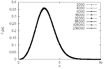
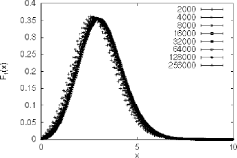
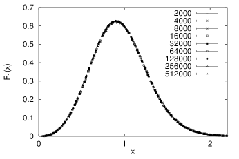
Figure 8.  : The two upper figures depict the measured distributions $G_{V}(r)$ of 2d Euclidean gravity coupled to $c=-2$ conformal matter, defined in terms of the dual link distance and rescaled according to eq. (112) to get $F(x)$, with a shift $\delta=4.5$ (left) and without a shift (right). In the two lower figures, the link distance has been used, again with a shift $\delta=0.5$ (left) and without(right). The best fit for the Hausdorff dimension $d_{h}$ extracted from the data is $3.58\pm 0.01$, in agreement with theoretical predictions [55].

Analogous results hold for branched-polymer systems, whose two-point functions can be calculated exactly. The distance $r$ is in this case given by the (unique) number of links separating each pair of points. For fixed volume $V\to\infty$, we find a universal scaling of the form (112), but now with an (intrinsic) Hausdorff dimension $d_{h}=2$, which also coincides with the value for $d_{H}$. Again a shift in $x$ is needed as a leading finite-size correction to obtain optimal agreement with the theoretical results.

To summarize, measuring $G_{V}(r)$ or $\bar{G}_{V}(r)$ provides an efficient way for determining the Hausdorff dimension $d_{h}$, also in cases where the two-point functions are not known exactly. To take care of short-distance effects, it is important to work with an improved, shifted scaling variable $x_{\delta}$. In practice one measures $G_{V}(r)$ for a number of volumes $V$, and tries to find a best fit to the universal scaling relation (112) by fitting both $\delta$ and $d_{h}$.

Another geometric observable characterizing a compact metric manifold is its spectral dimension, which is related to the diffusion equation and the spectrum of the Laplace operator. If a diffusion process is started with a completely localized initial condition, one can measure the return probability $P(T)$ of a fictitious test particle after “time” $T$. On a fixed continuum geometry, one obtains after averaging over the initial point that

$$P(T)\sim{1\over T^{d_{s}/2}}\sum_{k}a_{k}T^{k},$$ (117)

for small $T$, where the coefficients $a_{k}$ can be expressed in terms of local geometric invariants. We can measure $d_{s}$ also in the discretized theory, but some care must be exercised when comparing with a continuum formula like (117), since it is exactly the short-time limit $T\to 0$ that is ill-defined in the discrete case. This can already be seen in the simple case of diffusion on a discrete one-dimensional line, with a discrete Laplacian and a continuous time. The diffusion equation

$$\frac{d\phi_{i}}{dT}=\frac{\phi_{i+1}+\phi_{i-1}-2\phi_{i}}{2},$$ (118)

with the initial condition $\phi_{i}(0)=\delta_{i0}$ can be solved exactly, yielding

$$P(T)=e^{-T}I_{0}(T)\sim{1\over T^{1/2}}(1+{\cal O}(1/T)),$$ (119)

where $I_{0}(T)$ is the Bessel function. One therefore rederives the correct spectral dimension ($d_{s}=1$) only for large $T$. The short-time behaviour is completely different and dominated by discretization artifacts. For this simple example, one can check numerically the effect of the finite system size, by changing the discrete line to a closed circle with $V$ points. One observes three distinct regions:

• small time $T$, which is similar to the example above, and dominated by discretization effects;

• intermediate $T$, where one obtains the correct value of $d_{s}$; and

• very large $T$, where the system approaches a stationary translation-invariant state.

A similar structure is also expected in less trivial cases, such as simplicial quantum gravity in two dimensions and higher. This behaviour is illustrated in Fig. 9, where we show the results of measuring the spectral dimension for 2d Euclidean quantum gravity coupled to matter fields of various central charges $c$.

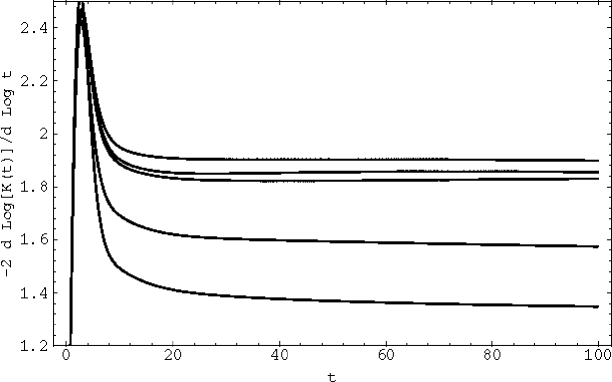
Figure 9.  : The spectral dimension $d_{s}\approx-2d\log P(T)/d\log T$ versus $T$ for $c=0$ (top curve), $c=1/2$, $c=1$, $c=3$ and c=5 (bottom curve) theories coupled to 2d Euclidean quantum gravity. The system size is $V$=16000 triangles.

The measurement of the spectral dimension in 2d Euclidean quantum gravity is a nice illustration of the fruitful interaction between numerical “experiment” and theory. Since the quantum geometry of 2d Euclidean gravity has a fractal Hausdorff dimension $d_{h}\!=\!4$, one could also have expected an anomalous spectral dimension $d_{s}$. However, numerical simulations consistently found that $d_{s}=2$, no matter which field theory was coupled to gravity, as long as the central charge $c$ remained $\leq 1$. This inspired an analytic proof of this value, using continuum conformal Liouville theory and an assumption about finite-size scaling [56, 57]. We should point out that $d_{s}\!=\!2$ does not imply that one cannot see the fractal structure corresponding to $d_{h}\!=\!4$ in the diffusion process. It manifests itself in the relation

$$\langle R\rangle_{T}\sim T^{1/d_{h}}$$ (120)

between the “time” $T$ and the average geodesic distance $R$ diffused in that time. We refer again to [56, 57] for details.

For $c>1$, the numerical estimate was close to $d_{s}=4/3$. Eventually it was proven that generic branched polymers have a spectral dimension $d_{s}=4/3$ [58], thus reconciling theory and numerical results. At the same time, it provided independent evidence that for $c>1$ the space-time degenerates into branched polymers.

We have so far discussed only purely geometric observables. For theories coupled to matter, there will be additional critical exponents characterizing the behaviour of the system close to the critical matter coupling $\beta_{c}$. Near this transition point, we expect to find a divergent correlation length $\xi(\beta)\sim|\beta-\beta_{c}|^{-\nu}$, for some positive $\nu$. Since we always study systems of finite size, we will never observe a genuine phase transition, but merely a pseudo-critical point $\beta_{c}^{*}(V)$, where the linear extension $L$ of the system behaves like $L\sim\xi(\beta)$. For a finite system $L^{d}=V$. A system with a dynamical geometry may possess two scales: one associated with the cosmological constant when $\mu\to\mu_{0}$ and another one related to the matter phase transition. Using standard finite-size scaling arguments, we expect that the measured values of the specific heat $c_{v}$, the magnetization per unit volume $m$, and the magnetic susceptibility $\chi$ at the pseudo-critical point $\beta_{c}^{*}$ behave like

$$c_{v}(\beta_{c}^{*}) \sim V^{\frac{\alpha}{\nu d}},$$

$$m(\beta_{c}^{*}) \sim V^{-\frac{\beta_{m}}{\nu d}},$$

$$\chi(\beta_{c}^{*}) \sim V^{\frac{\gamma_{m}}{\nu d}},$$ (121)

where $\alpha$, $\beta_{m}$ and $\gamma_{m}$ satisfy the scaling relations

$$\alpha+2\beta_{m}+\gamma_{m}=2,~{}~{}~{}~{}~{}~{}2\beta_{m}+\gamma_{m}=\nu d.$$ (122)

For magnetic systems corresponding to $0<c<1$, one knows from analytical calculations the values of the critical exponents as well as the values of the critical points $\beta_{c}$.

A relation between the scalings in the geometric and matter sectors can be obtained by generalizing the two-point functions $G_{\mu}(r)$ and $G_{V}(r)$, to include also correlations between the matter fields at geodesic distance $r$. One example of a quantity of this kind is

$$G_{\mu}^{\{\phi,\psi\}}(r)=\sum_{\tilde{{\cal T}}}\sum_{\phi_{i}}e^{-\mu N_{2}-S_{matter}(\phi_{i})}\sum_{i,j}\phi_{i}\psi_{j}\delta_{D(i,j),r},$$ (123)

which may be expressed as the discrete Laplace transform of a finite-volume correlator,

$$G_{\mu}^{\{\phi,\psi\}}(r)=\sum_{V}e^{-\mu V}G_{V}^{\{\phi,\psi\}}(r).$$ (124)

In this expression, $\phi_{i}$ and $\psi_{j}$ are local functions of the matter or geometric variables at the points $i$ and $j$. A typical example is the spin-spin correlation function of the Ising system. At the combined critical point of the Ising model and the cosmological constant, (123) yields a reparameterization-invariant definition of a matter correlator in quantum gravity. More precisely, the correlation function is that of a $c\!=\!1/2$ conformal field theory coupled to 2d Euclidean quantum gravity. Note also that the previously defined geometric two-point function (106) is a special case of (123), with the unit operator replacing the spin operators.

This construction has provided us with a new understanding of the KPZ-exponents of conformal field theories coupled to gravity. These exponents may be viewed as the “dressed” scaling exponents of the primary fields in the conformal theory. However, before it was realized that they should be analyzed in terms of the definition (123), it was not clear how to generalize the usual flat-space correlators because of the requirement of reparametrization-invariance (see [59, 60] for further discussion). Fig. 10 shows the result of a numerical simulation of the (suitably normalized) spin-spin correlator.

Figure 10.  : The normalized spin-spin correlation function for the Ising model coupled to 2d Euclidean gravity, plotted as a function of the dimensionless length $x=r/N_{T}^{1/d_{h}}$, where $r$ is the geodesic length and $N_{T}$ the space-time volume. The number of triangles $N_{T}$ ranges from 2000 to 256000 and the Hausdorff dimension is $d_{h}=4.0$. The short-distance behaviour is in accordance with KPZ scaling.

We should point out a subtlety in the definition of the correlator (123). If the expectation values of the fields entering are not zero, one might be interested in defining the corresponding connected correlator. However, there is no straightforward way of defining such an object since (123), in addition to the usual average over field configurations, also includes an average over geometry. A discussion of possible definitions of the connected part of the two-point correlators and their scaling properties can be found in [61].

All of the observables introduced above can also be used in numerical simulations of higher-dimensional gravity-matter systems, and – apart from the ones involving baby-universe counting – also for Lorentzian quantum gravity.

5.3 Comments on the 2d results

Our obvious starting point in 2d Euclidean quantum gravity was the measurement of $\gamma_{str}$, in order to compare it with the theoretical prediction for $c<1$, namely,

$$\gamma_{str}=\frac{c-1-\sqrt{(c-1)(c-25)}}{12}.$$ (125)

For $c>1$, this quantity becomes imaginary and its interpretation in terms of Liouville theory breaks down. For $c=1$, logarithmic corrections appear. For a number of special values of $c$, we have explicit discrete models, which at their critical points represent conformal field theories with charge $c$. They are pure 2d gravity ($c=0$, $\gamma_{str}=-1/2$), the Ising model ($c=1/2,~{}\gamma_{str}=-1/3$), the 3-state Potts model ($c=4/5,~{}\gamma_{str}=-1/5$), the 4-state Potts model ($c=1,~{}\gamma_{str}=0$), and a single massless scalar field ($c=1,~{}\gamma_{str}=0$). In all of these cases, formula (125) has been verified with great accuracy. A coupling of several matter fields corresponds to adding their central charges.

Away from their critical points $\beta_{c}$, the finite spin systems approach a pure-gravity behaviour, with $\gamma_{str}\to-1/2$. This observation can be turned into a method for locating $\beta_{c}$, by monitoring the change in $\gamma_{str}$ as the coupling $\beta$ is varied (Fig. 11).

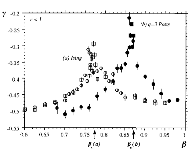
Figure 11.  : Measurements of $\gamma_{str}$ as a function of $\beta$, for the Ising model (white), and the $3$-state Potts model (black), at system sizes $N$ = 1000 (circles) and 2000 (squares).

For all the spin systems, measurements of the magnetic critical exponents defined in (121) are in perfect agreement with the theoretical predictions. We conclude that for the matter models with $0\leq c\leq 1$ which have been used in numerical simulations, the scaling limit of the discretized theory corresponds to a unitary matter model coupled to Liouville gravity.

A somewhat surprising result in this range of $c$ is the numerical value of $d_{h}$ obtained from the scaling of $G_{V}(r)$. For $0\leq c<1$, there are two theoretical predictions for $d_{h}$, namely

$$d_{h}^{(i)}=2\frac{\sqrt{25-c}+\sqrt{49-c}}{\sqrt{25-c}+\sqrt{1-c}},$$ (126)

derived by studying diffusion in a fluctuating geometry, using Liouville theory [55], and

$$d_{h}^{(ii)}=\frac{24}{\sqrt{1-c}\ (\sqrt{1-c}+\sqrt{25-c})},$$ (127)

derived from matrix model considerations [62]. The formulas agree for $c\!=\!0$ (where $d_{h}\!=\!4$), but differ elsewhere. In both derivations there are plausible, but unjustified, assumptions. Neither of them could be confirmed by numerical simulations. Instead, a numerical estimate $d_{h}\simeq 4$ was obtained for all cases with $0\leq c\leq 1$ [51, 59] together with $d_{H}\simeq d_{h}$ [60, 59] from the small-$x$ behaviour of $F(x)$. The numerical errors seem sufficiently small to support the conjecture that $d_{h}=4$ for unitary matter theories coupled to 2d gravity. The spin-spin correlation functions measured for the Ising system ($c=1/2$) at $\beta=\beta_{c}$ seem to indicate that the matter degrees of freedom do not introduce a new scale and that also for these correlations, there is a universal scaling corresponding to $d_{h}\simeq 4$.

Our numerical information for the case $c<0$ is only partial. A special case is $c=-2$, where the simulations can be based on a direct generation of diagrams, instead of Monte Carlo methods. As already mentioned in connection with Fig. 8 this led to $d_{h}=3.58\pm 0.02$, which is very close to the value of $d_{h}=3.561\dots$ predicted by (126). Less conclusive numerical data for $c=-5$ also show agreement with (126). Formula (126) also predicts that $d_{h}=2$ as $c\to-\infty$, which is the expected flat-space behaviour. It thus seems that eq. (126) could be correct for $c\leq 0$. It is still not understood why the formula fails for $0<c\leq 1$.

For $c>1$, the minbu size diverges as $V\to\infty$. Systems with $c>1$ can easily be studied numerically by coupling several copies of spins or scalar fields. In all cases studied, $\gamma_{str}$ was found to be positive and to approach $+1/2$ for $c\simeq 4$ and bigger, suggestive of a branched-polymer system. This interpretation would also agree with the scaling analysis of $G_{V}(r)$ which is consistent with $d_{h}\to 2$, and the measurement of $d_{s}$, consistent with $d_{s}\to 4/3$. It is not clear to what extent the observed behaviour is universal, since the numerical estimates depend on the details of the regularization. For example, the approach to the branched-polymer phase seems slower when regular triangulations $T$ rather than generalized configurations in ${\cal T}$ are used. This could be due to finite-size effects, or alternatively to the presence of other universality classes of branched-polymer systems.

In the 2d Euclidean case, we have learned from both theoretical and numerical investigations that there is only a small “window” of physically sensible theories, by which we mean unitary matter models coupled to gravity. If we move outside this range by adding too many matter fields, the theory breaks down. This indicates that matter and geometry are interacting strongly.

Baby universes play a crucial role in understanding the nature of the spin-gravity interaction, highlighting at the same time the difference between the Euclidean and Lorentzian gravity models. Again the Ising model serves as an ideal illustration. The Ising ground state at zero temperature, for both fixed and fluctuating geometries, is the state where all spins are aligned. Since the energy of a given spin configuration is proportional to the length of the boundary separating spin-up and spin-down regions, the dominant spin configurations at low temperature (equivalently, at large spin coupling) are those with minimal spin boundary lengths.

The lowest spin excitations contributing to the free energy density come from spin clusters with boundaries of minimal length. Unlike on flat, regular lattices, a short spin boundary does not imply that there are few spins inside. On the contrary, the typical situation in Euclidean quantum gravity has an entire baby universe of up-spins, say, on one side of the minimal boundary, and the parent universe with opposite spin orientation on the other, as illustrated in Fig. 12. Since the baby universe can have any size, there is no restriction on the size of spin clusters, even at low temperature. The introduction of a fluctuating geometry with baby universes thus has a strong effect on the matter behaviour. In turn, since short spin boundaries are energetically preferred, the matter has a tendency to “squeeze off” the underlying geometry, generating even more baby universes.

...........................................................................................................................................................................................................................................................................................................................................................................................................................................................................................................................................................................................................................................................................................................................................................................................................................................................................................................................................................................................................................................................................................................................................................................................................................................$-$........................................................................................................................................................................................................................................................................................................................................................................................................................................................................................................................................................................................................................................................................................................................................................................................................$+$          

Figure 12.  : Two spin clusters separated by only two links which form a “bottleneck” on the surface. Two of the four triangles containing one of the two spin-boundary links are also shown.

When more than two Ising models are coupled to 2d Euclidean quantum gravity, the matter-geometry interaction becomes so strong that the geometries degenerate into so-called branched polymers, which can be viewed as infinitely branched trees of baby universes of cut-off size (the lattice spacing $a$). This provides us with an explicit picture of the $c\!=\!1$ barrier of 2d Euclidean quantum gravity. The proliferation of baby universes and its relation to spin clusters are illustrated in Fig. 13.

...............................................................................................................................................................................................................................................................................................................................................................................................................................................................................................................................................................................................................................................................................................................................................................................................................................................................................................................................................................................................................................................................................................................................................................................................................................................................................................................$+$.........................................................................................................................................................................................................................................................................................................................................................................................................................................................................................................................................................................................................................................................................................................................................................................................................................................................................................................................................................................$=$$+$$-$$-$   

Figure 13.  : A surface with a minimal boundary and its recursive decomposition into baby universes associated with spin clusters.

Since baby universes are absent from Lorentzian gravity, its interaction with matter is much weaker. The Ising model on Lorentzian geometries has not yet been solved analytically, but its critical exponents have been determined both by a high-temperature expansion and Monte Carlo techniques [12]. The Hausdorff dimension of space-time is still $d_{h}=2$, and the critical Ising exponents retain the Onsager values found on fixed, regular lattices, in spite of large fluctuations of the geometry. It has also been shown [28] that a particular dimer model coupled to Lorentzian gravity does not change the fractal dimension of the geometry. It is thus tempting to conjecture that the (fractal) dimension of space-time remains equal to 2 as long as the central change of the matter fields is less than or equal to 1.

It is an interesting question whether there is an analogue of the $c\!=\!1$ barrier when sufficiently many matter degrees of freedom (with a sufficiently large central charge $c$) are added. This is indeed what seems to happen. A phase transition in the geometry has been observed when coupling 8 Ising spin copies (corresponding to $c\!=\!4$) to 2d Lorentzian quantum gravity [13]. This effect is illustrated in Fig. 14, where we show typical configurations of the fluctuating Lorentzian geometry in the case of coupling to a single Ising model and to 8 Ising models.

                          

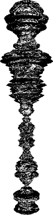
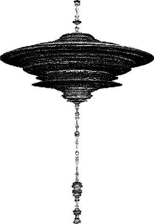
Figure 14.  : Two typical space-time configurations, resulting from the coupling of one Ising model (left) and eight Ising models (right) to Lorentzian gravity.

The one-Ising triangulation is qualitatively very similar to the fluctuating geometry without any Ising spins, but in the case of 8 Ising spins, the effect of the matter is very pronounced. Since the creation of baby-universe branches is by definition forbidden, the only way for the matter to create short spin-boundaries is by squeezing individual spatial slices to a minimal (cut-off) size, producing the long, stalk-like structure seen in Fig. 14. In the remainder of space-time, the spatial slices attain a macroscopic size. On this extended part of the universe, the scaling of the average spatial length in terms of the cosmological constant is anomalous,

$$\left\langle L\right\rangle_{\Lambda}\sim\frac{1}{\Lambda^{2/3}},$$ (128)

which was not the case for $c\leq 1$. Moreover, the critical Ising exponents, when measured on the extended region, are still given by the Onsager values. We therefore have identified an analogue of the $c=1$ barrier, at which a geometric phase transition takes place. However, its effect is much milder than in Euclidean gravity. Ising-life continues even beyond the barrier. This underlines yet again the drastic difference between 2d gravity with and without baby universes.

6 Dynamically triangulated quantum gravity in $d>2$

6.1 Generalization to higher dimensions

The general outline of the simplicial regularization of Euclidean quantum gravity presented above remains true in dimension $d>2$, where the fundamental building blocks are $d$-simplices with $d+1$ vertices. The partition function for dynamically triangulated pure gravity is given by

$$Z=\sum_{\bar{T}}{1\over N_{0}(T)!}e^{-S_{EH}},$$ (129)

where the sum is taken over a class of labelled $d$-dimensional triangulations with spherical topology. In the following, we will be mainly interested in the cases $d=3,4$, where the discretized Einstein-Hilbert action (87) can be written equivalently as

$$S_{EH}=\kappa_{d}N_{d}-\kappa_{0}N_{0},$$ (130)

using the Dehn-Sommerville relations. Since for simplicial manifolds and fixed volume $N_{d}$, the number of vertices has an upper limit $N_{0}\propto N_{d}/d$, the action (130) is bounded for finite volume.

Note that in $d>2$ it is not possible to realize a locally flat geometry by gluing together equilateral simplices. Only in 2d there is a regular tiling of flat space, in which each vertex is shared by six triangles. This happens because the dihedral angle $\theta_{d}$ of each $d$-simplex contributing to the parallel transport around a $(d-2)$-simplex satisfies $\theta_{d}=\arccos 1/d$, which for $d>2$ is not a rational fraction of $2\pi$. However, this is a short-distance property which should become irrelevant in the scaling limit.

In the simplest case of gravity without matter, there are two couplings: $\kappa_{d}$, which is proportional to the cosmological constant, and $\kappa_{0}$, related to the gravitational constant. Both quantities are dimensionless in the lattice formulation, but will get their dimension back through “dimensional transmutation” in the scaling limit, if it exists.

The gravitational state sum is now

$$Z=\sum_{V}e^{-\kappa_{d}V}Z_{V}(\kappa_{0}),$$ (131)

where $V=N_{d}$, and $Z_{V}(\kappa_{0})$ is the partition function at fixed volume. In order for the sum (131) to be well defined, $Z_{V}(\kappa_{0})$ must be exponentially bounded for large $V$,

$$Z_{V}(\kappa_{0})\sim e^{\kappa_{d}^{c}(\kappa_{0})V}z_{V}(\kappa_{0}).$$ (132)

The existence of such a bound has been shown [24, 25], but the form of the subleading terms is at present unknown. A power behaviour of $z_{V}$ leads to a situation similar to (102), but there could in principle also be a logarithmic dependence $\log z_{V}\sim V^{\alpha}$, with $\alpha<1$. For systems with a fixed volume one can replace $Z_{V}$ by $z_{V}$ when averaging over configurations. Note that higher-dimensional gravity with the action (130) resembles a spin system in 2d, with the role of the matter coupling $\beta$ played by $\kappa_{0}$. The cosmological constant will undergo a renormalization according to

$$Z=\sum_{V}e^{-(\kappa_{d}-\kappa_{d}^{c})V}z_{V}(\kappa_{0}),$$ (133)

and $1/(\kappa_{d}-\kappa_{d}^{c})$ gives an estimate of $\left\langle V\right\rangle_{\kappa_{d}}$.

To understand the critical properties of the system defined by (133), one must investigate the limit $V\to\infty$. For large positive $\kappa_{0}$, configurations with many vertices will be favoured. Comparing with the 2d case, we expect this limit to correspond to a branched-polymer phase. Conversely, for large negative $\kappa_{0}$, the system will move towards lower $N_{0}$, leading to “crumpled” configurations. Note that unlike in 2d, $N_{0}$ and $V$ are independent, and $N_{0}$ can be very small, for example, it is easy to find triangulations such that $N_{0}\sim V^{a}$ with $a<1$. The fraction $p(\kappa_{0})=d\left\langle N_{0}\right\rangle_{V}/V$ can be used as an order parameter of the theory, and is related to the average local curvature. It may vary between 0 and 1, corresponding to the two extreme geometric phases. In the limit $p\!=\!0$ ($\kappa_{0}$ small), where the geometry is “crumpled”, there are only a few vertices and one can move from one to another in only a few steps. The Hausdorff dimension of such geometries is large. In the limit $p\!=\!1$ (large $\kappa_{0}$), the number of vertices for a given $V$ is maximal, leading to branched-polymer configurations with Hausdorff dimension two.

Neither of these two limits looks like a promising candidate for a scaling $d$-dimensional quantum theory. Let us compare this situation with that of a 2d spin system. The two extreme phases correspond to the high- and low-temperature regions of the spin model, where also the spin system has no continuum limit. In the high-temperature limit, the spins fluctuate totally randomly, whereas in the low-temperature limit they hardly fluctuate at all. However, there is a critical temperature $T_{c}$ where the spin fluctuations become critical and long-ranged. At $T_{c}$, one can take a continuum limit and recover a $c\!=\!1/2$ conformal field theory. In a similar way one might hope to find a critical gravitational coupling $\kappa_{0}$, where a transition between the two phases of geometries takes place, and where more “reasonable” geometries, exhibiting long-range fluctuations, can be observed. Such a point could serve as a non-perturbative fixed point where a theory of quantum gravity can be defined.

Although the problem of solving higher-dimensional gravity with the simple action (130) is a combinatorial problem which superficially looks quite similar to the 2d case, we still have no hints of how to find an exact solution. There is a mean-field analysis [25, 26] which gives a surprisingly precise description of the phase transition (see also [27]), but most of our understanding of Euclidean dynamical triangulations in $d>2$ comes from performing Monte Carlo simulations, along the lines described in Section 5. Also in these cases a set of ergodic moves is known [46]. Recall that in 2d, one possible set was given by the $(p,q)$-moves, for integer $p,q>0$ and such that $p+q=d+2$. During a $(p,q)$-move, a subcomplex of $p$ simplices is replaced by one of $q$ simplices with the same $(d-1)$-dimensional boundary. This set can be generalized to higher dimensions [64, 65], using the observation that by gluing the two subcomplexes from before and after the move, one obtains the boundary of a $(d+1)$-simplex. The boundary can be divided into two connected parts (a part $X$ and its complement $\bar{X}$) in a finite number of ways. Each move corresponds to replacing some $X\to\bar{X}$. In two dimensions, the boundary is that of a tetrahedron, made of four triangles. It can be divided either into two pairs of two adjacent triangles or into a single triangle and a set of three triangles sharing a vertex of order three.

Performing an analogous construction in 3d, one obtains $(1,4)$- and $(2,3)$-moves, together with their inverses $(4,1)$ and $(3,2)$. The first move inserts a new vertex of order four at the centre of a tetrahedron, thereby creating four new tetrahedra. A $(2,3)$-move takes two tetrahedra which share a triangle, removes this triangle and replaces the two tetrahedra by three tetrahedra, whose common axis (a link of order three) is dual to the removed triangle. Both types of moves are shown in Fig. 15.

$$\raisebox{4.30554pt}{\parbox{99.58464pt}{\mbox{\hbox{\kern-148.1017pt\lower 277.74046pt\hbox{\ignorespaces\ignorespaces\ignorespaces\ignorespaces\ignorespaces\ignorespaces\ignorespaces\ignorespaces\ignorespaces\ignorespaces\ignorespaces\ignorespaces\ignorespaces\ignorespaces\ignorespaces\ignorespaces\ignorespaces\ignorespaces\ignorespaces\kern 198.494pt\raise 379.15196pt\hbox{\thinlinefont.}\kern-198.494pt\ignorespaces\kern 198.22775pt\raise 378.85237pt\hbox{\thinlinefont.}\kern-198.22775pt\ignorespaces\kern 197.9615pt\raise 378.55278pt\hbox{\thinlinefont.}\kern-197.9615pt\ignorespaces\kern 197.69525pt\raise 378.25319pt\hbox{\thinlinefont.}\kern-197.69525pt\ignorespaces\kern 197.429pt\raise 377.9536pt\hbox{\thinlinefont.}\kern-197.429pt\ignorespaces\kern 197.16275pt\raise 377.654pt\hbox{\thinlinefont.}\kern-197.16275pt\ignorespaces\kern 196.8965pt\raise 377.35442pt\hbox{\thinlinefont.}\kern-196.8965pt\ignorespaces\kern 196.63025pt\raise 377.05482pt\hbox{\thinlinefont.}\kern-196.63025pt\ignorespaces\kern 196.364pt\raise 376.75523pt\hbox{\thinlinefont.}\kern-196.364pt\ignorespaces\kern 196.09775pt\raise 376.45564pt\hbox{\thinlinefont.}\kern-196.09775pt\ignorespaces\kern 195.8315pt\raise 376.15605pt\hbox{\thinlinefont.}\kern-195.8315pt\ignorespaces\kern 195.56525pt\raise 375.85646pt\hbox{\thinlinefont.}\kern-195.56525pt\ignorespaces\kern 195.299pt\raise 375.55687pt\hbox{\thinlinefont.}\kern-195.299pt\ignorespaces\kern 195.03275pt\raise 375.25728pt\hbox{\thinlinefont.}\kern-195.03275pt\ignorespaces\kern 194.7665pt\raise 374.95769pt\hbox{\thinlinefont.}\kern-194.7665pt\ignorespaces\kern 194.50024pt\raise 374.6581pt\hbox{\thinlinefont.}\kern-194.50024pt\ignorespaces\kern 194.234pt\raise 374.3585pt\hbox{\thinlinefont.}\kern-194.234pt\ignorespaces\kern 193.96774pt\raise 374.05891pt\hbox{\thinlinefont.}\kern-193.96774pt\ignorespaces\kern 193.70149pt\raise 373.75932pt\hbox{\thinlinefont.}\kern-193.70149pt\ignorespaces\kern 193.43524pt\raise 373.45973pt\hbox{\thinlinefont.}\kern-193.43524pt\ignorespaces\kern 193.16899pt\raise 373.16014pt\hbox{\thinlinefont.}\kern-193.16899pt\ignorespaces\kern 192.90274pt\raise 372.86055pt\hbox{\thinlinefont.}\kern-192.90274pt\ignorespaces\kern 192.63649pt\raise 372.56096pt\hbox{\thinlinefont.}\kern-192.63649pt\ignorespaces\kern 192.37024pt\raise 372.26137pt\hbox{\thinlinefont.}\kern-192.37024pt\ignorespaces\kern 192.10399pt\raise 371.96178pt\hbox{\thinlinefont.}\kern-192.10399pt\ignorespaces\kern 191.83774pt\raise 371.66219pt\hbox{\thinlinefont.}\kern-191.83774pt\ignorespaces\kern 191.57149pt\raise 371.3626pt\hbox{\thinlinefont.}\kern-191.57149pt\ignorespaces\kern 191.30524pt\raise 371.063pt\hbox{\thinlinefont.}\kern-191.30524pt\ignorespaces\kern 191.03899pt\raise 370.76341pt\hbox{\thinlinefont.}\kern-191.03899pt\ignorespaces\kern 190.77274pt\raise 370.46382pt\hbox{\thinlinefont.}\kern-190.77274pt\ignorespaces\kern 190.50648pt\raise 370.16423pt\hbox{\thinlinefont.}\kern-190.50648pt\ignorespaces\kern 190.24023pt\raise 369.86464pt\hbox{\thinlinefont.}\kern-190.24023pt\ignorespaces\kern 189.97398pt\raise 369.56505pt\hbox{\thinlinefont.}\kern-189.97398pt\ignorespaces\kern 189.70773pt\raise 369.26546pt\hbox{\thinlinefont.}\kern-189.70773pt\ignorespaces\kern 189.44148pt\raise 368.96587pt\hbox{\thinlinefont.}\kern-189.44148pt\ignorespaces\kern 189.17523pt\raise 368.66628pt\hbox{\thinlinefont.}\kern-189.17523pt\ignorespaces\kern 188.90898pt\raise 368.36668pt\hbox{\thinlinefont.}\kern-188.90898pt\ignorespaces\kern 188.64273pt\raise 368.0671pt\hbox{\thinlinefont.}\kern-188.64273pt\ignorespaces\kern 188.37648pt\raise 367.7675pt\hbox{\thinlinefont.}\kern-188.37648pt\ignorespaces\kern 188.11023pt\raise 367.46791pt\hbox{\thinlinefont.}\kern-188.11023pt\ignorespaces\kern 187.84398pt\raise 367.16832pt\hbox{\thinlinefont.}\kern-187.84398pt\ignorespaces\kern 187.57773pt\raise 366.86873pt\hbox{\thinlinefont.}\kern-187.57773pt\ignorespaces\kern 187.31148pt\raise 366.56914pt\hbox{\thinlinefont.}\kern-187.31148pt\ignorespaces\kern 187.04523pt\raise 366.26955pt\hbox{\thinlinefont.}\kern-187.04523pt\ignorespaces\kern 186.77898pt\raise 365.96996pt\hbox{\thinlinefont.}\kern-186.77898pt\ignorespaces\kern 186.51273pt\raise 365.67036pt\hbox{\thinlinefont.}\kern-186.51273pt\ignorespaces\kern 186.24648pt\raise 365.37077pt\hbox{\thinlinefont.}\kern-186.24648pt\ignorespaces\kern 185.98022pt\raise 365.07118pt\hbox{\thinlinefont.}\kern-185.98022pt\ignorespaces\kern 185.71397pt\raise 364.77159pt\hbox{\thinlinefont.}\kern-185.71397pt\ignorespaces\kern 185.44772pt\raise 364.472pt\hbox{\thinlinefont.}\kern-185.44772pt\ignorespaces\kern 185.18147pt\raise 364.17241pt\hbox{\thinlinefont.}\kern-185.18147pt\ignorespaces\kern 184.91522pt\raise 363.87282pt\hbox{\thinlinefont.}\kern-184.91522pt\ignorespaces\kern 184.64897pt\raise 363.57323pt\hbox{\thinlinefont.}\kern-184.64897pt\ignorespaces\kern 184.38272pt\raise 363.27364pt\hbox{\thinlinefont.}\kern-184.38272pt\ignorespaces\kern 184.11647pt\raise 362.97404pt\hbox{\thinlinefont.}\kern-184.11647pt\ignorespaces\kern 183.85022pt\raise 362.67445pt\hbox{\thinlinefont.}\kern-183.85022pt\ignorespaces\kern 183.58397pt\raise 362.37486pt\hbox{\thinlinefont.}\kern-183.58397pt\ignorespaces\kern 183.31772pt\raise 362.07527pt\hbox{\thinlinefont.}\kern-183.31772pt\ignorespaces\kern 183.05147pt\raise 361.77568pt\hbox{\thinlinefont.}\kern-183.05147pt\ignorespaces\kern 182.78522pt\raise 361.47609pt\hbox{\thinlinefont.}\kern-182.78522pt\ignorespaces\kern 182.51897pt\raise 361.1765pt\hbox{\thinlinefont.}\kern-182.51897pt\ignorespaces\kern 182.25272pt\raise 360.8769pt\hbox{\thinlinefont.}\kern-182.25272pt\ignorespaces\kern 181.98647pt\raise 360.57732pt\hbox{\thinlinefont.}\kern-181.98647pt\ignorespaces\kern 181.72021pt\raise 360.27773pt\hbox{\thinlinefont.}\kern-181.72021pt\ignorespaces\kern 181.45396pt\raise 359.97813pt\hbox{\thinlinefont.}\kern-181.45396pt\ignorespaces\kern 181.18771pt\raise 359.67854pt\hbox{\thinlinefont.}\kern-181.18771pt\ignorespaces\kern 180.92146pt\raise 359.37895pt\hbox{\thinlinefont.}\kern-180.92146pt\ignorespaces\kern 180.65521pt\raise 359.07936pt\hbox{\thinlinefont.}\kern-180.65521pt\ignorespaces\kern 180.38896pt\raise 358.77977pt\hbox{\thinlinefont.}\kern-180.38896pt\ignorespaces\kern 180.12271pt\raise 358.48018pt\hbox{\thinlinefont.}\kern-180.12271pt\ignorespaces\kern 179.85646pt\raise 358.18059pt\hbox{\thinlinefont.}\kern-179.85646pt\ignorespaces\kern 179.59021pt\raise 357.881pt\hbox{\thinlinefont.}\kern-179.59021pt\ignorespaces\kern 179.32396pt\raise 357.5814pt\hbox{\thinlinefont.}\kern-179.32396pt\ignorespaces\kern 179.05771pt\raise 357.28181pt\hbox{\thinlinefont.}\kern-179.05771pt\ignorespaces\kern 178.79146pt\raise 356.98222pt\hbox{\thinlinefont.}\kern-178.79146pt\ignorespaces\kern 178.5252pt\raise 356.68263pt\hbox{\thinlinefont.}\kern-178.5252pt\ignorespaces\kern 178.25896pt\raise 356.38304pt\hbox{\thinlinefont.}\kern-178.25896pt\ignorespaces\kern 177.9927pt\raise 356.08345pt\hbox{\thinlinefont.}\kern-177.9927pt\ignorespaces\kern 177.72646pt\raise 355.78386pt\hbox{\thinlinefont.}\kern-177.72646pt\ignorespaces\kern 177.4602pt\raise 355.48427pt\hbox{\thinlinefont.}\kern-177.4602pt\ignorespaces\kern 177.19395pt\raise 355.18468pt\hbox{\thinlinefont.}\kern-177.19395pt\ignorespaces\kern 176.9277pt\raise 354.88509pt\hbox{\thinlinefont.}\kern-176.9277pt\ignorespaces\kern 176.66145pt\raise 354.5855pt\hbox{\thinlinefont.}\kern-176.66145pt\ignorespaces\kern 176.3952pt\raise 354.2859pt\hbox{\thinlinefont.}\kern-176.3952pt\ignorespaces\kern 176.12895pt\raise 353.98631pt\hbox{\thinlinefont.}\kern-176.12895pt\ignorespaces\kern 175.8627pt\raise 353.68672pt\hbox{\thinlinefont.}\kern-175.8627pt\ignorespaces\kern 175.59645pt\raise 353.38713pt\hbox{\thinlinefont.}\kern-175.59645pt\ignorespaces\kern 175.3302pt\raise 353.08754pt\hbox{\thinlinefont.}\kern-175.3302pt\ignorespaces\kern 175.06395pt\raise 352.78795pt\hbox{\thinlinefont.}\kern-175.06395pt\ignorespaces\kern 174.7977pt\raise 352.48836pt\hbox{\thinlinefont.}\kern-174.7977pt\ignorespaces\kern 174.53145pt\raise 352.18877pt\hbox{\thinlinefont.}\kern-174.53145pt\ignorespaces\kern 174.2652pt\raise 351.88918pt\hbox{\thinlinefont.}\kern-174.2652pt\ignorespaces\kern 173.99895pt\raise 351.58958pt\hbox{\thinlinefont.}\kern-173.99895pt\ignorespaces\kern 173.7327pt\raise 351.29pt\hbox{\thinlinefont.}\kern-173.7327pt\ignorespaces\kern 173.46645pt\raise 350.9904pt\hbox{\thinlinefont.}\kern-173.46645pt\ignorespaces\kern 173.2002pt\raise 350.69081pt\hbox{\thinlinefont.}\kern-173.2002pt\ignorespaces\kern 172.93394pt\raise 350.39122pt\hbox{\thinlinefont.}\kern-172.93394pt\ignorespaces\kern 172.6677pt\raise 350.09163pt\hbox{\thinlinefont.}\kern-172.6677pt\ignorespaces\kern 172.40144pt\raise 349.79204pt\hbox{\thinlinefont.}\kern-172.40144pt\ignorespaces\kern 172.1352pt\raise 349.49245pt\hbox{\thinlinefont.}\kern-172.1352pt\ignorespaces\kern 171.86894pt\raise 349.19286pt\hbox{\thinlinefont.}\kern-171.86894pt\ignorespaces\kern 171.60269pt\raise 348.89326pt\hbox{\thinlinefont.}\kern-171.60269pt\ignorespaces\kern 171.33644pt\raise 348.59367pt\hbox{\thinlinefont.}\kern-171.33644pt\ignorespaces\kern 171.07019pt\raise 348.29408pt\hbox{\thinlinefont.}\kern-171.07019pt\ignorespaces\kern 170.80394pt\raise 347.99449pt\hbox{\thinlinefont.}\kern-170.80394pt\ignorespaces\kern 170.53769pt\raise 347.6949pt\hbox{\thinlinefont.}\kern-170.53769pt\ignorespaces\kern 170.27144pt\raise 347.39531pt\hbox{\thinlinefont.}\kern-170.27144pt\ignorespaces\kern 170.00519pt\raise 347.09572pt\hbox{\thinlinefont.}\kern-170.00519pt\ignorespaces\kern 169.73894pt\raise 346.79613pt\hbox{\thinlinefont.}\kern-169.73894pt\ignorespaces\kern 169.47269pt\raise 346.49654pt\hbox{\thinlinefont.}\kern-169.47269pt\ignorespaces\kern 169.20644pt\raise 346.19695pt\hbox{\thinlinefont.}\kern-169.20644pt\ignorespaces\kern 168.94019pt\raise 345.89735pt\hbox{\thinlinefont.}\kern-168.94019pt\ignorespaces\kern 168.67393pt\raise 345.59776pt\hbox{\thinlinefont.}\kern-168.67393pt\ignorespaces\kern 168.40768pt\raise 345.29817pt\hbox{\thinlinefont.}\kern-168.40768pt\ignorespaces\kern 168.14143pt\raise 344.99858pt\hbox{\thinlinefont.}\kern-168.14143pt\ignorespaces\kern 167.87518pt\raise 344.69899pt\hbox{\thinlinefont.}\kern-167.87518pt\ignorespaces\kern 167.60893pt\raise 344.3994pt\hbox{\thinlinefont.}\kern-167.60893pt\ignorespaces\kern 167.34268pt\raise 344.09981pt\hbox{\thinlinefont.}\kern-167.34268pt\ignorespaces\kern 167.07643pt\raise 343.80022pt\hbox{\thinlinefont.}\kern-167.07643pt\ignorespaces\kern 166.81018pt\raise 343.50063pt\hbox{\thinlinefont.}\kern-166.81018pt\ignorespaces\kern 166.54393pt\raise 343.20103pt\hbox{\thinlinefont.}\kern-166.54393pt\ignorespaces\kern 166.27768pt\raise 342.90144pt\hbox{\thinlinefont.}\kern-166.27768pt\ignorespaces\kern 166.01143pt\raise 342.60185pt\hbox{\thinlinefont.}\kern-166.01143pt\ignorespaces\kern 165.74518pt\raise 342.30226pt\hbox{\thinlinefont.}\kern-165.74518pt\ignorespaces\kern 165.47893pt\raise 342.00267pt\hbox{\thinlinefont.}\kern-165.47893pt\ignorespaces\kern 165.21268pt\raise 341.70308pt\hbox{\thinlinefont.}\kern-165.21268pt\ignorespaces\kern 164.94643pt\raise 341.40349pt\hbox{\thinlinefont.}\kern-164.94643pt\ignorespaces\kern 164.68018pt\raise 341.1039pt\hbox{\thinlinefont.}\kern-164.68018pt\ignorespaces\kern 164.41393pt\raise 340.8043pt\hbox{\thinlinefont.}\kern-164.41393pt\ignorespaces\kern 164.14767pt\raise 340.50471pt\hbox{\thinlinefont.}\kern-164.14767pt\ignorespaces\kern 163.88142pt\raise 340.20512pt\hbox{\thinlinefont.}\kern-163.88142pt\ignorespaces\kern 163.61517pt\raise 339.90553pt\hbox{\thinlinefont.}\kern-163.61517pt\ignorespaces\kern 163.34892pt\raise 339.60594pt\hbox{\thinlinefont.}\kern-163.34892pt\ignorespaces\kern 163.08267pt\raise 339.30635pt\hbox{\thinlinefont.}\kern-163.08267pt\ignorespaces\kern 162.81642pt\raise 339.00676pt\hbox{\thinlinefont.}\kern-162.81642pt\ignorespaces\kern 162.55017pt\raise 338.70717pt\hbox{\thinlinefont.}\kern-162.55017pt\ignorespaces\kern 162.28392pt\raise 338.40758pt\hbox{\thinlinefont.}\kern-162.28392pt\ignorespaces\kern 162.01767pt\raise 338.10799pt\hbox{\thinlinefont.}\kern-162.01767pt\ignorespaces\kern 161.75142pt\raise 337.8084pt\hbox{\thinlinefont.}\kern-161.75142pt\ignorespaces\kern 161.48517pt\raise 337.5088pt\hbox{\thinlinefont.}\kern-161.48517pt\ignorespaces\kern 161.21892pt\raise 337.20921pt\hbox{\thinlinefont.}\kern-161.21892pt\ignorespaces\kern 160.95267pt\raise 336.90962pt\hbox{\thinlinefont.}\kern-160.95267pt\ignorespaces\kern 160.68642pt\raise 336.61003pt\hbox{\thinlinefont.}\kern-160.68642pt\ignorespaces\kern 160.42017pt\raise 336.31044pt\hbox{\thinlinefont.}\kern-160.42017pt\ignorespaces\kern 160.15392pt\raise 336.01085pt\hbox{\thinlinefont.}\kern-160.15392pt\ignorespaces\kern 159.88766pt\raise 335.71126pt\hbox{\thinlinefont.}\kern-159.88766pt\ignorespaces\kern 159.62141pt\raise 335.41167pt\hbox{\thinlinefont.}\kern-159.62141pt\ignorespaces\kern 159.35516pt\raise 335.11208pt\hbox{\thinlinefont.}\kern-159.35516pt\ignorespaces\kern 159.08891pt\raise 334.81248pt\hbox{\thinlinefont.}\kern-159.08891pt\ignorespaces\kern 158.82266pt\raise 334.5129pt\hbox{\thinlinefont.}\kern-158.82266pt\ignorespaces\kern 158.55641pt\raise 334.2133pt\hbox{\thinlinefont.}\kern-158.55641pt\ignorespaces\kern 158.29016pt\raise 333.91371pt\hbox{\thinlinefont.}\kern-158.29016pt\ignorespaces\kern 158.02391pt\raise 333.61412pt\hbox{\thinlinefont.}\kern-158.02391pt\ignorespaces\kern 157.75766pt\raise 333.31453pt\hbox{\thinlinefont.}\kern-157.75766pt\ignorespaces\kern 157.49141pt\raise 333.01494pt\hbox{\thinlinefont.}\kern-157.49141pt\ignorespaces\kern 157.22516pt\raise 332.71535pt\hbox{\thinlinefont.}\kern-157.22516pt\ignorespaces\kern 156.95891pt\raise 332.41576pt\hbox{\thinlinefont.}\kern-156.95891pt\ignorespaces\kern 156.69266pt\raise 332.11617pt\hbox{\thinlinefont.}\kern-156.69266pt\ignorespaces\kern 156.4264pt\raise 331.81657pt\hbox{\thinlinefont.}\kern-156.4264pt\ignorespaces\kern 156.16016pt\raise 331.51698pt\hbox{\thinlinefont.}\kern-156.16016pt\ignorespaces\kern 155.8939pt\raise 331.21739pt\hbox{\thinlinefont.}\kern-155.8939pt\ignorespaces\kern 155.62766pt\raise 330.9178pt\hbox{\thinlinefont.}\kern-155.62766pt\ignorespaces\kern 155.3614pt\raise 330.61821pt\hbox{\thinlinefont.}\kern-155.3614pt\ignorespaces\kern 155.09515pt\raise 330.31862pt\hbox{\thinlinefont.}\kern-155.09515pt\ignorespaces\kern 154.8289pt\raise 330.01903pt\hbox{\thinlinefont.}\kern-154.8289pt\ignorespaces\kern 154.56265pt\raise 329.71944pt\hbox{\thinlinefont.}\kern-154.56265pt\ignorespaces\kern 154.2964pt\raise 329.41985pt\hbox{\thinlinefont.}\kern-154.2964pt\ignorespaces\kern 154.03015pt\raise 329.12025pt\hbox{\thinlinefont.}\kern-154.03015pt\ignorespaces\kern 153.7639pt\raise 328.82066pt\hbox{\thinlinefont.}\kern-153.7639pt\ignorespaces\kern 153.49765pt\raise 328.52107pt\hbox{\thinlinefont.}\kern-153.49765pt\ignorespaces\kern 153.2314pt\raise 328.22148pt\hbox{\thinlinefont.}\kern-153.2314pt\ignorespaces\kern 152.96515pt\raise 327.92189pt\hbox{\thinlinefont.}\kern-152.96515pt\ignorespaces\kern 152.6989pt\raise 327.6223pt\hbox{\thinlinefont.}\kern-152.6989pt\ignorespaces\kern 152.43265pt\raise 327.32271pt\hbox{\thinlinefont.}\kern-152.43265pt\ignorespaces\kern 152.1664pt\raise 327.02312pt\hbox{\thinlinefont.}\kern-152.1664pt\ignorespaces\kern 151.90015pt\raise 326.72353pt\hbox{\thinlinefont.}\kern-151.90015pt\ignorespaces\kern 151.6339pt\raise 326.42393pt\hbox{\thinlinefont.}\kern-151.6339pt\ignorespaces\kern 151.36765pt\raise 326.12434pt\hbox{\thinlinefont.}\kern-151.36765pt\ignorespaces\kern 151.1014pt\raise 325.82475pt\hbox{\thinlinefont.}\kern-151.1014pt\ignorespaces\kern 150.83514pt\raise 325.52516pt\hbox{\thinlinefont.}\kern-150.83514pt\ignorespaces\kern 150.5689pt\raise 325.22557pt\hbox{\thinlinefont.}\kern-150.5689pt\ignorespaces\kern 150.30264pt\raise 324.92598pt\hbox{\thinlinefont.}\kern-150.30264pt\ignorespaces\kern 150.03639pt\raise 324.62639pt\hbox{\thinlinefont.}\kern-150.03639pt\ignorespaces\kern 149.77014pt\raise 324.3268pt\hbox{\thinlinefont.}\kern-149.77014pt\ignorespaces\kern 149.50389pt\raise 324.0272pt\hbox{\thinlinefont.}\kern-149.50389pt\ignorespaces\kern 149.23764pt\raise 323.72762pt\hbox{\thinlinefont.}\kern-149.23764pt\ignorespaces\kern 148.97139pt\raise 323.42802pt\hbox{\thinlinefont.}\kern-148.97139pt\ignorespaces\kern 148.70514pt\raise 323.12843pt\hbox{\thinlinefont.}\kern-148.70514pt\ignorespaces\kern 148.43889pt\raise 322.82884pt\hbox{\thinlinefont.}\kern-148.43889pt\ignorespaces\kern 148.17264pt\raise 322.52925pt\hbox{\thinlinefont.}\kern-148.17264pt\ignorespaces\kern 147.90639pt\raise 322.22966pt\hbox{\thinlinefont.}\kern-147.90639pt\ignorespaces\ignorespaces\ignorespaces\ignorespaces\ignorespaces\ignorespaces\ignorespaces\ignorespaces\ignorespaces\ignorespaces\ignorespaces\ignorespaces\ignorespaces\ignorespaces\kern 198.494pt\raise 379.15196pt\hbox{\thinlinefont.}\kern-198.494pt\ignorespaces\kern 198.71588pt\raise 378.81909pt\hbox{\thinlinefont.}\kern-198.71588pt\ignorespaces\kern 198.93776pt\raise 378.48622pt\hbox{\thinlinefont.}\kern-198.93776pt\ignorespaces\kern 199.15964pt\raise 378.15335pt\hbox{\thinlinefont.}\kern-199.15964pt\ignorespaces\kern 199.38152pt\raise 377.82048pt\hbox{\thinlinefont.}\kern-199.38152pt\ignorespaces\kern 199.6034pt\raise 377.48761pt\hbox{\thinlinefont.}\kern-199.6034pt\ignorespaces\kern 199.82527pt\raise 377.15474pt\hbox{\thinlinefont.}\kern-199.82527pt\ignorespaces\kern 200.04715pt\raise 376.82187pt\hbox{\thinlinefont.}\kern-200.04715pt\ignorespaces\kern 200.26903pt\raise 376.489pt\hbox{\thinlinefont.}\kern-200.26903pt\ignorespaces\kern 200.4909pt\raise 376.15613pt\hbox{\thinlinefont.}\kern-200.4909pt\ignorespaces\kern 200.71278pt\raise 375.82326pt\hbox{\thinlinefont.}\kern-200.71278pt\ignorespaces\kern 200.93466pt\raise 375.49039pt\hbox{\thinlinefont.}\kern-200.93466pt\ignorespaces\kern 201.15654pt\raise 375.15752pt\hbox{\thinlinefont.}\kern-201.15654pt\ignorespaces\kern 201.37842pt\raise 374.82465pt\hbox{\thinlinefont.}\kern-201.37842pt\ignorespaces\kern 201.6003pt\raise 374.49178pt\hbox{\thinlinefont.}\kern-201.6003pt\ignorespaces\kern 201.82217pt\raise 374.1589pt\hbox{\thinlinefont.}\kern-201.82217pt\ignorespaces\kern 202.04405pt\raise 373.82603pt\hbox{\thinlinefont.}\kern-202.04405pt\ignorespaces\kern 202.26593pt\raise 373.49316pt\hbox{\thinlinefont.}\kern-202.26593pt\ignorespaces\kern 202.48781pt\raise 373.1603pt\hbox{\thinlinefont.}\kern-202.48781pt\ignorespaces\kern 202.70969pt\raise 372.82742pt\hbox{\thinlinefont.}\kern-202.70969pt\ignorespaces\kern 202.93156pt\raise 372.49455pt\hbox{\thinlinefont.}\kern-202.93156pt\ignorespaces\kern 203.15344pt\raise 372.16168pt\hbox{\thinlinefont.}\kern-203.15344pt\ignorespaces\kern 203.37532pt\raise 371.82881pt\hbox{\thinlinefont.}\kern-203.37532pt\ignorespaces\kern 203.5972pt\raise 371.49594pt\hbox{\thinlinefont.}\kern-203.5972pt\ignorespaces\kern 203.81908pt\raise 371.16307pt\hbox{\thinlinefont.}\kern-203.81908pt\ignorespaces\kern 204.04095pt\raise 370.8302pt\hbox{\thinlinefont.}\kern-204.04095pt\ignorespaces\kern 204.26283pt\raise 370.49733pt\hbox{\thinlinefont.}\kern-204.26283pt\ignorespaces\kern 204.48471pt\raise 370.16446pt\hbox{\thinlinefont.}\kern-204.48471pt\ignorespaces\kern 204.70659pt\raise 369.83159pt\hbox{\thinlinefont.}\kern-204.70659pt\ignorespaces\kern 204.92847pt\raise 369.49872pt\hbox{\thinlinefont.}\kern-204.92847pt\ignorespaces\kern 205.15034pt\raise 369.16585pt\hbox{\thinlinefont.}\kern-205.15034pt\ignorespaces\kern 205.37222pt\raise 368.83298pt\hbox{\thinlinefont.}\kern-205.37222pt\ignorespaces\kern 205.5941pt\raise 368.5001pt\hbox{\thinlinefont.}\kern-205.5941pt\ignorespaces\kern 205.81598pt\raise 368.16724pt\hbox{\thinlinefont.}\kern-205.81598pt\ignorespaces\kern 206.03786pt\raise 367.83437pt\hbox{\thinlinefont.}\kern-206.03786pt\ignorespaces\kern 206.25974pt\raise 367.5015pt\hbox{\thinlinefont.}\kern-206.25974pt\ignorespaces\kern 206.48161pt\raise 367.16862pt\hbox{\thinlinefont.}\kern-206.48161pt\ignorespaces\kern 206.70349pt\raise 366.83575pt\hbox{\thinlinefont.}\kern-206.70349pt\ignorespaces\kern 206.92537pt\raise 366.50288pt\hbox{\thinlinefont.}\kern-206.92537pt\ignorespaces\kern 207.14725pt\raise 366.17001pt\hbox{\thinlinefont.}\kern-207.14725pt\ignorespaces\kern 207.36913pt\raise 365.83714pt\hbox{\thinlinefont.}\kern-207.36913pt\ignorespaces\kern 207.591pt\raise 365.50427pt\hbox{\thinlinefont.}\kern-207.591pt\ignorespaces\kern 207.81288pt\raise 365.1714pt\hbox{\thinlinefont.}\kern-207.81288pt\ignorespaces\kern 208.03476pt\raise 364.83853pt\hbox{\thinlinefont.}\kern-208.03476pt\ignorespaces\kern 208.25664pt\raise 364.50566pt\hbox{\thinlinefont.}\kern-208.25664pt\ignorespaces\kern 208.47852pt\raise 364.17279pt\hbox{\thinlinefont.}\kern-208.47852pt\ignorespaces\kern 208.7004pt\raise 363.83992pt\hbox{\thinlinefont.}\kern-208.7004pt\ignorespaces\kern 208.92227pt\raise 363.50705pt\hbox{\thinlinefont.}\kern-208.92227pt\ignorespaces\kern 209.14415pt\raise 363.17418pt\hbox{\thinlinefont.}\kern-209.14415pt\ignorespaces\kern 209.36603pt\raise 362.84131pt\hbox{\thinlinefont.}\kern-209.36603pt\ignorespaces\kern 209.5879pt\raise 362.50844pt\hbox{\thinlinefont.}\kern-209.5879pt\ignorespaces\kern 209.80978pt\raise 362.17557pt\hbox{\thinlinefont.}\kern-209.80978pt\ignorespaces\kern 210.03166pt\raise 361.8427pt\hbox{\thinlinefont.}\kern-210.03166pt\ignorespaces\kern 210.25354pt\raise 361.50983pt\hbox{\thinlinefont.}\kern-210.25354pt\ignorespaces\kern 210.47542pt\raise 361.17696pt\hbox{\thinlinefont.}\kern-210.47542pt\ignorespaces\kern 210.6973pt\raise 360.84409pt\hbox{\thinlinefont.}\kern-210.6973pt\ignorespaces\kern 210.91917pt\raise 360.51122pt\hbox{\thinlinefont.}\kern-210.91917pt\ignorespaces\kern 211.14105pt\raise 360.17834pt\hbox{\thinlinefont.}\kern-211.14105pt\ignorespaces\kern 211.36293pt\raise 359.84547pt\hbox{\thinlinefont.}\kern-211.36293pt\ignorespaces\kern 211.58481pt\raise 359.5126pt\hbox{\thinlinefont.}\kern-211.58481pt\ignorespaces\kern 211.80669pt\raise 359.17973pt\hbox{\thinlinefont.}\kern-211.80669pt\ignorespaces\kern 212.02856pt\raise 358.84686pt\hbox{\thinlinefont.}\kern-212.02856pt\ignorespaces\kern 212.25044pt\raise 358.51399pt\hbox{\thinlinefont.}\kern-212.25044pt\ignorespaces\kern 212.47232pt\raise 358.18112pt\hbox{\thinlinefont.}\kern-212.47232pt\ignorespaces\kern 212.6942pt\raise 357.84825pt\hbox{\thinlinefont.}\kern-212.6942pt\ignorespaces\kern 212.91608pt\raise 357.51538pt\hbox{\thinlinefont.}\kern-212.91608pt\ignorespaces\kern 213.13795pt\raise 357.18251pt\hbox{\thinlinefont.}\kern-213.13795pt\ignorespaces\kern 213.35983pt\raise 356.84964pt\hbox{\thinlinefont.}\kern-213.35983pt\ignorespaces\kern 213.58171pt\raise 356.51677pt\hbox{\thinlinefont.}\kern-213.58171pt\ignorespaces\kern 213.80359pt\raise 356.1839pt\hbox{\thinlinefont.}\kern-213.80359pt\ignorespaces\kern 214.02547pt\raise 355.85103pt\hbox{\thinlinefont.}\kern-214.02547pt\ignorespaces\kern 214.24734pt\raise 355.51816pt\hbox{\thinlinefont.}\kern-214.24734pt\ignorespaces\kern 214.46922pt\raise 355.18529pt\hbox{\thinlinefont.}\kern-214.46922pt\ignorespaces\kern 214.6911pt\raise 354.85242pt\hbox{\thinlinefont.}\kern-214.6911pt\ignorespaces\kern 214.91298pt\raise 354.51955pt\hbox{\thinlinefont.}\kern-214.91298pt\ignorespaces\kern 215.13486pt\raise 354.18668pt\hbox{\thinlinefont.}\kern-215.13486pt\ignorespaces\kern 215.35674pt\raise 353.8538pt\hbox{\thinlinefont.}\kern-215.35674pt\ignorespaces\kern 215.57861pt\raise 353.52094pt\hbox{\thinlinefont.}\kern-215.57861pt\ignorespaces\kern 215.80049pt\raise 353.18806pt\hbox{\thinlinefont.}\kern-215.80049pt\ignorespaces\kern 216.02237pt\raise 352.8552pt\hbox{\thinlinefont.}\kern-216.02237pt\ignorespaces\kern 216.24425pt\raise 352.52232pt\hbox{\thinlinefont.}\kern-216.24425pt\ignorespaces\kern 216.46613pt\raise 352.18945pt\hbox{\thinlinefont.}\kern-216.46613pt\ignorespaces\kern 216.688pt\raise 351.85658pt\hbox{\thinlinefont.}\kern-216.688pt\ignorespaces\kern 216.90988pt\raise 351.52371pt\hbox{\thinlinefont.}\kern-216.90988pt\ignorespaces\kern 217.13176pt\raise 351.19084pt\hbox{\thinlinefont.}\kern-217.13176pt\ignorespaces\kern 217.35364pt\raise 350.85797pt\hbox{\thinlinefont.}\kern-217.35364pt\ignorespaces\kern 217.57552pt\raise 350.5251pt\hbox{\thinlinefont.}\kern-217.57552pt\ignorespaces\kern 217.7974pt\raise 350.19223pt\hbox{\thinlinefont.}\kern-217.7974pt\ignorespaces\kern 218.01927pt\raise 349.85936pt\hbox{\thinlinefont.}\kern-218.01927pt\ignorespaces\kern 218.24115pt\raise 349.52649pt\hbox{\thinlinefont.}\kern-218.24115pt\ignorespaces\kern 218.46303pt\raise 349.19362pt\hbox{\thinlinefont.}\kern-218.46303pt\ignorespaces\kern 218.6849pt\raise 348.86075pt\hbox{\thinlinefont.}\kern-218.6849pt\ignorespaces\kern 218.90678pt\raise 348.52788pt\hbox{\thinlinefont.}\kern-218.90678pt\ignorespaces\kern 219.12866pt\raise 348.195pt\hbox{\thinlinefont.}\kern-219.12866pt\ignorespaces\kern 219.35054pt\raise 347.86214pt\hbox{\thinlinefont.}\kern-219.35054pt\ignorespaces\kern 219.57242pt\raise 347.52927pt\hbox{\thinlinefont.}\kern-219.57242pt\ignorespaces\kern 219.7943pt\raise 347.1964pt\hbox{\thinlinefont.}\kern-219.7943pt\ignorespaces\kern 220.01617pt\raise 346.86353pt\hbox{\thinlinefont.}\kern-220.01617pt\ignorespaces\kern 220.23805pt\raise 346.53065pt\hbox{\thinlinefont.}\kern-220.23805pt\ignorespaces\kern 220.45993pt\raise 346.19778pt\hbox{\thinlinefont.}\kern-220.45993pt\ignorespaces\kern 220.68181pt\raise 345.86491pt\hbox{\thinlinefont.}\kern-220.68181pt\ignorespaces\kern 220.90369pt\raise 345.53204pt\hbox{\thinlinefont.}\kern-220.90369pt\ignorespaces\kern 221.12556pt\raise 345.19917pt\hbox{\thinlinefont.}\kern-221.12556pt\ignorespaces\kern 221.34744pt\raise 344.8663pt\hbox{\thinlinefont.}\kern-221.34744pt\ignorespaces\kern 221.56932pt\raise 344.53343pt\hbox{\thinlinefont.}\kern-221.56932pt\ignorespaces\kern 221.7912pt\raise 344.20056pt\hbox{\thinlinefont.}\kern-221.7912pt\ignorespaces\kern 222.01308pt\raise 343.86769pt\hbox{\thinlinefont.}\kern-222.01308pt\ignorespaces\kern 222.23495pt\raise 343.53482pt\hbox{\thinlinefont.}\kern-222.23495pt\ignorespaces\kern 222.45683pt\raise 343.20195pt\hbox{\thinlinefont.}\kern-222.45683pt\ignorespaces\kern 222.67871pt\raise 342.86908pt\hbox{\thinlinefont.}\kern-222.67871pt\ignorespaces\kern 222.90059pt\raise 342.53621pt\hbox{\thinlinefont.}\kern-222.90059pt\ignorespaces\kern 223.12247pt\raise 342.20334pt\hbox{\thinlinefont.}\kern-223.12247pt\ignorespaces\kern 223.34435pt\raise 341.87047pt\hbox{\thinlinefont.}\kern-223.34435pt\ignorespaces\kern 223.56622pt\raise 341.5376pt\hbox{\thinlinefont.}\kern-223.56622pt\ignorespaces\kern 223.7881pt\raise 341.20473pt\hbox{\thinlinefont.}\kern-223.7881pt\ignorespaces\kern 224.00998pt\raise 340.87186pt\hbox{\thinlinefont.}\kern-224.00998pt\ignorespaces\kern 224.23186pt\raise 340.53899pt\hbox{\thinlinefont.}\kern-224.23186pt\ignorespaces\kern 224.45374pt\raise 340.20612pt\hbox{\thinlinefont.}\kern-224.45374pt\ignorespaces\kern 224.67561pt\raise 339.87325pt\hbox{\thinlinefont.}\kern-224.67561pt\ignorespaces\kern 224.89749pt\raise 339.54037pt\hbox{\thinlinefont.}\kern-224.89749pt\ignorespaces\kern 225.11937pt\raise 339.2075pt\hbox{\thinlinefont.}\kern-225.11937pt\ignorespaces\kern 225.34125pt\raise 338.87463pt\hbox{\thinlinefont.}\kern-225.34125pt\ignorespaces\kern 225.56313pt\raise 338.54176pt\hbox{\thinlinefont.}\kern-225.56313pt\ignorespaces\kern 225.785pt\raise 338.2089pt\hbox{\thinlinefont.}\kern-225.785pt\ignorespaces\kern 226.00688pt\raise 337.87602pt\hbox{\thinlinefont.}\kern-226.00688pt\ignorespaces\kern 226.22876pt\raise 337.54315pt\hbox{\thinlinefont.}\kern-226.22876pt\ignorespaces\kern 226.45064pt\raise 337.21028pt\hbox{\thinlinefont.}\kern-226.45064pt\ignorespaces\kern 226.67252pt\raise 336.87741pt\hbox{\thinlinefont.}\kern-226.67252pt\ignorespaces\kern 226.8944pt\raise 336.54454pt\hbox{\thinlinefont.}\kern-226.8944pt\ignorespaces\kern 227.11627pt\raise 336.21167pt\hbox{\thinlinefont.}\kern-227.11627pt\ignorespaces\kern 227.33815pt\raise 335.8788pt\hbox{\thinlinefont.}\kern-227.33815pt\ignorespaces\kern 227.56003pt\raise 335.54593pt\hbox{\thinlinefont.}\kern-227.56003pt\ignorespaces\kern 227.7819pt\raise 335.21306pt\hbox{\thinlinefont.}\kern-227.7819pt\ignorespaces\kern 228.00378pt\raise 334.88019pt\hbox{\thinlinefont.}\kern-228.00378pt\ignorespaces\kern 228.22566pt\raise 334.54732pt\hbox{\thinlinefont.}\kern-228.22566pt\ignorespaces\kern 228.44754pt\raise 334.21445pt\hbox{\thinlinefont.}\kern-228.44754pt\ignorespaces\kern 228.66942pt\raise 333.88158pt\hbox{\thinlinefont.}\kern-228.66942pt\ignorespaces\kern 228.8913pt\raise 333.5487pt\hbox{\thinlinefont.}\kern-228.8913pt\ignorespaces\kern 229.11317pt\raise 333.21584pt\hbox{\thinlinefont.}\kern-229.11317pt\ignorespaces\kern 229.33505pt\raise 332.88297pt\hbox{\thinlinefont.}\kern-229.33505pt\ignorespaces\kern 229.55693pt\raise 332.5501pt\hbox{\thinlinefont.}\kern-229.55693pt\ignorespaces\kern 229.77881pt\raise 332.21722pt\hbox{\thinlinefont.}\kern-229.77881pt\ignorespaces\kern 230.00069pt\raise 331.88435pt\hbox{\thinlinefont.}\kern-230.00069pt\ignorespaces\kern 230.22256pt\raise 331.55148pt\hbox{\thinlinefont.}\kern-230.22256pt\ignorespaces\kern 230.44444pt\raise 331.21861pt\hbox{\thinlinefont.}\kern-230.44444pt\ignorespaces\kern 230.66632pt\raise 330.88574pt\hbox{\thinlinefont.}\kern-230.66632pt\ignorespaces\kern 230.8882pt\raise 330.55287pt\hbox{\thinlinefont.}\kern-230.8882pt\ignorespaces\kern 231.11008pt\raise 330.22pt\hbox{\thinlinefont.}\kern-231.11008pt\ignorespaces\kern 231.33195pt\raise 329.88713pt\hbox{\thinlinefont.}\kern-231.33195pt\ignorespaces\kern 231.55383pt\raise 329.55426pt\hbox{\thinlinefont.}\kern-231.55383pt\ignorespaces\kern 231.77571pt\raise 329.22139pt\hbox{\thinlinefont.}\kern-231.77571pt\ignorespaces\kern 231.99759pt\raise 328.88852pt\hbox{\thinlinefont.}\kern-231.99759pt\ignorespaces\kern 232.21947pt\raise 328.55565pt\hbox{\thinlinefont.}\kern-232.21947pt\ignorespaces\kern 232.44135pt\raise 328.22278pt\hbox{\thinlinefont.}\kern-232.44135pt\ignorespaces\kern 232.66322pt\raise 327.88991pt\hbox{\thinlinefont.}\kern-232.66322pt\ignorespaces\kern 232.8851pt\raise 327.55704pt\hbox{\thinlinefont.}\kern-232.8851pt\ignorespaces\kern 233.10698pt\raise 327.22417pt\hbox{\thinlinefont.}\kern-233.10698pt\ignorespaces\kern 233.32886pt\raise 326.8913pt\hbox{\thinlinefont.}\kern-233.32886pt\ignorespaces\kern 233.55074pt\raise 326.55843pt\hbox{\thinlinefont.}\kern-233.55074pt\ignorespaces\kern 233.77261pt\raise 326.22556pt\hbox{\thinlinefont.}\kern-233.77261pt\ignorespaces\kern 233.99449pt\raise 325.89268pt\hbox{\thinlinefont.}\kern-233.99449pt\ignorespaces\kern 234.21637pt\raise 325.55981pt\hbox{\thinlinefont.}\kern-234.21637pt\ignorespaces\kern 234.43825pt\raise 325.22694pt\hbox{\thinlinefont.}\kern-234.43825pt\ignorespaces\kern 234.66013pt\raise 324.89407pt\hbox{\thinlinefont.}\kern-234.66013pt\ignorespaces\kern 234.882pt\raise 324.5612pt\hbox{\thinlinefont.}\kern-234.882pt\ignorespaces\kern 235.10388pt\raise 324.22833pt\hbox{\thinlinefont.}\kern-235.10388pt\ignorespaces\kern 235.32576pt\raise 323.89546pt\hbox{\thinlinefont.}\kern-235.32576pt\ignorespaces\kern 235.54764pt\raise 323.56259pt\hbox{\thinlinefont.}\kern-235.54764pt\ignorespaces\kern 235.76952pt\raise 323.22972pt\hbox{\thinlinefont.}\kern-235.76952pt\ignorespaces\kern 235.9914pt\raise 322.89685pt\hbox{\thinlinefont.}\kern-235.9914pt\ignorespaces\kern 236.21327pt\raise 322.56398pt\hbox{\thinlinefont.}\kern-236.21327pt\ignorespaces\kern 236.43515pt\raise 322.23111pt\hbox{\thinlinefont.}\kern-236.43515pt\ignorespaces\ignorespaces\ignorespaces\ignorespaces\ignorespaces\ignorespaces\ignorespaces\ignorespaces\ignorespaces\ignorespaces\ignorespaces\ignorespaces\ignorespaces\ignorespaces\ignorespaces\ignorespaces\kern 147.90506pt\raise 322.2296pt\hbox{\thinlinefont.}\kern-147.90506pt\ignorespaces\ignorespaces\kern 148.30492pt\raise 322.2296pt\hbox{\thinlinefont.}\kern-148.30492pt\ignorespaces\ignorespaces\kern 148.70477pt\raise 322.2296pt\hbox{\thinlinefont.}\kern-148.70477pt\ignorespaces\ignorespaces\kern 149.10463pt\raise 322.2296pt\hbox{\thinlinefont.}\kern-149.10463pt\ignorespaces\ignorespaces\kern 149.50449pt\raise 322.2296pt\hbox{\thinlinefont.}\kern-149.50449pt\ignorespaces\ignorespaces\kern 149.90434pt\raise 322.2296pt\hbox{\thinlinefont.}\kern-149.90434pt\ignorespaces\ignorespaces\kern 150.3042pt\raise 322.2296pt\hbox{\thinlinefont.}\kern-150.3042pt\ignorespaces\ignorespaces\kern 150.70406pt\raise 322.2296pt\hbox{\thinlinefont.}\kern-150.70406pt\ignorespaces\ignorespaces\kern 151.10391pt\raise 322.2296pt\hbox{\thinlinefont.}\kern-151.10391pt\ignorespaces\ignorespaces\kern 151.50377pt\raise 322.2296pt\hbox{\thinlinefont.}\kern-151.50377pt\ignorespaces\ignorespaces\ignorespaces\ignorespaces\kern 155.13084pt\raise 322.2296pt\hbox{\thinlinefont.}\kern-155.13084pt\ignorespaces\ignorespaces\kern 155.5307pt\raise 322.2296pt\hbox{\thinlinefont.}\kern-155.5307pt\ignorespaces\ignorespaces\kern 155.93192pt\raise 322.2296pt\hbox{\thinlinefont.}\kern-155.93192pt\ignorespaces\ignorespaces\kern 156.33177pt\raise 322.2296pt\hbox{\thinlinefont.}\kern-156.33177pt\ignorespaces\ignorespaces\kern 156.73163pt\raise 322.2296pt\hbox{\thinlinefont.}\kern-156.73163pt\ignorespaces\ignorespaces\kern 157.13148pt\raise 322.2296pt\hbox{\thinlinefont.}\kern-157.13148pt\ignorespaces\ignorespaces\kern 157.53134pt\raise 322.2296pt\hbox{\thinlinefont.}\kern-157.53134pt\ignorespaces\ignorespaces\kern 157.9312pt\raise 322.2296pt\hbox{\thinlinefont.}\kern-157.9312pt\ignorespaces\ignorespaces\kern 158.33105pt\raise 322.2296pt\hbox{\thinlinefont.}\kern-158.33105pt\ignorespaces\ignorespaces\kern 158.73091pt\raise 322.2296pt\hbox{\thinlinefont.}\kern-158.73091pt\ignorespaces\ignorespaces\ignorespaces\ignorespaces\kern 162.35799pt\raise 322.2296pt\hbox{\thinlinefont.}\kern-162.35799pt\ignorespaces\ignorespaces\kern 162.75784pt\raise 322.2296pt\hbox{\thinlinefont.}\kern-162.75784pt\ignorespaces\ignorespaces\kern 163.1577pt\raise 322.2296pt\hbox{\thinlinefont.}\kern-163.1577pt\ignorespaces\ignorespaces\kern 163.55756pt\raise 322.2296pt\hbox{\thinlinefont.}\kern-163.55756pt\ignorespaces\ignorespaces\kern 163.95877pt\raise 322.2296pt\hbox{\thinlinefont.}\kern-163.95877pt\ignorespaces\ignorespaces\kern 164.35863pt\raise 322.2296pt\hbox{\thinlinefont.}\kern-164.35863pt\ignorespaces\ignorespaces\kern 164.75848pt\raise 322.2296pt\hbox{\thinlinefont.}\kern-164.75848pt\ignorespaces\ignorespaces\kern 165.15834pt\raise 322.2296pt\hbox{\thinlinefont.}\kern-165.15834pt\ignorespaces\ignorespaces\kern 165.5582pt\raise 322.2296pt\hbox{\thinlinefont.}\kern-165.5582pt\ignorespaces\ignorespaces\kern 165.95805pt\raise 322.2296pt\hbox{\thinlinefont.}\kern-165.95805pt\ignorespaces\ignorespaces\ignorespaces\ignorespaces\kern 169.58514pt\raise 322.2296pt\hbox{\thinlinefont.}\kern-169.58514pt\ignorespaces\ignorespaces\kern 169.985pt\raise 322.2296pt\hbox{\thinlinefont.}\kern-169.985pt\ignorespaces\ignorespaces\kern 170.38486pt\raise 322.2296pt\hbox{\thinlinefont.}\kern-170.38486pt\ignorespaces\ignorespaces\kern 170.78471pt\raise 322.2296pt\hbox{\thinlinefont.}\kern-170.78471pt\ignorespaces\ignorespaces\kern 171.18457pt\raise 322.2296pt\hbox{\thinlinefont.}\kern-171.18457pt\ignorespaces\ignorespaces\kern 171.58577pt\raise 322.2296pt\hbox{\thinlinefont.}\kern-171.58577pt\ignorespaces\ignorespaces\kern 171.98563pt\raise 322.2296pt\hbox{\thinlinefont.}\kern-171.98563pt\ignorespaces\ignorespaces\kern 172.38548pt\raise 322.2296pt\hbox{\thinlinefont.}\kern-172.38548pt\ignorespaces\ignorespaces\kern 172.78534pt\raise 322.2296pt\hbox{\thinlinefont.}\kern-172.78534pt\ignorespaces\ignorespaces\kern 173.1852pt\raise 322.2296pt\hbox{\thinlinefont.}\kern-173.1852pt\ignorespaces\ignorespaces\ignorespaces\ignorespaces\kern 176.81229pt\raise 322.2296pt\hbox{\thinlinefont.}\kern-176.81229pt\ignorespaces\ignorespaces\kern 177.21214pt\raise 322.2296pt\hbox{\thinlinefont.}\kern-177.21214pt\ignorespaces\ignorespaces\kern 177.612pt\raise 322.2296pt\hbox{\thinlinefont.}\kern-177.612pt\ignorespaces\ignorespaces\kern 178.01186pt\raise 322.2296pt\hbox{\thinlinefont.}\kern-178.01186pt\ignorespaces\ignorespaces\kern 178.41171pt\raise 322.2296pt\hbox{\thinlinefont.}\kern-178.41171pt\ignorespaces\ignorespaces\kern 178.81157pt\raise 322.2296pt\hbox{\thinlinefont.}\kern-178.81157pt\ignorespaces\ignorespaces\kern 179.21143pt\raise 322.2296pt\hbox{\thinlinefont.}\kern-179.21143pt\ignorespaces\ignorespaces\kern 179.61263pt\raise 322.2296pt\hbox{\thinlinefont.}\kern-179.61263pt\ignorespaces\ignorespaces\kern 180.01248pt\raise 322.2296pt\hbox{\thinlinefont.}\kern-180.01248pt\ignorespaces\ignorespaces\kern 180.41235pt\raise 322.2296pt\hbox{\thinlinefont.}\kern-180.41235pt\ignorespaces\ignorespaces\ignorespaces\ignorespaces\kern 184.03943pt\raise 322.2296pt\hbox{\thinlinefont.}\kern-184.03943pt\ignorespaces\ignorespaces\kern 184.43929pt\raise 322.2296pt\hbox{\thinlinefont.}\kern-184.43929pt\ignorespaces\ignorespaces\kern 184.83914pt\raise 322.2296pt\hbox{\thinlinefont.}\kern-184.83914pt\ignorespaces\ignorespaces\kern 185.239pt\raise 322.2296pt\hbox{\thinlinefont.}\kern-185.239pt\ignorespaces\ignorespaces\kern 185.63885pt\raise 322.2296pt\hbox{\thinlinefont.}\kern-185.63885pt\ignorespaces\ignorespaces\kern 186.03871pt\raise 322.2296pt\hbox{\thinlinefont.}\kern-186.03871pt\ignorespaces\ignorespaces\kern 186.43857pt\raise 322.2296pt\hbox{\thinlinefont.}\kern-186.43857pt\ignorespaces\ignorespaces\kern 186.83842pt\raise 322.2296pt\hbox{\thinlinefont.}\kern-186.83842pt\ignorespaces\ignorespaces\kern 187.23964pt\raise 322.2296pt\hbox{\thinlinefont.}\kern-187.23964pt\ignorespaces\ignorespaces\kern 187.6395pt\raise 322.2296pt\hbox{\thinlinefont.}\kern-187.6395pt\ignorespaces\ignorespaces\ignorespaces\ignorespaces\kern 191.26657pt\raise 322.2296pt\hbox{\thinlinefont.}\kern-191.26657pt\ignorespaces\ignorespaces\kern 191.66643pt\raise 322.2296pt\hbox{\thinlinefont.}\kern-191.66643pt\ignorespaces\ignorespaces\kern 192.06628pt\raise 322.2296pt\hbox{\thinlinefont.}\kern-192.06628pt\ignorespaces\ignorespaces\kern 192.46614pt\raise 322.2296pt\hbox{\thinlinefont.}\kern-192.46614pt\ignorespaces\ignorespaces\kern 192.866pt\raise 322.2296pt\hbox{\thinlinefont.}\kern-192.866pt\ignorespaces\ignorespaces\kern 193.26585pt\raise 322.2296pt\hbox{\thinlinefont.}\kern-193.26585pt\ignorespaces\ignorespaces\kern 193.66571pt\raise 322.2296pt\hbox{\thinlinefont.}\kern-193.66571pt\ignorespaces\ignorespaces\kern 194.06557pt\raise 322.2296pt\hbox{\thinlinefont.}\kern-194.06557pt\ignorespaces\ignorespaces\kern 194.46542pt\raise 322.2296pt\hbox{\thinlinefont.}\kern-194.46542pt\ignorespaces\ignorespaces\kern 194.86528pt\raise 322.2296pt\hbox{\thinlinefont.}\kern-194.86528pt\ignorespaces\ignorespaces\ignorespaces\ignorespaces\kern 198.49237pt\raise 322.2296pt\hbox{\thinlinefont.}\kern-198.49237pt\ignorespaces\ignorespaces\kern 198.89223pt\raise 322.2296pt\hbox{\thinlinefont.}\kern-198.89223pt\ignorespaces\ignorespaces\kern 199.29343pt\raise 322.2296pt\hbox{\thinlinefont.}\kern-199.29343pt\ignorespaces\ignorespaces\kern 199.69328pt\raise 322.2296pt\hbox{\thinlinefont.}\kern-199.69328pt\ignorespaces\ignorespaces\kern 200.09314pt\raise 322.2296pt\hbox{\thinlinefont.}\kern-200.09314pt\ignorespaces\ignorespaces\kern 200.493pt\raise 322.2296pt\hbox{\thinlinefont.}\kern-200.493pt\ignorespaces\ignorespaces\kern 200.89285pt\raise 322.2296pt\hbox{\thinlinefont.}\kern-200.89285pt\ignorespaces\ignorespaces\kern 201.29271pt\raise 322.2296pt\hbox{\thinlinefont.}\kern-201.29271pt\ignorespaces\ignorespaces\kern 201.69258pt\raise 322.2296pt\hbox{\thinlinefont.}\kern-201.69258pt\ignorespaces\ignorespaces\kern 202.09244pt\raise 322.2296pt\hbox{\thinlinefont.}\kern-202.09244pt\ignorespaces\ignorespaces\ignorespaces\ignorespaces\kern 205.71951pt\raise 322.2296pt\hbox{\thinlinefont.}\kern-205.71951pt\ignorespaces\ignorespaces\kern 206.11937pt\raise 322.2296pt\hbox{\thinlinefont.}\kern-206.11937pt\ignorespaces\ignorespaces\kern 206.51923pt\raise 322.2296pt\hbox{\thinlinefont.}\kern-206.51923pt\ignorespaces\ignorespaces\kern 206.92044pt\raise 322.2296pt\hbox{\thinlinefont.}\kern-206.92044pt\ignorespaces\ignorespaces\kern 207.3203pt\raise 322.2296pt\hbox{\thinlinefont.}\kern-207.3203pt\ignorespaces\ignorespaces\kern 207.72015pt\raise 322.2296pt\hbox{\thinlinefont.}\kern-207.72015pt\ignorespaces\ignorespaces\kern 208.12001pt\raise 322.2296pt\hbox{\thinlinefont.}\kern-208.12001pt\ignorespaces\ignorespaces\kern 208.51987pt\raise 322.2296pt\hbox{\thinlinefont.}\kern-208.51987pt\ignorespaces\ignorespaces\kern 208.91972pt\raise 322.2296pt\hbox{\thinlinefont.}\kern-208.91972pt\ignorespaces\ignorespaces\kern 209.31958pt\raise 322.2296pt\hbox{\thinlinefont.}\kern-209.31958pt\ignorespaces\ignorespaces\ignorespaces\ignorespaces\kern 212.94666pt\raise 322.2296pt\hbox{\thinlinefont.}\kern-212.94666pt\ignorespaces\ignorespaces\kern 213.34651pt\raise 322.2296pt\hbox{\thinlinefont.}\kern-213.34651pt\ignorespaces\ignorespaces\kern 213.74637pt\raise 322.2296pt\hbox{\thinlinefont.}\kern-213.74637pt\ignorespaces\ignorespaces\kern 214.14622pt\raise 322.2296pt\hbox{\thinlinefont.}\kern-214.14622pt\ignorespaces\ignorespaces\kern 214.54608pt\raise 322.2296pt\hbox{\thinlinefont.}\kern-214.54608pt\ignorespaces\ignorespaces\kern 214.9473pt\raise 322.2296pt\hbox{\thinlinefont.}\kern-214.9473pt\ignorespaces\ignorespaces\kern 215.34715pt\raise 322.2296pt\hbox{\thinlinefont.}\kern-215.34715pt\ignorespaces\ignorespaces\kern 215.74701pt\raise 322.2296pt\hbox{\thinlinefont.}\kern-215.74701pt\ignorespaces\ignorespaces\kern 216.14687pt\raise 322.2296pt\hbox{\thinlinefont.}\kern-216.14687pt\ignorespaces\ignorespaces\kern 216.54672pt\raise 322.2296pt\hbox{\thinlinefont.}\kern-216.54672pt\ignorespaces\ignorespaces\ignorespaces\ignorespaces\kern 220.1738pt\raise 322.2296pt\hbox{\thinlinefont.}\kern-220.1738pt\ignorespaces\ignorespaces\kern 220.57365pt\raise 322.2296pt\hbox{\thinlinefont.}\kern-220.57365pt\ignorespaces\ignorespaces\kern 220.97351pt\raise 322.2296pt\hbox{\thinlinefont.}\kern-220.97351pt\ignorespaces\ignorespaces\kern 221.37337pt\raise 322.2296pt\hbox{\thinlinefont.}\kern-221.37337pt\ignorespaces\ignorespaces\kern 221.77322pt\raise 322.2296pt\hbox{\thinlinefont.}\kern-221.77322pt\ignorespaces\ignorespaces\kern 222.17308pt\raise 322.2296pt\hbox{\thinlinefont.}\kern-222.17308pt\ignorespaces\ignorespaces\kern 222.5743pt\raise 322.2296pt\hbox{\thinlinefont.}\kern-222.5743pt\ignorespaces\ignorespaces\kern 222.97415pt\raise 322.2296pt\hbox{\thinlinefont.}\kern-222.97415pt\ignorespaces\ignorespaces\kern 223.37401pt\raise 322.2296pt\hbox{\thinlinefont.}\kern-223.37401pt\ignorespaces\ignorespaces\kern 223.77386pt\raise 322.2296pt\hbox{\thinlinefont.}\kern-223.77386pt\ignorespaces\ignorespaces\ignorespaces\ignorespaces\kern 227.40096pt\raise 322.2296pt\hbox{\thinlinefont.}\kern-227.40096pt\ignorespaces\ignorespaces\kern 227.80081pt\raise 322.2296pt\hbox{\thinlinefont.}\kern-227.80081pt\ignorespaces\ignorespaces\kern 228.20067pt\raise 322.2296pt\hbox{\thinlinefont.}\kern-228.20067pt\ignorespaces\ignorespaces\kern 228.60052pt\raise 322.2296pt\hbox{\thinlinefont.}\kern-228.60052pt\ignorespaces\ignorespaces\kern 229.00038pt\raise 322.2296pt\hbox{\thinlinefont.}\kern-229.00038pt\ignorespaces\ignorespaces\kern 229.40024pt\raise 322.2296pt\hbox{\thinlinefont.}\kern-229.40024pt\ignorespaces\ignorespaces\kern 229.8001pt\raise 322.2296pt\hbox{\thinlinefont.}\kern-229.8001pt\ignorespaces\ignorespaces\kern 230.19995pt\raise 322.2296pt\hbox{\thinlinefont.}\kern-230.19995pt\ignorespaces\ignorespaces\kern 230.60115pt\raise 322.2296pt\hbox{\thinlinefont.}\kern-230.60115pt\ignorespaces\ignorespaces\kern 231.001pt\raise 322.2296pt\hbox{\thinlinefont.}\kern-231.001pt\ignorespaces\ignorespaces\ignorespaces\ignorespaces\kern 234.6281pt\raise 322.2296pt\hbox{\thinlinefont.}\kern-234.6281pt\ignorespaces\ignorespaces\kern 235.02795pt\raise 322.2296pt\hbox{\thinlinefont.}\kern-235.02795pt\ignorespaces\ignorespaces\kern 235.42781pt\raise 322.2296pt\hbox{\thinlinefont.}\kern-235.42781pt\ignorespaces\ignorespaces\kern 235.82767pt\raise 322.2296pt\hbox{\thinlinefont.}\kern-235.82767pt\ignorespaces\ignorespaces\kern 236.22752pt\raise 322.2296pt\hbox{\thinlinefont.}\kern-236.22752pt\ignorespaces\ignorespaces\ignorespaces\ignorespaces\ignorespaces\ignorespaces\ignorespaces\ignorespaces\ignorespaces\ignorespaces\ignorespaces\ignorespaces\ignorespaces\ignorespaces\ignorespaces\kern 204.82742pt\raise 277.97438pt\hbox{\thinlinefont.}\kern-204.82742pt\ignorespaces\kern 205.06155pt\raise 278.30219pt\hbox{\thinlinefont.}\kern-205.06155pt\ignorespaces\kern 205.29568pt\raise 278.62999pt\hbox{\thinlinefont.}\kern-205.29568pt\ignorespaces\kern 205.52982pt\raise 278.9578pt\hbox{\thinlinefont.}\kern-205.52982pt\ignorespaces\kern 205.76395pt\raise 279.2856pt\hbox{\thinlinefont.}\kern-205.76395pt\ignorespaces\kern 205.99808pt\raise 279.6134pt\hbox{\thinlinefont.}\kern-205.99808pt\ignorespaces\kern 206.23221pt\raise 279.94121pt\hbox{\thinlinefont.}\kern-206.23221pt\ignorespaces\kern 206.46634pt\raise 280.26901pt\hbox{\thinlinefont.}\kern-206.46634pt\ignorespaces\kern 206.70047pt\raise 280.59682pt\hbox{\thinlinefont.}\kern-206.70047pt\ignorespaces\kern 206.9346pt\raise 280.92462pt\hbox{\thinlinefont.}\kern-206.9346pt\ignorespaces\kern 207.16873pt\raise 281.25243pt\hbox{\thinlinefont.}\kern-207.16873pt\ignorespaces\kern 207.40286pt\raise 281.58023pt\hbox{\thinlinefont.}\kern-207.40286pt\ignorespaces\kern 207.637pt\raise 281.90804pt\hbox{\thinlinefont.}\kern-207.637pt\ignorespaces\kern 207.87112pt\raise 282.23584pt\hbox{\thinlinefont.}\kern-207.87112pt\ignorespaces\kern 208.10526pt\raise 282.56364pt\hbox{\thinlinefont.}\kern-208.10526pt\ignorespaces\kern 208.33939pt\raise 282.89145pt\hbox{\thinlinefont.}\kern-208.33939pt\ignorespaces\kern 208.57352pt\raise 283.21925pt\hbox{\thinlinefont.}\kern-208.57352pt\ignorespaces\kern 208.80765pt\raise 283.54706pt\hbox{\thinlinefont.}\kern-208.80765pt\ignorespaces\kern 209.04178pt\raise 283.87486pt\hbox{\thinlinefont.}\kern-209.04178pt\ignorespaces\kern 209.27591pt\raise 284.20267pt\hbox{\thinlinefont.}\kern-209.27591pt\ignorespaces\kern 209.51004pt\raise 284.53047pt\hbox{\thinlinefont.}\kern-209.51004pt\ignorespaces\kern 209.74417pt\raise 284.85828pt\hbox{\thinlinefont.}\kern-209.74417pt\ignorespaces\kern 209.9783pt\raise 285.18608pt\hbox{\thinlinefont.}\kern-209.9783pt\ignorespaces\kern 210.21243pt\raise 285.51389pt\hbox{\thinlinefont.}\kern-210.21243pt\ignorespaces\kern 210.44656pt\raise 285.84169pt\hbox{\thinlinefont.}\kern-210.44656pt\ignorespaces\kern 210.6807pt\raise 286.1695pt\hbox{\thinlinefont.}\kern-210.6807pt\ignorespaces\kern 210.91483pt\raise 286.4973pt\hbox{\thinlinefont.}\kern-210.91483pt\ignorespaces\kern 211.14896pt\raise 286.8251pt\hbox{\thinlinefont.}\kern-211.14896pt\ignorespaces\kern 211.38309pt\raise 287.15291pt\hbox{\thinlinefont.}\kern-211.38309pt\ignorespaces\kern 211.61722pt\raise 287.48071pt\hbox{\thinlinefont.}\kern-211.61722pt\ignorespaces\kern 211.85135pt\raise 287.80852pt\hbox{\thinlinefont.}\kern-211.85135pt\ignorespaces\kern 212.08548pt\raise 288.13632pt\hbox{\thinlinefont.}\kern-212.08548pt\ignorespaces\kern 212.31961pt\raise 288.46413pt\hbox{\thinlinefont.}\kern-212.31961pt\ignorespaces\kern 212.55374pt\raise 288.79193pt\hbox{\thinlinefont.}\kern-212.55374pt\ignorespaces\kern 212.78787pt\raise 289.11974pt\hbox{\thinlinefont.}\kern-212.78787pt\ignorespaces\kern 213.022pt\raise 289.44754pt\hbox{\thinlinefont.}\kern-213.022pt\ignorespaces\kern 213.25613pt\raise 289.77534pt\hbox{\thinlinefont.}\kern-213.25613pt\ignorespaces\kern 213.49026pt\raise 290.10315pt\hbox{\thinlinefont.}\kern-213.49026pt\ignorespaces\kern 213.7244pt\raise 290.43095pt\hbox{\thinlinefont.}\kern-213.7244pt\ignorespaces\kern 213.95853pt\raise 290.75876pt\hbox{\thinlinefont.}\kern-213.95853pt\ignorespaces\kern 214.19266pt\raise 291.08656pt\hbox{\thinlinefont.}\kern-214.19266pt\ignorespaces\kern 214.42679pt\raise 291.41437pt\hbox{\thinlinefont.}\kern-214.42679pt\ignorespaces\kern 214.66092pt\raise 291.74217pt\hbox{\thinlinefont.}\kern-214.66092pt\ignorespaces\kern 214.89505pt\raise 292.06998pt\hbox{\thinlinefont.}\kern-214.89505pt\ignorespaces\kern 215.12918pt\raise 292.39778pt\hbox{\thinlinefont.}\kern-215.12918pt\ignorespaces\kern 215.36331pt\raise 292.72559pt\hbox{\thinlinefont.}\kern-215.36331pt\ignorespaces\kern 215.59744pt\raise 293.05339pt\hbox{\thinlinefont.}\kern-215.59744pt\ignorespaces\kern 215.83157pt\raise 293.3812pt\hbox{\thinlinefont.}\kern-215.83157pt\ignorespaces\kern 216.0657pt\raise 293.709pt\hbox{\thinlinefont.}\kern-216.0657pt\ignorespaces\kern 216.29984pt\raise 294.0368pt\hbox{\thinlinefont.}\kern-216.29984pt\ignorespaces\kern 216.53397pt\raise 294.36461pt\hbox{\thinlinefont.}\kern-216.53397pt\ignorespaces\kern 216.7681pt\raise 294.69241pt\hbox{\thinlinefont.}\kern-216.7681pt\ignorespaces\kern 217.00223pt\raise 295.02022pt\hbox{\thinlinefont.}\kern-217.00223pt\ignorespaces\kern 217.23636pt\raise 295.34802pt\hbox{\thinlinefont.}\kern-217.23636pt\ignorespaces\kern 217.47049pt\raise 295.67583pt\hbox{\thinlinefont.}\kern-217.47049pt\ignorespaces\kern 217.70462pt\raise 296.00363pt\hbox{\thinlinefont.}\kern-217.70462pt\ignorespaces\kern 217.93875pt\raise 296.33144pt\hbox{\thinlinefont.}\kern-217.93875pt\ignorespaces\kern 218.17288pt\raise 296.65924pt\hbox{\thinlinefont.}\kern-218.17288pt\ignorespaces\kern 218.40701pt\raise 296.98705pt\hbox{\thinlinefont.}\kern-218.40701pt\ignorespaces\kern 218.64114pt\raise 297.31485pt\hbox{\thinlinefont.}\kern-218.64114pt\ignorespaces\kern 218.87527pt\raise 297.64265pt\hbox{\thinlinefont.}\kern-218.87527pt\ignorespaces\kern 219.1094pt\raise 297.97046pt\hbox{\thinlinefont.}\kern-219.1094pt\ignorespaces\kern 219.34354pt\raise 298.29826pt\hbox{\thinlinefont.}\kern-219.34354pt\ignorespaces\kern 219.57767pt\raise 298.62607pt\hbox{\thinlinefont.}\kern-219.57767pt\ignorespaces\kern 219.8118pt\raise 298.95387pt\hbox{\thinlinefont.}\kern-219.8118pt\ignorespaces\kern 220.04593pt\raise 299.28168pt\hbox{\thinlinefont.}\kern-220.04593pt\ignorespaces\kern 220.28006pt\raise 299.60948pt\hbox{\thinlinefont.}\kern-220.28006pt\ignorespaces\kern 220.51419pt\raise 299.93729pt\hbox{\thinlinefont.}\kern-220.51419pt\ignorespaces\kern 220.74832pt\raise 300.26509pt\hbox{\thinlinefont.}\kern-220.74832pt\ignorespaces\kern 220.98245pt\raise 300.5929pt\hbox{\thinlinefont.}\kern-220.98245pt\ignorespaces\kern 221.21658pt\raise 300.9207pt\hbox{\thinlinefont.}\kern-221.21658pt\ignorespaces\kern 221.45071pt\raise 301.2485pt\hbox{\thinlinefont.}\kern-221.45071pt\ignorespaces\kern 221.68484pt\raise 301.57631pt\hbox{\thinlinefont.}\kern-221.68484pt\ignorespaces\kern 221.91898pt\raise 301.90411pt\hbox{\thinlinefont.}\kern-221.91898pt\ignorespaces\kern 222.1531pt\raise 302.23192pt\hbox{\thinlinefont.}\kern-222.1531pt\ignorespaces\kern 222.38724pt\raise 302.55972pt\hbox{\thinlinefont.}\kern-222.38724pt\ignorespaces\kern 222.62137pt\raise 302.88753pt\hbox{\thinlinefont.}\kern-222.62137pt\ignorespaces\kern 222.8555pt\raise 303.21533pt\hbox{\thinlinefont.}\kern-222.8555pt\ignorespaces\kern 223.08963pt\raise 303.54314pt\hbox{\thinlinefont.}\kern-223.08963pt\ignorespaces\kern 223.32376pt\raise 303.87094pt\hbox{\thinlinefont.}\kern-223.32376pt\ignorespaces\kern 223.55789pt\raise 304.19875pt\hbox{\thinlinefont.}\kern-223.55789pt\ignorespaces\kern 223.79202pt\raise 304.52655pt\hbox{\thinlinefont.}\kern-223.79202pt\ignorespaces\kern 224.02615pt\raise 304.85435pt\hbox{\thinlinefont.}\kern-224.02615pt\ignorespaces\kern 224.26028pt\raise 305.18216pt\hbox{\thinlinefont.}\kern-224.26028pt\ignorespaces\kern 224.49442pt\raise 305.50996pt\hbox{\thinlinefont.}\kern-224.49442pt\ignorespaces\kern 224.72855pt\raise 305.83777pt\hbox{\thinlinefont.}\kern-224.72855pt\ignorespaces\kern 224.96268pt\raise 306.16557pt\hbox{\thinlinefont.}\kern-224.96268pt\ignorespaces\kern 225.19681pt\raise 306.49338pt\hbox{\thinlinefont.}\kern-225.19681pt\ignorespaces\kern 225.43094pt\raise 306.82118pt\hbox{\thinlinefont.}\kern-225.43094pt\ignorespaces\kern 225.66507pt\raise 307.14899pt\hbox{\thinlinefont.}\kern-225.66507pt\ignorespaces\kern 225.8992pt\raise 307.47679pt\hbox{\thinlinefont.}\kern-225.8992pt\ignorespaces\kern 226.13333pt\raise 307.8046pt\hbox{\thinlinefont.}\kern-226.13333pt\ignorespaces\kern 226.36746pt\raise 308.1324pt\hbox{\thinlinefont.}\kern-226.36746pt\ignorespaces\kern 226.6016pt\raise 308.4602pt\hbox{\thinlinefont.}\kern-226.6016pt\ignorespaces\kern 226.83572pt\raise 308.78801pt\hbox{\thinlinefont.}\kern-226.83572pt\ignorespaces\kern 227.06985pt\raise 309.11581pt\hbox{\thinlinefont.}\kern-227.06985pt\ignorespaces\kern 227.30399pt\raise 309.44362pt\hbox{\thinlinefont.}\kern-227.30399pt\ignorespaces\kern 227.53812pt\raise 309.77142pt\hbox{\thinlinefont.}\kern-227.53812pt\ignorespaces\kern 227.77225pt\raise 310.09923pt\hbox{\thinlinefont.}\kern-227.77225pt\ignorespaces\kern 228.00638pt\raise 310.42703pt\hbox{\thinlinefont.}\kern-228.00638pt\ignorespaces\kern 228.24051pt\raise 310.75484pt\hbox{\thinlinefont.}\kern-228.24051pt\ignorespaces\kern 228.47464pt\raise 311.08264pt\hbox{\thinlinefont.}\kern-228.47464pt\ignorespaces\kern 228.70877pt\raise 311.41045pt\hbox{\thinlinefont.}\kern-228.70877pt\ignorespaces\kern 228.9429pt\raise 311.73825pt\hbox{\thinlinefont.}\kern-228.9429pt\ignorespaces\kern 229.17703pt\raise 312.06606pt\hbox{\thinlinefont.}\kern-229.17703pt\ignorespaces\kern 229.41116pt\raise 312.39386pt\hbox{\thinlinefont.}\kern-229.41116pt\ignorespaces\kern 229.6453pt\raise 312.72166pt\hbox{\thinlinefont.}\kern-229.6453pt\ignorespaces\kern 229.87943pt\raise 313.04947pt\hbox{\thinlinefont.}\kern-229.87943pt\ignorespaces\kern 230.11356pt\raise 313.37727pt\hbox{\thinlinefont.}\kern-230.11356pt\ignorespaces\kern 230.34769pt\raise 313.70508pt\hbox{\thinlinefont.}\kern-230.34769pt\ignorespaces\kern 230.58182pt\raise 314.03288pt\hbox{\thinlinefont.}\kern-230.58182pt\ignorespaces\kern 230.81595pt\raise 314.36069pt\hbox{\thinlinefont.}\kern-230.81595pt\ignorespaces\kern 231.05008pt\raise 314.68849pt\hbox{\thinlinefont.}\kern-231.05008pt\ignorespaces\kern 231.28421pt\raise 315.0163pt\hbox{\thinlinefont.}\kern-231.28421pt\ignorespaces\kern 231.51834pt\raise 315.3441pt\hbox{\thinlinefont.}\kern-231.51834pt\ignorespaces\kern 231.75247pt\raise 315.6719pt\hbox{\thinlinefont.}\kern-231.75247pt\ignorespaces\kern 231.9866pt\raise 315.99971pt\hbox{\thinlinefont.}\kern-231.9866pt\ignorespaces\kern 232.22073pt\raise 316.32751pt\hbox{\thinlinefont.}\kern-232.22073pt\ignorespaces\kern 232.45486pt\raise 316.65532pt\hbox{\thinlinefont.}\kern-232.45486pt\ignorespaces\kern 232.689pt\raise 316.98312pt\hbox{\thinlinefont.}\kern-232.689pt\ignorespaces\kern 232.92313pt\raise 317.31093pt\hbox{\thinlinefont.}\kern-232.92313pt\ignorespaces\kern 233.15726pt\raise 317.63873pt\hbox{\thinlinefont.}\kern-233.15726pt\ignorespaces\kern 233.39139pt\raise 317.96654pt\hbox{\thinlinefont.}\kern-233.39139pt\ignorespaces\kern 233.62552pt\raise 318.29434pt\hbox{\thinlinefont.}\kern-233.62552pt\ignorespaces\kern 233.85965pt\raise 318.62215pt\hbox{\thinlinefont.}\kern-233.85965pt\ignorespaces\kern 234.09378pt\raise 318.94995pt\hbox{\thinlinefont.}\kern-234.09378pt\ignorespaces\kern 234.32791pt\raise 319.27776pt\hbox{\thinlinefont.}\kern-234.32791pt\ignorespaces\kern 234.56204pt\raise 319.60556pt\hbox{\thinlinefont.}\kern-234.56204pt\ignorespaces\kern 234.79617pt\raise 319.93336pt\hbox{\thinlinefont.}\kern-234.79617pt\ignorespaces\kern 235.0303pt\raise 320.26117pt\hbox{\thinlinefont.}\kern-235.0303pt\ignorespaces\kern 235.26443pt\raise 320.58897pt\hbox{\thinlinefont.}\kern-235.26443pt\ignorespaces\kern 235.49857pt\raise 320.91678pt\hbox{\thinlinefont.}\kern-235.49857pt\ignorespaces\kern 235.7327pt\raise 321.24458pt\hbox{\thinlinefont.}\kern-235.7327pt\ignorespaces\kern 235.96683pt\raise 321.57239pt\hbox{\thinlinefont.}\kern-235.96683pt\ignorespaces\kern 236.20096pt\raise 321.90019pt\hbox{\thinlinefont.}\kern-236.20096pt\ignorespaces\kern 236.43509pt\raise 322.228pt\hbox{\thinlinefont.}\kern-236.43509pt\ignorespaces\ignorespaces\ignorespaces\ignorespaces\ignorespaces\ignorespaces\ignorespaces\ignorespaces\ignorespaces\ignorespaces\ignorespaces\ignorespaces\ignorespaces\ignorespaces\kern 147.90506pt\raise 322.2296pt\hbox{\thinlinefont.}\kern-147.90506pt\ignorespaces\kern 148.22128pt\raise 321.98375pt\hbox{\thinlinefont.}\kern-148.22128pt\ignorespaces\kern 148.5375pt\raise 321.7379pt\hbox{\thinlinefont.}\kern-148.5375pt\ignorespaces\kern 148.85373pt\raise 321.49205pt\hbox{\thinlinefont.}\kern-148.85373pt\ignorespaces\kern 149.16995pt\raise 321.2462pt\hbox{\thinlinefont.}\kern-149.16995pt\ignorespaces\kern 149.48618pt\raise 321.00035pt\hbox{\thinlinefont.}\kern-149.48618pt\ignorespaces\kern 149.8024pt\raise 320.7545pt\hbox{\thinlinefont.}\kern-149.8024pt\ignorespaces\kern 150.11862pt\raise 320.50865pt\hbox{\thinlinefont.}\kern-150.11862pt\ignorespaces\kern 150.43484pt\raise 320.2628pt\hbox{\thinlinefont.}\kern-150.43484pt\ignorespaces\kern 150.75107pt\raise 320.01695pt\hbox{\thinlinefont.}\kern-150.75107pt\ignorespaces\kern 151.06729pt\raise 319.7711pt\hbox{\thinlinefont.}\kern-151.06729pt\ignorespaces\kern 151.38351pt\raise 319.52525pt\hbox{\thinlinefont.}\kern-151.38351pt\ignorespaces\kern 151.69974pt\raise 319.2794pt\hbox{\thinlinefont.}\kern-151.69974pt\ignorespaces\kern 152.01596pt\raise 319.03355pt\hbox{\thinlinefont.}\kern-152.01596pt\ignorespaces\kern 152.33218pt\raise 318.7877pt\hbox{\thinlinefont.}\kern-152.33218pt\ignorespaces\kern 152.6484pt\raise 318.54185pt\hbox{\thinlinefont.}\kern-152.6484pt\ignorespaces\kern 152.96463pt\raise 318.296pt\hbox{\thinlinefont.}\kern-152.96463pt\ignorespaces\kern 153.28085pt\raise 318.05016pt\hbox{\thinlinefont.}\kern-153.28085pt\ignorespaces\kern 153.59708pt\raise 317.8043pt\hbox{\thinlinefont.}\kern-153.59708pt\ignorespaces\kern 153.9133pt\raise 317.55846pt\hbox{\thinlinefont.}\kern-153.9133pt\ignorespaces\kern 154.22952pt\raise 317.3126pt\hbox{\thinlinefont.}\kern-154.22952pt\ignorespaces\kern 154.54575pt\raise 317.06676pt\hbox{\thinlinefont.}\kern-154.54575pt\ignorespaces\kern 154.86197pt\raise 316.8209pt\hbox{\thinlinefont.}\kern-154.86197pt\ignorespaces\kern 155.17819pt\raise 316.57506pt\hbox{\thinlinefont.}\kern-155.17819pt\ignorespaces\kern 155.49442pt\raise 316.32921pt\hbox{\thinlinefont.}\kern-155.49442pt\ignorespaces\kern 155.81064pt\raise 316.08336pt\hbox{\thinlinefont.}\kern-155.81064pt\ignorespaces\kern 156.12686pt\raise 315.83751pt\hbox{\thinlinefont.}\kern-156.12686pt\ignorespaces\kern 156.44308pt\raise 315.59166pt\hbox{\thinlinefont.}\kern-156.44308pt\ignorespaces\kern 156.75931pt\raise 315.34581pt\hbox{\thinlinefont.}\kern-156.75931pt\ignorespaces\kern 157.07553pt\raise 315.09996pt\hbox{\thinlinefont.}\kern-157.07553pt\ignorespaces\kern 157.39175pt\raise 314.85411pt\hbox{\thinlinefont.}\kern-157.39175pt\ignorespaces\kern 157.70798pt\raise 314.60826pt\hbox{\thinlinefont.}\kern-157.70798pt\ignorespaces\kern 158.0242pt\raise 314.36241pt\hbox{\thinlinefont.}\kern-158.0242pt\ignorespaces\kern 158.34042pt\raise 314.11656pt\hbox{\thinlinefont.}\kern-158.34042pt\ignorespaces\kern 158.65665pt\raise 313.87071pt\hbox{\thinlinefont.}\kern-158.65665pt\ignorespaces\kern 158.97287pt\raise 313.62486pt\hbox{\thinlinefont.}\kern-158.97287pt\ignorespaces\kern 159.2891pt\raise 313.37901pt\hbox{\thinlinefont.}\kern-159.2891pt\ignorespaces\kern 159.60532pt\raise 313.13316pt\hbox{\thinlinefont.}\kern-159.60532pt\ignorespaces\kern 159.92154pt\raise 312.88731pt\hbox{\thinlinefont.}\kern-159.92154pt\ignorespaces\kern 160.23776pt\raise 312.64146pt\hbox{\thinlinefont.}\kern-160.23776pt\ignorespaces\kern 160.55399pt\raise 312.39561pt\hbox{\thinlinefont.}\kern-160.55399pt\ignorespaces\kern 160.87021pt\raise 312.14977pt\hbox{\thinlinefont.}\kern-160.87021pt\ignorespaces\kern 161.18643pt\raise 311.90392pt\hbox{\thinlinefont.}\kern-161.18643pt\ignorespaces\kern 161.50266pt\raise 311.65807pt\hbox{\thinlinefont.}\kern-161.50266pt\ignorespaces\kern 161.81888pt\raise 311.41222pt\hbox{\thinlinefont.}\kern-161.81888pt\ignorespaces\kern 162.1351pt\raise 311.16637pt\hbox{\thinlinefont.}\kern-162.1351pt\ignorespaces\kern 162.45132pt\raise 310.92052pt\hbox{\thinlinefont.}\kern-162.45132pt\ignorespaces\kern 162.76755pt\raise 310.67467pt\hbox{\thinlinefont.}\kern-162.76755pt\ignorespaces\kern 163.08377pt\raise 310.42882pt\hbox{\thinlinefont.}\kern-163.08377pt\ignorespaces\kern 163.4pt\raise 310.18297pt\hbox{\thinlinefont.}\kern-163.4pt\ignorespaces\kern 163.71622pt\raise 309.93712pt\hbox{\thinlinefont.}\kern-163.71622pt\ignorespaces\kern 164.03244pt\raise 309.69127pt\hbox{\thinlinefont.}\kern-164.03244pt\ignorespaces\kern 164.34866pt\raise 309.44542pt\hbox{\thinlinefont.}\kern-164.34866pt\ignorespaces\kern 164.66489pt\raise 309.19957pt\hbox{\thinlinefont.}\kern-164.66489pt\ignorespaces\kern 164.98111pt\raise 308.95372pt\hbox{\thinlinefont.}\kern-164.98111pt\ignorespaces\kern 165.29733pt\raise 308.70787pt\hbox{\thinlinefont.}\kern-165.29733pt\ignorespaces\kern 165.61356pt\raise 308.46202pt\hbox{\thinlinefont.}\kern-165.61356pt\ignorespaces\kern 165.92978pt\raise 308.21617pt\hbox{\thinlinefont.}\kern-165.92978pt\ignorespaces\kern 166.246pt\raise 307.97032pt\hbox{\thinlinefont.}\kern-166.246pt\ignorespaces\kern 166.56223pt\raise 307.72447pt\hbox{\thinlinefont.}\kern-166.56223pt\ignorespaces\kern 166.87845pt\raise 307.47862pt\hbox{\thinlinefont.}\kern-166.87845pt\ignorespaces\kern 167.19467pt\raise 307.23277pt\hbox{\thinlinefont.}\kern-167.19467pt\ignorespaces\kern 167.5109pt\raise 306.98692pt\hbox{\thinlinefont.}\kern-167.5109pt\ignorespaces\kern 167.82712pt\raise 306.74107pt\hbox{\thinlinefont.}\kern-167.82712pt\ignorespaces\kern 168.14334pt\raise 306.49522pt\hbox{\thinlinefont.}\kern-168.14334pt\ignorespaces\kern 168.45956pt\raise 306.24937pt\hbox{\thinlinefont.}\kern-168.45956pt\ignorespaces\kern 168.77579pt\raise 306.00352pt\hbox{\thinlinefont.}\kern-168.77579pt\ignorespaces\kern 169.09201pt\raise 305.75768pt\hbox{\thinlinefont.}\kern-169.09201pt\ignorespaces\kern 169.40823pt\raise 305.51183pt\hbox{\thinlinefont.}\kern-169.40823pt\ignorespaces\kern 169.72446pt\raise 305.26598pt\hbox{\thinlinefont.}\kern-169.72446pt\ignorespaces\kern 170.04068pt\raise 305.02013pt\hbox{\thinlinefont.}\kern-170.04068pt\ignorespaces\kern 170.3569pt\raise 304.77428pt\hbox{\thinlinefont.}\kern-170.3569pt\ignorespaces\kern 170.67313pt\raise 304.52843pt\hbox{\thinlinefont.}\kern-170.67313pt\ignorespaces\kern 170.98935pt\raise 304.28258pt\hbox{\thinlinefont.}\kern-170.98935pt\ignorespaces\kern 171.30557pt\raise 304.03673pt\hbox{\thinlinefont.}\kern-171.30557pt\ignorespaces\kern 171.6218pt\raise 303.79088pt\hbox{\thinlinefont.}\kern-171.6218pt\ignorespaces\kern 171.93802pt\raise 303.54503pt\hbox{\thinlinefont.}\kern-171.93802pt\ignorespaces\kern 172.25424pt\raise 303.29918pt\hbox{\thinlinefont.}\kern-172.25424pt\ignorespaces\kern 172.57047pt\raise 303.05333pt\hbox{\thinlinefont.}\kern-172.57047pt\ignorespaces\kern 172.88669pt\raise 302.80748pt\hbox{\thinlinefont.}\kern-172.88669pt\ignorespaces\kern 173.20291pt\raise 302.56163pt\hbox{\thinlinefont.}\kern-173.20291pt\ignorespaces\kern 173.51913pt\raise 302.31578pt\hbox{\thinlinefont.}\kern-173.51913pt\ignorespaces\kern 173.83536pt\raise 302.06993pt\hbox{\thinlinefont.}\kern-173.83536pt\ignorespaces\kern 174.15158pt\raise 301.82408pt\hbox{\thinlinefont.}\kern-174.15158pt\ignorespaces\kern 174.4678pt\raise 301.57823pt\hbox{\thinlinefont.}\kern-174.4678pt\ignorespaces\kern 174.78403pt\raise 301.33238pt\hbox{\thinlinefont.}\kern-174.78403pt\ignorespaces\kern 175.10025pt\raise 301.08653pt\hbox{\thinlinefont.}\kern-175.10025pt\ignorespaces\kern 175.41647pt\raise 300.84068pt\hbox{\thinlinefont.}\kern-175.41647pt\ignorespaces\kern 175.7327pt\raise 300.59483pt\hbox{\thinlinefont.}\kern-175.7327pt\ignorespaces\kern 176.04892pt\raise 300.34898pt\hbox{\thinlinefont.}\kern-176.04892pt\ignorespaces\kern 176.36514pt\raise 300.10313pt\hbox{\thinlinefont.}\kern-176.36514pt\ignorespaces\kern 176.68137pt\raise 299.85728pt\hbox{\thinlinefont.}\kern-176.68137pt\ignorespaces\kern 176.99759pt\raise 299.61143pt\hbox{\thinlinefont.}\kern-176.99759pt\ignorespaces\kern 177.31381pt\raise 299.36559pt\hbox{\thinlinefont.}\kern-177.31381pt\ignorespaces\kern 177.63004pt\raise 299.11974pt\hbox{\thinlinefont.}\kern-177.63004pt\ignorespaces\kern 177.94626pt\raise 298.87389pt\hbox{\thinlinefont.}\kern-177.94626pt\ignorespaces\kern 178.26248pt\raise 298.62804pt\hbox{\thinlinefont.}\kern-178.26248pt\ignorespaces\kern 178.5787pt\raise 298.38219pt\hbox{\thinlinefont.}\kern-178.5787pt\ignorespaces\kern 178.89493pt\raise 298.13634pt\hbox{\thinlinefont.}\kern-178.89493pt\ignorespaces\kern 179.21115pt\raise 297.89049pt\hbox{\thinlinefont.}\kern-179.21115pt\ignorespaces\kern 179.52737pt\raise 297.64464pt\hbox{\thinlinefont.}\kern-179.52737pt\ignorespaces\kern 179.8436pt\raise 297.39879pt\hbox{\thinlinefont.}\kern-179.8436pt\ignorespaces\kern 180.15982pt\raise 297.15294pt\hbox{\thinlinefont.}\kern-180.15982pt\ignorespaces\kern 180.47604pt\raise 296.90709pt\hbox{\thinlinefont.}\kern-180.47604pt\ignorespaces\kern 180.79227pt\raise 296.66124pt\hbox{\thinlinefont.}\kern-180.79227pt\ignorespaces\kern 181.10849pt\raise 296.41539pt\hbox{\thinlinefont.}\kern-181.10849pt\ignorespaces\kern 181.42471pt\raise 296.16954pt\hbox{\thinlinefont.}\kern-181.42471pt\ignorespaces\kern 181.74094pt\raise 295.92369pt\hbox{\thinlinefont.}\kern-181.74094pt\ignorespaces\kern 182.05716pt\raise 295.67784pt\hbox{\thinlinefont.}\kern-182.05716pt\ignorespaces\kern 182.37338pt\raise 295.43199pt\hbox{\thinlinefont.}\kern-182.37338pt\ignorespaces\kern 182.6896pt\raise 295.18614pt\hbox{\thinlinefont.}\kern-182.6896pt\ignorespaces\kern 183.00583pt\raise 294.94029pt\hbox{\thinlinefont.}\kern-183.00583pt\ignorespaces\kern 183.32205pt\raise 294.69444pt\hbox{\thinlinefont.}\kern-183.32205pt\ignorespaces\kern 183.63828pt\raise 294.4486pt\hbox{\thinlinefont.}\kern-183.63828pt\ignorespaces\kern 183.9545pt\raise 294.20274pt\hbox{\thinlinefont.}\kern-183.9545pt\ignorespaces\kern 184.27072pt\raise 293.9569pt\hbox{\thinlinefont.}\kern-184.27072pt\ignorespaces\kern 184.58694pt\raise 293.71104pt\hbox{\thinlinefont.}\kern-184.58694pt\ignorespaces\kern 184.90317pt\raise 293.4652pt\hbox{\thinlinefont.}\kern-184.90317pt\ignorespaces\kern 185.21939pt\raise 293.21935pt\hbox{\thinlinefont.}\kern-185.21939pt\ignorespaces\kern 185.53561pt\raise 292.9735pt\hbox{\thinlinefont.}\kern-185.53561pt\ignorespaces\kern 185.85184pt\raise 292.72765pt\hbox{\thinlinefont.}\kern-185.85184pt\ignorespaces\kern 186.16806pt\raise 292.4818pt\hbox{\thinlinefont.}\kern-186.16806pt\ignorespaces\kern 186.48428pt\raise 292.23595pt\hbox{\thinlinefont.}\kern-186.48428pt\ignorespaces\kern 186.8005pt\raise 291.9901pt\hbox{\thinlinefont.}\kern-186.8005pt\ignorespaces\kern 187.11673pt\raise 291.74425pt\hbox{\thinlinefont.}\kern-187.11673pt\ignorespaces\kern 187.43295pt\raise 291.4984pt\hbox{\thinlinefont.}\kern-187.43295pt\ignorespaces\kern 187.74918pt\raise 291.25255pt\hbox{\thinlinefont.}\kern-187.74918pt\ignorespaces\kern 188.0654pt\raise 291.0067pt\hbox{\thinlinefont.}\kern-188.0654pt\ignorespaces\kern 188.38162pt\raise 290.76085pt\hbox{\thinlinefont.}\kern-188.38162pt\ignorespaces\kern 188.69785pt\raise 290.515pt\hbox{\thinlinefont.}\kern-188.69785pt\ignorespaces\kern 189.01407pt\raise 290.26915pt\hbox{\thinlinefont.}\kern-189.01407pt\ignorespaces\kern 189.33029pt\raise 290.0233pt\hbox{\thinlinefont.}\kern-189.33029pt\ignorespaces\kern 189.64651pt\raise 289.77745pt\hbox{\thinlinefont.}\kern-189.64651pt\ignorespaces\kern 189.96274pt\raise 289.5316pt\hbox{\thinlinefont.}\kern-189.96274pt\ignorespaces\kern 190.27896pt\raise 289.28575pt\hbox{\thinlinefont.}\kern-190.27896pt\ignorespaces\kern 190.59518pt\raise 289.0399pt\hbox{\thinlinefont.}\kern-190.59518pt\ignorespaces\kern 190.9114pt\raise 288.79405pt\hbox{\thinlinefont.}\kern-190.9114pt\ignorespaces\kern 191.22763pt\raise 288.5482pt\hbox{\thinlinefont.}\kern-191.22763pt\ignorespaces\kern 191.54385pt\raise 288.30235pt\hbox{\thinlinefont.}\kern-191.54385pt\ignorespaces\kern 191.86008pt\raise 288.0565pt\hbox{\thinlinefont.}\kern-191.86008pt\ignorespaces\kern 192.1763pt\raise 287.81065pt\hbox{\thinlinefont.}\kern-192.1763pt\ignorespaces\kern 192.49252pt\raise 287.5648pt\hbox{\thinlinefont.}\kern-192.49252pt\ignorespaces\kern 192.80875pt\raise 287.31895pt\hbox{\thinlinefont.}\kern-192.80875pt\ignorespaces\kern 193.12497pt\raise 287.0731pt\hbox{\thinlinefont.}\kern-193.12497pt\ignorespaces\kern 193.4412pt\raise 286.82726pt\hbox{\thinlinefont.}\kern-193.4412pt\ignorespaces\kern 193.75742pt\raise 286.5814pt\hbox{\thinlinefont.}\kern-193.75742pt\ignorespaces\kern 194.07364pt\raise 286.33556pt\hbox{\thinlinefont.}\kern-194.07364pt\ignorespaces\kern 194.38986pt\raise 286.0897pt\hbox{\thinlinefont.}\kern-194.38986pt\ignorespaces\kern 194.70609pt\raise 285.84386pt\hbox{\thinlinefont.}\kern-194.70609pt\ignorespaces\kern 195.02231pt\raise 285.598pt\hbox{\thinlinefont.}\kern-195.02231pt\ignorespaces\kern 195.33853pt\raise 285.35216pt\hbox{\thinlinefont.}\kern-195.33853pt\ignorespaces\kern 195.65475pt\raise 285.10631pt\hbox{\thinlinefont.}\kern-195.65475pt\ignorespaces\kern 195.97098pt\raise 284.86046pt\hbox{\thinlinefont.}\kern-195.97098pt\ignorespaces\kern 196.2872pt\raise 284.61461pt\hbox{\thinlinefont.}\kern-196.2872pt\ignorespaces\kern 196.60342pt\raise 284.36876pt\hbox{\thinlinefont.}\kern-196.60342pt\ignorespaces\kern 196.91965pt\raise 284.12291pt\hbox{\thinlinefont.}\kern-196.91965pt\ignorespaces\kern 197.23587pt\raise 283.87706pt\hbox{\thinlinefont.}\kern-197.23587pt\ignorespaces\kern 197.5521pt\raise 283.63121pt\hbox{\thinlinefont.}\kern-197.5521pt\ignorespaces\kern 197.86832pt\raise 283.38536pt\hbox{\thinlinefont.}\kern-197.86832pt\ignorespaces\kern 198.18454pt\raise 283.13951pt\hbox{\thinlinefont.}\kern-198.18454pt\ignorespaces\kern 198.50076pt\raise 282.89366pt\hbox{\thinlinefont.}\kern-198.50076pt\ignorespaces\kern 198.81699pt\raise 282.64781pt\hbox{\thinlinefont.}\kern-198.81699pt\ignorespaces\kern 199.13321pt\raise 282.40196pt\hbox{\thinlinefont.}\kern-199.13321pt\ignorespaces\kern 199.44943pt\raise 282.15611pt\hbox{\thinlinefont.}\kern-199.44943pt\ignorespaces\kern 199.76566pt\raise 281.91026pt\hbox{\thinlinefont.}\kern-199.76566pt\ignorespaces\kern 200.08188pt\raise 281.66441pt\hbox{\thinlinefont.}\kern-200.08188pt\ignorespaces\kern 200.3981pt\raise 281.41856pt\hbox{\thinlinefont.}\kern-200.3981pt\ignorespaces\kern 200.71432pt\raise 281.17271pt\hbox{\thinlinefont.}\kern-200.71432pt\ignorespaces\kern 201.03055pt\raise 280.92686pt\hbox{\thinlinefont.}\kern-201.03055pt\ignorespaces\kern 201.34677pt\raise 280.68102pt\hbox{\thinlinefont.}\kern-201.34677pt\ignorespaces\kern 201.663pt\raise 280.43517pt\hbox{\thinlinefont.}\kern-201.663pt\ignorespaces\kern 201.97922pt\raise 280.18932pt\hbox{\thinlinefont.}\kern-201.97922pt\ignorespaces\kern 202.29544pt\raise 279.94347pt\hbox{\thinlinefont.}\kern-202.29544pt\ignorespaces\kern 202.61166pt\raise 279.69762pt\hbox{\thinlinefont.}\kern-202.61166pt\ignorespaces\kern 202.92789pt\raise 279.45177pt\hbox{\thinlinefont.}\kern-202.92789pt\ignorespaces\kern 203.24411pt\raise 279.20592pt\hbox{\thinlinefont.}\kern-203.24411pt\ignorespaces\kern 203.56033pt\raise 278.96007pt\hbox{\thinlinefont.}\kern-203.56033pt\ignorespaces\kern 203.87656pt\raise 278.71422pt\hbox{\thinlinefont.}\kern-203.87656pt\ignorespaces\kern 204.19278pt\raise 278.46837pt\hbox{\thinlinefont.}\kern-204.19278pt\ignorespaces\kern 204.509pt\raise 278.22252pt\hbox{\thinlinefont.}\kern-204.509pt\ignorespaces\kern 204.82523pt\raise 277.97667pt\hbox{\thinlinefont.}\kern-204.82523pt\ignorespaces\ignorespaces\ignorespaces\ignorespaces\ignorespaces\ignorespaces\ignorespaces\ignorespaces\ignorespaces\ignorespaces\ignorespaces\ignorespaces\ignorespaces\ignorespaces\kern 198.494pt\raise 379.15196pt\hbox{\thinlinefont.}\kern-198.494pt\ignorespaces\kern 198.51903pt\raise 378.75206pt\hbox{\thinlinefont.}\kern-198.51903pt\ignorespaces\kern 198.54405pt\raise 378.35216pt\hbox{\thinlinefont.}\kern-198.54405pt\ignorespaces\kern 198.56908pt\raise 377.95226pt\hbox{\thinlinefont.}\kern-198.56908pt\ignorespaces\kern 198.5941pt\raise 377.55235pt\hbox{\thinlinefont.}\kern-198.5941pt\ignorespaces\kern 198.61913pt\raise 377.15245pt\hbox{\thinlinefont.}\kern-198.61913pt\ignorespaces\kern 198.64415pt\raise 376.75255pt\hbox{\thinlinefont.}\kern-198.64415pt\ignorespaces\kern 198.66917pt\raise 376.35265pt\hbox{\thinlinefont.}\kern-198.66917pt\ignorespaces\kern 198.6942pt\raise 375.95274pt\hbox{\thinlinefont.}\kern-198.6942pt\ignorespaces\kern 198.71922pt\raise 375.55284pt\hbox{\thinlinefont.}\kern-198.71922pt\ignorespaces\kern 198.74425pt\raise 375.15294pt\hbox{\thinlinefont.}\kern-198.74425pt\ignorespaces\kern 198.76927pt\raise 374.75304pt\hbox{\thinlinefont.}\kern-198.76927pt\ignorespaces\kern 198.7943pt\raise 374.35313pt\hbox{\thinlinefont.}\kern-198.7943pt\ignorespaces\kern 198.81932pt\raise 373.95323pt\hbox{\thinlinefont.}\kern-198.81932pt\ignorespaces\kern 198.84435pt\raise 373.55333pt\hbox{\thinlinefont.}\kern-198.84435pt\ignorespaces\kern 198.86937pt\raise 373.15343pt\hbox{\thinlinefont.}\kern-198.86937pt\ignorespaces\kern 198.8944pt\raise 372.75352pt\hbox{\thinlinefont.}\kern-198.8944pt\ignorespaces\kern 198.91942pt\raise 372.35362pt\hbox{\thinlinefont.}\kern-198.91942pt\ignorespaces\kern 198.94444pt\raise 371.95372pt\hbox{\thinlinefont.}\kern-198.94444pt\ignorespaces\kern 198.96947pt\raise 371.55382pt\hbox{\thinlinefont.}\kern-198.96947pt\ignorespaces\kern 198.99449pt\raise 371.15392pt\hbox{\thinlinefont.}\kern-198.99449pt\ignorespaces\kern 199.01952pt\raise 370.75401pt\hbox{\thinlinefont.}\kern-199.01952pt\ignorespaces\kern 199.04454pt\raise 370.35411pt\hbox{\thinlinefont.}\kern-199.04454pt\ignorespaces\kern 199.06956pt\raise 369.95421pt\hbox{\thinlinefont.}\kern-199.06956pt\ignorespaces\kern 199.09459pt\raise 369.5543pt\hbox{\thinlinefont.}\kern-199.09459pt\ignorespaces\kern 199.11961pt\raise 369.1544pt\hbox{\thinlinefont.}\kern-199.11961pt\ignorespaces\kern 199.14464pt\raise 368.7545pt\hbox{\thinlinefont.}\kern-199.14464pt\ignorespaces\kern 199.16966pt\raise 368.3546pt\hbox{\thinlinefont.}\kern-199.16966pt\ignorespaces\kern 199.19469pt\raise 367.9547pt\hbox{\thinlinefont.}\kern-199.19469pt\ignorespaces\kern 199.21971pt\raise 367.5548pt\hbox{\thinlinefont.}\kern-199.21971pt\ignorespaces\kern 199.24474pt\raise 367.15489pt\hbox{\thinlinefont.}\kern-199.24474pt\ignorespaces\kern 199.26976pt\raise 366.75499pt\hbox{\thinlinefont.}\kern-199.26976pt\ignorespaces\kern 199.29478pt\raise 366.35509pt\hbox{\thinlinefont.}\kern-199.29478pt\ignorespaces\kern 199.31981pt\raise 365.95518pt\hbox{\thinlinefont.}\kern-199.31981pt\ignorespaces\kern 199.34483pt\raise 365.55528pt\hbox{\thinlinefont.}\kern-199.34483pt\ignorespaces\kern 199.36986pt\raise 365.15538pt\hbox{\thinlinefont.}\kern-199.36986pt\ignorespaces\kern 199.39488pt\raise 364.75548pt\hbox{\thinlinefont.}\kern-199.39488pt\ignorespaces\kern 199.4199pt\raise 364.35558pt\hbox{\thinlinefont.}\kern-199.4199pt\ignorespaces\kern 199.44493pt\raise 363.95567pt\hbox{\thinlinefont.}\kern-199.44493pt\ignorespaces\kern 199.46996pt\raise 363.55577pt\hbox{\thinlinefont.}\kern-199.46996pt\ignorespaces\kern 199.49498pt\raise 363.15587pt\hbox{\thinlinefont.}\kern-199.49498pt\ignorespaces\kern 199.52pt\raise 362.75597pt\hbox{\thinlinefont.}\kern-199.52pt\ignorespaces\kern 199.54503pt\raise 362.35606pt\hbox{\thinlinefont.}\kern-199.54503pt\ignorespaces\kern 199.57005pt\raise 361.95616pt\hbox{\thinlinefont.}\kern-199.57005pt\ignorespaces\kern 199.59508pt\raise 361.55626pt\hbox{\thinlinefont.}\kern-199.59508pt\ignorespaces\kern 199.6201pt\raise 361.15636pt\hbox{\thinlinefont.}\kern-199.6201pt\ignorespaces\kern 199.64513pt\raise 360.75645pt\hbox{\thinlinefont.}\kern-199.64513pt\ignorespaces\kern 199.67015pt\raise 360.35655pt\hbox{\thinlinefont.}\kern-199.67015pt\ignorespaces\kern 199.69518pt\raise 359.95665pt\hbox{\thinlinefont.}\kern-199.69518pt\ignorespaces\kern 199.7202pt\raise 359.55675pt\hbox{\thinlinefont.}\kern-199.7202pt\ignorespaces\kern 199.74522pt\raise 359.15685pt\hbox{\thinlinefont.}\kern-199.74522pt\ignorespaces\kern 199.77025pt\raise 358.75694pt\hbox{\thinlinefont.}\kern-199.77025pt\ignorespaces\kern 199.79527pt\raise 358.35704pt\hbox{\thinlinefont.}\kern-199.79527pt\ignorespaces\kern 199.8203pt\raise 357.95714pt\hbox{\thinlinefont.}\kern-199.8203pt\ignorespaces\kern 199.84532pt\raise 357.55724pt\hbox{\thinlinefont.}\kern-199.84532pt\ignorespaces\kern 199.87035pt\raise 357.15733pt\hbox{\thinlinefont.}\kern-199.87035pt\ignorespaces\kern 199.89537pt\raise 356.75743pt\hbox{\thinlinefont.}\kern-199.89537pt\ignorespaces\kern 199.9204pt\raise 356.35753pt\hbox{\thinlinefont.}\kern-199.9204pt\ignorespaces\kern 199.94542pt\raise 355.95763pt\hbox{\thinlinefont.}\kern-199.94542pt\ignorespaces\kern 199.97044pt\raise 355.55772pt\hbox{\thinlinefont.}\kern-199.97044pt\ignorespaces\kern 199.99547pt\raise 355.15782pt\hbox{\thinlinefont.}\kern-199.99547pt\ignorespaces\kern 200.0205pt\raise 354.75792pt\hbox{\thinlinefont.}\kern-200.0205pt\ignorespaces\kern 200.04552pt\raise 354.35802pt\hbox{\thinlinefont.}\kern-200.04552pt\ignorespaces\kern 200.07054pt\raise 353.95811pt\hbox{\thinlinefont.}\kern-200.07054pt\ignorespaces\kern 200.09557pt\raise 353.55821pt\hbox{\thinlinefont.}\kern-200.09557pt\ignorespaces\kern 200.12059pt\raise 353.15831pt\hbox{\thinlinefont.}\kern-200.12059pt\ignorespaces\kern 200.14561pt\raise 352.7584pt\hbox{\thinlinefont.}\kern-200.14561pt\ignorespaces\kern 200.17064pt\raise 352.3585pt\hbox{\thinlinefont.}\kern-200.17064pt\ignorespaces\kern 200.19566pt\raise 351.9586pt\hbox{\thinlinefont.}\kern-200.19566pt\ignorespaces\kern 200.22069pt\raise 351.5587pt\hbox{\thinlinefont.}\kern-200.22069pt\ignorespaces\kern 200.24571pt\raise 351.1588pt\hbox{\thinlinefont.}\kern-200.24571pt\ignorespaces\kern 200.27074pt\raise 350.7589pt\hbox{\thinlinefont.}\kern-200.27074pt\ignorespaces\kern 200.29576pt\raise 350.359pt\hbox{\thinlinefont.}\kern-200.29576pt\ignorespaces\kern 200.32079pt\raise 349.95909pt\hbox{\thinlinefont.}\kern-200.32079pt\ignorespaces\kern 200.34581pt\raise 349.55919pt\hbox{\thinlinefont.}\kern-200.34581pt\ignorespaces\kern 200.37083pt\raise 349.15929pt\hbox{\thinlinefont.}\kern-200.37083pt\ignorespaces\kern 200.39586pt\raise 348.75938pt\hbox{\thinlinefont.}\kern-200.39586pt\ignorespaces\kern 200.42088pt\raise 348.35948pt\hbox{\thinlinefont.}\kern-200.42088pt\ignorespaces\kern 200.4459pt\raise 347.95958pt\hbox{\thinlinefont.}\kern-200.4459pt\ignorespaces\kern 200.47093pt\raise 347.55968pt\hbox{\thinlinefont.}\kern-200.47093pt\ignorespaces\kern 200.49596pt\raise 347.15977pt\hbox{\thinlinefont.}\kern-200.49596pt\ignorespaces\kern 200.52098pt\raise 346.75987pt\hbox{\thinlinefont.}\kern-200.52098pt\ignorespaces\kern 200.546pt\raise 346.35997pt\hbox{\thinlinefont.}\kern-200.546pt\ignorespaces\kern 200.57103pt\raise 345.96007pt\hbox{\thinlinefont.}\kern-200.57103pt\ignorespaces\kern 200.59605pt\raise 345.56017pt\hbox{\thinlinefont.}\kern-200.59605pt\ignorespaces\kern 200.62108pt\raise 345.16026pt\hbox{\thinlinefont.}\kern-200.62108pt\ignorespaces\kern 200.6461pt\raise 344.76036pt\hbox{\thinlinefont.}\kern-200.6461pt\ignorespaces\kern 200.67113pt\raise 344.36046pt\hbox{\thinlinefont.}\kern-200.67113pt\ignorespaces\kern 200.69615pt\raise 343.96056pt\hbox{\thinlinefont.}\kern-200.69615pt\ignorespaces\kern 200.72118pt\raise 343.56065pt\hbox{\thinlinefont.}\kern-200.72118pt\ignorespaces\kern 200.7462pt\raise 343.16075pt\hbox{\thinlinefont.}\kern-200.7462pt\ignorespaces\kern 200.77122pt\raise 342.76085pt\hbox{\thinlinefont.}\kern-200.77122pt\ignorespaces\kern 200.79625pt\raise 342.36095pt\hbox{\thinlinefont.}\kern-200.79625pt\ignorespaces\kern 200.82127pt\raise 341.96104pt\hbox{\thinlinefont.}\kern-200.82127pt\ignorespaces\kern 200.8463pt\raise 341.56114pt\hbox{\thinlinefont.}\kern-200.8463pt\ignorespaces\kern 200.87132pt\raise 341.16124pt\hbox{\thinlinefont.}\kern-200.87132pt\ignorespaces\kern 200.89635pt\raise 340.76134pt\hbox{\thinlinefont.}\kern-200.89635pt\ignorespaces\kern 200.92137pt\raise 340.36143pt\hbox{\thinlinefont.}\kern-200.92137pt\ignorespaces\kern 200.9464pt\raise 339.96153pt\hbox{\thinlinefont.}\kern-200.9464pt\ignorespaces\kern 200.97142pt\raise 339.56163pt\hbox{\thinlinefont.}\kern-200.97142pt\ignorespaces\kern 200.99644pt\raise 339.16173pt\hbox{\thinlinefont.}\kern-200.99644pt\ignorespaces\kern 201.02147pt\raise 338.76183pt\hbox{\thinlinefont.}\kern-201.02147pt\ignorespaces\kern 201.0465pt\raise 338.36192pt\hbox{\thinlinefont.}\kern-201.0465pt\ignorespaces\kern 201.07152pt\raise 337.96202pt\hbox{\thinlinefont.}\kern-201.07152pt\ignorespaces\kern 201.09654pt\raise 337.56212pt\hbox{\thinlinefont.}\kern-201.09654pt\ignorespaces\kern 201.12157pt\raise 337.16222pt\hbox{\thinlinefont.}\kern-201.12157pt\ignorespaces\kern 201.14659pt\raise 336.76231pt\hbox{\thinlinefont.}\kern-201.14659pt\ignorespaces\kern 201.17162pt\raise 336.36241pt\hbox{\thinlinefont.}\kern-201.17162pt\ignorespaces\kern 201.19664pt\raise 335.96251pt\hbox{\thinlinefont.}\kern-201.19664pt\ignorespaces\kern 201.22166pt\raise 335.5626pt\hbox{\thinlinefont.}\kern-201.22166pt\ignorespaces\kern 201.24669pt\raise 335.1627pt\hbox{\thinlinefont.}\kern-201.24669pt\ignorespaces\kern 201.27171pt\raise 334.7628pt\hbox{\thinlinefont.}\kern-201.27171pt\ignorespaces\kern 201.29674pt\raise 334.3629pt\hbox{\thinlinefont.}\kern-201.29674pt\ignorespaces\kern 201.32176pt\raise 333.963pt\hbox{\thinlinefont.}\kern-201.32176pt\ignorespaces\kern 201.34679pt\raise 333.5631pt\hbox{\thinlinefont.}\kern-201.34679pt\ignorespaces\kern 201.37181pt\raise 333.1632pt\hbox{\thinlinefont.}\kern-201.37181pt\ignorespaces\kern 201.39684pt\raise 332.76329pt\hbox{\thinlinefont.}\kern-201.39684pt\ignorespaces\kern 201.42186pt\raise 332.36339pt\hbox{\thinlinefont.}\kern-201.42186pt\ignorespaces\kern 201.44688pt\raise 331.96349pt\hbox{\thinlinefont.}\kern-201.44688pt\ignorespaces\kern 201.47191pt\raise 331.56358pt\hbox{\thinlinefont.}\kern-201.47191pt\ignorespaces\kern 201.49693pt\raise 331.16368pt\hbox{\thinlinefont.}\kern-201.49693pt\ignorespaces\kern 201.52196pt\raise 330.76378pt\hbox{\thinlinefont.}\kern-201.52196pt\ignorespaces\kern 201.54698pt\raise 330.36388pt\hbox{\thinlinefont.}\kern-201.54698pt\ignorespaces\kern 201.572pt\raise 329.96397pt\hbox{\thinlinefont.}\kern-201.572pt\ignorespaces\kern 201.59703pt\raise 329.56407pt\hbox{\thinlinefont.}\kern-201.59703pt\ignorespaces\kern 201.62206pt\raise 329.16417pt\hbox{\thinlinefont.}\kern-201.62206pt\ignorespaces\kern 201.64708pt\raise 328.76427pt\hbox{\thinlinefont.}\kern-201.64708pt\ignorespaces\kern 201.6721pt\raise 328.36436pt\hbox{\thinlinefont.}\kern-201.6721pt\ignorespaces\kern 201.69713pt\raise 327.96446pt\hbox{\thinlinefont.}\kern-201.69713pt\ignorespaces\kern 201.72215pt\raise 327.56456pt\hbox{\thinlinefont.}\kern-201.72215pt\ignorespaces\kern 201.74718pt\raise 327.16466pt\hbox{\thinlinefont.}\kern-201.74718pt\ignorespaces\kern 201.7722pt\raise 326.76476pt\hbox{\thinlinefont.}\kern-201.7722pt\ignorespaces\kern 201.79723pt\raise 326.36485pt\hbox{\thinlinefont.}\kern-201.79723pt\ignorespaces\kern 201.82225pt\raise 325.96495pt\hbox{\thinlinefont.}\kern-201.82225pt\ignorespaces\kern 201.84727pt\raise 325.56505pt\hbox{\thinlinefont.}\kern-201.84727pt\ignorespaces\kern 201.8723pt\raise 325.16515pt\hbox{\thinlinefont.}\kern-201.8723pt\ignorespaces\kern 201.89732pt\raise 324.76524pt\hbox{\thinlinefont.}\kern-201.89732pt\ignorespaces\kern 201.92235pt\raise 324.36534pt\hbox{\thinlinefont.}\kern-201.92235pt\ignorespaces\kern 201.94737pt\raise 323.96544pt\hbox{\thinlinefont.}\kern-201.94737pt\ignorespaces\kern 201.9724pt\raise 323.56554pt\hbox{\thinlinefont.}\kern-201.9724pt\ignorespaces\kern 201.99742pt\raise 323.16563pt\hbox{\thinlinefont.}\kern-201.99742pt\ignorespaces\kern 202.02245pt\raise 322.76573pt\hbox{\thinlinefont.}\kern-202.02245pt\ignorespaces\kern 202.04747pt\raise 322.36583pt\hbox{\thinlinefont.}\kern-202.04747pt\ignorespaces\kern 202.0725pt\raise 321.96593pt\hbox{\thinlinefont.}\kern-202.0725pt\ignorespaces\kern 202.09752pt\raise 321.56602pt\hbox{\thinlinefont.}\kern-202.09752pt\ignorespaces\kern 202.12254pt\raise 321.16612pt\hbox{\thinlinefont.}\kern-202.12254pt\ignorespaces\kern 202.14757pt\raise 320.76622pt\hbox{\thinlinefont.}\kern-202.14757pt\ignorespaces\kern 202.17259pt\raise 320.36632pt\hbox{\thinlinefont.}\kern-202.17259pt\ignorespaces\kern 202.19762pt\raise 319.96642pt\hbox{\thinlinefont.}\kern-202.19762pt\ignorespaces\kern 202.22264pt\raise 319.56651pt\hbox{\thinlinefont.}\kern-202.22264pt\ignorespaces\kern 202.24767pt\raise 319.16661pt\hbox{\thinlinefont.}\kern-202.24767pt\ignorespaces\kern 202.27269pt\raise 318.76671pt\hbox{\thinlinefont.}\kern-202.27269pt\ignorespaces\kern 202.29771pt\raise 318.3668pt\hbox{\thinlinefont.}\kern-202.29771pt\ignorespaces\kern 202.32274pt\raise 317.9669pt\hbox{\thinlinefont.}\kern-202.32274pt\ignorespaces\kern 202.34776pt\raise 317.567pt\hbox{\thinlinefont.}\kern-202.34776pt\ignorespaces\kern 202.37279pt\raise 317.1671pt\hbox{\thinlinefont.}\kern-202.37279pt\ignorespaces\kern 202.39781pt\raise 316.7672pt\hbox{\thinlinefont.}\kern-202.39781pt\ignorespaces\kern 202.42284pt\raise 316.3673pt\hbox{\thinlinefont.}\kern-202.42284pt\ignorespaces\kern 202.44786pt\raise 315.96739pt\hbox{\thinlinefont.}\kern-202.44786pt\ignorespaces\kern 202.47289pt\raise 315.56749pt\hbox{\thinlinefont.}\kern-202.47289pt\ignorespaces\kern 202.49791pt\raise 315.16759pt\hbox{\thinlinefont.}\kern-202.49791pt\ignorespaces\kern 202.52293pt\raise 314.76768pt\hbox{\thinlinefont.}\kern-202.52293pt\ignorespaces\kern 202.54796pt\raise 314.36778pt\hbox{\thinlinefont.}\kern-202.54796pt\ignorespaces\kern 202.57298pt\raise 313.96788pt\hbox{\thinlinefont.}\kern-202.57298pt\ignorespaces\kern 202.598pt\raise 313.56798pt\hbox{\thinlinefont.}\kern-202.598pt\ignorespaces\kern 202.62303pt\raise 313.16808pt\hbox{\thinlinefont.}\kern-202.62303pt\ignorespaces\kern 202.64806pt\raise 312.76817pt\hbox{\thinlinefont.}\kern-202.64806pt\ignorespaces\kern 202.67308pt\raise 312.36827pt\hbox{\thinlinefont.}\kern-202.67308pt\ignorespaces\kern 202.6981pt\raise 311.96837pt\hbox{\thinlinefont.}\kern-202.6981pt\ignorespaces\kern 202.72313pt\raise 311.56847pt\hbox{\thinlinefont.}\kern-202.72313pt\ignorespaces\kern 202.74815pt\raise 311.16856pt\hbox{\thinlinefont.}\kern-202.74815pt\ignorespaces\kern 202.77318pt\raise 310.76866pt\hbox{\thinlinefont.}\kern-202.77318pt\ignorespaces\kern 202.7982pt\raise 310.36876pt\hbox{\thinlinefont.}\kern-202.7982pt\ignorespaces\kern 202.82323pt\raise 309.96886pt\hbox{\thinlinefont.}\kern-202.82323pt\ignorespaces\kern 202.84825pt\raise 309.56895pt\hbox{\thinlinefont.}\kern-202.84825pt\ignorespaces\kern 202.87328pt\raise 309.16905pt\hbox{\thinlinefont.}\kern-202.87328pt\ignorespaces\kern 202.8983pt\raise 308.76915pt\hbox{\thinlinefont.}\kern-202.8983pt\ignorespaces\kern 202.92332pt\raise 308.36925pt\hbox{\thinlinefont.}\kern-202.92332pt\ignorespaces\kern 202.94835pt\raise 307.96935pt\hbox{\thinlinefont.}\kern-202.94835pt\ignorespaces\kern 202.97337pt\raise 307.56944pt\hbox{\thinlinefont.}\kern-202.97337pt\ignorespaces\kern 202.9984pt\raise 307.16954pt\hbox{\thinlinefont.}\kern-202.9984pt\ignorespaces\kern 203.02342pt\raise 306.76964pt\hbox{\thinlinefont.}\kern-203.02342pt\ignorespaces\kern 203.04845pt\raise 306.36974pt\hbox{\thinlinefont.}\kern-203.04845pt\ignorespaces\kern 203.07347pt\raise 305.96983pt\hbox{\thinlinefont.}\kern-203.07347pt\ignorespaces\kern 203.0985pt\raise 305.56993pt\hbox{\thinlinefont.}\kern-203.0985pt\ignorespaces\kern 203.12352pt\raise 305.17003pt\hbox{\thinlinefont.}\kern-203.12352pt\ignorespaces\kern 203.14854pt\raise 304.77013pt\hbox{\thinlinefont.}\kern-203.14854pt\ignorespaces\kern 203.17357pt\raise 304.37022pt\hbox{\thinlinefont.}\kern-203.17357pt\ignorespaces\kern 203.1986pt\raise 303.97032pt\hbox{\thinlinefont.}\kern-203.1986pt\ignorespaces\kern 203.22362pt\raise 303.57042pt\hbox{\thinlinefont.}\kern-203.22362pt\ignorespaces\kern 203.24864pt\raise 303.17052pt\hbox{\thinlinefont.}\kern-203.24864pt\ignorespaces\kern 203.27367pt\raise 302.77061pt\hbox{\thinlinefont.}\kern-203.27367pt\ignorespaces\kern 203.29869pt\raise 302.37071pt\hbox{\thinlinefont.}\kern-203.29869pt\ignorespaces\kern 203.32372pt\raise 301.97081pt\hbox{\thinlinefont.}\kern-203.32372pt\ignorespaces\kern 203.34874pt\raise 301.5709pt\hbox{\thinlinefont.}\kern-203.34874pt\ignorespaces\kern 203.37376pt\raise 301.171pt\hbox{\thinlinefont.}\kern-203.37376pt\ignorespaces\kern 203.39879pt\raise 300.7711pt\hbox{\thinlinefont.}\kern-203.39879pt\ignorespaces\kern 203.42381pt\raise 300.3712pt\hbox{\thinlinefont.}\kern-203.42381pt\ignorespaces\kern 203.44884pt\raise 299.9713pt\hbox{\thinlinefont.}\kern-203.44884pt\ignorespaces\kern 203.47386pt\raise 299.5714pt\hbox{\thinlinefont.}\kern-203.47386pt\ignorespaces\kern 203.49889pt\raise 299.1715pt\hbox{\thinlinefont.}\kern-203.49889pt\ignorespaces\kern 203.52391pt\raise 298.77159pt\hbox{\thinlinefont.}\kern-203.52391pt\ignorespaces\kern 203.54893pt\raise 298.37169pt\hbox{\thinlinefont.}\kern-203.54893pt\ignorespaces\kern 203.57396pt\raise 297.97179pt\hbox{\thinlinefont.}\kern-203.57396pt\ignorespaces\kern 203.59898pt\raise 297.57188pt\hbox{\thinlinefont.}\kern-203.59898pt\ignorespaces\kern 203.62401pt\raise 297.17198pt\hbox{\thinlinefont.}\kern-203.62401pt\ignorespaces\kern 203.64903pt\raise 296.77208pt\hbox{\thinlinefont.}\kern-203.64903pt\ignorespaces\kern 203.67406pt\raise 296.37218pt\hbox{\thinlinefont.}\kern-203.67406pt\ignorespaces\kern 203.69908pt\raise 295.97227pt\hbox{\thinlinefont.}\kern-203.69908pt\ignorespaces\kern 203.7241pt\raise 295.57237pt\hbox{\thinlinefont.}\kern-203.7241pt\ignorespaces\kern 203.74913pt\raise 295.17247pt\hbox{\thinlinefont.}\kern-203.74913pt\ignorespaces\kern 203.77415pt\raise 294.77257pt\hbox{\thinlinefont.}\kern-203.77415pt\ignorespaces\kern 203.79918pt\raise 294.37267pt\hbox{\thinlinefont.}\kern-203.79918pt\ignorespaces\kern 203.8242pt\raise 293.97276pt\hbox{\thinlinefont.}\kern-203.8242pt\ignorespaces\kern 203.84923pt\raise 293.57286pt\hbox{\thinlinefont.}\kern-203.84923pt\ignorespaces\kern 203.87425pt\raise 293.17296pt\hbox{\thinlinefont.}\kern-203.87425pt\ignorespaces\kern 203.89928pt\raise 292.77306pt\hbox{\thinlinefont.}\kern-203.89928pt\ignorespaces\kern 203.9243pt\raise 292.37315pt\hbox{\thinlinefont.}\kern-203.9243pt\ignorespaces\kern 203.94933pt\raise 291.97325pt\hbox{\thinlinefont.}\kern-203.94933pt\ignorespaces\kern 203.97435pt\raise 291.57335pt\hbox{\thinlinefont.}\kern-203.97435pt\ignorespaces\kern 203.99937pt\raise 291.17345pt\hbox{\thinlinefont.}\kern-203.99937pt\ignorespaces\kern 204.0244pt\raise 290.77354pt\hbox{\thinlinefont.}\kern-204.0244pt\ignorespaces\kern 204.04942pt\raise 290.37364pt\hbox{\thinlinefont.}\kern-204.04942pt\ignorespaces\kern 204.07445pt\raise 289.97374pt\hbox{\thinlinefont.}\kern-204.07445pt\ignorespaces\kern 204.09947pt\raise 289.57384pt\hbox{\thinlinefont.}\kern-204.09947pt\ignorespaces\kern 204.1245pt\raise 289.17393pt\hbox{\thinlinefont.}\kern-204.1245pt\ignorespaces\kern 204.14952pt\raise 288.77403pt\hbox{\thinlinefont.}\kern-204.14952pt\ignorespaces\kern 204.17455pt\raise 288.37413pt\hbox{\thinlinefont.}\kern-204.17455pt\ignorespaces\kern 204.19957pt\raise 287.97423pt\hbox{\thinlinefont.}\kern-204.19957pt\ignorespaces\kern 204.2246pt\raise 287.57433pt\hbox{\thinlinefont.}\kern-204.2246pt\ignorespaces\kern 204.24962pt\raise 287.17442pt\hbox{\thinlinefont.}\kern-204.24962pt\ignorespaces\kern 204.27464pt\raise 286.77452pt\hbox{\thinlinefont.}\kern-204.27464pt\ignorespaces\kern 204.29967pt\raise 286.37462pt\hbox{\thinlinefont.}\kern-204.29967pt\ignorespaces\kern 204.32469pt\raise 285.97472pt\hbox{\thinlinefont.}\kern-204.32469pt\ignorespaces\kern 204.34972pt\raise 285.57481pt\hbox{\thinlinefont.}\kern-204.34972pt\ignorespaces\kern 204.37474pt\raise 285.17491pt\hbox{\thinlinefont.}\kern-204.37474pt\ignorespaces\kern 204.39977pt\raise 284.77501pt\hbox{\thinlinefont.}\kern-204.39977pt\ignorespaces\kern 204.42479pt\raise 284.3751pt\hbox{\thinlinefont.}\kern-204.42479pt\ignorespaces\kern 204.44981pt\raise 283.9752pt\hbox{\thinlinefont.}\kern-204.44981pt\ignorespaces\kern 204.47484pt\raise 283.5753pt\hbox{\thinlinefont.}\kern-204.47484pt\ignorespaces\kern 204.49986pt\raise 283.1754pt\hbox{\thinlinefont.}\kern-204.49986pt\ignorespaces\kern 204.52489pt\raise 282.7755pt\hbox{\thinlinefont.}\kern-204.52489pt\ignorespaces\kern 204.54991pt\raise 282.3756pt\hbox{\thinlinefont.}\kern-204.54991pt\ignorespaces\kern 204.57494pt\raise 281.9757pt\hbox{\thinlinefont.}\kern-204.57494pt\ignorespaces\kern 204.59996pt\raise 281.57579pt\hbox{\thinlinefont.}\kern-204.59996pt\ignorespaces\kern 204.62498pt\raise 281.17589pt\hbox{\thinlinefont.}\kern-204.62498pt\ignorespaces\kern 204.65001pt\raise 280.77599pt\hbox{\thinlinefont.}\kern-204.65001pt\ignorespaces\kern 204.67503pt\raise 280.37608pt\hbox{\thinlinefont.}\kern-204.67503pt\ignorespaces\kern 204.70006pt\raise 279.97618pt\hbox{\thinlinefont.}\kern-204.70006pt\ignorespaces\kern 204.72508pt\raise 279.57628pt\hbox{\thinlinefont.}\kern-204.72508pt\ignorespaces\kern 204.7501pt\raise 279.17638pt\hbox{\thinlinefont.}\kern-204.7501pt\ignorespaces\kern 204.77513pt\raise 278.77647pt\hbox{\thinlinefont.}\kern-204.77513pt\ignorespaces\kern 204.80016pt\raise 278.37657pt\hbox{\thinlinefont.}\kern-204.80016pt\ignorespaces\kern 204.82518pt\raise 277.97667pt\hbox{\thinlinefont.}\kern-204.82518pt\ignorespaces\ignorespaces\ignorespaces\ignorespaces\ignorespaces\ignorespaces\ignorespaces\ignorespaces\kern 148.1017pt\raise 277.74046pt\hbox{\hbox to89.54616pt{\leaders\hrule height=0.0pt\hfill}}\kern-148.1017pt\ignorespaces\ignorespaces\ignorespaces\ignorespaces\ignorespaces\ignorespaces\kern 148.1017pt\raise 379.91365pt\hbox{\hbox to89.54616pt{\leaders\hrule height=0.0pt\hfill}}\kern-148.1017pt\ignorespaces\ignorespaces\ignorespaces\ignorespaces\ignorespaces\ignorespaces\kern 148.1017pt\raise 277.74046pt\hbox{\vbox to102.17319pt{\leaders\vrule width=0.0pt\vfill}}\kern-148.1017pt\ignorespaces\ignorespaces\ignorespaces\ignorespaces\ignorespaces\ignorespaces\kern 237.64786pt\raise 277.74046pt\hbox{\vbox to102.17319pt{\leaders\vrule width=0.0pt\vfill}}\kern-237.64786pt\ignorespaces\ignorespaces\ignorespaces\ignorespaces}\kern 237.64786pt}} }}\longleftrightarrow~{}~{}~{}\raisebox{4.30554pt}{\parbox{99.58464pt}{\mbox{\hbox{\kern-135.45432pt\lower 271.40674pt\hbox{\ignorespaces\ignorespaces\ignorespaces\ignorespaces\ignorespaces\ignorespaces\ignorespaces\ignorespaces\ignorespaces\ignorespaces\ignorespaces\ignorespaces\ignorespaces\ignorespaces\ignorespaces\ignorespaces\ignorespaces\ignorespaces\ignorespaces\kern 185.84662pt\raise 372.8383pt\hbox{\thinlinefont.}\kern-185.84662pt\ignorespaces\kern 185.58037pt\raise 372.53871pt\hbox{\thinlinefont.}\kern-185.58037pt\ignorespaces\kern 185.31412pt\raise 372.23912pt\hbox{\thinlinefont.}\kern-185.31412pt\ignorespaces\kern 185.04787pt\raise 371.93953pt\hbox{\thinlinefont.}\kern-185.04787pt\ignorespaces\kern 184.78162pt\raise 371.63994pt\hbox{\thinlinefont.}\kern-184.78162pt\ignorespaces\kern 184.51537pt\raise 371.34035pt\hbox{\thinlinefont.}\kern-184.51537pt\ignorespaces\kern 184.24911pt\raise 371.04076pt\hbox{\thinlinefont.}\kern-184.24911pt\ignorespaces\kern 183.98286pt\raise 370.74117pt\hbox{\thinlinefont.}\kern-183.98286pt\ignorespaces\kern 183.71661pt\raise 370.44157pt\hbox{\thinlinefont.}\kern-183.71661pt\ignorespaces\kern 183.45036pt\raise 370.14198pt\hbox{\thinlinefont.}\kern-183.45036pt\ignorespaces\kern 183.18411pt\raise 369.84239pt\hbox{\thinlinefont.}\kern-183.18411pt\ignorespaces\kern 182.91786pt\raise 369.5428pt\hbox{\thinlinefont.}\kern-182.91786pt\ignorespaces\kern 182.65161pt\raise 369.24321pt\hbox{\thinlinefont.}\kern-182.65161pt\ignorespaces\kern 182.38536pt\raise 368.94362pt\hbox{\thinlinefont.}\kern-182.38536pt\ignorespaces\kern 182.11911pt\raise 368.64403pt\hbox{\thinlinefont.}\kern-182.11911pt\ignorespaces\kern 181.85286pt\raise 368.34444pt\hbox{\thinlinefont.}\kern-181.85286pt\ignorespaces\kern 181.58661pt\raise 368.04485pt\hbox{\thinlinefont.}\kern-181.58661pt\ignorespaces\kern 181.32036pt\raise 367.74525pt\hbox{\thinlinefont.}\kern-181.32036pt\ignorespaces\kern 181.05411pt\raise 367.44566pt\hbox{\thinlinefont.}\kern-181.05411pt\ignorespaces\kern 180.78786pt\raise 367.14607pt\hbox{\thinlinefont.}\kern-180.78786pt\ignorespaces\kern 180.5216pt\raise 366.84648pt\hbox{\thinlinefont.}\kern-180.5216pt\ignorespaces\kern 180.25536pt\raise 366.54689pt\hbox{\thinlinefont.}\kern-180.25536pt\ignorespaces\kern 179.9891pt\raise 366.2473pt\hbox{\thinlinefont.}\kern-179.9891pt\ignorespaces\kern 179.72285pt\raise 365.94771pt\hbox{\thinlinefont.}\kern-179.72285pt\ignorespaces\kern 179.4566pt\raise 365.64812pt\hbox{\thinlinefont.}\kern-179.4566pt\ignorespaces\kern 179.19035pt\raise 365.34853pt\hbox{\thinlinefont.}\kern-179.19035pt\ignorespaces\kern 178.9241pt\raise 365.04893pt\hbox{\thinlinefont.}\kern-178.9241pt\ignorespaces\kern 178.65785pt\raise 364.74934pt\hbox{\thinlinefont.}\kern-178.65785pt\ignorespaces\kern 178.3916pt\raise 364.44975pt\hbox{\thinlinefont.}\kern-178.3916pt\ignorespaces\kern 178.12535pt\raise 364.15016pt\hbox{\thinlinefont.}\kern-178.12535pt\ignorespaces\kern 177.8591pt\raise 363.85057pt\hbox{\thinlinefont.}\kern-177.8591pt\ignorespaces\kern 177.59285pt\raise 363.55098pt\hbox{\thinlinefont.}\kern-177.59285pt\ignorespaces\kern 177.3266pt\raise 363.25139pt\hbox{\thinlinefont.}\kern-177.3266pt\ignorespaces\kern 177.06035pt\raise 362.9518pt\hbox{\thinlinefont.}\kern-177.06035pt\ignorespaces\kern 176.7941pt\raise 362.6522pt\hbox{\thinlinefont.}\kern-176.7941pt\ignorespaces\kern 176.52785pt\raise 362.35262pt\hbox{\thinlinefont.}\kern-176.52785pt\ignorespaces\kern 176.2616pt\raise 362.05302pt\hbox{\thinlinefont.}\kern-176.2616pt\ignorespaces\kern 175.99535pt\raise 361.75343pt\hbox{\thinlinefont.}\kern-175.99535pt\ignorespaces\kern 175.7291pt\raise 361.45384pt\hbox{\thinlinefont.}\kern-175.7291pt\ignorespaces\kern 175.46284pt\raise 361.15425pt\hbox{\thinlinefont.}\kern-175.46284pt\ignorespaces\kern 175.1966pt\raise 360.85466pt\hbox{\thinlinefont.}\kern-175.1966pt\ignorespaces\kern 174.93034pt\raise 360.55507pt\hbox{\thinlinefont.}\kern-174.93034pt\ignorespaces\kern 174.6641pt\raise 360.25548pt\hbox{\thinlinefont.}\kern-174.6641pt\ignorespaces\kern 174.39784pt\raise 359.95589pt\hbox{\thinlinefont.}\kern-174.39784pt\ignorespaces\kern 174.13159pt\raise 359.6563pt\hbox{\thinlinefont.}\kern-174.13159pt\ignorespaces\kern 173.86534pt\raise 359.3567pt\hbox{\thinlinefont.}\kern-173.86534pt\ignorespaces\kern 173.59909pt\raise 359.05711pt\hbox{\thinlinefont.}\kern-173.59909pt\ignorespaces\kern 173.33284pt\raise 358.75752pt\hbox{\thinlinefont.}\kern-173.33284pt\ignorespaces\kern 173.06659pt\raise 358.45793pt\hbox{\thinlinefont.}\kern-173.06659pt\ignorespaces\kern 172.80034pt\raise 358.15834pt\hbox{\thinlinefont.}\kern-172.80034pt\ignorespaces\kern 172.53409pt\raise 357.85875pt\hbox{\thinlinefont.}\kern-172.53409pt\ignorespaces\kern 172.26784pt\raise 357.55916pt\hbox{\thinlinefont.}\kern-172.26784pt\ignorespaces\kern 172.00159pt\raise 357.25957pt\hbox{\thinlinefont.}\kern-172.00159pt\ignorespaces\kern 171.73534pt\raise 356.95998pt\hbox{\thinlinefont.}\kern-171.73534pt\ignorespaces\kern 171.46909pt\raise 356.66039pt\hbox{\thinlinefont.}\kern-171.46909pt\ignorespaces\kern 171.20284pt\raise 356.3608pt\hbox{\thinlinefont.}\kern-171.20284pt\ignorespaces\kern 170.93658pt\raise 356.0612pt\hbox{\thinlinefont.}\kern-170.93658pt\ignorespaces\kern 170.67033pt\raise 355.76161pt\hbox{\thinlinefont.}\kern-170.67033pt\ignorespaces\kern 170.40408pt\raise 355.46202pt\hbox{\thinlinefont.}\kern-170.40408pt\ignorespaces\kern 170.13783pt\raise 355.16243pt\hbox{\thinlinefont.}\kern-170.13783pt\ignorespaces\kern 169.87158pt\raise 354.86284pt\hbox{\thinlinefont.}\kern-169.87158pt\ignorespaces\kern 169.60533pt\raise 354.56325pt\hbox{\thinlinefont.}\kern-169.60533pt\ignorespaces\kern 169.33908pt\raise 354.26366pt\hbox{\thinlinefont.}\kern-169.33908pt\ignorespaces\kern 169.07283pt\raise 353.96407pt\hbox{\thinlinefont.}\kern-169.07283pt\ignorespaces\kern 168.80658pt\raise 353.66447pt\hbox{\thinlinefont.}\kern-168.80658pt\ignorespaces\kern 168.54033pt\raise 353.36488pt\hbox{\thinlinefont.}\kern-168.54033pt\ignorespaces\kern 168.27408pt\raise 353.06529pt\hbox{\thinlinefont.}\kern-168.27408pt\ignorespaces\kern 168.00783pt\raise 352.7657pt\hbox{\thinlinefont.}\kern-168.00783pt\ignorespaces\kern 167.74158pt\raise 352.46611pt\hbox{\thinlinefont.}\kern-167.74158pt\ignorespaces\kern 167.47533pt\raise 352.16652pt\hbox{\thinlinefont.}\kern-167.47533pt\ignorespaces\kern 167.20908pt\raise 351.86693pt\hbox{\thinlinefont.}\kern-167.20908pt\ignorespaces\kern 166.94283pt\raise 351.56734pt\hbox{\thinlinefont.}\kern-166.94283pt\ignorespaces\kern 166.67657pt\raise 351.26775pt\hbox{\thinlinefont.}\kern-166.67657pt\ignorespaces\kern 166.41032pt\raise 350.96815pt\hbox{\thinlinefont.}\kern-166.41032pt\ignorespaces\kern 166.14407pt\raise 350.66856pt\hbox{\thinlinefont.}\kern-166.14407pt\ignorespaces\kern 165.87782pt\raise 350.36897pt\hbox{\thinlinefont.}\kern-165.87782pt\ignorespaces\kern 165.61157pt\raise 350.06938pt\hbox{\thinlinefont.}\kern-165.61157pt\ignorespaces\kern 165.34532pt\raise 349.76979pt\hbox{\thinlinefont.}\kern-165.34532pt\ignorespaces\kern 165.07907pt\raise 349.4702pt\hbox{\thinlinefont.}\kern-165.07907pt\ignorespaces\kern 164.81282pt\raise 349.17061pt\hbox{\thinlinefont.}\kern-164.81282pt\ignorespaces\kern 164.54657pt\raise 348.87102pt\hbox{\thinlinefont.}\kern-164.54657pt\ignorespaces\kern 164.28032pt\raise 348.57143pt\hbox{\thinlinefont.}\kern-164.28032pt\ignorespaces\kern 164.01407pt\raise 348.27184pt\hbox{\thinlinefont.}\kern-164.01407pt\ignorespaces\kern 163.74782pt\raise 347.97224pt\hbox{\thinlinefont.}\kern-163.74782pt\ignorespaces\kern 163.48157pt\raise 347.67265pt\hbox{\thinlinefont.}\kern-163.48157pt\ignorespaces\kern 163.21532pt\raise 347.37306pt\hbox{\thinlinefont.}\kern-163.21532pt\ignorespaces\kern 162.94907pt\raise 347.07347pt\hbox{\thinlinefont.}\kern-162.94907pt\ignorespaces\kern 162.68282pt\raise 346.77388pt\hbox{\thinlinefont.}\kern-162.68282pt\ignorespaces\kern 162.41656pt\raise 346.47429pt\hbox{\thinlinefont.}\kern-162.41656pt\ignorespaces\kern 162.15031pt\raise 346.1747pt\hbox{\thinlinefont.}\kern-162.15031pt\ignorespaces\kern 161.88406pt\raise 345.8751pt\hbox{\thinlinefont.}\kern-161.88406pt\ignorespaces\kern 161.61781pt\raise 345.57552pt\hbox{\thinlinefont.}\kern-161.61781pt\ignorespaces\kern 161.35156pt\raise 345.27592pt\hbox{\thinlinefont.}\kern-161.35156pt\ignorespaces\kern 161.08531pt\raise 344.97633pt\hbox{\thinlinefont.}\kern-161.08531pt\ignorespaces\kern 160.81906pt\raise 344.67674pt\hbox{\thinlinefont.}\kern-160.81906pt\ignorespaces\kern 160.55281pt\raise 344.37715pt\hbox{\thinlinefont.}\kern-160.55281pt\ignorespaces\kern 160.28656pt\raise 344.07756pt\hbox{\thinlinefont.}\kern-160.28656pt\ignorespaces\kern 160.02031pt\raise 343.77797pt\hbox{\thinlinefont.}\kern-160.02031pt\ignorespaces\kern 159.75406pt\raise 343.47838pt\hbox{\thinlinefont.}\kern-159.75406pt\ignorespaces\kern 159.48781pt\raise 343.17879pt\hbox{\thinlinefont.}\kern-159.48781pt\ignorespaces\kern 159.22156pt\raise 342.8792pt\hbox{\thinlinefont.}\kern-159.22156pt\ignorespaces\kern 158.9553pt\raise 342.5796pt\hbox{\thinlinefont.}\kern-158.9553pt\ignorespaces\kern 158.68906pt\raise 342.28001pt\hbox{\thinlinefont.}\kern-158.68906pt\ignorespaces\kern 158.4228pt\raise 341.98042pt\hbox{\thinlinefont.}\kern-158.4228pt\ignorespaces\kern 158.15656pt\raise 341.68083pt\hbox{\thinlinefont.}\kern-158.15656pt\ignorespaces\kern 157.8903pt\raise 341.38124pt\hbox{\thinlinefont.}\kern-157.8903pt\ignorespaces\kern 157.62405pt\raise 341.08165pt\hbox{\thinlinefont.}\kern-157.62405pt\ignorespaces\kern 157.3578pt\raise 340.78206pt\hbox{\thinlinefont.}\kern-157.3578pt\ignorespaces\kern 157.09155pt\raise 340.48247pt\hbox{\thinlinefont.}\kern-157.09155pt\ignorespaces\kern 156.8253pt\raise 340.18288pt\hbox{\thinlinefont.}\kern-156.8253pt\ignorespaces\kern 156.55905pt\raise 339.88329pt\hbox{\thinlinefont.}\kern-156.55905pt\ignorespaces\kern 156.2928pt\raise 339.5837pt\hbox{\thinlinefont.}\kern-156.2928pt\ignorespaces\kern 156.02655pt\raise 339.2841pt\hbox{\thinlinefont.}\kern-156.02655pt\ignorespaces\kern 155.7603pt\raise 338.98451pt\hbox{\thinlinefont.}\kern-155.7603pt\ignorespaces\kern 155.49405pt\raise 338.68492pt\hbox{\thinlinefont.}\kern-155.49405pt\ignorespaces\kern 155.2278pt\raise 338.38533pt\hbox{\thinlinefont.}\kern-155.2278pt\ignorespaces\kern 154.96155pt\raise 338.08574pt\hbox{\thinlinefont.}\kern-154.96155pt\ignorespaces\kern 154.6953pt\raise 337.78615pt\hbox{\thinlinefont.}\kern-154.6953pt\ignorespaces\kern 154.42905pt\raise 337.48656pt\hbox{\thinlinefont.}\kern-154.42905pt\ignorespaces\kern 154.1628pt\raise 337.18697pt\hbox{\thinlinefont.}\kern-154.1628pt\ignorespaces\kern 153.89655pt\raise 336.88737pt\hbox{\thinlinefont.}\kern-153.89655pt\ignorespaces\kern 153.6303pt\raise 336.58778pt\hbox{\thinlinefont.}\kern-153.6303pt\ignorespaces\kern 153.36404pt\raise 336.2882pt\hbox{\thinlinefont.}\kern-153.36404pt\ignorespaces\kern 153.0978pt\raise 335.9886pt\hbox{\thinlinefont.}\kern-153.0978pt\ignorespaces\kern 152.83154pt\raise 335.68901pt\hbox{\thinlinefont.}\kern-152.83154pt\ignorespaces\kern 152.56529pt\raise 335.38942pt\hbox{\thinlinefont.}\kern-152.56529pt\ignorespaces\kern 152.29904pt\raise 335.08983pt\hbox{\thinlinefont.}\kern-152.29904pt\ignorespaces\kern 152.03279pt\raise 334.79024pt\hbox{\thinlinefont.}\kern-152.03279pt\ignorespaces\kern 151.76654pt\raise 334.49065pt\hbox{\thinlinefont.}\kern-151.76654pt\ignorespaces\kern 151.50029pt\raise 334.19106pt\hbox{\thinlinefont.}\kern-151.50029pt\ignorespaces\kern 151.23404pt\raise 333.89146pt\hbox{\thinlinefont.}\kern-151.23404pt\ignorespaces\kern 150.96779pt\raise 333.59187pt\hbox{\thinlinefont.}\kern-150.96779pt\ignorespaces\kern 150.70154pt\raise 333.29228pt\hbox{\thinlinefont.}\kern-150.70154pt\ignorespaces\kern 150.43529pt\raise 332.99269pt\hbox{\thinlinefont.}\kern-150.43529pt\ignorespaces\kern 150.16904pt\raise 332.6931pt\hbox{\thinlinefont.}\kern-150.16904pt\ignorespaces\kern 149.90279pt\raise 332.39351pt\hbox{\thinlinefont.}\kern-149.90279pt\ignorespaces\kern 149.63654pt\raise 332.09392pt\hbox{\thinlinefont.}\kern-149.63654pt\ignorespaces\kern 149.37029pt\raise 331.79433pt\hbox{\thinlinefont.}\kern-149.37029pt\ignorespaces\kern 149.10403pt\raise 331.49474pt\hbox{\thinlinefont.}\kern-149.10403pt\ignorespaces\kern 148.83778pt\raise 331.19514pt\hbox{\thinlinefont.}\kern-148.83778pt\ignorespaces\kern 148.57153pt\raise 330.89555pt\hbox{\thinlinefont.}\kern-148.57153pt\ignorespaces\kern 148.30528pt\raise 330.59596pt\hbox{\thinlinefont.}\kern-148.30528pt\ignorespaces\kern 148.03903pt\raise 330.29637pt\hbox{\thinlinefont.}\kern-148.03903pt\ignorespaces\kern 147.77278pt\raise 329.99678pt\hbox{\thinlinefont.}\kern-147.77278pt\ignorespaces\kern 147.50653pt\raise 329.69719pt\hbox{\thinlinefont.}\kern-147.50653pt\ignorespaces\kern 147.24028pt\raise 329.3976pt\hbox{\thinlinefont.}\kern-147.24028pt\ignorespaces\kern 146.97403pt\raise 329.098pt\hbox{\thinlinefont.}\kern-146.97403pt\ignorespaces\kern 146.70778pt\raise 328.79842pt\hbox{\thinlinefont.}\kern-146.70778pt\ignorespaces\kern 146.44153pt\raise 328.49883pt\hbox{\thinlinefont.}\kern-146.44153pt\ignorespaces\kern 146.17528pt\raise 328.19923pt\hbox{\thinlinefont.}\kern-146.17528pt\ignorespaces\kern 145.90903pt\raise 327.89964pt\hbox{\thinlinefont.}\kern-145.90903pt\ignorespaces\kern 145.64278pt\raise 327.60005pt\hbox{\thinlinefont.}\kern-145.64278pt\ignorespaces\kern 145.37653pt\raise 327.30046pt\hbox{\thinlinefont.}\kern-145.37653pt\ignorespaces\kern 145.11028pt\raise 327.00087pt\hbox{\thinlinefont.}\kern-145.11028pt\ignorespaces\kern 144.84402pt\raise 326.70128pt\hbox{\thinlinefont.}\kern-144.84402pt\ignorespaces\kern 144.57777pt\raise 326.40169pt\hbox{\thinlinefont.}\kern-144.57777pt\ignorespaces\kern 144.31152pt\raise 326.1021pt\hbox{\thinlinefont.}\kern-144.31152pt\ignorespaces\kern 144.04527pt\raise 325.8025pt\hbox{\thinlinefont.}\kern-144.04527pt\ignorespaces\kern 143.77902pt\raise 325.50291pt\hbox{\thinlinefont.}\kern-143.77902pt\ignorespaces\kern 143.51277pt\raise 325.20332pt\hbox{\thinlinefont.}\kern-143.51277pt\ignorespaces\kern 143.24652pt\raise 324.90373pt\hbox{\thinlinefont.}\kern-143.24652pt\ignorespaces\kern 142.98027pt\raise 324.60414pt\hbox{\thinlinefont.}\kern-142.98027pt\ignorespaces\kern 142.71402pt\raise 324.30455pt\hbox{\thinlinefont.}\kern-142.71402pt\ignorespaces\kern 142.44777pt\raise 324.00496pt\hbox{\thinlinefont.}\kern-142.44777pt\ignorespaces\kern 142.18152pt\raise 323.70537pt\hbox{\thinlinefont.}\kern-142.18152pt\ignorespaces\kern 141.91527pt\raise 323.40578pt\hbox{\thinlinefont.}\kern-141.91527pt\ignorespaces\kern 141.64902pt\raise 323.10619pt\hbox{\thinlinefont.}\kern-141.64902pt\ignorespaces\kern 141.38277pt\raise 322.8066pt\hbox{\thinlinefont.}\kern-141.38277pt\ignorespaces\kern 141.11652pt\raise 322.507pt\hbox{\thinlinefont.}\kern-141.11652pt\ignorespaces\kern 140.85027pt\raise 322.20741pt\hbox{\thinlinefont.}\kern-140.85027pt\ignorespaces\kern 140.58401pt\raise 321.90782pt\hbox{\thinlinefont.}\kern-140.58401pt\ignorespaces\kern 140.31776pt\raise 321.60823pt\hbox{\thinlinefont.}\kern-140.31776pt\ignorespaces\kern 140.05151pt\raise 321.30864pt\hbox{\thinlinefont.}\kern-140.05151pt\ignorespaces\kern 139.78526pt\raise 321.00905pt\hbox{\thinlinefont.}\kern-139.78526pt\ignorespaces\kern 139.51901pt\raise 320.70946pt\hbox{\thinlinefont.}\kern-139.51901pt\ignorespaces\kern 139.25276pt\raise 320.40987pt\hbox{\thinlinefont.}\kern-139.25276pt\ignorespaces\kern 138.98651pt\raise 320.11028pt\hbox{\thinlinefont.}\kern-138.98651pt\ignorespaces\kern 138.72026pt\raise 319.81068pt\hbox{\thinlinefont.}\kern-138.72026pt\ignorespaces\kern 138.45401pt\raise 319.5111pt\hbox{\thinlinefont.}\kern-138.45401pt\ignorespaces\kern 138.18776pt\raise 319.2115pt\hbox{\thinlinefont.}\kern-138.18776pt\ignorespaces\kern 137.92151pt\raise 318.91191pt\hbox{\thinlinefont.}\kern-137.92151pt\ignorespaces\kern 137.65526pt\raise 318.61232pt\hbox{\thinlinefont.}\kern-137.65526pt\ignorespaces\kern 137.389pt\raise 318.31273pt\hbox{\thinlinefont.}\kern-137.389pt\ignorespaces\kern 137.12276pt\raise 318.01314pt\hbox{\thinlinefont.}\kern-137.12276pt\ignorespaces\kern 136.8565pt\raise 317.71355pt\hbox{\thinlinefont.}\kern-136.8565pt\ignorespaces\kern 136.59026pt\raise 317.41396pt\hbox{\thinlinefont.}\kern-136.59026pt\ignorespaces\kern 136.324pt\raise 317.11436pt\hbox{\thinlinefont.}\kern-136.324pt\ignorespaces\kern 136.05775pt\raise 316.81477pt\hbox{\thinlinefont.}\kern-136.05775pt\ignorespaces\kern 135.7915pt\raise 316.51518pt\hbox{\thinlinefont.}\kern-135.7915pt\ignorespaces\kern 135.52525pt\raise 316.21559pt\hbox{\thinlinefont.}\kern-135.52525pt\ignorespaces\kern 135.259pt\raise 315.916pt\hbox{\thinlinefont.}\kern-135.259pt\ignorespaces\ignorespaces\ignorespaces\ignorespaces\ignorespaces\ignorespaces\ignorespaces\ignorespaces\ignorespaces\ignorespaces\ignorespaces\ignorespaces\ignorespaces\ignorespaces\kern 185.84662pt\raise 372.8383pt\hbox{\thinlinefont.}\kern-185.84662pt\ignorespaces\kern 186.0685pt\raise 372.50543pt\hbox{\thinlinefont.}\kern-186.0685pt\ignorespaces\kern 186.29037pt\raise 372.17256pt\hbox{\thinlinefont.}\kern-186.29037pt\ignorespaces\kern 186.51225pt\raise 371.83969pt\hbox{\thinlinefont.}\kern-186.51225pt\ignorespaces\kern 186.73413pt\raise 371.50682pt\hbox{\thinlinefont.}\kern-186.73413pt\ignorespaces\kern 186.95601pt\raise 371.17395pt\hbox{\thinlinefont.}\kern-186.95601pt\ignorespaces\kern 187.17789pt\raise 370.84108pt\hbox{\thinlinefont.}\kern-187.17789pt\ignorespaces\kern 187.39977pt\raise 370.50821pt\hbox{\thinlinefont.}\kern-187.39977pt\ignorespaces\kern 187.62164pt\raise 370.17534pt\hbox{\thinlinefont.}\kern-187.62164pt\ignorespaces\kern 187.84352pt\raise 369.84247pt\hbox{\thinlinefont.}\kern-187.84352pt\ignorespaces\kern 188.0654pt\raise 369.5096pt\hbox{\thinlinefont.}\kern-188.0654pt\ignorespaces\kern 188.28728pt\raise 369.17673pt\hbox{\thinlinefont.}\kern-188.28728pt\ignorespaces\kern 188.50916pt\raise 368.84386pt\hbox{\thinlinefont.}\kern-188.50916pt\ignorespaces\kern 188.73103pt\raise 368.51099pt\hbox{\thinlinefont.}\kern-188.73103pt\ignorespaces\kern 188.95291pt\raise 368.17812pt\hbox{\thinlinefont.}\kern-188.95291pt\ignorespaces\kern 189.17479pt\raise 367.84525pt\hbox{\thinlinefont.}\kern-189.17479pt\ignorespaces\kern 189.39667pt\raise 367.51237pt\hbox{\thinlinefont.}\kern-189.39667pt\ignorespaces\kern 189.61855pt\raise 367.1795pt\hbox{\thinlinefont.}\kern-189.61855pt\ignorespaces\kern 189.84042pt\raise 366.84663pt\hbox{\thinlinefont.}\kern-189.84042pt\ignorespaces\kern 190.0623pt\raise 366.51376pt\hbox{\thinlinefont.}\kern-190.0623pt\ignorespaces\kern 190.28418pt\raise 366.1809pt\hbox{\thinlinefont.}\kern-190.28418pt\ignorespaces\kern 190.50606pt\raise 365.84802pt\hbox{\thinlinefont.}\kern-190.50606pt\ignorespaces\kern 190.72794pt\raise 365.51515pt\hbox{\thinlinefont.}\kern-190.72794pt\ignorespaces\kern 190.94981pt\raise 365.18228pt\hbox{\thinlinefont.}\kern-190.94981pt\ignorespaces\kern 191.17169pt\raise 364.84941pt\hbox{\thinlinefont.}\kern-191.17169pt\ignorespaces\kern 191.39357pt\raise 364.51654pt\hbox{\thinlinefont.}\kern-191.39357pt\ignorespaces\kern 191.61545pt\raise 364.18367pt\hbox{\thinlinefont.}\kern-191.61545pt\ignorespaces\kern 191.83733pt\raise 363.8508pt\hbox{\thinlinefont.}\kern-191.83733pt\ignorespaces\kern 192.0592pt\raise 363.51793pt\hbox{\thinlinefont.}\kern-192.0592pt\ignorespaces\kern 192.28108pt\raise 363.18506pt\hbox{\thinlinefont.}\kern-192.28108pt\ignorespaces\kern 192.50296pt\raise 362.85219pt\hbox{\thinlinefont.}\kern-192.50296pt\ignorespaces\kern 192.72484pt\raise 362.51932pt\hbox{\thinlinefont.}\kern-192.72484pt\ignorespaces\kern 192.94672pt\raise 362.18645pt\hbox{\thinlinefont.}\kern-192.94672pt\ignorespaces\kern 193.1686pt\raise 361.85358pt\hbox{\thinlinefont.}\kern-193.1686pt\ignorespaces\kern 193.39047pt\raise 361.5207pt\hbox{\thinlinefont.}\kern-193.39047pt\ignorespaces\kern 193.61235pt\raise 361.18784pt\hbox{\thinlinefont.}\kern-193.61235pt\ignorespaces\kern 193.83423pt\raise 360.85497pt\hbox{\thinlinefont.}\kern-193.83423pt\ignorespaces\kern 194.0561pt\raise 360.5221pt\hbox{\thinlinefont.}\kern-194.0561pt\ignorespaces\kern 194.27798pt\raise 360.18922pt\hbox{\thinlinefont.}\kern-194.27798pt\ignorespaces\kern 194.49986pt\raise 359.85635pt\hbox{\thinlinefont.}\kern-194.49986pt\ignorespaces\kern 194.72174pt\raise 359.52348pt\hbox{\thinlinefont.}\kern-194.72174pt\ignorespaces\kern 194.94362pt\raise 359.19061pt\hbox{\thinlinefont.}\kern-194.94362pt\ignorespaces\kern 195.1655pt\raise 358.85774pt\hbox{\thinlinefont.}\kern-195.1655pt\ignorespaces\kern 195.38737pt\raise 358.52487pt\hbox{\thinlinefont.}\kern-195.38737pt\ignorespaces\kern 195.60925pt\raise 358.192pt\hbox{\thinlinefont.}\kern-195.60925pt\ignorespaces\kern 195.83113pt\raise 357.85913pt\hbox{\thinlinefont.}\kern-195.83113pt\ignorespaces\kern 196.05301pt\raise 357.52626pt\hbox{\thinlinefont.}\kern-196.05301pt\ignorespaces\kern 196.27489pt\raise 357.19339pt\hbox{\thinlinefont.}\kern-196.27489pt\ignorespaces\kern 196.49677pt\raise 356.86052pt\hbox{\thinlinefont.}\kern-196.49677pt\ignorespaces\kern 196.71864pt\raise 356.52765pt\hbox{\thinlinefont.}\kern-196.71864pt\ignorespaces\kern 196.94052pt\raise 356.19478pt\hbox{\thinlinefont.}\kern-196.94052pt\ignorespaces\kern 197.1624pt\raise 355.86191pt\hbox{\thinlinefont.}\kern-197.1624pt\ignorespaces\kern 197.38428pt\raise 355.52904pt\hbox{\thinlinefont.}\kern-197.38428pt\ignorespaces\kern 197.60616pt\raise 355.19617pt\hbox{\thinlinefont.}\kern-197.60616pt\ignorespaces\kern 197.82803pt\raise 354.8633pt\hbox{\thinlinefont.}\kern-197.82803pt\ignorespaces\kern 198.04991pt\raise 354.53043pt\hbox{\thinlinefont.}\kern-198.04991pt\ignorespaces\kern 198.27179pt\raise 354.19756pt\hbox{\thinlinefont.}\kern-198.27179pt\ignorespaces\kern 198.49367pt\raise 353.86469pt\hbox{\thinlinefont.}\kern-198.49367pt\ignorespaces\kern 198.71555pt\raise 353.53181pt\hbox{\thinlinefont.}\kern-198.71555pt\ignorespaces\kern 198.93742pt\raise 353.19894pt\hbox{\thinlinefont.}\kern-198.93742pt\ignorespaces\kern 199.1593pt\raise 352.86607pt\hbox{\thinlinefont.}\kern-199.1593pt\ignorespaces\kern 199.38118pt\raise 352.5332pt\hbox{\thinlinefont.}\kern-199.38118pt\ignorespaces\kern 199.60306pt\raise 352.20033pt\hbox{\thinlinefont.}\kern-199.60306pt\ignorespaces\kern 199.82494pt\raise 351.86746pt\hbox{\thinlinefont.}\kern-199.82494pt\ignorespaces\kern 200.04681pt\raise 351.53459pt\hbox{\thinlinefont.}\kern-200.04681pt\ignorespaces\kern 200.26869pt\raise 351.20172pt\hbox{\thinlinefont.}\kern-200.26869pt\ignorespaces\kern 200.49057pt\raise 350.86885pt\hbox{\thinlinefont.}\kern-200.49057pt\ignorespaces\kern 200.71245pt\raise 350.53598pt\hbox{\thinlinefont.}\kern-200.71245pt\ignorespaces\kern 200.93433pt\raise 350.20311pt\hbox{\thinlinefont.}\kern-200.93433pt\ignorespaces\kern 201.1562pt\raise 349.87024pt\hbox{\thinlinefont.}\kern-201.1562pt\ignorespaces\kern 201.37808pt\raise 349.53737pt\hbox{\thinlinefont.}\kern-201.37808pt\ignorespaces\kern 201.59996pt\raise 349.2045pt\hbox{\thinlinefont.}\kern-201.59996pt\ignorespaces\kern 201.82184pt\raise 348.87163pt\hbox{\thinlinefont.}\kern-201.82184pt\ignorespaces\kern 202.04372pt\raise 348.53876pt\hbox{\thinlinefont.}\kern-202.04372pt\ignorespaces\kern 202.2656pt\raise 348.20589pt\hbox{\thinlinefont.}\kern-202.2656pt\ignorespaces\kern 202.48747pt\raise 347.87302pt\hbox{\thinlinefont.}\kern-202.48747pt\ignorespaces\kern 202.70935pt\raise 347.54015pt\hbox{\thinlinefont.}\kern-202.70935pt\ignorespaces\kern 202.93123pt\raise 347.20728pt\hbox{\thinlinefont.}\kern-202.93123pt\ignorespaces\kern 203.1531pt\raise 346.8744pt\hbox{\thinlinefont.}\kern-203.1531pt\ignorespaces\kern 203.37498pt\raise 346.54153pt\hbox{\thinlinefont.}\kern-203.37498pt\ignorespaces\kern 203.59686pt\raise 346.20866pt\hbox{\thinlinefont.}\kern-203.59686pt\ignorespaces\kern 203.81874pt\raise 345.8758pt\hbox{\thinlinefont.}\kern-203.81874pt\ignorespaces\kern 204.04062pt\raise 345.54292pt\hbox{\thinlinefont.}\kern-204.04062pt\ignorespaces\kern 204.2625pt\raise 345.21005pt\hbox{\thinlinefont.}\kern-204.2625pt\ignorespaces\kern 204.48438pt\raise 344.87718pt\hbox{\thinlinefont.}\kern-204.48438pt\ignorespaces\kern 204.70625pt\raise 344.54431pt\hbox{\thinlinefont.}\kern-204.70625pt\ignorespaces\kern 204.92813pt\raise 344.21144pt\hbox{\thinlinefont.}\kern-204.92813pt\ignorespaces\kern 205.15001pt\raise 343.87857pt\hbox{\thinlinefont.}\kern-205.15001pt\ignorespaces\kern 205.37189pt\raise 343.5457pt\hbox{\thinlinefont.}\kern-205.37189pt\ignorespaces\kern 205.59377pt\raise 343.21283pt\hbox{\thinlinefont.}\kern-205.59377pt\ignorespaces\kern 205.81564pt\raise 342.87996pt\hbox{\thinlinefont.}\kern-205.81564pt\ignorespaces\kern 206.03752pt\raise 342.54709pt\hbox{\thinlinefont.}\kern-206.03752pt\ignorespaces\kern 206.2594pt\raise 342.21422pt\hbox{\thinlinefont.}\kern-206.2594pt\ignorespaces\kern 206.48128pt\raise 341.88135pt\hbox{\thinlinefont.}\kern-206.48128pt\ignorespaces\kern 206.70316pt\raise 341.54848pt\hbox{\thinlinefont.}\kern-206.70316pt\ignorespaces\kern 206.92503pt\raise 341.2156pt\hbox{\thinlinefont.}\kern-206.92503pt\ignorespaces\kern 207.14691pt\raise 340.88274pt\hbox{\thinlinefont.}\kern-207.14691pt\ignorespaces\kern 207.36879pt\raise 340.54987pt\hbox{\thinlinefont.}\kern-207.36879pt\ignorespaces\kern 207.59067pt\raise 340.217pt\hbox{\thinlinefont.}\kern-207.59067pt\ignorespaces\kern 207.81255pt\raise 339.88412pt\hbox{\thinlinefont.}\kern-207.81255pt\ignorespaces\kern 208.03442pt\raise 339.55125pt\hbox{\thinlinefont.}\kern-208.03442pt\ignorespaces\kern 208.2563pt\raise 339.21838pt\hbox{\thinlinefont.}\kern-208.2563pt\ignorespaces\kern 208.47818pt\raise 338.88551pt\hbox{\thinlinefont.}\kern-208.47818pt\ignorespaces\kern 208.70006pt\raise 338.55264pt\hbox{\thinlinefont.}\kern-208.70006pt\ignorespaces\kern 208.92194pt\raise 338.21977pt\hbox{\thinlinefont.}\kern-208.92194pt\ignorespaces\kern 209.14381pt\raise 337.8869pt\hbox{\thinlinefont.}\kern-209.14381pt\ignorespaces\kern 209.36569pt\raise 337.55403pt\hbox{\thinlinefont.}\kern-209.36569pt\ignorespaces\kern 209.58757pt\raise 337.22116pt\hbox{\thinlinefont.}\kern-209.58757pt\ignorespaces\kern 209.80945pt\raise 336.88829pt\hbox{\thinlinefont.}\kern-209.80945pt\ignorespaces\kern 210.03133pt\raise 336.55542pt\hbox{\thinlinefont.}\kern-210.03133pt\ignorespaces\kern 210.2532pt\raise 336.22255pt\hbox{\thinlinefont.}\kern-210.2532pt\ignorespaces\kern 210.47508pt\raise 335.88968pt\hbox{\thinlinefont.}\kern-210.47508pt\ignorespaces\kern 210.69696pt\raise 335.55681pt\hbox{\thinlinefont.}\kern-210.69696pt\ignorespaces\kern 210.91884pt\raise 335.22394pt\hbox{\thinlinefont.}\kern-210.91884pt\ignorespaces\kern 211.14072pt\raise 334.89107pt\hbox{\thinlinefont.}\kern-211.14072pt\ignorespaces\kern 211.3626pt\raise 334.5582pt\hbox{\thinlinefont.}\kern-211.3626pt\ignorespaces\kern 211.58447pt\raise 334.22533pt\hbox{\thinlinefont.}\kern-211.58447pt\ignorespaces\kern 211.80635pt\raise 333.89246pt\hbox{\thinlinefont.}\kern-211.80635pt\ignorespaces\kern 212.02823pt\raise 333.55959pt\hbox{\thinlinefont.}\kern-212.02823pt\ignorespaces\kern 212.2501pt\raise 333.22672pt\hbox{\thinlinefont.}\kern-212.2501pt\ignorespaces\kern 212.47198pt\raise 332.89384pt\hbox{\thinlinefont.}\kern-212.47198pt\ignorespaces\kern 212.69386pt\raise 332.56097pt\hbox{\thinlinefont.}\kern-212.69386pt\ignorespaces\kern 212.91574pt\raise 332.2281pt\hbox{\thinlinefont.}\kern-212.91574pt\ignorespaces\kern 213.13762pt\raise 331.89523pt\hbox{\thinlinefont.}\kern-213.13762pt\ignorespaces\kern 213.3595pt\raise 331.56236pt\hbox{\thinlinefont.}\kern-213.3595pt\ignorespaces\kern 213.58138pt\raise 331.22949pt\hbox{\thinlinefont.}\kern-213.58138pt\ignorespaces\kern 213.80325pt\raise 330.89662pt\hbox{\thinlinefont.}\kern-213.80325pt\ignorespaces\kern 214.02513pt\raise 330.56375pt\hbox{\thinlinefont.}\kern-214.02513pt\ignorespaces\kern 214.24701pt\raise 330.23088pt\hbox{\thinlinefont.}\kern-214.24701pt\ignorespaces\kern 214.46889pt\raise 329.89801pt\hbox{\thinlinefont.}\kern-214.46889pt\ignorespaces\kern 214.69077pt\raise 329.56514pt\hbox{\thinlinefont.}\kern-214.69077pt\ignorespaces\kern 214.91264pt\raise 329.23227pt\hbox{\thinlinefont.}\kern-214.91264pt\ignorespaces\kern 215.13452pt\raise 328.8994pt\hbox{\thinlinefont.}\kern-215.13452pt\ignorespaces\kern 215.3564pt\raise 328.56653pt\hbox{\thinlinefont.}\kern-215.3564pt\ignorespaces\kern 215.57828pt\raise 328.23366pt\hbox{\thinlinefont.}\kern-215.57828pt\ignorespaces\kern 215.80016pt\raise 327.90079pt\hbox{\thinlinefont.}\kern-215.80016pt\ignorespaces\kern 216.02203pt\raise 327.56792pt\hbox{\thinlinefont.}\kern-216.02203pt\ignorespaces\kern 216.24391pt\raise 327.23505pt\hbox{\thinlinefont.}\kern-216.24391pt\ignorespaces\kern 216.46579pt\raise 326.90218pt\hbox{\thinlinefont.}\kern-216.46579pt\ignorespaces\kern 216.68767pt\raise 326.5693pt\hbox{\thinlinefont.}\kern-216.68767pt\ignorespaces\kern 216.90955pt\raise 326.23643pt\hbox{\thinlinefont.}\kern-216.90955pt\ignorespaces\kern 217.13142pt\raise 325.90356pt\hbox{\thinlinefont.}\kern-217.13142pt\ignorespaces\kern 217.3533pt\raise 325.5707pt\hbox{\thinlinefont.}\kern-217.3533pt\ignorespaces\kern 217.57518pt\raise 325.23782pt\hbox{\thinlinefont.}\kern-217.57518pt\ignorespaces\kern 217.79706pt\raise 324.90495pt\hbox{\thinlinefont.}\kern-217.79706pt\ignorespaces\kern 218.01894pt\raise 324.57208pt\hbox{\thinlinefont.}\kern-218.01894pt\ignorespaces\kern 218.24081pt\raise 324.23921pt\hbox{\thinlinefont.}\kern-218.24081pt\ignorespaces\kern 218.46269pt\raise 323.90634pt\hbox{\thinlinefont.}\kern-218.46269pt\ignorespaces\kern 218.68457pt\raise 323.57347pt\hbox{\thinlinefont.}\kern-218.68457pt\ignorespaces\kern 218.90645pt\raise 323.2406pt\hbox{\thinlinefont.}\kern-218.90645pt\ignorespaces\kern 219.12833pt\raise 322.90773pt\hbox{\thinlinefont.}\kern-219.12833pt\ignorespaces\kern 219.3502pt\raise 322.57486pt\hbox{\thinlinefont.}\kern-219.3502pt\ignorespaces\kern 219.57208pt\raise 322.24199pt\hbox{\thinlinefont.}\kern-219.57208pt\ignorespaces\kern 219.79396pt\raise 321.90912pt\hbox{\thinlinefont.}\kern-219.79396pt\ignorespaces\kern 220.01584pt\raise 321.57625pt\hbox{\thinlinefont.}\kern-220.01584pt\ignorespaces\kern 220.23772pt\raise 321.24338pt\hbox{\thinlinefont.}\kern-220.23772pt\ignorespaces\kern 220.4596pt\raise 320.9105pt\hbox{\thinlinefont.}\kern-220.4596pt\ignorespaces\kern 220.68147pt\raise 320.57764pt\hbox{\thinlinefont.}\kern-220.68147pt\ignorespaces\kern 220.90335pt\raise 320.24477pt\hbox{\thinlinefont.}\kern-220.90335pt\ignorespaces\kern 221.12523pt\raise 319.9119pt\hbox{\thinlinefont.}\kern-221.12523pt\ignorespaces\kern 221.3471pt\raise 319.57903pt\hbox{\thinlinefont.}\kern-221.3471pt\ignorespaces\kern 221.56898pt\raise 319.24615pt\hbox{\thinlinefont.}\kern-221.56898pt\ignorespaces\kern 221.79086pt\raise 318.91328pt\hbox{\thinlinefont.}\kern-221.79086pt\ignorespaces\kern 222.01274pt\raise 318.58041pt\hbox{\thinlinefont.}\kern-222.01274pt\ignorespaces\kern 222.23462pt\raise 318.24754pt\hbox{\thinlinefont.}\kern-222.23462pt\ignorespaces\kern 222.4565pt\raise 317.91467pt\hbox{\thinlinefont.}\kern-222.4565pt\ignorespaces\kern 222.67838pt\raise 317.5818pt\hbox{\thinlinefont.}\kern-222.67838pt\ignorespaces\kern 222.90025pt\raise 317.24893pt\hbox{\thinlinefont.}\kern-222.90025pt\ignorespaces\kern 223.12213pt\raise 316.91606pt\hbox{\thinlinefont.}\kern-223.12213pt\ignorespaces\kern 223.34401pt\raise 316.58319pt\hbox{\thinlinefont.}\kern-223.34401pt\ignorespaces\kern 223.56589pt\raise 316.25032pt\hbox{\thinlinefont.}\kern-223.56589pt\ignorespaces\kern 223.78777pt\raise 315.91745pt\hbox{\thinlinefont.}\kern-223.78777pt\ignorespaces\ignorespaces\ignorespaces\ignorespaces\ignorespaces\ignorespaces\ignorespaces\ignorespaces\ignorespaces\ignorespaces\ignorespaces\ignorespaces\ignorespaces\ignorespaces\kern 135.25798pt\raise 315.91594pt\hbox{\thinlinefont.}\kern-135.25798pt\ignorespaces\kern 135.5742pt\raise 315.66997pt\hbox{\thinlinefont.}\kern-135.5742pt\ignorespaces\kern 135.89043pt\raise 315.424pt\hbox{\thinlinefont.}\kern-135.89043pt\ignorespaces\kern 136.20665pt\raise 315.17802pt\hbox{\thinlinefont.}\kern-136.20665pt\ignorespaces\kern 136.52287pt\raise 314.93205pt\hbox{\thinlinefont.}\kern-136.52287pt\ignorespaces\kern 136.8391pt\raise 314.68608pt\hbox{\thinlinefont.}\kern-136.8391pt\ignorespaces\kern 137.15532pt\raise 314.44011pt\hbox{\thinlinefont.}\kern-137.15532pt\ignorespaces\kern 137.47154pt\raise 314.19414pt\hbox{\thinlinefont.}\kern-137.47154pt\ignorespaces\kern 137.78777pt\raise 313.94817pt\hbox{\thinlinefont.}\kern-137.78777pt\ignorespaces\kern 138.10399pt\raise 313.7022pt\hbox{\thinlinefont.}\kern-138.10399pt\ignorespaces\kern 138.42021pt\raise 313.45622pt\hbox{\thinlinefont.}\kern-138.42021pt\ignorespaces\kern 138.73643pt\raise 313.21025pt\hbox{\thinlinefont.}\kern-138.73643pt\ignorespaces\kern 139.05266pt\raise 312.96428pt\hbox{\thinlinefont.}\kern-139.05266pt\ignorespaces\kern 139.36888pt\raise 312.7183pt\hbox{\thinlinefont.}\kern-139.36888pt\ignorespaces\kern 139.6851pt\raise 312.47234pt\hbox{\thinlinefont.}\kern-139.6851pt\ignorespaces\kern 140.00133pt\raise 312.22636pt\hbox{\thinlinefont.}\kern-140.00133pt\ignorespaces\kern 140.31755pt\raise 311.9804pt\hbox{\thinlinefont.}\kern-140.31755pt\ignorespaces\kern 140.63377pt\raise 311.73442pt\hbox{\thinlinefont.}\kern-140.63377pt\ignorespaces\kern 140.95pt\raise 311.48845pt\hbox{\thinlinefont.}\kern-140.95pt\ignorespaces\kern 141.26622pt\raise 311.24248pt\hbox{\thinlinefont.}\kern-141.26622pt\ignorespaces\kern 141.58244pt\raise 310.9965pt\hbox{\thinlinefont.}\kern-141.58244pt\ignorespaces\kern 141.89867pt\raise 310.75053pt\hbox{\thinlinefont.}\kern-141.89867pt\ignorespaces\kern 142.21489pt\raise 310.50456pt\hbox{\thinlinefont.}\kern-142.21489pt\ignorespaces\kern 142.53111pt\raise 310.25859pt\hbox{\thinlinefont.}\kern-142.53111pt\ignorespaces\kern 142.84734pt\raise 310.01262pt\hbox{\thinlinefont.}\kern-142.84734pt\ignorespaces\kern 143.16356pt\raise 309.76665pt\hbox{\thinlinefont.}\kern-143.16356pt\ignorespaces\kern 143.47978pt\raise 309.52068pt\hbox{\thinlinefont.}\kern-143.47978pt\ignorespaces\kern 143.796pt\raise 309.2747pt\hbox{\thinlinefont.}\kern-143.796pt\ignorespaces\kern 144.11223pt\raise 309.02873pt\hbox{\thinlinefont.}\kern-144.11223pt\ignorespaces\kern 144.42845pt\raise 308.78276pt\hbox{\thinlinefont.}\kern-144.42845pt\ignorespaces\kern 144.74467pt\raise 308.53679pt\hbox{\thinlinefont.}\kern-144.74467pt\ignorespaces\kern 145.0609pt\raise 308.29082pt\hbox{\thinlinefont.}\kern-145.0609pt\ignorespaces\kern 145.37712pt\raise 308.04485pt\hbox{\thinlinefont.}\kern-145.37712pt\ignorespaces\kern 145.69334pt\raise 307.79887pt\hbox{\thinlinefont.}\kern-145.69334pt\ignorespaces\kern 146.00957pt\raise 307.5529pt\hbox{\thinlinefont.}\kern-146.00957pt\ignorespaces\kern 146.32579pt\raise 307.30693pt\hbox{\thinlinefont.}\kern-146.32579pt\ignorespaces\kern 146.64201pt\raise 307.06096pt\hbox{\thinlinefont.}\kern-146.64201pt\ignorespaces\kern 146.95824pt\raise 306.81499pt\hbox{\thinlinefont.}\kern-146.95824pt\ignorespaces\kern 147.27446pt\raise 306.56902pt\hbox{\thinlinefont.}\kern-147.27446pt\ignorespaces\kern 147.59068pt\raise 306.32304pt\hbox{\thinlinefont.}\kern-147.59068pt\ignorespaces\kern 147.9069pt\raise 306.07707pt\hbox{\thinlinefont.}\kern-147.9069pt\ignorespaces\kern 148.22313pt\raise 305.8311pt\hbox{\thinlinefont.}\kern-148.22313pt\ignorespaces\kern 148.53935pt\raise 305.58513pt\hbox{\thinlinefont.}\kern-148.53935pt\ignorespaces\kern 148.85558pt\raise 305.33916pt\hbox{\thinlinefont.}\kern-148.85558pt\ignorespaces\kern 149.1718pt\raise 305.09319pt\hbox{\thinlinefont.}\kern-149.1718pt\ignorespaces\kern 149.48802pt\raise 304.84721pt\hbox{\thinlinefont.}\kern-149.48802pt\ignorespaces\kern 149.80424pt\raise 304.60124pt\hbox{\thinlinefont.}\kern-149.80424pt\ignorespaces\kern 150.12047pt\raise 304.35527pt\hbox{\thinlinefont.}\kern-150.12047pt\ignorespaces\kern 150.43669pt\raise 304.1093pt\hbox{\thinlinefont.}\kern-150.43669pt\ignorespaces\kern 150.75291pt\raise 303.86333pt\hbox{\thinlinefont.}\kern-150.75291pt\ignorespaces\kern 151.06914pt\raise 303.61736pt\hbox{\thinlinefont.}\kern-151.06914pt\ignorespaces\kern 151.38536pt\raise 303.37138pt\hbox{\thinlinefont.}\kern-151.38536pt\ignorespaces\kern 151.70158pt\raise 303.12541pt\hbox{\thinlinefont.}\kern-151.70158pt\ignorespaces\kern 152.0178pt\raise 302.87944pt\hbox{\thinlinefont.}\kern-152.0178pt\ignorespaces\kern 152.33403pt\raise 302.63347pt\hbox{\thinlinefont.}\kern-152.33403pt\ignorespaces\kern 152.65025pt\raise 302.3875pt\hbox{\thinlinefont.}\kern-152.65025pt\ignorespaces\kern 152.96648pt\raise 302.14153pt\hbox{\thinlinefont.}\kern-152.96648pt\ignorespaces\kern 153.2827pt\raise 301.89555pt\hbox{\thinlinefont.}\kern-153.2827pt\ignorespaces\kern 153.59892pt\raise 301.64958pt\hbox{\thinlinefont.}\kern-153.59892pt\ignorespaces\kern 153.91515pt\raise 301.40361pt\hbox{\thinlinefont.}\kern-153.91515pt\ignorespaces\kern 154.23137pt\raise 301.15764pt\hbox{\thinlinefont.}\kern-154.23137pt\ignorespaces\kern 154.54759pt\raise 300.91167pt\hbox{\thinlinefont.}\kern-154.54759pt\ignorespaces\kern 154.86382pt\raise 300.6657pt\hbox{\thinlinefont.}\kern-154.86382pt\ignorespaces\kern 155.18004pt\raise 300.41972pt\hbox{\thinlinefont.}\kern-155.18004pt\ignorespaces\kern 155.49626pt\raise 300.17375pt\hbox{\thinlinefont.}\kern-155.49626pt\ignorespaces\kern 155.81248pt\raise 299.92778pt\hbox{\thinlinefont.}\kern-155.81248pt\ignorespaces\kern 156.12871pt\raise 299.68181pt\hbox{\thinlinefont.}\kern-156.12871pt\ignorespaces\kern 156.44493pt\raise 299.43584pt\hbox{\thinlinefont.}\kern-156.44493pt\ignorespaces\kern 156.76115pt\raise 299.18987pt\hbox{\thinlinefont.}\kern-156.76115pt\ignorespaces\kern 157.07738pt\raise 298.9439pt\hbox{\thinlinefont.}\kern-157.07738pt\ignorespaces\kern 157.3936pt\raise 298.69792pt\hbox{\thinlinefont.}\kern-157.3936pt\ignorespaces\kern 157.70982pt\raise 298.45195pt\hbox{\thinlinefont.}\kern-157.70982pt\ignorespaces\kern 158.02605pt\raise 298.20598pt\hbox{\thinlinefont.}\kern-158.02605pt\ignorespaces\kern 158.34227pt\raise 297.96pt\hbox{\thinlinefont.}\kern-158.34227pt\ignorespaces\kern 158.6585pt\raise 297.71404pt\hbox{\thinlinefont.}\kern-158.6585pt\ignorespaces\kern 158.97472pt\raise 297.46806pt\hbox{\thinlinefont.}\kern-158.97472pt\ignorespaces\kern 159.29094pt\raise 297.22209pt\hbox{\thinlinefont.}\kern-159.29094pt\ignorespaces\kern 159.60716pt\raise 296.97612pt\hbox{\thinlinefont.}\kern-159.60716pt\ignorespaces\kern 159.92339pt\raise 296.73015pt\hbox{\thinlinefont.}\kern-159.92339pt\ignorespaces\kern 160.23961pt\raise 296.48418pt\hbox{\thinlinefont.}\kern-160.23961pt\ignorespaces\kern 160.55583pt\raise 296.2382pt\hbox{\thinlinefont.}\kern-160.55583pt\ignorespaces\kern 160.87206pt\raise 295.99223pt\hbox{\thinlinefont.}\kern-160.87206pt\ignorespaces\kern 161.18828pt\raise 295.74626pt\hbox{\thinlinefont.}\kern-161.18828pt\ignorespaces\kern 161.5045pt\raise 295.50029pt\hbox{\thinlinefont.}\kern-161.5045pt\ignorespaces\kern 161.82072pt\raise 295.25432pt\hbox{\thinlinefont.}\kern-161.82072pt\ignorespaces\kern 162.13695pt\raise 295.00835pt\hbox{\thinlinefont.}\kern-162.13695pt\ignorespaces\kern 162.45317pt\raise 294.76237pt\hbox{\thinlinefont.}\kern-162.45317pt\ignorespaces\kern 162.7694pt\raise 294.5164pt\hbox{\thinlinefont.}\kern-162.7694pt\ignorespaces\kern 163.08562pt\raise 294.27043pt\hbox{\thinlinefont.}\kern-163.08562pt\ignorespaces\kern 163.40184pt\raise 294.02446pt\hbox{\thinlinefont.}\kern-163.40184pt\ignorespaces\kern 163.71806pt\raise 293.77849pt\hbox{\thinlinefont.}\kern-163.71806pt\ignorespaces\kern 164.03429pt\raise 293.53252pt\hbox{\thinlinefont.}\kern-164.03429pt\ignorespaces\kern 164.35051pt\raise 293.28654pt\hbox{\thinlinefont.}\kern-164.35051pt\ignorespaces\kern 164.66673pt\raise 293.04057pt\hbox{\thinlinefont.}\kern-164.66673pt\ignorespaces\kern 164.98296pt\raise 292.7946pt\hbox{\thinlinefont.}\kern-164.98296pt\ignorespaces\kern 165.29918pt\raise 292.54863pt\hbox{\thinlinefont.}\kern-165.29918pt\ignorespaces\kern 165.6154pt\raise 292.30266pt\hbox{\thinlinefont.}\kern-165.6154pt\ignorespaces\kern 165.93163pt\raise 292.05669pt\hbox{\thinlinefont.}\kern-165.93163pt\ignorespaces\kern 166.24785pt\raise 291.81071pt\hbox{\thinlinefont.}\kern-166.24785pt\ignorespaces\kern 166.56407pt\raise 291.56474pt\hbox{\thinlinefont.}\kern-166.56407pt\ignorespaces\kern 166.8803pt\raise 291.31877pt\hbox{\thinlinefont.}\kern-166.8803pt\ignorespaces\kern 167.19652pt\raise 291.0728pt\hbox{\thinlinefont.}\kern-167.19652pt\ignorespaces\kern 167.51274pt\raise 290.82683pt\hbox{\thinlinefont.}\kern-167.51274pt\ignorespaces\kern 167.82896pt\raise 290.58086pt\hbox{\thinlinefont.}\kern-167.82896pt\ignorespaces\kern 168.14519pt\raise 290.33488pt\hbox{\thinlinefont.}\kern-168.14519pt\ignorespaces\kern 168.46141pt\raise 290.08891pt\hbox{\thinlinefont.}\kern-168.46141pt\ignorespaces\kern 168.77763pt\raise 289.84294pt\hbox{\thinlinefont.}\kern-168.77763pt\ignorespaces\kern 169.09386pt\raise 289.59697pt\hbox{\thinlinefont.}\kern-169.09386pt\ignorespaces\kern 169.41008pt\raise 289.351pt\hbox{\thinlinefont.}\kern-169.41008pt\ignorespaces\kern 169.7263pt\raise 289.10503pt\hbox{\thinlinefont.}\kern-169.7263pt\ignorespaces\kern 170.04253pt\raise 288.85905pt\hbox{\thinlinefont.}\kern-170.04253pt\ignorespaces\kern 170.35875pt\raise 288.61308pt\hbox{\thinlinefont.}\kern-170.35875pt\ignorespaces\kern 170.67497pt\raise 288.36711pt\hbox{\thinlinefont.}\kern-170.67497pt\ignorespaces\kern 170.9912pt\raise 288.12114pt\hbox{\thinlinefont.}\kern-170.9912pt\ignorespaces\kern 171.30742pt\raise 287.87517pt\hbox{\thinlinefont.}\kern-171.30742pt\ignorespaces\kern 171.62364pt\raise 287.6292pt\hbox{\thinlinefont.}\kern-171.62364pt\ignorespaces\kern 171.93987pt\raise 287.38322pt\hbox{\thinlinefont.}\kern-171.93987pt\ignorespaces\kern 172.25609pt\raise 287.13725pt\hbox{\thinlinefont.}\kern-172.25609pt\ignorespaces\kern 172.57231pt\raise 286.89128pt\hbox{\thinlinefont.}\kern-172.57231pt\ignorespaces\kern 172.88853pt\raise 286.64531pt\hbox{\thinlinefont.}\kern-172.88853pt\ignorespaces\kern 173.20476pt\raise 286.39934pt\hbox{\thinlinefont.}\kern-173.20476pt\ignorespaces\kern 173.52098pt\raise 286.15337pt\hbox{\thinlinefont.}\kern-173.52098pt\ignorespaces\kern 173.8372pt\raise 285.9074pt\hbox{\thinlinefont.}\kern-173.8372pt\ignorespaces\kern 174.15343pt\raise 285.66142pt\hbox{\thinlinefont.}\kern-174.15343pt\ignorespaces\kern 174.46965pt\raise 285.41545pt\hbox{\thinlinefont.}\kern-174.46965pt\ignorespaces\kern 174.78587pt\raise 285.16948pt\hbox{\thinlinefont.}\kern-174.78587pt\ignorespaces\kern 175.1021pt\raise 284.92351pt\hbox{\thinlinefont.}\kern-175.1021pt\ignorespaces\kern 175.41832pt\raise 284.67754pt\hbox{\thinlinefont.}\kern-175.41832pt\ignorespaces\kern 175.73454pt\raise 284.43156pt\hbox{\thinlinefont.}\kern-175.73454pt\ignorespaces\kern 176.05077pt\raise 284.1856pt\hbox{\thinlinefont.}\kern-176.05077pt\ignorespaces\kern 176.36699pt\raise 283.93962pt\hbox{\thinlinefont.}\kern-176.36699pt\ignorespaces\kern 176.68321pt\raise 283.69365pt\hbox{\thinlinefont.}\kern-176.68321pt\ignorespaces\kern 176.99944pt\raise 283.44768pt\hbox{\thinlinefont.}\kern-176.99944pt\ignorespaces\kern 177.31566pt\raise 283.2017pt\hbox{\thinlinefont.}\kern-177.31566pt\ignorespaces\kern 177.63188pt\raise 282.95573pt\hbox{\thinlinefont.}\kern-177.63188pt\ignorespaces\kern 177.9481pt\raise 282.70976pt\hbox{\thinlinefont.}\kern-177.9481pt\ignorespaces\kern 178.26433pt\raise 282.46379pt\hbox{\thinlinefont.}\kern-178.26433pt\ignorespaces\kern 178.58055pt\raise 282.21782pt\hbox{\thinlinefont.}\kern-178.58055pt\ignorespaces\kern 178.89677pt\raise 281.97185pt\hbox{\thinlinefont.}\kern-178.89677pt\ignorespaces\kern 179.213pt\raise 281.72588pt\hbox{\thinlinefont.}\kern-179.213pt\ignorespaces\kern 179.52922pt\raise 281.4799pt\hbox{\thinlinefont.}\kern-179.52922pt\ignorespaces\kern 179.84544pt\raise 281.23393pt\hbox{\thinlinefont.}\kern-179.84544pt\ignorespaces\kern 180.16167pt\raise 280.98796pt\hbox{\thinlinefont.}\kern-180.16167pt\ignorespaces\kern 180.47789pt\raise 280.74199pt\hbox{\thinlinefont.}\kern-180.47789pt\ignorespaces\kern 180.79411pt\raise 280.49602pt\hbox{\thinlinefont.}\kern-180.79411pt\ignorespaces\kern 181.11034pt\raise 280.25005pt\hbox{\thinlinefont.}\kern-181.11034pt\ignorespaces\kern 181.42656pt\raise 280.00407pt\hbox{\thinlinefont.}\kern-181.42656pt\ignorespaces\kern 181.74278pt\raise 279.7581pt\hbox{\thinlinefont.}\kern-181.74278pt\ignorespaces\kern 182.059pt\raise 279.51213pt\hbox{\thinlinefont.}\kern-182.059pt\ignorespaces\kern 182.37523pt\raise 279.26616pt\hbox{\thinlinefont.}\kern-182.37523pt\ignorespaces\kern 182.69145pt\raise 279.02019pt\hbox{\thinlinefont.}\kern-182.69145pt\ignorespaces\kern 183.00768pt\raise 278.77422pt\hbox{\thinlinefont.}\kern-183.00768pt\ignorespaces\kern 183.3239pt\raise 278.52824pt\hbox{\thinlinefont.}\kern-183.3239pt\ignorespaces\kern 183.64012pt\raise 278.28227pt\hbox{\thinlinefont.}\kern-183.64012pt\ignorespaces\kern 183.95634pt\raise 278.0363pt\hbox{\thinlinefont.}\kern-183.95634pt\ignorespaces\kern 184.27257pt\raise 277.79033pt\hbox{\thinlinefont.}\kern-184.27257pt\ignorespaces\kern 184.58879pt\raise 277.54436pt\hbox{\thinlinefont.}\kern-184.58879pt\ignorespaces\kern 184.90501pt\raise 277.29839pt\hbox{\thinlinefont.}\kern-184.90501pt\ignorespaces\kern 185.22124pt\raise 277.05241pt\hbox{\thinlinefont.}\kern-185.22124pt\ignorespaces\kern 185.53746pt\raise 276.80644pt\hbox{\thinlinefont.}\kern-185.53746pt\ignorespaces\kern 185.85368pt\raise 276.56047pt\hbox{\thinlinefont.}\kern-185.85368pt\ignorespaces\kern 186.1699pt\raise 276.3145pt\hbox{\thinlinefont.}\kern-186.1699pt\ignorespaces\kern 186.48613pt\raise 276.06853pt\hbox{\thinlinefont.}\kern-186.48613pt\ignorespaces\kern 186.80235pt\raise 275.82256pt\hbox{\thinlinefont.}\kern-186.80235pt\ignorespaces\kern 187.11858pt\raise 275.57658pt\hbox{\thinlinefont.}\kern-187.11858pt\ignorespaces\kern 187.4348pt\raise 275.33061pt\hbox{\thinlinefont.}\kern-187.4348pt\ignorespaces\kern 187.75102pt\raise 275.08464pt\hbox{\thinlinefont.}\kern-187.75102pt\ignorespaces\kern 188.06725pt\raise 274.83867pt\hbox{\thinlinefont.}\kern-188.06725pt\ignorespaces\kern 188.38347pt\raise 274.5927pt\hbox{\thinlinefont.}\kern-188.38347pt\ignorespaces\kern 188.69969pt\raise 274.34673pt\hbox{\thinlinefont.}\kern-188.69969pt\ignorespaces\kern 189.01591pt\raise 274.10075pt\hbox{\thinlinefont.}\kern-189.01591pt\ignorespaces\kern 189.33214pt\raise 273.85478pt\hbox{\thinlinefont.}\kern-189.33214pt\ignorespaces\kern 189.64836pt\raise 273.60881pt\hbox{\thinlinefont.}\kern-189.64836pt\ignorespaces\kern 189.96458pt\raise 273.36284pt\hbox{\thinlinefont.}\kern-189.96458pt\ignorespaces\kern 190.2808pt\raise 273.11687pt\hbox{\thinlinefont.}\kern-190.2808pt\ignorespaces\kern 190.59703pt\raise 272.8709pt\hbox{\thinlinefont.}\kern-190.59703pt\ignorespaces\kern 190.91325pt\raise 272.62492pt\hbox{\thinlinefont.}\kern-190.91325pt\ignorespaces\kern 191.22948pt\raise 272.37895pt\hbox{\thinlinefont.}\kern-191.22948pt\ignorespaces\kern 191.5457pt\raise 272.13298pt\hbox{\thinlinefont.}\kern-191.5457pt\ignorespaces\kern 191.86192pt\raise 271.88701pt\hbox{\thinlinefont.}\kern-191.86192pt\ignorespaces\kern 192.17815pt\raise 271.64104pt\hbox{\thinlinefont.}\kern-192.17815pt\ignorespaces\ignorespaces\ignorespaces\ignorespaces\ignorespaces\ignorespaces\ignorespaces\ignorespaces\ignorespaces\ignorespaces\ignorespaces\ignorespaces\ignorespaces\ignorespaces\ignorespaces\ignorespaces\kern 135.25798pt\raise 315.91594pt\hbox{\thinlinefont.}\kern-135.25798pt\ignorespaces\ignorespaces\kern 135.65782pt\raise 315.91594pt\hbox{\thinlinefont.}\kern-135.65782pt\ignorespaces\ignorespaces\kern 136.05768pt\raise 315.91594pt\hbox{\thinlinefont.}\kern-136.05768pt\ignorespaces\ignorespaces\kern 136.45753pt\raise 315.91594pt\hbox{\thinlinefont.}\kern-136.45753pt\ignorespaces\ignorespaces\kern 136.85739pt\raise 315.91594pt\hbox{\thinlinefont.}\kern-136.85739pt\ignorespaces\ignorespaces\kern 137.25725pt\raise 315.91594pt\hbox{\thinlinefont.}\kern-137.25725pt\ignorespaces\ignorespaces\kern 137.6571pt\raise 315.91594pt\hbox{\thinlinefont.}\kern-137.6571pt\ignorespaces\ignorespaces\kern 138.05696pt\raise 315.91594pt\hbox{\thinlinefont.}\kern-138.05696pt\ignorespaces\ignorespaces\kern 138.45682pt\raise 315.91594pt\hbox{\thinlinefont.}\kern-138.45682pt\ignorespaces\ignorespaces\kern 138.85667pt\raise 315.91594pt\hbox{\thinlinefont.}\kern-138.85667pt\ignorespaces\ignorespaces\ignorespaces\ignorespaces\kern 142.48375pt\raise 315.91594pt\hbox{\thinlinefont.}\kern-142.48375pt\ignorespaces\ignorespaces\kern 142.88359pt\raise 315.91594pt\hbox{\thinlinefont.}\kern-142.88359pt\ignorespaces\ignorespaces\kern 143.2848pt\raise 315.91594pt\hbox{\thinlinefont.}\kern-143.2848pt\ignorespaces\ignorespaces\kern 143.68466pt\raise 315.91594pt\hbox{\thinlinefont.}\kern-143.68466pt\ignorespaces\ignorespaces\kern 144.08452pt\raise 315.91594pt\hbox{\thinlinefont.}\kern-144.08452pt\ignorespaces\ignorespaces\kern 144.48438pt\raise 315.91594pt\hbox{\thinlinefont.}\kern-144.48438pt\ignorespaces\ignorespaces\kern 144.88423pt\raise 315.91594pt\hbox{\thinlinefont.}\kern-144.88423pt\ignorespaces\ignorespaces\kern 145.28409pt\raise 315.91594pt\hbox{\thinlinefont.}\kern-145.28409pt\ignorespaces\ignorespaces\kern 145.68394pt\raise 315.91594pt\hbox{\thinlinefont.}\kern-145.68394pt\ignorespaces\ignorespaces\kern 146.08379pt\raise 315.91594pt\hbox{\thinlinefont.}\kern-146.08379pt\ignorespaces\ignorespaces\ignorespaces\ignorespaces\kern 149.71086pt\raise 315.91594pt\hbox{\thinlinefont.}\kern-149.71086pt\ignorespaces\ignorespaces\kern 150.11072pt\raise 315.91594pt\hbox{\thinlinefont.}\kern-150.11072pt\ignorespaces\ignorespaces\kern 150.51057pt\raise 315.91594pt\hbox{\thinlinefont.}\kern-150.51057pt\ignorespaces\ignorespaces\kern 150.91177pt\raise 315.91594pt\hbox{\thinlinefont.}\kern-150.91177pt\ignorespaces\ignorespaces\kern 151.31163pt\raise 315.91594pt\hbox{\thinlinefont.}\kern-151.31163pt\ignorespaces\ignorespaces\kern 151.71149pt\raise 315.91594pt\hbox{\thinlinefont.}\kern-151.71149pt\ignorespaces\ignorespaces\kern 152.11134pt\raise 315.91594pt\hbox{\thinlinefont.}\kern-152.11134pt\ignorespaces\ignorespaces\kern 152.5112pt\raise 315.91594pt\hbox{\thinlinefont.}\kern-152.5112pt\ignorespaces\ignorespaces\kern 152.91106pt\raise 315.91594pt\hbox{\thinlinefont.}\kern-152.91106pt\ignorespaces\ignorespaces\kern 153.31091pt\raise 315.91594pt\hbox{\thinlinefont.}\kern-153.31091pt\ignorespaces\ignorespaces\ignorespaces\ignorespaces\kern 156.93799pt\raise 315.91594pt\hbox{\thinlinefont.}\kern-156.93799pt\ignorespaces\ignorespaces\kern 157.33784pt\raise 315.91594pt\hbox{\thinlinefont.}\kern-157.33784pt\ignorespaces\ignorespaces\kern 157.7377pt\raise 315.91594pt\hbox{\thinlinefont.}\kern-157.7377pt\ignorespaces\ignorespaces\kern 158.13754pt\raise 315.91594pt\hbox{\thinlinefont.}\kern-158.13754pt\ignorespaces\ignorespaces\kern 158.5374pt\raise 315.91594pt\hbox{\thinlinefont.}\kern-158.5374pt\ignorespaces\ignorespaces\kern 158.93861pt\raise 315.91594pt\hbox{\thinlinefont.}\kern-158.93861pt\ignorespaces\ignorespaces\kern 159.33847pt\raise 315.91594pt\hbox{\thinlinefont.}\kern-159.33847pt\ignorespaces\ignorespaces\kern 159.73833pt\raise 315.91594pt\hbox{\thinlinefont.}\kern-159.73833pt\ignorespaces\ignorespaces\kern 160.13818pt\raise 315.91594pt\hbox{\thinlinefont.}\kern-160.13818pt\ignorespaces\ignorespaces\kern 160.53804pt\raise 315.91594pt\hbox{\thinlinefont.}\kern-160.53804pt\ignorespaces\ignorespaces\ignorespaces\ignorespaces\kern 164.1651pt\raise 315.91594pt\hbox{\thinlinefont.}\kern-164.1651pt\ignorespaces\ignorespaces\kern 164.56496pt\raise 315.91594pt\hbox{\thinlinefont.}\kern-164.56496pt\ignorespaces\ignorespaces\kern 164.96481pt\raise 315.91594pt\hbox{\thinlinefont.}\kern-164.96481pt\ignorespaces\ignorespaces\kern 165.36467pt\raise 315.91594pt\hbox{\thinlinefont.}\kern-165.36467pt\ignorespaces\ignorespaces\kern 165.76453pt\raise 315.91594pt\hbox{\thinlinefont.}\kern-165.76453pt\ignorespaces\ignorespaces\kern 166.16438pt\raise 315.91594pt\hbox{\thinlinefont.}\kern-166.16438pt\ignorespaces\ignorespaces\kern 166.56558pt\raise 315.91594pt\hbox{\thinlinefont.}\kern-166.56558pt\ignorespaces\ignorespaces\kern 166.96544pt\raise 315.91594pt\hbox{\thinlinefont.}\kern-166.96544pt\ignorespaces\ignorespaces\kern 167.3653pt\raise 315.91594pt\hbox{\thinlinefont.}\kern-167.3653pt\ignorespaces\ignorespaces\kern 167.76515pt\raise 315.91594pt\hbox{\thinlinefont.}\kern-167.76515pt\ignorespaces\ignorespaces\ignorespaces\ignorespaces\kern 171.39223pt\raise 315.91594pt\hbox{\thinlinefont.}\kern-171.39223pt\ignorespaces\ignorespaces\kern 171.79208pt\raise 315.91594pt\hbox{\thinlinefont.}\kern-171.79208pt\ignorespaces\ignorespaces\kern 172.19194pt\raise 315.91594pt\hbox{\thinlinefont.}\kern-172.19194pt\ignorespaces\ignorespaces\kern 172.5918pt\raise 315.91594pt\hbox{\thinlinefont.}\kern-172.5918pt\ignorespaces\ignorespaces\kern 172.99164pt\raise 315.91594pt\hbox{\thinlinefont.}\kern-172.99164pt\ignorespaces\ignorespaces\kern 173.3915pt\raise 315.91594pt\hbox{\thinlinefont.}\kern-173.3915pt\ignorespaces\ignorespaces\kern 173.79135pt\raise 315.91594pt\hbox{\thinlinefont.}\kern-173.79135pt\ignorespaces\ignorespaces\kern 174.19257pt\raise 315.91594pt\hbox{\thinlinefont.}\kern-174.19257pt\ignorespaces\ignorespaces\kern 174.59242pt\raise 315.91594pt\hbox{\thinlinefont.}\kern-174.59242pt\ignorespaces\ignorespaces\kern 174.99228pt\raise 315.91594pt\hbox{\thinlinefont.}\kern-174.99228pt\ignorespaces\ignorespaces\ignorespaces\ignorespaces\kern 178.61934pt\raise 315.91594pt\hbox{\thinlinefont.}\kern-178.61934pt\ignorespaces\ignorespaces\kern 179.0192pt\raise 315.91594pt\hbox{\thinlinefont.}\kern-179.0192pt\ignorespaces\ignorespaces\kern 179.41905pt\raise 315.91594pt\hbox{\thinlinefont.}\kern-179.41905pt\ignorespaces\ignorespaces\kern 179.81891pt\raise 315.91594pt\hbox{\thinlinefont.}\kern-179.81891pt\ignorespaces\ignorespaces\kern 180.21877pt\raise 315.91594pt\hbox{\thinlinefont.}\kern-180.21877pt\ignorespaces\ignorespaces\kern 180.61862pt\raise 315.91594pt\hbox{\thinlinefont.}\kern-180.61862pt\ignorespaces\ignorespaces\kern 181.01848pt\raise 315.91594pt\hbox{\thinlinefont.}\kern-181.01848pt\ignorespaces\ignorespaces\kern 181.41833pt\raise 315.91594pt\hbox{\thinlinefont.}\kern-181.41833pt\ignorespaces\ignorespaces\kern 181.81819pt\raise 315.91594pt\hbox{\thinlinefont.}\kern-181.81819pt\ignorespaces\ignorespaces\kern 182.21939pt\raise 315.91594pt\hbox{\thinlinefont.}\kern-182.21939pt\ignorespaces\ignorespaces\ignorespaces\ignorespaces\kern 185.84647pt\raise 315.91594pt\hbox{\thinlinefont.}\kern-185.84647pt\ignorespaces\ignorespaces\kern 186.24632pt\raise 315.91594pt\hbox{\thinlinefont.}\kern-186.24632pt\ignorespaces\ignorespaces\kern 186.64618pt\raise 315.91594pt\hbox{\thinlinefont.}\kern-186.64618pt\ignorespaces\ignorespaces\kern 187.04604pt\raise 315.91594pt\hbox{\thinlinefont.}\kern-187.04604pt\ignorespaces\ignorespaces\kern 187.44589pt\raise 315.91594pt\hbox{\thinlinefont.}\kern-187.44589pt\ignorespaces\ignorespaces\kern 187.84575pt\raise 315.91594pt\hbox{\thinlinefont.}\kern-187.84575pt\ignorespaces\ignorespaces\kern 188.24559pt\raise 315.91594pt\hbox{\thinlinefont.}\kern-188.24559pt\ignorespaces\ignorespaces\kern 188.64545pt\raise 315.91594pt\hbox{\thinlinefont.}\kern-188.64545pt\ignorespaces\ignorespaces\kern 189.0453pt\raise 315.91594pt\hbox{\thinlinefont.}\kern-189.0453pt\ignorespaces\ignorespaces\kern 189.44516pt\raise 315.91594pt\hbox{\thinlinefont.}\kern-189.44516pt\ignorespaces\ignorespaces\ignorespaces\ignorespaces\kern 193.07224pt\raise 315.91594pt\hbox{\thinlinefont.}\kern-193.07224pt\ignorespaces\ignorespaces\kern 193.47209pt\raise 315.91594pt\hbox{\thinlinefont.}\kern-193.47209pt\ignorespaces\ignorespaces\kern 193.87329pt\raise 315.91594pt\hbox{\thinlinefont.}\kern-193.87329pt\ignorespaces\ignorespaces\kern 194.27315pt\raise 315.91594pt\hbox{\thinlinefont.}\kern-194.27315pt\ignorespaces\ignorespaces\kern 194.673pt\raise 315.91594pt\hbox{\thinlinefont.}\kern-194.673pt\ignorespaces\ignorespaces\kern 195.07286pt\raise 315.91594pt\hbox{\thinlinefont.}\kern-195.07286pt\ignorespaces\ignorespaces\kern 195.47272pt\raise 315.91594pt\hbox{\thinlinefont.}\kern-195.47272pt\ignorespaces\ignorespaces\kern 195.87257pt\raise 315.91594pt\hbox{\thinlinefont.}\kern-195.87257pt\ignorespaces\ignorespaces\kern 196.27243pt\raise 315.91594pt\hbox{\thinlinefont.}\kern-196.27243pt\ignorespaces\ignorespaces\kern 196.67229pt\raise 315.91594pt\hbox{\thinlinefont.}\kern-196.67229pt\ignorespaces\ignorespaces\ignorespaces\ignorespaces\kern 200.29935pt\raise 315.91594pt\hbox{\thinlinefont.}\kern-200.29935pt\ignorespaces\ignorespaces\kern 200.6992pt\raise 315.91594pt\hbox{\thinlinefont.}\kern-200.6992pt\ignorespaces\ignorespaces\kern 201.09906pt\raise 315.91594pt\hbox{\thinlinefont.}\kern-201.09906pt\ignorespaces\ignorespaces\kern 201.50027pt\raise 315.91594pt\hbox{\thinlinefont.}\kern-201.50027pt\ignorespaces\ignorespaces\kern 201.90013pt\raise 315.91594pt\hbox{\thinlinefont.}\kern-201.90013pt\ignorespaces\ignorespaces\kern 202.29999pt\raise 315.91594pt\hbox{\thinlinefont.}\kern-202.29999pt\ignorespaces\ignorespaces\kern 202.69984pt\raise 315.91594pt\hbox{\thinlinefont.}\kern-202.69984pt\ignorespaces\ignorespaces\kern 203.0997pt\raise 315.91594pt\hbox{\thinlinefont.}\kern-203.0997pt\ignorespaces\ignorespaces\kern 203.49954pt\raise 315.91594pt\hbox{\thinlinefont.}\kern-203.49954pt\ignorespaces\ignorespaces\kern 203.8994pt\raise 315.91594pt\hbox{\thinlinefont.}\kern-203.8994pt\ignorespaces\ignorespaces\ignorespaces\ignorespaces\kern 207.52647pt\raise 315.91594pt\hbox{\thinlinefont.}\kern-207.52647pt\ignorespaces\ignorespaces\kern 207.92633pt\raise 315.91594pt\hbox{\thinlinefont.}\kern-207.92633pt\ignorespaces\ignorespaces\kern 208.32619pt\raise 315.91594pt\hbox{\thinlinefont.}\kern-208.32619pt\ignorespaces\ignorespaces\kern 208.72604pt\raise 315.91594pt\hbox{\thinlinefont.}\kern-208.72604pt\ignorespaces\ignorespaces\kern 209.1259pt\raise 315.91594pt\hbox{\thinlinefont.}\kern-209.1259pt\ignorespaces\ignorespaces\kern 209.5271pt\raise 315.91594pt\hbox{\thinlinefont.}\kern-209.5271pt\ignorespaces\ignorespaces\kern 209.92696pt\raise 315.91594pt\hbox{\thinlinefont.}\kern-209.92696pt\ignorespaces\ignorespaces\kern 210.32681pt\raise 315.91594pt\hbox{\thinlinefont.}\kern-210.32681pt\ignorespaces\ignorespaces\kern 210.72667pt\raise 315.91594pt\hbox{\thinlinefont.}\kern-210.72667pt\ignorespaces\ignorespaces\kern 211.12653pt\raise 315.91594pt\hbox{\thinlinefont.}\kern-211.12653pt\ignorespaces\ignorespaces\ignorespaces\ignorespaces\kern 214.7536pt\raise 315.91594pt\hbox{\thinlinefont.}\kern-214.7536pt\ignorespaces\ignorespaces\kern 215.15344pt\raise 315.91594pt\hbox{\thinlinefont.}\kern-215.15344pt\ignorespaces\ignorespaces\kern 215.5533pt\raise 315.91594pt\hbox{\thinlinefont.}\kern-215.5533pt\ignorespaces\ignorespaces\kern 215.95316pt\raise 315.91594pt\hbox{\thinlinefont.}\kern-215.95316pt\ignorespaces\ignorespaces\kern 216.35301pt\raise 315.91594pt\hbox{\thinlinefont.}\kern-216.35301pt\ignorespaces\ignorespaces\kern 216.75287pt\raise 315.91594pt\hbox{\thinlinefont.}\kern-216.75287pt\ignorespaces\ignorespaces\kern 217.15408pt\raise 315.91594pt\hbox{\thinlinefont.}\kern-217.15408pt\ignorespaces\ignorespaces\kern 217.55394pt\raise 315.91594pt\hbox{\thinlinefont.}\kern-217.55394pt\ignorespaces\ignorespaces\kern 217.9538pt\raise 315.91594pt\hbox{\thinlinefont.}\kern-217.9538pt\ignorespaces\ignorespaces\kern 218.35365pt\raise 315.91594pt\hbox{\thinlinefont.}\kern-218.35365pt\ignorespaces\ignorespaces\ignorespaces\ignorespaces\kern 221.98071pt\raise 315.91594pt\hbox{\thinlinefont.}\kern-221.98071pt\ignorespaces\ignorespaces\kern 222.38057pt\raise 315.91594pt\hbox{\thinlinefont.}\kern-222.38057pt\ignorespaces\ignorespaces\kern 222.78043pt\raise 315.91594pt\hbox{\thinlinefont.}\kern-222.78043pt\ignorespaces\ignorespaces\kern 223.18028pt\raise 315.91594pt\hbox{\thinlinefont.}\kern-223.18028pt\ignorespaces\ignorespaces\kern 223.58014pt\raise 315.91594pt\hbox{\thinlinefont.}\kern-223.58014pt\ignorespaces\ignorespaces\ignorespaces\ignorespaces\ignorespaces\ignorespaces\ignorespaces\ignorespaces\ignorespaces\ignorespaces\ignorespaces\ignorespaces\ignorespaces\ignorespaces\ignorespaces\kern 192.18034pt\raise 271.64066pt\hbox{\thinlinefont.}\kern-192.18034pt\ignorespaces\kern 192.41275pt\raise 271.9662pt\hbox{\thinlinefont.}\kern-192.41275pt\ignorespaces\kern 192.64516pt\raise 272.29175pt\hbox{\thinlinefont.}\kern-192.64516pt\ignorespaces\kern 192.87756pt\raise 272.6173pt\hbox{\thinlinefont.}\kern-192.87756pt\ignorespaces\kern 193.10997pt\raise 272.94284pt\hbox{\thinlinefont.}\kern-193.10997pt\ignorespaces\kern 193.34238pt\raise 273.26839pt\hbox{\thinlinefont.}\kern-193.34238pt\ignorespaces\kern 193.57478pt\raise 273.59393pt\hbox{\thinlinefont.}\kern-193.57478pt\ignorespaces\kern 193.80719pt\raise 273.91948pt\hbox{\thinlinefont.}\kern-193.80719pt\ignorespaces\kern 194.0396pt\raise 274.24503pt\hbox{\thinlinefont.}\kern-194.0396pt\ignorespaces\kern 194.272pt\raise 274.57057pt\hbox{\thinlinefont.}\kern-194.272pt\ignorespaces\kern 194.50441pt\raise 274.89612pt\hbox{\thinlinefont.}\kern-194.50441pt\ignorespaces\kern 194.73682pt\raise 275.22166pt\hbox{\thinlinefont.}\kern-194.73682pt\ignorespaces\kern 194.96922pt\raise 275.54721pt\hbox{\thinlinefont.}\kern-194.96922pt\ignorespaces\kern 195.20163pt\raise 275.87276pt\hbox{\thinlinefont.}\kern-195.20163pt\ignorespaces\kern 195.43404pt\raise 276.1983pt\hbox{\thinlinefont.}\kern-195.43404pt\ignorespaces\kern 195.66644pt\raise 276.52385pt\hbox{\thinlinefont.}\kern-195.66644pt\ignorespaces\kern 195.89885pt\raise 276.8494pt\hbox{\thinlinefont.}\kern-195.89885pt\ignorespaces\kern 196.13126pt\raise 277.17494pt\hbox{\thinlinefont.}\kern-196.13126pt\ignorespaces\kern 196.36366pt\raise 277.50049pt\hbox{\thinlinefont.}\kern-196.36366pt\ignorespaces\kern 196.59607pt\raise 277.82603pt\hbox{\thinlinefont.}\kern-196.59607pt\ignorespaces\kern 196.82848pt\raise 278.15158pt\hbox{\thinlinefont.}\kern-196.82848pt\ignorespaces\kern 197.06088pt\raise 278.47713pt\hbox{\thinlinefont.}\kern-197.06088pt\ignorespaces\kern 197.29329pt\raise 278.80267pt\hbox{\thinlinefont.}\kern-197.29329pt\ignorespaces\kern 197.5257pt\raise 279.12822pt\hbox{\thinlinefont.}\kern-197.5257pt\ignorespaces\kern 197.7581pt\raise 279.45377pt\hbox{\thinlinefont.}\kern-197.7581pt\ignorespaces\kern 197.99051pt\raise 279.77931pt\hbox{\thinlinefont.}\kern-197.99051pt\ignorespaces\kern 198.22292pt\raise 280.10486pt\hbox{\thinlinefont.}\kern-198.22292pt\ignorespaces\kern 198.45532pt\raise 280.4304pt\hbox{\thinlinefont.}\kern-198.45532pt\ignorespaces\kern 198.68773pt\raise 280.75595pt\hbox{\thinlinefont.}\kern-198.68773pt\ignorespaces\kern 198.92014pt\raise 281.0815pt\hbox{\thinlinefont.}\kern-198.92014pt\ignorespaces\kern 199.15254pt\raise 281.40704pt\hbox{\thinlinefont.}\kern-199.15254pt\ignorespaces\kern 199.38495pt\raise 281.73259pt\hbox{\thinlinefont.}\kern-199.38495pt\ignorespaces\kern 199.61736pt\raise 282.05814pt\hbox{\thinlinefont.}\kern-199.61736pt\ignorespaces\kern 199.84976pt\raise 282.38368pt\hbox{\thinlinefont.}\kern-199.84976pt\ignorespaces\kern 200.08217pt\raise 282.70923pt\hbox{\thinlinefont.}\kern-200.08217pt\ignorespaces\kern 200.31458pt\raise 283.03477pt\hbox{\thinlinefont.}\kern-200.31458pt\ignorespaces\kern 200.54698pt\raise 283.36032pt\hbox{\thinlinefont.}\kern-200.54698pt\ignorespaces\kern 200.77939pt\raise 283.68587pt\hbox{\thinlinefont.}\kern-200.77939pt\ignorespaces\kern 201.0118pt\raise 284.01141pt\hbox{\thinlinefont.}\kern-201.0118pt\ignorespaces\kern 201.2442pt\raise 284.33696pt\hbox{\thinlinefont.}\kern-201.2442pt\ignorespaces\kern 201.47661pt\raise 284.6625pt\hbox{\thinlinefont.}\kern-201.47661pt\ignorespaces\kern 201.70901pt\raise 284.98805pt\hbox{\thinlinefont.}\kern-201.70901pt\ignorespaces\kern 201.94142pt\raise 285.3136pt\hbox{\thinlinefont.}\kern-201.94142pt\ignorespaces\kern 202.17383pt\raise 285.63914pt\hbox{\thinlinefont.}\kern-202.17383pt\ignorespaces\kern 202.40623pt\raise 285.96469pt\hbox{\thinlinefont.}\kern-202.40623pt\ignorespaces\kern 202.63864pt\raise 286.29024pt\hbox{\thinlinefont.}\kern-202.63864pt\ignorespaces\kern 202.87105pt\raise 286.61578pt\hbox{\thinlinefont.}\kern-202.87105pt\ignorespaces\kern 203.10345pt\raise 286.94133pt\hbox{\thinlinefont.}\kern-203.10345pt\ignorespaces\kern 203.33586pt\raise 287.26688pt\hbox{\thinlinefont.}\kern-203.33586pt\ignorespaces\kern 203.56827pt\raise 287.59242pt\hbox{\thinlinefont.}\kern-203.56827pt\ignorespaces\kern 203.80067pt\raise 287.91797pt\hbox{\thinlinefont.}\kern-203.80067pt\ignorespaces\kern 204.03308pt\raise 288.24352pt\hbox{\thinlinefont.}\kern-204.03308pt\ignorespaces\kern 204.26549pt\raise 288.56906pt\hbox{\thinlinefont.}\kern-204.26549pt\ignorespaces\kern 204.4979pt\raise 288.8946pt\hbox{\thinlinefont.}\kern-204.4979pt\ignorespaces\kern 204.7303pt\raise 289.22015pt\hbox{\thinlinefont.}\kern-204.7303pt\ignorespaces\kern 204.9627pt\raise 289.5457pt\hbox{\thinlinefont.}\kern-204.9627pt\ignorespaces\kern 205.19511pt\raise 289.87125pt\hbox{\thinlinefont.}\kern-205.19511pt\ignorespaces\kern 205.42752pt\raise 290.1968pt\hbox{\thinlinefont.}\kern-205.42752pt\ignorespaces\kern 205.65993pt\raise 290.52234pt\hbox{\thinlinefont.}\kern-205.65993pt\ignorespaces\kern 205.89233pt\raise 290.84789pt\hbox{\thinlinefont.}\kern-205.89233pt\ignorespaces\kern 206.12474pt\raise 291.17343pt\hbox{\thinlinefont.}\kern-206.12474pt\ignorespaces\kern 206.35715pt\raise 291.49898pt\hbox{\thinlinefont.}\kern-206.35715pt\ignorespaces\kern 206.58955pt\raise 291.82452pt\hbox{\thinlinefont.}\kern-206.58955pt\ignorespaces\kern 206.82196pt\raise 292.15007pt\hbox{\thinlinefont.}\kern-206.82196pt\ignorespaces\kern 207.05437pt\raise 292.47562pt\hbox{\thinlinefont.}\kern-207.05437pt\ignorespaces\kern 207.28677pt\raise 292.80116pt\hbox{\thinlinefont.}\kern-207.28677pt\ignorespaces\kern 207.51918pt\raise 293.12671pt\hbox{\thinlinefont.}\kern-207.51918pt\ignorespaces\kern 207.75159pt\raise 293.45226pt\hbox{\thinlinefont.}\kern-207.75159pt\ignorespaces\kern 207.984pt\raise 293.7778pt\hbox{\thinlinefont.}\kern-207.984pt\ignorespaces\kern 208.2164pt\raise 294.10335pt\hbox{\thinlinefont.}\kern-208.2164pt\ignorespaces\kern 208.4488pt\raise 294.4289pt\hbox{\thinlinefont.}\kern-208.4488pt\ignorespaces\kern 208.68121pt\raise 294.75444pt\hbox{\thinlinefont.}\kern-208.68121pt\ignorespaces\kern 208.91362pt\raise 295.07999pt\hbox{\thinlinefont.}\kern-208.91362pt\ignorespaces\kern 209.14603pt\raise 295.40553pt\hbox{\thinlinefont.}\kern-209.14603pt\ignorespaces\kern 209.37843pt\raise 295.73108pt\hbox{\thinlinefont.}\kern-209.37843pt\ignorespaces\kern 209.61084pt\raise 296.05663pt\hbox{\thinlinefont.}\kern-209.61084pt\ignorespaces\kern 209.84325pt\raise 296.38217pt\hbox{\thinlinefont.}\kern-209.84325pt\ignorespaces\kern 210.07565pt\raise 296.70772pt\hbox{\thinlinefont.}\kern-210.07565pt\ignorespaces\kern 210.30806pt\raise 297.03326pt\hbox{\thinlinefont.}\kern-210.30806pt\ignorespaces\kern 210.54047pt\raise 297.35881pt\hbox{\thinlinefont.}\kern-210.54047pt\ignorespaces\kern 210.77287pt\raise 297.68436pt\hbox{\thinlinefont.}\kern-210.77287pt\ignorespaces\kern 211.00528pt\raise 298.0099pt\hbox{\thinlinefont.}\kern-211.00528pt\ignorespaces\kern 211.23769pt\raise 298.33545pt\hbox{\thinlinefont.}\kern-211.23769pt\ignorespaces\kern 211.4701pt\raise 298.661pt\hbox{\thinlinefont.}\kern-211.4701pt\ignorespaces\kern 211.7025pt\raise 298.98654pt\hbox{\thinlinefont.}\kern-211.7025pt\ignorespaces\kern 211.9349pt\raise 299.31209pt\hbox{\thinlinefont.}\kern-211.9349pt\ignorespaces\kern 212.16731pt\raise 299.63763pt\hbox{\thinlinefont.}\kern-212.16731pt\ignorespaces\kern 212.39972pt\raise 299.96318pt\hbox{\thinlinefont.}\kern-212.39972pt\ignorespaces\kern 212.63213pt\raise 300.28873pt\hbox{\thinlinefont.}\kern-212.63213pt\ignorespaces\kern 212.86453pt\raise 300.61427pt\hbox{\thinlinefont.}\kern-212.86453pt\ignorespaces\kern 213.09694pt\raise 300.93982pt\hbox{\thinlinefont.}\kern-213.09694pt\ignorespaces\kern 213.32935pt\raise 301.26537pt\hbox{\thinlinefont.}\kern-213.32935pt\ignorespaces\kern 213.56175pt\raise 301.59091pt\hbox{\thinlinefont.}\kern-213.56175pt\ignorespaces\kern 213.79416pt\raise 301.91646pt\hbox{\thinlinefont.}\kern-213.79416pt\ignorespaces\kern 214.02657pt\raise 302.242pt\hbox{\thinlinefont.}\kern-214.02657pt\ignorespaces\kern 214.25897pt\raise 302.56755pt\hbox{\thinlinefont.}\kern-214.25897pt\ignorespaces\kern 214.49138pt\raise 302.8931pt\hbox{\thinlinefont.}\kern-214.49138pt\ignorespaces\kern 214.72379pt\raise 303.21864pt\hbox{\thinlinefont.}\kern-214.72379pt\ignorespaces\kern 214.95619pt\raise 303.54419pt\hbox{\thinlinefont.}\kern-214.95619pt\ignorespaces\kern 215.1886pt\raise 303.86974pt\hbox{\thinlinefont.}\kern-215.1886pt\ignorespaces\kern 215.421pt\raise 304.19528pt\hbox{\thinlinefont.}\kern-215.421pt\ignorespaces\kern 215.65341pt\raise 304.52083pt\hbox{\thinlinefont.}\kern-215.65341pt\ignorespaces\kern 215.88582pt\raise 304.84637pt\hbox{\thinlinefont.}\kern-215.88582pt\ignorespaces\kern 216.11823pt\raise 305.17192pt\hbox{\thinlinefont.}\kern-216.11823pt\ignorespaces\kern 216.35063pt\raise 305.49747pt\hbox{\thinlinefont.}\kern-216.35063pt\ignorespaces\kern 216.58304pt\raise 305.82301pt\hbox{\thinlinefont.}\kern-216.58304pt\ignorespaces\kern 216.81544pt\raise 306.14856pt\hbox{\thinlinefont.}\kern-216.81544pt\ignorespaces\kern 217.04785pt\raise 306.4741pt\hbox{\thinlinefont.}\kern-217.04785pt\ignorespaces\kern 217.28026pt\raise 306.79965pt\hbox{\thinlinefont.}\kern-217.28026pt\ignorespaces\kern 217.51266pt\raise 307.1252pt\hbox{\thinlinefont.}\kern-217.51266pt\ignorespaces\kern 217.74507pt\raise 307.45074pt\hbox{\thinlinefont.}\kern-217.74507pt\ignorespaces\kern 217.97748pt\raise 307.77629pt\hbox{\thinlinefont.}\kern-217.97748pt\ignorespaces\kern 218.20988pt\raise 308.10184pt\hbox{\thinlinefont.}\kern-218.20988pt\ignorespaces\kern 218.44229pt\raise 308.42738pt\hbox{\thinlinefont.}\kern-218.44229pt\ignorespaces\kern 218.6747pt\raise 308.75293pt\hbox{\thinlinefont.}\kern-218.6747pt\ignorespaces\kern 218.9071pt\raise 309.07848pt\hbox{\thinlinefont.}\kern-218.9071pt\ignorespaces\kern 219.13951pt\raise 309.40402pt\hbox{\thinlinefont.}\kern-219.13951pt\ignorespaces\kern 219.37192pt\raise 309.72957pt\hbox{\thinlinefont.}\kern-219.37192pt\ignorespaces\kern 219.60432pt\raise 310.05511pt\hbox{\thinlinefont.}\kern-219.60432pt\ignorespaces\kern 219.83673pt\raise 310.38066pt\hbox{\thinlinefont.}\kern-219.83673pt\ignorespaces\kern 220.06914pt\raise 310.7062pt\hbox{\thinlinefont.}\kern-220.06914pt\ignorespaces\kern 220.30154pt\raise 311.03175pt\hbox{\thinlinefont.}\kern-220.30154pt\ignorespaces\kern 220.53395pt\raise 311.3573pt\hbox{\thinlinefont.}\kern-220.53395pt\ignorespaces\kern 220.76636pt\raise 311.68285pt\hbox{\thinlinefont.}\kern-220.76636pt\ignorespaces\kern 220.99876pt\raise 312.00839pt\hbox{\thinlinefont.}\kern-220.99876pt\ignorespaces\kern 221.23117pt\raise 312.33394pt\hbox{\thinlinefont.}\kern-221.23117pt\ignorespaces\kern 221.46358pt\raise 312.65948pt\hbox{\thinlinefont.}\kern-221.46358pt\ignorespaces\kern 221.69598pt\raise 312.98503pt\hbox{\thinlinefont.}\kern-221.69598pt\ignorespaces\kern 221.92839pt\raise 313.31058pt\hbox{\thinlinefont.}\kern-221.92839pt\ignorespaces\kern 222.1608pt\raise 313.63612pt\hbox{\thinlinefont.}\kern-222.1608pt\ignorespaces\kern 222.3932pt\raise 313.96167pt\hbox{\thinlinefont.}\kern-222.3932pt\ignorespaces\kern 222.62561pt\raise 314.28722pt\hbox{\thinlinefont.}\kern-222.62561pt\ignorespaces\kern 222.85802pt\raise 314.61276pt\hbox{\thinlinefont.}\kern-222.85802pt\ignorespaces\kern 223.09042pt\raise 314.93831pt\hbox{\thinlinefont.}\kern-223.09042pt\ignorespaces\kern 223.32283pt\raise 315.26385pt\hbox{\thinlinefont.}\kern-223.32283pt\ignorespaces\kern 223.55524pt\raise 315.5894pt\hbox{\thinlinefont.}\kern-223.55524pt\ignorespaces\kern 223.78764pt\raise 315.91495pt\hbox{\thinlinefont.}\kern-223.78764pt\ignorespaces\ignorespaces\ignorespaces\ignorespaces\ignorespaces\ignorespaces\ignorespaces\ignorespaces\ignorespaces\ignorespaces\ignorespaces\ignorespaces\ignorespaces\ignorespaces\ignorespaces\ignorespaces\kern 173.19954pt\raise 334.89674pt\hbox{\thinlinefont.}\kern-173.19954pt\ignorespaces\ignorespaces\kern 173.31422pt\raise 334.51453pt\hbox{\thinlinefont.}\kern-173.31422pt\ignorespaces\ignorespaces\kern 173.4292pt\raise 334.13133pt\hbox{\thinlinefont.}\kern-173.4292pt\ignorespaces\ignorespaces\kern 173.54419pt\raise 333.74815pt\hbox{\thinlinefont.}\kern-173.54419pt\ignorespaces\ignorespaces\kern 173.65916pt\raise 333.36496pt\hbox{\thinlinefont.}\kern-173.65916pt\ignorespaces\ignorespaces\kern 173.77414pt\raise 332.98177pt\hbox{\thinlinefont.}\kern-173.77414pt\ignorespaces\ignorespaces\kern 173.88913pt\raise 332.59859pt\hbox{\thinlinefont.}\kern-173.88913pt\ignorespaces\ignorespaces\kern 174.0041pt\raise 332.2154pt\hbox{\thinlinefont.}\kern-174.0041pt\ignorespaces\ignorespaces\kern 174.1191pt\raise 331.8322pt\hbox{\thinlinefont.}\kern-174.1191pt\ignorespaces\ignorespaces\kern 174.23407pt\raise 331.44902pt\hbox{\thinlinefont.}\kern-174.23407pt\ignorespaces\ignorespaces\ignorespaces\ignorespaces\kern 175.27643pt\raise 327.97522pt\hbox{\thinlinefont.}\kern-175.27643pt\ignorespaces\ignorespaces\kern 175.3914pt\raise 327.59203pt\hbox{\thinlinefont.}\kern-175.3914pt\ignorespaces\ignorespaces\kern 175.5064pt\raise 327.20885pt\hbox{\thinlinefont.}\kern-175.5064pt\ignorespaces\ignorespaces\kern 175.62137pt\raise 326.82565pt\hbox{\thinlinefont.}\kern-175.62137pt\ignorespaces\ignorespaces\kern 175.73634pt\raise 326.44246pt\hbox{\thinlinefont.}\kern-175.73634pt\ignorespaces\ignorespaces\kern 175.85133pt\raise 326.05928pt\hbox{\thinlinefont.}\kern-175.85133pt\ignorespaces\ignorespaces\kern 175.96631pt\raise 325.67609pt\hbox{\thinlinefont.}\kern-175.96631pt\ignorespaces\ignorespaces\kern 176.0813pt\raise 325.2929pt\hbox{\thinlinefont.}\kern-176.0813pt\ignorespaces\ignorespaces\kern 176.19598pt\raise 324.91068pt\hbox{\thinlinefont.}\kern-176.19598pt\ignorespaces\ignorespaces\kern 176.31096pt\raise 324.52748pt\hbox{\thinlinefont.}\kern-176.31096pt\ignorespaces\ignorespaces\ignorespaces\ignorespaces\kern 177.3536pt\raise 321.05272pt\hbox{\thinlinefont.}\kern-177.3536pt\ignorespaces\ignorespaces\kern 177.4683pt\raise 320.6705pt\hbox{\thinlinefont.}\kern-177.4683pt\ignorespaces\ignorespaces\kern 177.58328pt\raise 320.28731pt\hbox{\thinlinefont.}\kern-177.58328pt\ignorespaces\ignorespaces\kern 177.69826pt\raise 319.90413pt\hbox{\thinlinefont.}\kern-177.69826pt\ignorespaces\ignorespaces\kern 177.81325pt\raise 319.52094pt\hbox{\thinlinefont.}\kern-177.81325pt\ignorespaces\ignorespaces\kern 177.92822pt\raise 319.13774pt\hbox{\thinlinefont.}\kern-177.92822pt\ignorespaces\ignorespaces\kern 178.0432pt\raise 318.75456pt\hbox{\thinlinefont.}\kern-178.0432pt\ignorespaces\ignorespaces\kern 178.15819pt\raise 318.37137pt\hbox{\thinlinefont.}\kern-178.15819pt\ignorespaces\ignorespaces\kern 178.27316pt\raise 317.98817pt\hbox{\thinlinefont.}\kern-178.27316pt\ignorespaces\ignorespaces\kern 178.38815pt\raise 317.605pt\hbox{\thinlinefont.}\kern-178.38815pt\ignorespaces\ignorespaces\ignorespaces\ignorespaces\kern 179.43051pt\raise 314.1312pt\hbox{\thinlinefont.}\kern-179.43051pt\ignorespaces\ignorespaces\kern 179.54549pt\raise 313.748pt\hbox{\thinlinefont.}\kern-179.54549pt\ignorespaces\ignorespaces\kern 179.66046pt\raise 313.36482pt\hbox{\thinlinefont.}\kern-179.66046pt\ignorespaces\ignorespaces\kern 179.77545pt\raise 312.98163pt\hbox{\thinlinefont.}\kern-179.77545pt\ignorespaces\ignorespaces\kern 179.89043pt\raise 312.59843pt\hbox{\thinlinefont.}\kern-179.89043pt\ignorespaces\ignorespaces\kern 180.0054pt\raise 312.21526pt\hbox{\thinlinefont.}\kern-180.0054pt\ignorespaces\ignorespaces\kern 180.12039pt\raise 311.83206pt\hbox{\thinlinefont.}\kern-180.12039pt\ignorespaces\ignorespaces\kern 180.23537pt\raise 311.44887pt\hbox{\thinlinefont.}\kern-180.23537pt\ignorespaces\ignorespaces\kern 180.35007pt\raise 311.06665pt\hbox{\thinlinefont.}\kern-180.35007pt\ignorespaces\ignorespaces\kern 180.46504pt\raise 310.68346pt\hbox{\thinlinefont.}\kern-180.46504pt\ignorespaces\ignorespaces\ignorespaces\ignorespaces\kern 181.50769pt\raise 307.2087pt\hbox{\thinlinefont.}\kern-181.50769pt\ignorespaces\ignorespaces\kern 181.62267pt\raise 306.82552pt\hbox{\thinlinefont.}\kern-181.62267pt\ignorespaces\ignorespaces\kern 181.73737pt\raise 306.44328pt\hbox{\thinlinefont.}\kern-181.73737pt\ignorespaces\ignorespaces\kern 181.85234pt\raise 306.0601pt\hbox{\thinlinefont.}\kern-181.85234pt\ignorespaces\ignorespaces\kern 181.96732pt\raise 305.67691pt\hbox{\thinlinefont.}\kern-181.96732pt\ignorespaces\ignorespaces\kern 182.0823pt\raise 305.29372pt\hbox{\thinlinefont.}\kern-182.0823pt\ignorespaces\ignorespaces\kern 182.19728pt\raise 304.91054pt\hbox{\thinlinefont.}\kern-182.19728pt\ignorespaces\ignorespaces\kern 182.31227pt\raise 304.52734pt\hbox{\thinlinefont.}\kern-182.31227pt\ignorespaces\ignorespaces\kern 182.42725pt\raise 304.14415pt\hbox{\thinlinefont.}\kern-182.42725pt\ignorespaces\ignorespaces\kern 182.54222pt\raise 303.76097pt\hbox{\thinlinefont.}\kern-182.54222pt\ignorespaces\ignorespaces\ignorespaces\ignorespaces\kern 183.58458pt\raise 300.28717pt\hbox{\thinlinefont.}\kern-183.58458pt\ignorespaces\ignorespaces\kern 183.69957pt\raise 299.90398pt\hbox{\thinlinefont.}\kern-183.69957pt\ignorespaces\ignorespaces\kern 183.81454pt\raise 299.5208pt\hbox{\thinlinefont.}\kern-183.81454pt\ignorespaces\ignorespaces\kern 183.92952pt\raise 299.1376pt\hbox{\thinlinefont.}\kern-183.92952pt\ignorespaces\ignorespaces\kern 184.04451pt\raise 298.75441pt\hbox{\thinlinefont.}\kern-184.04451pt\ignorespaces\ignorespaces\kern 184.15948pt\raise 298.37123pt\hbox{\thinlinefont.}\kern-184.15948pt\ignorespaces\ignorespaces\kern 184.27446pt\raise 297.98804pt\hbox{\thinlinefont.}\kern-184.27446pt\ignorespaces\ignorespaces\kern 184.38945pt\raise 297.60484pt\hbox{\thinlinefont.}\kern-184.38945pt\ignorespaces\ignorespaces\kern 184.50443pt\raise 297.22166pt\hbox{\thinlinefont.}\kern-184.50443pt\ignorespaces\ignorespaces\kern 184.61913pt\raise 296.83943pt\hbox{\thinlinefont.}\kern-184.61913pt\ignorespaces\ignorespaces\ignorespaces\ignorespaces\kern 185.66177pt\raise 293.36467pt\hbox{\thinlinefont.}\kern-185.66177pt\ignorespaces\ignorespaces\kern 185.77675pt\raise 292.98149pt\hbox{\thinlinefont.}\kern-185.77675pt\ignorespaces\ignorespaces\kern 185.89172pt\raise 292.5983pt\hbox{\thinlinefont.}\kern-185.89172pt\ignorespaces\ignorespaces\kern 186.00642pt\raise 292.21608pt\hbox{\thinlinefont.}\kern-186.00642pt\ignorespaces\ignorespaces\kern 186.1214pt\raise 291.83289pt\hbox{\thinlinefont.}\kern-186.1214pt\ignorespaces\ignorespaces\kern 186.23637pt\raise 291.44969pt\hbox{\thinlinefont.}\kern-186.23637pt\ignorespaces\ignorespaces\kern 186.35136pt\raise 291.06651pt\hbox{\thinlinefont.}\kern-186.35136pt\ignorespaces\ignorespaces\kern 186.46634pt\raise 290.68332pt\hbox{\thinlinefont.}\kern-186.46634pt\ignorespaces\ignorespaces\kern 186.58133pt\raise 290.30013pt\hbox{\thinlinefont.}\kern-186.58133pt\ignorespaces\ignorespaces\kern 186.6963pt\raise 289.91695pt\hbox{\thinlinefont.}\kern-186.6963pt\ignorespaces\ignorespaces\ignorespaces\ignorespaces\kern 187.73866pt\raise 286.44315pt\hbox{\thinlinefont.}\kern-187.73866pt\ignorespaces\ignorespaces\kern 187.85364pt\raise 286.05995pt\hbox{\thinlinefont.}\kern-187.85364pt\ignorespaces\ignorespaces\kern 187.96863pt\raise 285.67677pt\hbox{\thinlinefont.}\kern-187.96863pt\ignorespaces\ignorespaces\kern 188.0836pt\raise 285.29358pt\hbox{\thinlinefont.}\kern-188.0836pt\ignorespaces\ignorespaces\kern 188.19858pt\raise 284.91039pt\hbox{\thinlinefont.}\kern-188.19858pt\ignorespaces\ignorespaces\kern 188.31357pt\raise 284.5272pt\hbox{\thinlinefont.}\kern-188.31357pt\ignorespaces\ignorespaces\kern 188.42854pt\raise 284.14401pt\hbox{\thinlinefont.}\kern-188.42854pt\ignorespaces\ignorespaces\kern 188.54353pt\raise 283.76082pt\hbox{\thinlinefont.}\kern-188.54353pt\ignorespaces\ignorespaces\kern 188.65851pt\raise 283.37764pt\hbox{\thinlinefont.}\kern-188.65851pt\ignorespaces\ignorespaces\kern 188.77348pt\raise 282.99445pt\hbox{\thinlinefont.}\kern-188.77348pt\ignorespaces\ignorespaces\ignorespaces\ignorespaces\kern 189.81584pt\raise 279.52065pt\hbox{\thinlinefont.}\kern-189.81584pt\ignorespaces\ignorespaces\kern 189.93083pt\raise 279.13747pt\hbox{\thinlinefont.}\kern-189.93083pt\ignorespaces\ignorespaces\kern 190.0458pt\raise 278.75427pt\hbox{\thinlinefont.}\kern-190.0458pt\ignorespaces\ignorespaces\kern 190.16049pt\raise 278.37204pt\hbox{\thinlinefont.}\kern-190.16049pt\ignorespaces\ignorespaces\kern 190.27548pt\raise 277.98886pt\hbox{\thinlinefont.}\kern-190.27548pt\ignorespaces\ignorespaces\kern 190.39046pt\raise 277.60567pt\hbox{\thinlinefont.}\kern-190.39046pt\ignorespaces\ignorespaces\kern 190.50545pt\raise 277.22247pt\hbox{\thinlinefont.}\kern-190.50545pt\ignorespaces\ignorespaces\kern 190.62042pt\raise 276.8393pt\hbox{\thinlinefont.}\kern-190.62042pt\ignorespaces\ignorespaces\kern 190.7354pt\raise 276.4561pt\hbox{\thinlinefont.}\kern-190.7354pt\ignorespaces\ignorespaces\kern 190.85039pt\raise 276.0729pt\hbox{\thinlinefont.}\kern-190.85039pt\ignorespaces\ignorespaces\ignorespaces\ignorespaces\kern 191.89275pt\raise 272.59912pt\hbox{\thinlinefont.}\kern-191.89275pt\ignorespaces\ignorespaces\kern 192.00772pt\raise 272.21593pt\hbox{\thinlinefont.}\kern-192.00772pt\ignorespaces\ignorespaces\kern 192.1227pt\raise 271.83273pt\hbox{\thinlinefont.}\kern-192.1227pt\ignorespaces\ignorespaces\ignorespaces\ignorespaces\ignorespaces\ignorespaces\ignorespaces\ignorespaces\ignorespaces\ignorespaces\ignorespaces\ignorespaces\ignorespaces\ignorespaces\ignorespaces\kern 185.84662pt\raise 372.8383pt\hbox{\thinlinefont.}\kern-185.84662pt\ignorespaces\kern 185.87164pt\raise 372.43832pt\hbox{\thinlinefont.}\kern-185.87164pt\ignorespaces\kern 185.89667pt\raise 372.03835pt\hbox{\thinlinefont.}\kern-185.89667pt\ignorespaces\kern 185.92169pt\raise 371.63837pt\hbox{\thinlinefont.}\kern-185.92169pt\ignorespaces\kern 185.94672pt\raise 371.23839pt\hbox{\thinlinefont.}\kern-185.94672pt\ignorespaces\kern 185.97174pt\raise 370.83841pt\hbox{\thinlinefont.}\kern-185.97174pt\ignorespaces\kern 185.99677pt\raise 370.43843pt\hbox{\thinlinefont.}\kern-185.99677pt\ignorespaces\kern 186.02179pt\raise 370.03845pt\hbox{\thinlinefont.}\kern-186.02179pt\ignorespaces\kern 186.04681pt\raise 369.63847pt\hbox{\thinlinefont.}\kern-186.04681pt\ignorespaces\kern 186.07184pt\raise 369.2385pt\hbox{\thinlinefont.}\kern-186.07184pt\ignorespaces\kern 186.09686pt\raise 368.83852pt\hbox{\thinlinefont.}\kern-186.09686pt\ignorespaces\kern 186.12189pt\raise 368.43854pt\hbox{\thinlinefont.}\kern-186.12189pt\ignorespaces\kern 186.14691pt\raise 368.03856pt\hbox{\thinlinefont.}\kern-186.14691pt\ignorespaces\kern 186.17194pt\raise 367.63858pt\hbox{\thinlinefont.}\kern-186.17194pt\ignorespaces\kern 186.19696pt\raise 367.2386pt\hbox{\thinlinefont.}\kern-186.19696pt\ignorespaces\kern 186.22198pt\raise 366.83862pt\hbox{\thinlinefont.}\kern-186.22198pt\ignorespaces\kern 186.24701pt\raise 366.43864pt\hbox{\thinlinefont.}\kern-186.24701pt\ignorespaces\kern 186.27203pt\raise 366.03867pt\hbox{\thinlinefont.}\kern-186.27203pt\ignorespaces\kern 186.29706pt\raise 365.63869pt\hbox{\thinlinefont.}\kern-186.29706pt\ignorespaces\kern 186.32208pt\raise 365.23871pt\hbox{\thinlinefont.}\kern-186.32208pt\ignorespaces\kern 186.3471pt\raise 364.83873pt\hbox{\thinlinefont.}\kern-186.3471pt\ignorespaces\kern 186.37213pt\raise 364.43875pt\hbox{\thinlinefont.}\kern-186.37213pt\ignorespaces\kern 186.39716pt\raise 364.03877pt\hbox{\thinlinefont.}\kern-186.39716pt\ignorespaces\kern 186.42218pt\raise 363.6388pt\hbox{\thinlinefont.}\kern-186.42218pt\ignorespaces\kern 186.4472pt\raise 363.23882pt\hbox{\thinlinefont.}\kern-186.4472pt\ignorespaces\kern 186.47223pt\raise 362.83884pt\hbox{\thinlinefont.}\kern-186.47223pt\ignorespaces\kern 186.49725pt\raise 362.43886pt\hbox{\thinlinefont.}\kern-186.49725pt\ignorespaces\kern 186.52228pt\raise 362.03888pt\hbox{\thinlinefont.}\kern-186.52228pt\ignorespaces\kern 186.5473pt\raise 361.6389pt\hbox{\thinlinefont.}\kern-186.5473pt\ignorespaces\kern 186.57233pt\raise 361.23892pt\hbox{\thinlinefont.}\kern-186.57233pt\ignorespaces\kern 186.59735pt\raise 360.83894pt\hbox{\thinlinefont.}\kern-186.59735pt\ignorespaces\kern 186.62238pt\raise 360.43896pt\hbox{\thinlinefont.}\kern-186.62238pt\ignorespaces\kern 186.6474pt\raise 360.03899pt\hbox{\thinlinefont.}\kern-186.6474pt\ignorespaces\kern 186.67242pt\raise 359.639pt\hbox{\thinlinefont.}\kern-186.67242pt\ignorespaces\kern 186.69745pt\raise 359.23903pt\hbox{\thinlinefont.}\kern-186.69745pt\ignorespaces\kern 186.72247pt\raise 358.83905pt\hbox{\thinlinefont.}\kern-186.72247pt\ignorespaces\kern 186.7475pt\raise 358.43907pt\hbox{\thinlinefont.}\kern-186.7475pt\ignorespaces\kern 186.77252pt\raise 358.0391pt\hbox{\thinlinefont.}\kern-186.77252pt\ignorespaces\kern 186.79755pt\raise 357.63911pt\hbox{\thinlinefont.}\kern-186.79755pt\ignorespaces\kern 186.82257pt\raise 357.23914pt\hbox{\thinlinefont.}\kern-186.82257pt\ignorespaces\kern 186.8476pt\raise 356.83916pt\hbox{\thinlinefont.}\kern-186.8476pt\ignorespaces\kern 186.87262pt\raise 356.43918pt\hbox{\thinlinefont.}\kern-186.87262pt\ignorespaces\kern 186.89764pt\raise 356.0392pt\hbox{\thinlinefont.}\kern-186.89764pt\ignorespaces\kern 186.92267pt\raise 355.63922pt\hbox{\thinlinefont.}\kern-186.92267pt\ignorespaces\kern 186.9477pt\raise 355.23924pt\hbox{\thinlinefont.}\kern-186.9477pt\ignorespaces\kern 186.97272pt\raise 354.83926pt\hbox{\thinlinefont.}\kern-186.97272pt\ignorespaces\kern 186.99774pt\raise 354.43929pt\hbox{\thinlinefont.}\kern-186.99774pt\ignorespaces\kern 187.02277pt\raise 354.0393pt\hbox{\thinlinefont.}\kern-187.02277pt\ignorespaces\kern 187.04779pt\raise 353.63933pt\hbox{\thinlinefont.}\kern-187.04779pt\ignorespaces\kern 187.07281pt\raise 353.23935pt\hbox{\thinlinefont.}\kern-187.07281pt\ignorespaces\kern 187.09784pt\raise 352.83937pt\hbox{\thinlinefont.}\kern-187.09784pt\ignorespaces\kern 187.12286pt\raise 352.43939pt\hbox{\thinlinefont.}\kern-187.12286pt\ignorespaces\kern 187.14789pt\raise 352.03941pt\hbox{\thinlinefont.}\kern-187.14789pt\ignorespaces\kern 187.17291pt\raise 351.63943pt\hbox{\thinlinefont.}\kern-187.17291pt\ignorespaces\kern 187.19794pt\raise 351.23946pt\hbox{\thinlinefont.}\kern-187.19794pt\ignorespaces\kern 187.22296pt\raise 350.83948pt\hbox{\thinlinefont.}\kern-187.22296pt\ignorespaces\kern 187.24799pt\raise 350.4395pt\hbox{\thinlinefont.}\kern-187.24799pt\ignorespaces\kern 187.27301pt\raise 350.03952pt\hbox{\thinlinefont.}\kern-187.27301pt\ignorespaces\kern 187.29803pt\raise 349.63954pt\hbox{\thinlinefont.}\kern-187.29803pt\ignorespaces\kern 187.32306pt\raise 349.23956pt\hbox{\thinlinefont.}\kern-187.32306pt\ignorespaces\kern 187.34808pt\raise 348.83958pt\hbox{\thinlinefont.}\kern-187.34808pt\ignorespaces\kern 187.37311pt\raise 348.4396pt\hbox{\thinlinefont.}\kern-187.37311pt\ignorespaces\kern 187.39813pt\raise 348.03963pt\hbox{\thinlinefont.}\kern-187.39813pt\ignorespaces\kern 187.42316pt\raise 347.63965pt\hbox{\thinlinefont.}\kern-187.42316pt\ignorespaces\kern 187.44818pt\raise 347.23967pt\hbox{\thinlinefont.}\kern-187.44818pt\ignorespaces\kern 187.4732pt\raise 346.83969pt\hbox{\thinlinefont.}\kern-187.4732pt\ignorespaces\kern 187.49823pt\raise 346.43971pt\hbox{\thinlinefont.}\kern-187.49823pt\ignorespaces\kern 187.52325pt\raise 346.03973pt\hbox{\thinlinefont.}\kern-187.52325pt\ignorespaces\kern 187.54828pt\raise 345.63976pt\hbox{\thinlinefont.}\kern-187.54828pt\ignorespaces\kern 187.5733pt\raise 345.23978pt\hbox{\thinlinefont.}\kern-187.5733pt\ignorespaces\kern 187.59833pt\raise 344.8398pt\hbox{\thinlinefont.}\kern-187.59833pt\ignorespaces\kern 187.62335pt\raise 344.43982pt\hbox{\thinlinefont.}\kern-187.62335pt\ignorespaces\kern 187.64838pt\raise 344.03984pt\hbox{\thinlinefont.}\kern-187.64838pt\ignorespaces\kern 187.6734pt\raise 343.63986pt\hbox{\thinlinefont.}\kern-187.6734pt\ignorespaces\kern 187.69843pt\raise 343.23988pt\hbox{\thinlinefont.}\kern-187.69843pt\ignorespaces\kern 187.72345pt\raise 342.8399pt\hbox{\thinlinefont.}\kern-187.72345pt\ignorespaces\kern 187.74847pt\raise 342.43993pt\hbox{\thinlinefont.}\kern-187.74847pt\ignorespaces\kern 187.7735pt\raise 342.03995pt\hbox{\thinlinefont.}\kern-187.7735pt\ignorespaces\kern 187.79852pt\raise 341.63997pt\hbox{\thinlinefont.}\kern-187.79852pt\ignorespaces\kern 187.82355pt\raise 341.23999pt\hbox{\thinlinefont.}\kern-187.82355pt\ignorespaces\kern 187.84857pt\raise 340.84001pt\hbox{\thinlinefont.}\kern-187.84857pt\ignorespaces\kern 187.8736pt\raise 340.44003pt\hbox{\thinlinefont.}\kern-187.8736pt\ignorespaces\kern 187.89862pt\raise 340.04005pt\hbox{\thinlinefont.}\kern-187.89862pt\ignorespaces\kern 187.92365pt\raise 339.64008pt\hbox{\thinlinefont.}\kern-187.92365pt\ignorespaces\kern 187.94867pt\raise 339.2401pt\hbox{\thinlinefont.}\kern-187.94867pt\ignorespaces\kern 187.9737pt\raise 338.84012pt\hbox{\thinlinefont.}\kern-187.9737pt\ignorespaces\kern 187.99872pt\raise 338.44014pt\hbox{\thinlinefont.}\kern-187.99872pt\ignorespaces\kern 188.02374pt\raise 338.04016pt\hbox{\thinlinefont.}\kern-188.02374pt\ignorespaces\kern 188.04877pt\raise 337.64018pt\hbox{\thinlinefont.}\kern-188.04877pt\ignorespaces\kern 188.07379pt\raise 337.2402pt\hbox{\thinlinefont.}\kern-188.07379pt\ignorespaces\kern 188.09882pt\raise 336.84023pt\hbox{\thinlinefont.}\kern-188.09882pt\ignorespaces\kern 188.12384pt\raise 336.44025pt\hbox{\thinlinefont.}\kern-188.12384pt\ignorespaces\kern 188.14886pt\raise 336.04027pt\hbox{\thinlinefont.}\kern-188.14886pt\ignorespaces\kern 188.17389pt\raise 335.64029pt\hbox{\thinlinefont.}\kern-188.17389pt\ignorespaces\kern 188.19891pt\raise 335.24031pt\hbox{\thinlinefont.}\kern-188.19891pt\ignorespaces\kern 188.22394pt\raise 334.84033pt\hbox{\thinlinefont.}\kern-188.22394pt\ignorespaces\kern 188.24896pt\raise 334.44035pt\hbox{\thinlinefont.}\kern-188.24896pt\ignorespaces\kern 188.27399pt\raise 334.04037pt\hbox{\thinlinefont.}\kern-188.27399pt\ignorespaces\kern 188.29901pt\raise 333.6404pt\hbox{\thinlinefont.}\kern-188.29901pt\ignorespaces\kern 188.32404pt\raise 333.24042pt\hbox{\thinlinefont.}\kern-188.32404pt\ignorespaces\kern 188.34906pt\raise 332.84044pt\hbox{\thinlinefont.}\kern-188.34906pt\ignorespaces\kern 188.37408pt\raise 332.44046pt\hbox{\thinlinefont.}\kern-188.37408pt\ignorespaces\kern 188.39911pt\raise 332.04048pt\hbox{\thinlinefont.}\kern-188.39911pt\ignorespaces\kern 188.42413pt\raise 331.6405pt\hbox{\thinlinefont.}\kern-188.42413pt\ignorespaces\kern 188.44916pt\raise 331.24052pt\hbox{\thinlinefont.}\kern-188.44916pt\ignorespaces\kern 188.47418pt\raise 330.84055pt\hbox{\thinlinefont.}\kern-188.47418pt\ignorespaces\kern 188.4992pt\raise 330.44057pt\hbox{\thinlinefont.}\kern-188.4992pt\ignorespaces\kern 188.52423pt\raise 330.04059pt\hbox{\thinlinefont.}\kern-188.52423pt\ignorespaces\kern 188.54926pt\raise 329.64061pt\hbox{\thinlinefont.}\kern-188.54926pt\ignorespaces\kern 188.57428pt\raise 329.24063pt\hbox{\thinlinefont.}\kern-188.57428pt\ignorespaces\kern 188.5993pt\raise 328.84065pt\hbox{\thinlinefont.}\kern-188.5993pt\ignorespaces\kern 188.62433pt\raise 328.44067pt\hbox{\thinlinefont.}\kern-188.62433pt\ignorespaces\kern 188.64935pt\raise 328.0407pt\hbox{\thinlinefont.}\kern-188.64935pt\ignorespaces\kern 188.67438pt\raise 327.64072pt\hbox{\thinlinefont.}\kern-188.67438pt\ignorespaces\kern 188.6994pt\raise 327.24074pt\hbox{\thinlinefont.}\kern-188.6994pt\ignorespaces\kern 188.72443pt\raise 326.84076pt\hbox{\thinlinefont.}\kern-188.72443pt\ignorespaces\kern 188.74945pt\raise 326.44078pt\hbox{\thinlinefont.}\kern-188.74945pt\ignorespaces\kern 188.77448pt\raise 326.0408pt\hbox{\thinlinefont.}\kern-188.77448pt\ignorespaces\kern 188.7995pt\raise 325.64082pt\hbox{\thinlinefont.}\kern-188.7995pt\ignorespaces\kern 188.82452pt\raise 325.24084pt\hbox{\thinlinefont.}\kern-188.82452pt\ignorespaces\kern 188.84955pt\raise 324.84087pt\hbox{\thinlinefont.}\kern-188.84955pt\ignorespaces\kern 188.87457pt\raise 324.44089pt\hbox{\thinlinefont.}\kern-188.87457pt\ignorespaces\kern 188.8996pt\raise 324.04091pt\hbox{\thinlinefont.}\kern-188.8996pt\ignorespaces\kern 188.92462pt\raise 323.64093pt\hbox{\thinlinefont.}\kern-188.92462pt\ignorespaces\kern 188.94965pt\raise 323.24095pt\hbox{\thinlinefont.}\kern-188.94965pt\ignorespaces\kern 188.97467pt\raise 322.84097pt\hbox{\thinlinefont.}\kern-188.97467pt\ignorespaces\kern 188.9997pt\raise 322.441pt\hbox{\thinlinefont.}\kern-188.9997pt\ignorespaces\kern 189.02472pt\raise 322.04102pt\hbox{\thinlinefont.}\kern-189.02472pt\ignorespaces\kern 189.04974pt\raise 321.64104pt\hbox{\thinlinefont.}\kern-189.04974pt\ignorespaces\kern 189.07477pt\raise 321.24106pt\hbox{\thinlinefont.}\kern-189.07477pt\ignorespaces\kern 189.0998pt\raise 320.84108pt\hbox{\thinlinefont.}\kern-189.0998pt\ignorespaces\kern 189.12482pt\raise 320.4411pt\hbox{\thinlinefont.}\kern-189.12482pt\ignorespaces\kern 189.14984pt\raise 320.04112pt\hbox{\thinlinefont.}\kern-189.14984pt\ignorespaces\kern 189.17487pt\raise 319.64114pt\hbox{\thinlinefont.}\kern-189.17487pt\ignorespaces\kern 189.19989pt\raise 319.24117pt\hbox{\thinlinefont.}\kern-189.19989pt\ignorespaces\kern 189.22491pt\raise 318.84119pt\hbox{\thinlinefont.}\kern-189.22491pt\ignorespaces\kern 189.24994pt\raise 318.44121pt\hbox{\thinlinefont.}\kern-189.24994pt\ignorespaces\kern 189.27496pt\raise 318.04123pt\hbox{\thinlinefont.}\kern-189.27496pt\ignorespaces\kern 189.29999pt\raise 317.64125pt\hbox{\thinlinefont.}\kern-189.29999pt\ignorespaces\kern 189.32501pt\raise 317.24127pt\hbox{\thinlinefont.}\kern-189.32501pt\ignorespaces\kern 189.35004pt\raise 316.8413pt\hbox{\thinlinefont.}\kern-189.35004pt\ignorespaces\kern 189.37506pt\raise 316.44131pt\hbox{\thinlinefont.}\kern-189.37506pt\ignorespaces\kern 189.40009pt\raise 316.04134pt\hbox{\thinlinefont.}\kern-189.40009pt\ignorespaces\kern 189.42511pt\raise 315.64136pt\hbox{\thinlinefont.}\kern-189.42511pt\ignorespaces\kern 189.45013pt\raise 315.24138pt\hbox{\thinlinefont.}\kern-189.45013pt\ignorespaces\kern 189.47516pt\raise 314.8414pt\hbox{\thinlinefont.}\kern-189.47516pt\ignorespaces\kern 189.50018pt\raise 314.44142pt\hbox{\thinlinefont.}\kern-189.50018pt\ignorespaces\kern 189.5252pt\raise 314.04144pt\hbox{\thinlinefont.}\kern-189.5252pt\ignorespaces\kern 189.55023pt\raise 313.64146pt\hbox{\thinlinefont.}\kern-189.55023pt\ignorespaces\kern 189.57526pt\raise 313.24149pt\hbox{\thinlinefont.}\kern-189.57526pt\ignorespaces\kern 189.60028pt\raise 312.8415pt\hbox{\thinlinefont.}\kern-189.60028pt\ignorespaces\kern 189.6253pt\raise 312.44153pt\hbox{\thinlinefont.}\kern-189.6253pt\ignorespaces\kern 189.65033pt\raise 312.04155pt\hbox{\thinlinefont.}\kern-189.65033pt\ignorespaces\kern 189.67535pt\raise 311.64157pt\hbox{\thinlinefont.}\kern-189.67535pt\ignorespaces\kern 189.70038pt\raise 311.2416pt\hbox{\thinlinefont.}\kern-189.70038pt\ignorespaces\kern 189.7254pt\raise 310.84161pt\hbox{\thinlinefont.}\kern-189.7254pt\ignorespaces\kern 189.75043pt\raise 310.44164pt\hbox{\thinlinefont.}\kern-189.75043pt\ignorespaces\kern 189.77545pt\raise 310.04166pt\hbox{\thinlinefont.}\kern-189.77545pt\ignorespaces\kern 189.80048pt\raise 309.64168pt\hbox{\thinlinefont.}\kern-189.80048pt\ignorespaces\kern 189.8255pt\raise 309.2417pt\hbox{\thinlinefont.}\kern-189.8255pt\ignorespaces\kern 189.85052pt\raise 308.84172pt\hbox{\thinlinefont.}\kern-189.85052pt\ignorespaces\kern 189.87555pt\raise 308.44174pt\hbox{\thinlinefont.}\kern-189.87555pt\ignorespaces\kern 189.90057pt\raise 308.04176pt\hbox{\thinlinefont.}\kern-189.90057pt\ignorespaces\kern 189.9256pt\raise 307.64178pt\hbox{\thinlinefont.}\kern-189.9256pt\ignorespaces\kern 189.95062pt\raise 307.2418pt\hbox{\thinlinefont.}\kern-189.95062pt\ignorespaces\kern 189.97565pt\raise 306.84183pt\hbox{\thinlinefont.}\kern-189.97565pt\ignorespaces\kern 190.00067pt\raise 306.44185pt\hbox{\thinlinefont.}\kern-190.00067pt\ignorespaces\kern 190.0257pt\raise 306.04187pt\hbox{\thinlinefont.}\kern-190.0257pt\ignorespaces\kern 190.05072pt\raise 305.64189pt\hbox{\thinlinefont.}\kern-190.05072pt\ignorespaces\kern 190.07574pt\raise 305.24191pt\hbox{\thinlinefont.}\kern-190.07574pt\ignorespaces\kern 190.10077pt\raise 304.84193pt\hbox{\thinlinefont.}\kern-190.10077pt\ignorespaces\kern 190.1258pt\raise 304.44196pt\hbox{\thinlinefont.}\kern-190.1258pt\ignorespaces\kern 190.15082pt\raise 304.04198pt\hbox{\thinlinefont.}\kern-190.15082pt\ignorespaces\kern 190.17584pt\raise 303.642pt\hbox{\thinlinefont.}\kern-190.17584pt\ignorespaces\kern 190.20087pt\raise 303.24202pt\hbox{\thinlinefont.}\kern-190.20087pt\ignorespaces\kern 190.22589pt\raise 302.84204pt\hbox{\thinlinefont.}\kern-190.22589pt\ignorespaces\kern 190.25092pt\raise 302.44206pt\hbox{\thinlinefont.}\kern-190.25092pt\ignorespaces\kern 190.27594pt\raise 302.04208pt\hbox{\thinlinefont.}\kern-190.27594pt\ignorespaces\kern 190.30096pt\raise 301.6421pt\hbox{\thinlinefont.}\kern-190.30096pt\ignorespaces\kern 190.32599pt\raise 301.24213pt\hbox{\thinlinefont.}\kern-190.32599pt\ignorespaces\kern 190.35101pt\raise 300.84215pt\hbox{\thinlinefont.}\kern-190.35101pt\ignorespaces\kern 190.37604pt\raise 300.44217pt\hbox{\thinlinefont.}\kern-190.37604pt\ignorespaces\kern 190.40106pt\raise 300.04219pt\hbox{\thinlinefont.}\kern-190.40106pt\ignorespaces\kern 190.42609pt\raise 299.64221pt\hbox{\thinlinefont.}\kern-190.42609pt\ignorespaces\kern 190.45111pt\raise 299.24223pt\hbox{\thinlinefont.}\kern-190.45111pt\ignorespaces\kern 190.47614pt\raise 298.84225pt\hbox{\thinlinefont.}\kern-190.47614pt\ignorespaces\kern 190.50116pt\raise 298.44228pt\hbox{\thinlinefont.}\kern-190.50116pt\ignorespaces\kern 190.52618pt\raise 298.0423pt\hbox{\thinlinefont.}\kern-190.52618pt\ignorespaces\kern 190.55121pt\raise 297.64232pt\hbox{\thinlinefont.}\kern-190.55121pt\ignorespaces\kern 190.57623pt\raise 297.24234pt\hbox{\thinlinefont.}\kern-190.57623pt\ignorespaces\kern 190.60126pt\raise 296.84236pt\hbox{\thinlinefont.}\kern-190.60126pt\ignorespaces\kern 190.62628pt\raise 296.44238pt\hbox{\thinlinefont.}\kern-190.62628pt\ignorespaces\kern 190.6513pt\raise 296.0424pt\hbox{\thinlinefont.}\kern-190.6513pt\ignorespaces\kern 190.67633pt\raise 295.64243pt\hbox{\thinlinefont.}\kern-190.67633pt\ignorespaces\kern 190.70135pt\raise 295.24245pt\hbox{\thinlinefont.}\kern-190.70135pt\ignorespaces\kern 190.72638pt\raise 294.84247pt\hbox{\thinlinefont.}\kern-190.72638pt\ignorespaces\kern 190.7514pt\raise 294.44249pt\hbox{\thinlinefont.}\kern-190.7514pt\ignorespaces\kern 190.77643pt\raise 294.04251pt\hbox{\thinlinefont.}\kern-190.77643pt\ignorespaces\kern 190.80145pt\raise 293.64253pt\hbox{\thinlinefont.}\kern-190.80145pt\ignorespaces\kern 190.82648pt\raise 293.24255pt\hbox{\thinlinefont.}\kern-190.82648pt\ignorespaces\kern 190.8515pt\raise 292.84258pt\hbox{\thinlinefont.}\kern-190.8515pt\ignorespaces\kern 190.87653pt\raise 292.4426pt\hbox{\thinlinefont.}\kern-190.87653pt\ignorespaces\kern 190.90155pt\raise 292.04262pt\hbox{\thinlinefont.}\kern-190.90155pt\ignorespaces\kern 190.92657pt\raise 291.64264pt\hbox{\thinlinefont.}\kern-190.92657pt\ignorespaces\kern 190.9516pt\raise 291.24266pt\hbox{\thinlinefont.}\kern-190.9516pt\ignorespaces\kern 190.97662pt\raise 290.84268pt\hbox{\thinlinefont.}\kern-190.97662pt\ignorespaces\kern 191.00165pt\raise 290.4427pt\hbox{\thinlinefont.}\kern-191.00165pt\ignorespaces\kern 191.02667pt\raise 290.04272pt\hbox{\thinlinefont.}\kern-191.02667pt\ignorespaces\kern 191.0517pt\raise 289.64275pt\hbox{\thinlinefont.}\kern-191.0517pt\ignorespaces\kern 191.07672pt\raise 289.24277pt\hbox{\thinlinefont.}\kern-191.07672pt\ignorespaces\kern 191.10175pt\raise 288.84279pt\hbox{\thinlinefont.}\kern-191.10175pt\ignorespaces\kern 191.12677pt\raise 288.44281pt\hbox{\thinlinefont.}\kern-191.12677pt\ignorespaces\kern 191.1518pt\raise 288.04283pt\hbox{\thinlinefont.}\kern-191.1518pt\ignorespaces\kern 191.17682pt\raise 287.64285pt\hbox{\thinlinefont.}\kern-191.17682pt\ignorespaces\kern 191.20184pt\raise 287.24287pt\hbox{\thinlinefont.}\kern-191.20184pt\ignorespaces\kern 191.22687pt\raise 286.8429pt\hbox{\thinlinefont.}\kern-191.22687pt\ignorespaces\kern 191.25189pt\raise 286.44292pt\hbox{\thinlinefont.}\kern-191.25189pt\ignorespaces\kern 191.27692pt\raise 286.04294pt\hbox{\thinlinefont.}\kern-191.27692pt\ignorespaces\kern 191.30194pt\raise 285.64296pt\hbox{\thinlinefont.}\kern-191.30194pt\ignorespaces\kern 191.32697pt\raise 285.24298pt\hbox{\thinlinefont.}\kern-191.32697pt\ignorespaces\kern 191.35199pt\raise 284.843pt\hbox{\thinlinefont.}\kern-191.35199pt\ignorespaces\kern 191.37701pt\raise 284.44302pt\hbox{\thinlinefont.}\kern-191.37701pt\ignorespaces\kern 191.40204pt\raise 284.04305pt\hbox{\thinlinefont.}\kern-191.40204pt\ignorespaces\kern 191.42706pt\raise 283.64307pt\hbox{\thinlinefont.}\kern-191.42706pt\ignorespaces\kern 191.45209pt\raise 283.24309pt\hbox{\thinlinefont.}\kern-191.45209pt\ignorespaces\kern 191.47711pt\raise 282.84311pt\hbox{\thinlinefont.}\kern-191.47711pt\ignorespaces\kern 191.50214pt\raise 282.44313pt\hbox{\thinlinefont.}\kern-191.50214pt\ignorespaces\kern 191.52716pt\raise 282.04315pt\hbox{\thinlinefont.}\kern-191.52716pt\ignorespaces\kern 191.55219pt\raise 281.64317pt\hbox{\thinlinefont.}\kern-191.55219pt\ignorespaces\kern 191.57721pt\raise 281.2432pt\hbox{\thinlinefont.}\kern-191.57721pt\ignorespaces\kern 191.60223pt\raise 280.84322pt\hbox{\thinlinefont.}\kern-191.60223pt\ignorespaces\kern 191.62726pt\raise 280.44324pt\hbox{\thinlinefont.}\kern-191.62726pt\ignorespaces\kern 191.65228pt\raise 280.04326pt\hbox{\thinlinefont.}\kern-191.65228pt\ignorespaces\kern 191.6773pt\raise 279.64328pt\hbox{\thinlinefont.}\kern-191.6773pt\ignorespaces\kern 191.70233pt\raise 279.2433pt\hbox{\thinlinefont.}\kern-191.70233pt\ignorespaces\kern 191.72736pt\raise 278.84332pt\hbox{\thinlinefont.}\kern-191.72736pt\ignorespaces\kern 191.75238pt\raise 278.44334pt\hbox{\thinlinefont.}\kern-191.75238pt\ignorespaces\kern 191.7774pt\raise 278.04337pt\hbox{\thinlinefont.}\kern-191.7774pt\ignorespaces\kern 191.80243pt\raise 277.64339pt\hbox{\thinlinefont.}\kern-191.80243pt\ignorespaces\kern 191.82745pt\raise 277.24341pt\hbox{\thinlinefont.}\kern-191.82745pt\ignorespaces\kern 191.85248pt\raise 276.84343pt\hbox{\thinlinefont.}\kern-191.85248pt\ignorespaces\kern 191.8775pt\raise 276.44345pt\hbox{\thinlinefont.}\kern-191.8775pt\ignorespaces\kern 191.90253pt\raise 276.04347pt\hbox{\thinlinefont.}\kern-191.90253pt\ignorespaces\kern 191.92755pt\raise 275.6435pt\hbox{\thinlinefont.}\kern-191.92755pt\ignorespaces\kern 191.95258pt\raise 275.24352pt\hbox{\thinlinefont.}\kern-191.95258pt\ignorespaces\kern 191.9776pt\raise 274.84354pt\hbox{\thinlinefont.}\kern-191.9776pt\ignorespaces\kern 192.00262pt\raise 274.44356pt\hbox{\thinlinefont.}\kern-192.00262pt\ignorespaces\kern 192.02765pt\raise 274.04358pt\hbox{\thinlinefont.}\kern-192.02765pt\ignorespaces\kern 192.05267pt\raise 273.6436pt\hbox{\thinlinefont.}\kern-192.05267pt\ignorespaces\kern 192.0777pt\raise 273.24362pt\hbox{\thinlinefont.}\kern-192.0777pt\ignorespaces\kern 192.10272pt\raise 272.84364pt\hbox{\thinlinefont.}\kern-192.10272pt\ignorespaces\kern 192.12775pt\raise 272.44366pt\hbox{\thinlinefont.}\kern-192.12775pt\ignorespaces\kern 192.15277pt\raise 272.04369pt\hbox{\thinlinefont.}\kern-192.15277pt\ignorespaces\kern 192.1778pt\raise 271.6437pt\hbox{\thinlinefont.}\kern-192.1778pt\ignorespaces\ignorespaces\ignorespaces\ignorespaces\ignorespaces\ignorespaces\ignorespaces\ignorespaces\ignorespaces\ignorespaces\ignorespaces\ignorespaces\ignorespaces\ignorespaces\ignorespaces\ignorespaces\kern 135.25798pt\raise 315.91594pt\hbox{\thinlinefont.}\kern-135.25798pt\ignorespaces\ignorespaces\kern 135.61517pt\raise 316.09464pt\hbox{\thinlinefont.}\kern-135.61517pt\ignorespaces\ignorespaces\kern 135.97296pt\raise 316.27362pt\hbox{\thinlinefont.}\kern-135.97296pt\ignorespaces\ignorespaces\kern 136.33075pt\raise 316.4526pt\hbox{\thinlinefont.}\kern-136.33075pt\ignorespaces\ignorespaces\kern 136.68854pt\raise 316.63159pt\hbox{\thinlinefont.}\kern-136.68854pt\ignorespaces\ignorespaces\kern 137.04633pt\raise 316.81058pt\hbox{\thinlinefont.}\kern-137.04633pt\ignorespaces\ignorespaces\kern 137.40411pt\raise 316.98956pt\hbox{\thinlinefont.}\kern-137.40411pt\ignorespaces\ignorespaces\kern 137.7619pt\raise 317.16855pt\hbox{\thinlinefont.}\kern-137.7619pt\ignorespaces\ignorespaces\kern 138.11969pt\raise 317.34755pt\hbox{\thinlinefont.}\kern-138.11969pt\ignorespaces\ignorespaces\kern 138.47748pt\raise 317.52654pt\hbox{\thinlinefont.}\kern-138.47748pt\ignorespaces\ignorespaces\ignorespaces\ignorespaces\kern 141.7207pt\raise 319.149pt\hbox{\thinlinefont.}\kern-141.7207pt\ignorespaces\ignorespaces\kern 142.07849pt\raise 319.32799pt\hbox{\thinlinefont.}\kern-142.07849pt\ignorespaces\ignorespaces\kern 142.43628pt\raise 319.50697pt\hbox{\thinlinefont.}\kern-142.43628pt\ignorespaces\ignorespaces\kern 142.79407pt\raise 319.68597pt\hbox{\thinlinefont.}\kern-142.79407pt\ignorespaces\ignorespaces\kern 143.15186pt\raise 319.86496pt\hbox{\thinlinefont.}\kern-143.15186pt\ignorespaces\ignorespaces\kern 143.50964pt\raise 320.04395pt\hbox{\thinlinefont.}\kern-143.50964pt\ignorespaces\ignorespaces\kern 143.86742pt\raise 320.22293pt\hbox{\thinlinefont.}\kern-143.86742pt\ignorespaces\ignorespaces\kern 144.2252pt\raise 320.40192pt\hbox{\thinlinefont.}\kern-144.2252pt\ignorespaces\ignorespaces\kern 144.583pt\raise 320.5809pt\hbox{\thinlinefont.}\kern-144.583pt\ignorespaces\ignorespaces\kern 144.94078pt\raise 320.75989pt\hbox{\thinlinefont.}\kern-144.94078pt\ignorespaces\ignorespaces\ignorespaces\ignorespaces\kern 148.18402pt\raise 322.38237pt\hbox{\thinlinefont.}\kern-148.18402pt\ignorespaces\ignorespaces\kern 148.54181pt\raise 322.56136pt\hbox{\thinlinefont.}\kern-148.54181pt\ignorespaces\ignorespaces\kern 148.89958pt\raise 322.74034pt\hbox{\thinlinefont.}\kern-148.89958pt\ignorespaces\ignorespaces\kern 149.25737pt\raise 322.91933pt\hbox{\thinlinefont.}\kern-149.25737pt\ignorespaces\ignorespaces\kern 149.61516pt\raise 323.09831pt\hbox{\thinlinefont.}\kern-149.61516pt\ignorespaces\ignorespaces\kern 149.97295pt\raise 323.27731pt\hbox{\thinlinefont.}\kern-149.97295pt\ignorespaces\ignorespaces\kern 150.33073pt\raise 323.4563pt\hbox{\thinlinefont.}\kern-150.33073pt\ignorespaces\ignorespaces\kern 150.68852pt\raise 323.63528pt\hbox{\thinlinefont.}\kern-150.68852pt\ignorespaces\ignorespaces\kern 151.04631pt\raise 323.81427pt\hbox{\thinlinefont.}\kern-151.04631pt\ignorespaces\ignorespaces\kern 151.4041pt\raise 323.99326pt\hbox{\thinlinefont.}\kern-151.4041pt\ignorespaces\ignorespaces\ignorespaces\ignorespaces\kern 154.64732pt\raise 325.61574pt\hbox{\thinlinefont.}\kern-154.64732pt\ignorespaces\ignorespaces\kern 155.00511pt\raise 325.79472pt\hbox{\thinlinefont.}\kern-155.00511pt\ignorespaces\ignorespaces\kern 155.3629pt\raise 325.97371pt\hbox{\thinlinefont.}\kern-155.3629pt\ignorespaces\ignorespaces\kern 155.72069pt\raise 326.1527pt\hbox{\thinlinefont.}\kern-155.72069pt\ignorespaces\ignorespaces\kern 156.07848pt\raise 326.33168pt\hbox{\thinlinefont.}\kern-156.07848pt\ignorespaces\ignorespaces\kern 156.43626pt\raise 326.51067pt\hbox{\thinlinefont.}\kern-156.43626pt\ignorespaces\ignorespaces\kern 156.79405pt\raise 326.68965pt\hbox{\thinlinefont.}\kern-156.79405pt\ignorespaces\ignorespaces\kern 157.15182pt\raise 326.86865pt\hbox{\thinlinefont.}\kern-157.15182pt\ignorespaces\ignorespaces\kern 157.50961pt\raise 327.04764pt\hbox{\thinlinefont.}\kern-157.50961pt\ignorespaces\ignorespaces\kern 157.86682pt\raise 327.22633pt\hbox{\thinlinefont.}\kern-157.86682pt\ignorespaces\ignorespaces\ignorespaces\ignorespaces\kern 161.11064pt\raise 328.84909pt\hbox{\thinlinefont.}\kern-161.11064pt\ignorespaces\ignorespaces\kern 161.46843pt\raise 329.02808pt\hbox{\thinlinefont.}\kern-161.46843pt\ignorespaces\ignorespaces\kern 161.82622pt\raise 329.20708pt\hbox{\thinlinefont.}\kern-161.82622pt\ignorespaces\ignorespaces\kern 162.18399pt\raise 329.38606pt\hbox{\thinlinefont.}\kern-162.18399pt\ignorespaces\ignorespaces\kern 162.54178pt\raise 329.56505pt\hbox{\thinlinefont.}\kern-162.54178pt\ignorespaces\ignorespaces\kern 162.89957pt\raise 329.74403pt\hbox{\thinlinefont.}\kern-162.89957pt\ignorespaces\ignorespaces\kern 163.25735pt\raise 329.92302pt\hbox{\thinlinefont.}\kern-163.25735pt\ignorespaces\ignorespaces\kern 163.61514pt\raise 330.102pt\hbox{\thinlinefont.}\kern-163.61514pt\ignorespaces\ignorespaces\kern 163.97293pt\raise 330.28099pt\hbox{\thinlinefont.}\kern-163.97293pt\ignorespaces\ignorespaces\kern 164.33014pt\raise 330.4597pt\hbox{\thinlinefont.}\kern-164.33014pt\ignorespaces\ignorespaces\ignorespaces\ignorespaces\kern 167.57394pt\raise 332.08246pt\hbox{\thinlinefont.}\kern-167.57394pt\ignorespaces\ignorespaces\kern 167.93173pt\raise 332.26144pt\hbox{\thinlinefont.}\kern-167.93173pt\ignorespaces\ignorespaces\kern 168.28952pt\raise 332.44043pt\hbox{\thinlinefont.}\kern-168.28952pt\ignorespaces\ignorespaces\kern 168.64731pt\raise 332.61942pt\hbox{\thinlinefont.}\kern-168.64731pt\ignorespaces\ignorespaces\kern 169.0051pt\raise 332.79842pt\hbox{\thinlinefont.}\kern-169.0051pt\ignorespaces\ignorespaces\kern 169.36288pt\raise 332.9774pt\hbox{\thinlinefont.}\kern-169.36288pt\ignorespaces\ignorespaces\kern 169.72067pt\raise 333.15639pt\hbox{\thinlinefont.}\kern-169.72067pt\ignorespaces\ignorespaces\kern 170.07846pt\raise 333.33537pt\hbox{\thinlinefont.}\kern-170.07846pt\ignorespaces\ignorespaces\kern 170.43623pt\raise 333.51436pt\hbox{\thinlinefont.}\kern-170.43623pt\ignorespaces\ignorespaces\kern 170.79344pt\raise 333.69305pt\hbox{\thinlinefont.}\kern-170.79344pt\ignorespaces\ignorespaces\ignorespaces\ignorespaces\ignorespaces\ignorespaces\ignorespaces\ignorespaces\ignorespaces\ignorespaces\ignorespaces\ignorespaces\ignorespaces\ignorespaces\ignorespaces\kern 173.19954pt\raise 334.89674pt\hbox{\thinlinefont.}\kern-173.19954pt\ignorespaces\ignorespaces\kern 173.32593pt\raise 335.27594pt\hbox{\thinlinefont.}\kern-173.32593pt\ignorespaces\ignorespaces\kern 173.45233pt\raise 335.65515pt\hbox{\thinlinefont.}\kern-173.45233pt\ignorespaces\ignorespaces\kern 173.57893pt\raise 336.03494pt\hbox{\thinlinefont.}\kern-173.57893pt\ignorespaces\ignorespaces\kern 173.70532pt\raise 336.41414pt\hbox{\thinlinefont.}\kern-173.70532pt\ignorespaces\ignorespaces\kern 173.83192pt\raise 336.79393pt\hbox{\thinlinefont.}\kern-173.83192pt\ignorespaces\ignorespaces\kern 173.95833pt\raise 337.17314pt\hbox{\thinlinefont.}\kern-173.95833pt\ignorespaces\ignorespaces\kern 174.08492pt\raise 337.55292pt\hbox{\thinlinefont.}\kern-174.08492pt\ignorespaces\ignorespaces\kern 174.21132pt\raise 337.93213pt\hbox{\thinlinefont.}\kern-174.21132pt\ignorespaces\ignorespaces\kern 174.33792pt\raise 338.31192pt\hbox{\thinlinefont.}\kern-174.33792pt\ignorespaces\ignorespaces\ignorespaces\ignorespaces\kern 175.48479pt\raise 341.75256pt\hbox{\thinlinefont.}\kern-175.48479pt\ignorespaces\ignorespaces\kern 175.61119pt\raise 342.13177pt\hbox{\thinlinefont.}\kern-175.61119pt\ignorespaces\ignorespaces\kern 175.7378pt\raise 342.51157pt\hbox{\thinlinefont.}\kern-175.7378pt\ignorespaces\ignorespaces\kern 175.86418pt\raise 342.89078pt\hbox{\thinlinefont.}\kern-175.86418pt\ignorespaces\ignorespaces\kern 175.99078pt\raise 343.27055pt\hbox{\thinlinefont.}\kern-175.99078pt\ignorespaces\ignorespaces\kern 176.11719pt\raise 343.64977pt\hbox{\thinlinefont.}\kern-176.11719pt\ignorespaces\ignorespaces\kern 176.24377pt\raise 344.02956pt\hbox{\thinlinefont.}\kern-176.24377pt\ignorespaces\ignorespaces\kern 176.37018pt\raise 344.40875pt\hbox{\thinlinefont.}\kern-176.37018pt\ignorespaces\ignorespaces\kern 176.49677pt\raise 344.78854pt\hbox{\thinlinefont.}\kern-176.49677pt\ignorespaces\ignorespaces\kern 176.62317pt\raise 345.16776pt\hbox{\thinlinefont.}\kern-176.62317pt\ignorespaces\ignorespaces\ignorespaces\ignorespaces\kern 177.77005pt\raise 348.6084pt\hbox{\thinlinefont.}\kern-177.77005pt\ignorespaces\ignorespaces\kern 177.89664pt\raise 348.98819pt\hbox{\thinlinefont.}\kern-177.89664pt\ignorespaces\ignorespaces\kern 178.02304pt\raise 349.3674pt\hbox{\thinlinefont.}\kern-178.02304pt\ignorespaces\ignorespaces\kern 178.14964pt\raise 349.74718pt\hbox{\thinlinefont.}\kern-178.14964pt\ignorespaces\ignorespaces\kern 178.27605pt\raise 350.12639pt\hbox{\thinlinefont.}\kern-178.27605pt\ignorespaces\ignorespaces\kern 178.40263pt\raise 350.50618pt\hbox{\thinlinefont.}\kern-178.40263pt\ignorespaces\ignorespaces\kern 178.52904pt\raise 350.88539pt\hbox{\thinlinefont.}\kern-178.52904pt\ignorespaces\ignorespaces\kern 178.65562pt\raise 351.26517pt\hbox{\thinlinefont.}\kern-178.65562pt\ignorespaces\ignorespaces\kern 178.78203pt\raise 351.64438pt\hbox{\thinlinefont.}\kern-178.78203pt\ignorespaces\ignorespaces\kern 178.90843pt\raise 352.02359pt\hbox{\thinlinefont.}\kern-178.90843pt\ignorespaces\ignorespaces\ignorespaces\ignorespaces\kern 180.0555pt\raise 355.46481pt\hbox{\thinlinefont.}\kern-180.0555pt\ignorespaces\ignorespaces\kern 180.1819pt\raise 355.84402pt\hbox{\thinlinefont.}\kern-180.1819pt\ignorespaces\ignorespaces\kern 180.3085pt\raise 356.22382pt\hbox{\thinlinefont.}\kern-180.3085pt\ignorespaces\ignorespaces\kern 180.43489pt\raise 356.60301pt\hbox{\thinlinefont.}\kern-180.43489pt\ignorespaces\ignorespaces\kern 180.5615pt\raise 356.9828pt\hbox{\thinlinefont.}\kern-180.5615pt\ignorespaces\ignorespaces\kern 180.6879pt\raise 357.36201pt\hbox{\thinlinefont.}\kern-180.6879pt\ignorespaces\ignorespaces\kern 180.8143pt\raise 357.74121pt\hbox{\thinlinefont.}\kern-180.8143pt\ignorespaces\ignorespaces\kern 180.94089pt\raise 358.121pt\hbox{\thinlinefont.}\kern-180.94089pt\ignorespaces\ignorespaces\kern 181.06729pt\raise 358.50021pt\hbox{\thinlinefont.}\kern-181.06729pt\ignorespaces\ignorespaces\kern 181.19388pt\raise 358.88pt\hbox{\thinlinefont.}\kern-181.19388pt\ignorespaces\ignorespaces\ignorespaces\ignorespaces\kern 182.34076pt\raise 362.32065pt\hbox{\thinlinefont.}\kern-182.34076pt\ignorespaces\ignorespaces\kern 182.46735pt\raise 362.70044pt\hbox{\thinlinefont.}\kern-182.46735pt\ignorespaces\ignorespaces\kern 182.59375pt\raise 363.07965pt\hbox{\thinlinefont.}\kern-182.59375pt\ignorespaces\ignorespaces\kern 182.72035pt\raise 363.45943pt\hbox{\thinlinefont.}\kern-182.72035pt\ignorespaces\ignorespaces\kern 182.84676pt\raise 363.83864pt\hbox{\thinlinefont.}\kern-182.84676pt\ignorespaces\ignorespaces\kern 182.97314pt\raise 364.21785pt\hbox{\thinlinefont.}\kern-182.97314pt\ignorespaces\ignorespaces\kern 183.09975pt\raise 364.59763pt\hbox{\thinlinefont.}\kern-183.09975pt\ignorespaces\ignorespaces\kern 183.22615pt\raise 364.97684pt\hbox{\thinlinefont.}\kern-183.22615pt\ignorespaces\ignorespaces\kern 183.35274pt\raise 365.35663pt\hbox{\thinlinefont.}\kern-183.35274pt\ignorespaces\ignorespaces\kern 183.47914pt\raise 365.73582pt\hbox{\thinlinefont.}\kern-183.47914pt\ignorespaces\ignorespaces\ignorespaces\ignorespaces\kern 184.6262pt\raise 369.17706pt\hbox{\thinlinefont.}\kern-184.6262pt\ignorespaces\ignorespaces\kern 184.75261pt\raise 369.55627pt\hbox{\thinlinefont.}\kern-184.75261pt\ignorespaces\ignorespaces\kern 184.87921pt\raise 369.93605pt\hbox{\thinlinefont.}\kern-184.87921pt\ignorespaces\ignorespaces\kern 185.00562pt\raise 370.31526pt\hbox{\thinlinefont.}\kern-185.00562pt\ignorespaces\ignorespaces\kern 185.132pt\raise 370.69447pt\hbox{\thinlinefont.}\kern-185.132pt\ignorespaces\ignorespaces\kern 185.2586pt\raise 371.07426pt\hbox{\thinlinefont.}\kern-185.2586pt\ignorespaces\ignorespaces\kern 185.38501pt\raise 371.45346pt\hbox{\thinlinefont.}\kern-185.38501pt\ignorespaces\ignorespaces\kern 185.5116pt\raise 371.83325pt\hbox{\thinlinefont.}\kern-185.5116pt\ignorespaces\ignorespaces\kern 185.638pt\raise 372.21246pt\hbox{\thinlinefont.}\kern-185.638pt\ignorespaces\ignorespaces\kern 185.76459pt\raise 372.59224pt\hbox{\thinlinefont.}\kern-185.76459pt\ignorespaces\ignorespaces\ignorespaces\ignorespaces\ignorespaces\ignorespaces\ignorespaces\ignorespaces\ignorespaces\ignorespaces\ignorespaces\ignorespaces\ignorespaces\ignorespaces\ignorespaces\ignorespaces\ignorespaces\kern 173.19954pt\raise 334.89674pt\hbox{\thinlinefont.}\kern-173.19954pt\ignorespaces\ignorespaces\kern 173.57391pt\raise 334.75629pt\hbox{\thinlinefont.}\kern-173.57391pt\ignorespaces\ignorespaces\kern 173.94829pt\raise 334.61581pt\hbox{\thinlinefont.}\kern-173.94829pt\ignorespaces\ignorespaces\kern 174.32268pt\raise 334.47534pt\hbox{\thinlinefont.}\kern-174.32268pt\ignorespaces\ignorespaces\kern 174.69705pt\raise 334.33488pt\hbox{\thinlinefont.}\kern-174.69705pt\ignorespaces\ignorespaces\kern 175.07144pt\raise 334.19441pt\hbox{\thinlinefont.}\kern-175.07144pt\ignorespaces\ignorespaces\kern 175.44582pt\raise 334.05394pt\hbox{\thinlinefont.}\kern-175.44582pt\ignorespaces\ignorespaces\kern 175.82098pt\raise 333.9132pt\hbox{\thinlinefont.}\kern-175.82098pt\ignorespaces\ignorespaces\kern 176.19536pt\raise 333.77272pt\hbox{\thinlinefont.}\kern-176.19536pt\ignorespaces\ignorespaces\kern 176.56973pt\raise 333.63225pt\hbox{\thinlinefont.}\kern-176.56973pt\ignorespaces\ignorespaces\ignorespaces\ignorespaces\kern 179.96542pt\raise 332.3582pt\hbox{\thinlinefont.}\kern-179.96542pt\ignorespaces\ignorespaces\kern 180.3398pt\raise 332.21773pt\hbox{\thinlinefont.}\kern-180.3398pt\ignorespaces\ignorespaces\kern 180.71419pt\raise 332.07726pt\hbox{\thinlinefont.}\kern-180.71419pt\ignorespaces\ignorespaces\kern 181.08934pt\raise 331.93651pt\hbox{\thinlinefont.}\kern-181.08934pt\ignorespaces\ignorespaces\kern 181.46371pt\raise 331.79604pt\hbox{\thinlinefont.}\kern-181.46371pt\ignorespaces\ignorespaces\kern 181.8381pt\raise 331.65556pt\hbox{\thinlinefont.}\kern-181.8381pt\ignorespaces\ignorespaces\kern 182.21248pt\raise 331.5151pt\hbox{\thinlinefont.}\kern-182.21248pt\ignorespaces\ignorespaces\kern 182.58687pt\raise 331.37463pt\hbox{\thinlinefont.}\kern-182.58687pt\ignorespaces\ignorespaces\kern 182.96124pt\raise 331.23416pt\hbox{\thinlinefont.}\kern-182.96124pt\ignorespaces\ignorespaces\kern 183.3364pt\raise 331.09341pt\hbox{\thinlinefont.}\kern-183.3364pt\ignorespaces\ignorespaces\ignorespaces\ignorespaces\kern 186.73209pt\raise 329.81935pt\hbox{\thinlinefont.}\kern-186.73209pt\ignorespaces\ignorespaces\kern 187.10646pt\raise 329.67888pt\hbox{\thinlinefont.}\kern-187.10646pt\ignorespaces\ignorespaces\kern 187.48085pt\raise 329.53842pt\hbox{\thinlinefont.}\kern-187.48085pt\ignorespaces\ignorespaces\kern 187.85522pt\raise 329.39795pt\hbox{\thinlinefont.}\kern-187.85522pt\ignorespaces\ignorespaces\kern 188.22961pt\raise 329.25748pt\hbox{\thinlinefont.}\kern-188.22961pt\ignorespaces\ignorespaces\kern 188.60399pt\raise 329.11702pt\hbox{\thinlinefont.}\kern-188.60399pt\ignorespaces\ignorespaces\kern 188.97914pt\raise 328.97626pt\hbox{\thinlinefont.}\kern-188.97914pt\ignorespaces\ignorespaces\kern 189.35353pt\raise 328.83578pt\hbox{\thinlinefont.}\kern-189.35353pt\ignorespaces\ignorespaces\kern 189.7279pt\raise 328.69533pt\hbox{\thinlinefont.}\kern-189.7279pt\ignorespaces\ignorespaces\kern 190.1023pt\raise 328.55486pt\hbox{\thinlinefont.}\kern-190.1023pt\ignorespaces\ignorespaces\ignorespaces\ignorespaces\kern 193.49797pt\raise 327.28079pt\hbox{\thinlinefont.}\kern-193.49797pt\ignorespaces\ignorespaces\kern 193.87236pt\raise 327.14034pt\hbox{\thinlinefont.}\kern-193.87236pt\ignorespaces\ignorespaces\kern 194.24751pt\raise 326.99957pt\hbox{\thinlinefont.}\kern-194.24751pt\ignorespaces\ignorespaces\kern 194.62189pt\raise 326.8591pt\hbox{\thinlinefont.}\kern-194.62189pt\ignorespaces\ignorespaces\kern 194.99628pt\raise 326.71864pt\hbox{\thinlinefont.}\kern-194.99628pt\ignorespaces\ignorespaces\kern 195.37065pt\raise 326.57817pt\hbox{\thinlinefont.}\kern-195.37065pt\ignorespaces\ignorespaces\kern 195.74504pt\raise 326.4377pt\hbox{\thinlinefont.}\kern-195.74504pt\ignorespaces\ignorespaces\kern 196.11942pt\raise 326.29723pt\hbox{\thinlinefont.}\kern-196.11942pt\ignorespaces\ignorespaces\kern 196.49457pt\raise 326.15648pt\hbox{\thinlinefont.}\kern-196.49457pt\ignorespaces\ignorespaces\kern 196.86896pt\raise 326.016pt\hbox{\thinlinefont.}\kern-196.86896pt\ignorespaces\ignorespaces\ignorespaces\ignorespaces\kern 200.26463pt\raise 324.74196pt\hbox{\thinlinefont.}\kern-200.26463pt\ignorespaces\ignorespaces\kern 200.63902pt\raise 324.60149pt\hbox{\thinlinefont.}\kern-200.63902pt\ignorespaces\ignorespaces\kern 201.0134pt\raise 324.46101pt\hbox{\thinlinefont.}\kern-201.0134pt\ignorespaces\ignorespaces\kern 201.38779pt\raise 324.32054pt\hbox{\thinlinefont.}\kern-201.38779pt\ignorespaces\ignorespaces\kern 201.76294pt\raise 324.1798pt\hbox{\thinlinefont.}\kern-201.76294pt\ignorespaces\ignorespaces\kern 202.13731pt\raise 324.03932pt\hbox{\thinlinefont.}\kern-202.13731pt\ignorespaces\ignorespaces\kern 202.5117pt\raise 323.89885pt\hbox{\thinlinefont.}\kern-202.5117pt\ignorespaces\ignorespaces\kern 202.88608pt\raise 323.75839pt\hbox{\thinlinefont.}\kern-202.88608pt\ignorespaces\ignorespaces\kern 203.26047pt\raise 323.61792pt\hbox{\thinlinefont.}\kern-203.26047pt\ignorespaces\ignorespaces\kern 203.63484pt\raise 323.47745pt\hbox{\thinlinefont.}\kern-203.63484pt\ignorespaces\ignorespaces\ignorespaces\ignorespaces\kern 207.0313pt\raise 322.20311pt\hbox{\thinlinefont.}\kern-207.0313pt\ignorespaces\ignorespaces\kern 207.40569pt\raise 322.06264pt\hbox{\thinlinefont.}\kern-207.40569pt\ignorespaces\ignorespaces\kern 207.78006pt\raise 321.92216pt\hbox{\thinlinefont.}\kern-207.78006pt\ignorespaces\ignorespaces\kern 208.15445pt\raise 321.78171pt\hbox{\thinlinefont.}\kern-208.15445pt\ignorespaces\ignorespaces\kern 208.52882pt\raise 321.64124pt\hbox{\thinlinefont.}\kern-208.52882pt\ignorespaces\ignorespaces\kern 208.90321pt\raise 321.50076pt\hbox{\thinlinefont.}\kern-208.90321pt\ignorespaces\ignorespaces\kern 209.27759pt\raise 321.3603pt\hbox{\thinlinefont.}\kern-209.27759pt\ignorespaces\ignorespaces\kern 209.65274pt\raise 321.21954pt\hbox{\thinlinefont.}\kern-209.65274pt\ignorespaces\ignorespaces\kern 210.02713pt\raise 321.07907pt\hbox{\thinlinefont.}\kern-210.02713pt\ignorespaces\ignorespaces\kern 210.4015pt\raise 320.93861pt\hbox{\thinlinefont.}\kern-210.4015pt\ignorespaces\ignorespaces\ignorespaces\ignorespaces\kern 213.7972pt\raise 319.66455pt\hbox{\thinlinefont.}\kern-213.7972pt\ignorespaces\ignorespaces\kern 214.17157pt\raise 319.52408pt\hbox{\thinlinefont.}\kern-214.17157pt\ignorespaces\ignorespaces\kern 214.54596pt\raise 319.38362pt\hbox{\thinlinefont.}\kern-214.54596pt\ignorespaces\ignorespaces\kern 214.92111pt\raise 319.24286pt\hbox{\thinlinefont.}\kern-214.92111pt\ignorespaces\ignorespaces\kern 215.29549pt\raise 319.10239pt\hbox{\thinlinefont.}\kern-215.29549pt\ignorespaces\ignorespaces\kern 215.66988pt\raise 318.96193pt\hbox{\thinlinefont.}\kern-215.66988pt\ignorespaces\ignorespaces\kern 216.04425pt\raise 318.82146pt\hbox{\thinlinefont.}\kern-216.04425pt\ignorespaces\ignorespaces\kern 216.41864pt\raise 318.68098pt\hbox{\thinlinefont.}\kern-216.41864pt\ignorespaces\ignorespaces\kern 216.79301pt\raise 318.54053pt\hbox{\thinlinefont.}\kern-216.79301pt\ignorespaces\ignorespaces\kern 217.16817pt\raise 318.39977pt\hbox{\thinlinefont.}\kern-217.16817pt\ignorespaces\ignorespaces\ignorespaces\ignorespaces\kern 220.56386pt\raise 317.1257pt\hbox{\thinlinefont.}\kern-220.56386pt\ignorespaces\ignorespaces\kern 220.93823pt\raise 316.98524pt\hbox{\thinlinefont.}\kern-220.93823pt\ignorespaces\ignorespaces\kern 221.31262pt\raise 316.84477pt\hbox{\thinlinefont.}\kern-221.31262pt\ignorespaces\ignorespaces\kern 221.687pt\raise 316.7043pt\hbox{\thinlinefont.}\kern-221.687pt\ignorespaces\ignorespaces\kern 222.06139pt\raise 316.56384pt\hbox{\thinlinefont.}\kern-222.06139pt\ignorespaces\ignorespaces\kern 222.43576pt\raise 316.42337pt\hbox{\thinlinefont.}\kern-222.43576pt\ignorespaces\ignorespaces\kern 222.81091pt\raise 316.28261pt\hbox{\thinlinefont.}\kern-222.81091pt\ignorespaces\ignorespaces\kern 223.1853pt\raise 316.14215pt\hbox{\thinlinefont.}\kern-223.1853pt\ignorespaces\ignorespaces\kern 223.55968pt\raise 316.00168pt\hbox{\thinlinefont.}\kern-223.55968pt\ignorespaces\ignorespaces\ignorespaces\ignorespaces\ignorespaces\ignorespaces\ignorespaces\ignorespaces\ignorespaces\kern 135.45432pt\raise 271.40674pt\hbox{\hbox to86.72314pt{\leaders\hbox{\vrule height=0.0pt,width=3.61346pt\hskip 3.61346pt}\hfill}\vrule height=0.0pt,width=2.82301pt\hskip 0.0pt}\kern-135.45432pt\ignorespaces\ignorespaces\ignorespaces\ignorespaces\ignorespaces\ignorespaces\ignorespaces\kern 135.45432pt\raise 373.59998pt\hbox{\hbox to86.72314pt{\leaders\hbox{\vrule height=0.0pt,width=3.61346pt\hskip 3.61346pt}\hfill}\vrule height=0.0pt,width=2.82301pt\hskip 0.0pt}\kern-135.45432pt\ignorespaces\ignorespaces\ignorespaces\ignorespaces\ignorespaces\ignorespaces\ignorespaces\kern 135.45432pt\raise 271.40674pt\hbox{\vbox{\vskip 0.0pt\hrule width=0.0pt,height=1.01624pt\vbox to101.177pt{\leaders\vbox{\vskip 3.61346pt\hrule width=0.0pt,height=3.61346pt}\vfill}}}\kern-135.45432pt\ignorespaces\ignorespaces\ignorespaces\ignorespaces\ignorespaces\ignorespaces\ignorespaces\kern 225.00047pt\raise 271.40674pt\hbox{\vbox{\vskip 0.0pt\hrule width=0.0pt,height=1.01624pt\vbox to101.177pt{\leaders\vbox{\vskip 3.61346pt\hrule width=0.0pt,height=3.61346pt}\vfill}}}\kern-225.00047pt\ignorespaces\ignorespaces\ignorespaces\ignorespaces}\kern 225.00047pt}} }}$$

$$\raisebox{4.30554pt}{\parbox{99.58464pt}{\mbox{\hbox{\kern-189.03067pt\lower 252.34631pt\hbox{\ignorespaces\ignorespaces\ignorespaces\ignorespaces\ignorespaces\ignorespaces\ignorespaces\ignorespaces\ignorespaces\ignorespaces\ignorespaces\ignorespaces\ignorespaces\ignorespaces\ignorespaces\ignorespaces\ignorespaces\ignorespaces\ignorespaces\kern 188.85408pt\raise 306.43556pt\hbox{\thinlinefont.}\kern-188.85408pt\ignorespaces\kern 189.0857pt\raise 306.76263pt\hbox{\thinlinefont.}\kern-189.0857pt\ignorespaces\kern 189.3173pt\raise 307.0897pt\hbox{\thinlinefont.}\kern-189.3173pt\ignorespaces\kern 189.54892pt\raise 307.41678pt\hbox{\thinlinefont.}\kern-189.54892pt\ignorespaces\kern 189.78053pt\raise 307.74385pt\hbox{\thinlinefont.}\kern-189.78053pt\ignorespaces\kern 190.01215pt\raise 308.07092pt\hbox{\thinlinefont.}\kern-190.01215pt\ignorespaces\kern 190.24376pt\raise 308.398pt\hbox{\thinlinefont.}\kern-190.24376pt\ignorespaces\kern 190.47537pt\raise 308.72507pt\hbox{\thinlinefont.}\kern-190.47537pt\ignorespaces\kern 190.70699pt\raise 309.05214pt\hbox{\thinlinefont.}\kern-190.70699pt\ignorespaces\kern 190.9386pt\raise 309.37921pt\hbox{\thinlinefont.}\kern-190.9386pt\ignorespaces\kern 191.17021pt\raise 309.70628pt\hbox{\thinlinefont.}\kern-191.17021pt\ignorespaces\kern 191.40182pt\raise 310.03336pt\hbox{\thinlinefont.}\kern-191.40182pt\ignorespaces\kern 191.63344pt\raise 310.36043pt\hbox{\thinlinefont.}\kern-191.63344pt\ignorespaces\kern 191.86505pt\raise 310.6875pt\hbox{\thinlinefont.}\kern-191.86505pt\ignorespaces\kern 192.09666pt\raise 311.01457pt\hbox{\thinlinefont.}\kern-192.09666pt\ignorespaces\kern 192.32828pt\raise 311.34164pt\hbox{\thinlinefont.}\kern-192.32828pt\ignorespaces\kern 192.55989pt\raise 311.66872pt\hbox{\thinlinefont.}\kern-192.55989pt\ignorespaces\kern 192.7915pt\raise 311.99579pt\hbox{\thinlinefont.}\kern-192.7915pt\ignorespaces\kern 193.02312pt\raise 312.32286pt\hbox{\thinlinefont.}\kern-193.02312pt\ignorespaces\kern 193.25473pt\raise 312.64993pt\hbox{\thinlinefont.}\kern-193.25473pt\ignorespaces\kern 193.48634pt\raise 312.977pt\hbox{\thinlinefont.}\kern-193.48634pt\ignorespaces\kern 193.71796pt\raise 313.30408pt\hbox{\thinlinefont.}\kern-193.71796pt\ignorespaces\kern 193.94957pt\raise 313.63115pt\hbox{\thinlinefont.}\kern-193.94957pt\ignorespaces\kern 194.18118pt\raise 313.95822pt\hbox{\thinlinefont.}\kern-194.18118pt\ignorespaces\kern 194.4128pt\raise 314.2853pt\hbox{\thinlinefont.}\kern-194.4128pt\ignorespaces\kern 194.64441pt\raise 314.61237pt\hbox{\thinlinefont.}\kern-194.64441pt\ignorespaces\kern 194.87602pt\raise 314.93944pt\hbox{\thinlinefont.}\kern-194.87602pt\ignorespaces\kern 195.10764pt\raise 315.26651pt\hbox{\thinlinefont.}\kern-195.10764pt\ignorespaces\kern 195.33925pt\raise 315.59358pt\hbox{\thinlinefont.}\kern-195.33925pt\ignorespaces\kern 195.57086pt\raise 315.92065pt\hbox{\thinlinefont.}\kern-195.57086pt\ignorespaces\kern 195.80247pt\raise 316.24773pt\hbox{\thinlinefont.}\kern-195.80247pt\ignorespaces\kern 196.03409pt\raise 316.5748pt\hbox{\thinlinefont.}\kern-196.03409pt\ignorespaces\kern 196.2657pt\raise 316.90187pt\hbox{\thinlinefont.}\kern-196.2657pt\ignorespaces\kern 196.49731pt\raise 317.22894pt\hbox{\thinlinefont.}\kern-196.49731pt\ignorespaces\kern 196.72893pt\raise 317.55602pt\hbox{\thinlinefont.}\kern-196.72893pt\ignorespaces\kern 196.96054pt\raise 317.88309pt\hbox{\thinlinefont.}\kern-196.96054pt\ignorespaces\kern 197.19215pt\raise 318.21016pt\hbox{\thinlinefont.}\kern-197.19215pt\ignorespaces\kern 197.42377pt\raise 318.53723pt\hbox{\thinlinefont.}\kern-197.42377pt\ignorespaces\kern 197.65538pt\raise 318.8643pt\hbox{\thinlinefont.}\kern-197.65538pt\ignorespaces\kern 197.887pt\raise 319.19138pt\hbox{\thinlinefont.}\kern-197.887pt\ignorespaces\kern 198.1186pt\raise 319.51845pt\hbox{\thinlinefont.}\kern-198.1186pt\ignorespaces\kern 198.35022pt\raise 319.84552pt\hbox{\thinlinefont.}\kern-198.35022pt\ignorespaces\kern 198.58183pt\raise 320.17259pt\hbox{\thinlinefont.}\kern-198.58183pt\ignorespaces\kern 198.81345pt\raise 320.49966pt\hbox{\thinlinefont.}\kern-198.81345pt\ignorespaces\kern 199.04506pt\raise 320.82674pt\hbox{\thinlinefont.}\kern-199.04506pt\ignorespaces\kern 199.27667pt\raise 321.15381pt\hbox{\thinlinefont.}\kern-199.27667pt\ignorespaces\kern 199.50829pt\raise 321.48088pt\hbox{\thinlinefont.}\kern-199.50829pt\ignorespaces\kern 199.7399pt\raise 321.80795pt\hbox{\thinlinefont.}\kern-199.7399pt\ignorespaces\kern 199.97151pt\raise 322.13503pt\hbox{\thinlinefont.}\kern-199.97151pt\ignorespaces\kern 200.20313pt\raise 322.4621pt\hbox{\thinlinefont.}\kern-200.20313pt\ignorespaces\kern 200.43474pt\raise 322.78917pt\hbox{\thinlinefont.}\kern-200.43474pt\ignorespaces\kern 200.66635pt\raise 323.11624pt\hbox{\thinlinefont.}\kern-200.66635pt\ignorespaces\kern 200.89796pt\raise 323.44331pt\hbox{\thinlinefont.}\kern-200.89796pt\ignorespaces\kern 201.12958pt\raise 323.77039pt\hbox{\thinlinefont.}\kern-201.12958pt\ignorespaces\kern 201.36119pt\raise 324.09746pt\hbox{\thinlinefont.}\kern-201.36119pt\ignorespaces\kern 201.5928pt\raise 324.42453pt\hbox{\thinlinefont.}\kern-201.5928pt\ignorespaces\kern 201.82442pt\raise 324.7516pt\hbox{\thinlinefont.}\kern-201.82442pt\ignorespaces\kern 202.05603pt\raise 325.07867pt\hbox{\thinlinefont.}\kern-202.05603pt\ignorespaces\kern 202.28764pt\raise 325.40575pt\hbox{\thinlinefont.}\kern-202.28764pt\ignorespaces\kern 202.51926pt\raise 325.73282pt\hbox{\thinlinefont.}\kern-202.51926pt\ignorespaces\kern 202.75087pt\raise 326.05989pt\hbox{\thinlinefont.}\kern-202.75087pt\ignorespaces\kern 202.98248pt\raise 326.38696pt\hbox{\thinlinefont.}\kern-202.98248pt\ignorespaces\kern 203.2141pt\raise 326.71404pt\hbox{\thinlinefont.}\kern-203.2141pt\ignorespaces\kern 203.44571pt\raise 327.0411pt\hbox{\thinlinefont.}\kern-203.44571pt\ignorespaces\kern 203.67732pt\raise 327.36818pt\hbox{\thinlinefont.}\kern-203.67732pt\ignorespaces\kern 203.90894pt\raise 327.69525pt\hbox{\thinlinefont.}\kern-203.90894pt\ignorespaces\kern 204.14055pt\raise 328.02232pt\hbox{\thinlinefont.}\kern-204.14055pt\ignorespaces\kern 204.37216pt\raise 328.3494pt\hbox{\thinlinefont.}\kern-204.37216pt\ignorespaces\kern 204.60378pt\raise 328.67647pt\hbox{\thinlinefont.}\kern-204.60378pt\ignorespaces\kern 204.83539pt\raise 329.00354pt\hbox{\thinlinefont.}\kern-204.83539pt\ignorespaces\kern 205.067pt\raise 329.33061pt\hbox{\thinlinefont.}\kern-205.067pt\ignorespaces\kern 205.29861pt\raise 329.65768pt\hbox{\thinlinefont.}\kern-205.29861pt\ignorespaces\kern 205.53023pt\raise 329.98476pt\hbox{\thinlinefont.}\kern-205.53023pt\ignorespaces\kern 205.76184pt\raise 330.31183pt\hbox{\thinlinefont.}\kern-205.76184pt\ignorespaces\kern 205.99345pt\raise 330.6389pt\hbox{\thinlinefont.}\kern-205.99345pt\ignorespaces\kern 206.22507pt\raise 330.96597pt\hbox{\thinlinefont.}\kern-206.22507pt\ignorespaces\kern 206.45668pt\raise 331.29305pt\hbox{\thinlinefont.}\kern-206.45668pt\ignorespaces\kern 206.6883pt\raise 331.62012pt\hbox{\thinlinefont.}\kern-206.6883pt\ignorespaces\kern 206.9199pt\raise 331.94719pt\hbox{\thinlinefont.}\kern-206.9199pt\ignorespaces\kern 207.15152pt\raise 332.27426pt\hbox{\thinlinefont.}\kern-207.15152pt\ignorespaces\kern 207.38313pt\raise 332.60133pt\hbox{\thinlinefont.}\kern-207.38313pt\ignorespaces\kern 207.61475pt\raise 332.9284pt\hbox{\thinlinefont.}\kern-207.61475pt\ignorespaces\kern 207.84636pt\raise 333.25548pt\hbox{\thinlinefont.}\kern-207.84636pt\ignorespaces\kern 208.07797pt\raise 333.58255pt\hbox{\thinlinefont.}\kern-208.07797pt\ignorespaces\kern 208.30959pt\raise 333.90962pt\hbox{\thinlinefont.}\kern-208.30959pt\ignorespaces\kern 208.5412pt\raise 334.2367pt\hbox{\thinlinefont.}\kern-208.5412pt\ignorespaces\kern 208.77281pt\raise 334.56377pt\hbox{\thinlinefont.}\kern-208.77281pt\ignorespaces\kern 209.00443pt\raise 334.89084pt\hbox{\thinlinefont.}\kern-209.00443pt\ignorespaces\kern 209.23604pt\raise 335.21791pt\hbox{\thinlinefont.}\kern-209.23604pt\ignorespaces\kern 209.46765pt\raise 335.54498pt\hbox{\thinlinefont.}\kern-209.46765pt\ignorespaces\kern 209.69926pt\raise 335.87206pt\hbox{\thinlinefont.}\kern-209.69926pt\ignorespaces\kern 209.93088pt\raise 336.19913pt\hbox{\thinlinefont.}\kern-209.93088pt\ignorespaces\kern 210.16249pt\raise 336.5262pt\hbox{\thinlinefont.}\kern-210.16249pt\ignorespaces\kern 210.3941pt\raise 336.85327pt\hbox{\thinlinefont.}\kern-210.3941pt\ignorespaces\kern 210.62572pt\raise 337.18034pt\hbox{\thinlinefont.}\kern-210.62572pt\ignorespaces\kern 210.85733pt\raise 337.50742pt\hbox{\thinlinefont.}\kern-210.85733pt\ignorespaces\kern 211.08894pt\raise 337.83449pt\hbox{\thinlinefont.}\kern-211.08894pt\ignorespaces\kern 211.32056pt\raise 338.16156pt\hbox{\thinlinefont.}\kern-211.32056pt\ignorespaces\kern 211.55217pt\raise 338.48863pt\hbox{\thinlinefont.}\kern-211.55217pt\ignorespaces\kern 211.78378pt\raise 338.8157pt\hbox{\thinlinefont.}\kern-211.78378pt\ignorespaces\kern 212.0154pt\raise 339.14278pt\hbox{\thinlinefont.}\kern-212.0154pt\ignorespaces\kern 212.24701pt\raise 339.46985pt\hbox{\thinlinefont.}\kern-212.24701pt\ignorespaces\kern 212.47862pt\raise 339.79692pt\hbox{\thinlinefont.}\kern-212.47862pt\ignorespaces\kern 212.71024pt\raise 340.124pt\hbox{\thinlinefont.}\kern-212.71024pt\ignorespaces\kern 212.94185pt\raise 340.45107pt\hbox{\thinlinefont.}\kern-212.94185pt\ignorespaces\kern 213.17346pt\raise 340.77814pt\hbox{\thinlinefont.}\kern-213.17346pt\ignorespaces\kern 213.40508pt\raise 341.10521pt\hbox{\thinlinefont.}\kern-213.40508pt\ignorespaces\kern 213.63669pt\raise 341.43228pt\hbox{\thinlinefont.}\kern-213.63669pt\ignorespaces\kern 213.8683pt\raise 341.75935pt\hbox{\thinlinefont.}\kern-213.8683pt\ignorespaces\kern 214.09991pt\raise 342.08643pt\hbox{\thinlinefont.}\kern-214.09991pt\ignorespaces\kern 214.33153pt\raise 342.4135pt\hbox{\thinlinefont.}\kern-214.33153pt\ignorespaces\kern 214.56314pt\raise 342.74057pt\hbox{\thinlinefont.}\kern-214.56314pt\ignorespaces\kern 214.79475pt\raise 343.06764pt\hbox{\thinlinefont.}\kern-214.79475pt\ignorespaces\kern 215.02637pt\raise 343.39471pt\hbox{\thinlinefont.}\kern-215.02637pt\ignorespaces\kern 215.25798pt\raise 343.72179pt\hbox{\thinlinefont.}\kern-215.25798pt\ignorespaces\kern 215.4896pt\raise 344.04886pt\hbox{\thinlinefont.}\kern-215.4896pt\ignorespaces\kern 215.7212pt\raise 344.37593pt\hbox{\thinlinefont.}\kern-215.7212pt\ignorespaces\kern 215.95282pt\raise 344.703pt\hbox{\thinlinefont.}\kern-215.95282pt\ignorespaces\kern 216.18443pt\raise 345.03008pt\hbox{\thinlinefont.}\kern-216.18443pt\ignorespaces\kern 216.41605pt\raise 345.35715pt\hbox{\thinlinefont.}\kern-216.41605pt\ignorespaces\kern 216.64766pt\raise 345.68422pt\hbox{\thinlinefont.}\kern-216.64766pt\ignorespaces\kern 216.87927pt\raise 346.01129pt\hbox{\thinlinefont.}\kern-216.87927pt\ignorespaces\kern 217.11089pt\raise 346.33836pt\hbox{\thinlinefont.}\kern-217.11089pt\ignorespaces\kern 217.3425pt\raise 346.66544pt\hbox{\thinlinefont.}\kern-217.3425pt\ignorespaces\kern 217.57411pt\raise 346.99251pt\hbox{\thinlinefont.}\kern-217.57411pt\ignorespaces\kern 217.80573pt\raise 347.31958pt\hbox{\thinlinefont.}\kern-217.80573pt\ignorespaces\kern 218.03734pt\raise 347.64665pt\hbox{\thinlinefont.}\kern-218.03734pt\ignorespaces\kern 218.26895pt\raise 347.97372pt\hbox{\thinlinefont.}\kern-218.26895pt\ignorespaces\kern 218.50056pt\raise 348.3008pt\hbox{\thinlinefont.}\kern-218.50056pt\ignorespaces\kern 218.73218pt\raise 348.62787pt\hbox{\thinlinefont.}\kern-218.73218pt\ignorespaces\kern 218.96379pt\raise 348.95494pt\hbox{\thinlinefont.}\kern-218.96379pt\ignorespaces\kern 219.1954pt\raise 349.28201pt\hbox{\thinlinefont.}\kern-219.1954pt\ignorespaces\kern 219.42702pt\raise 349.60909pt\hbox{\thinlinefont.}\kern-219.42702pt\ignorespaces\kern 219.65863pt\raise 349.93616pt\hbox{\thinlinefont.}\kern-219.65863pt\ignorespaces\kern 219.89024pt\raise 350.26323pt\hbox{\thinlinefont.}\kern-219.89024pt\ignorespaces\kern 220.12186pt\raise 350.5903pt\hbox{\thinlinefont.}\kern-220.12186pt\ignorespaces\kern 220.35347pt\raise 350.91737pt\hbox{\thinlinefont.}\kern-220.35347pt\ignorespaces\kern 220.58508pt\raise 351.24445pt\hbox{\thinlinefont.}\kern-220.58508pt\ignorespaces\kern 220.8167pt\raise 351.57152pt\hbox{\thinlinefont.}\kern-220.8167pt\ignorespaces\kern 221.04831pt\raise 351.89859pt\hbox{\thinlinefont.}\kern-221.04831pt\ignorespaces\kern 221.27992pt\raise 352.22566pt\hbox{\thinlinefont.}\kern-221.27992pt\ignorespaces\kern 221.51154pt\raise 352.55273pt\hbox{\thinlinefont.}\kern-221.51154pt\ignorespaces\kern 221.74315pt\raise 352.8798pt\hbox{\thinlinefont.}\kern-221.74315pt\ignorespaces\kern 221.97476pt\raise 353.20688pt\hbox{\thinlinefont.}\kern-221.97476pt\ignorespaces\kern 222.20638pt\raise 353.53395pt\hbox{\thinlinefont.}\kern-222.20638pt\ignorespaces\kern 222.43799pt\raise 353.86102pt\hbox{\thinlinefont.}\kern-222.43799pt\ignorespaces\kern 222.6696pt\raise 354.1881pt\hbox{\thinlinefont.}\kern-222.6696pt\ignorespaces\kern 222.90121pt\raise 354.51517pt\hbox{\thinlinefont.}\kern-222.90121pt\ignorespaces\kern 223.13283pt\raise 354.84224pt\hbox{\thinlinefont.}\kern-223.13283pt\ignorespaces\kern 223.36444pt\raise 355.16931pt\hbox{\thinlinefont.}\kern-223.36444pt\ignorespaces\kern 223.59605pt\raise 355.49638pt\hbox{\thinlinefont.}\kern-223.59605pt\ignorespaces\kern 223.82767pt\raise 355.82346pt\hbox{\thinlinefont.}\kern-223.82767pt\ignorespaces\kern 224.05928pt\raise 356.15053pt\hbox{\thinlinefont.}\kern-224.05928pt\ignorespaces\kern 224.2909pt\raise 356.4776pt\hbox{\thinlinefont.}\kern-224.2909pt\ignorespaces\kern 224.5225pt\raise 356.80467pt\hbox{\thinlinefont.}\kern-224.5225pt\ignorespaces\kern 224.75412pt\raise 357.13174pt\hbox{\thinlinefont.}\kern-224.75412pt\ignorespaces\kern 224.98573pt\raise 357.45882pt\hbox{\thinlinefont.}\kern-224.98573pt\ignorespaces\kern 225.21735pt\raise 357.78589pt\hbox{\thinlinefont.}\kern-225.21735pt\ignorespaces\kern 225.44896pt\raise 358.11296pt\hbox{\thinlinefont.}\kern-225.44896pt\ignorespaces\kern 225.68057pt\raise 358.44003pt\hbox{\thinlinefont.}\kern-225.68057pt\ignorespaces\kern 225.91219pt\raise 358.7671pt\hbox{\thinlinefont.}\kern-225.91219pt\ignorespaces\kern 226.1438pt\raise 359.09418pt\hbox{\thinlinefont.}\kern-226.1438pt\ignorespaces\kern 226.37541pt\raise 359.42125pt\hbox{\thinlinefont.}\kern-226.37541pt\ignorespaces\kern 226.60703pt\raise 359.74832pt\hbox{\thinlinefont.}\kern-226.60703pt\ignorespaces\kern 226.83864pt\raise 360.0754pt\hbox{\thinlinefont.}\kern-226.83864pt\ignorespaces\kern 227.07025pt\raise 360.40247pt\hbox{\thinlinefont.}\kern-227.07025pt\ignorespaces\kern 227.30186pt\raise 360.72954pt\hbox{\thinlinefont.}\kern-227.30186pt\ignorespaces\kern 227.53348pt\raise 361.05661pt\hbox{\thinlinefont.}\kern-227.53348pt\ignorespaces\kern 227.76509pt\raise 361.38368pt\hbox{\thinlinefont.}\kern-227.76509pt\ignorespaces\kern 227.9967pt\raise 361.71075pt\hbox{\thinlinefont.}\kern-227.9967pt\ignorespaces\kern 228.22832pt\raise 362.03783pt\hbox{\thinlinefont.}\kern-228.22832pt\ignorespaces\kern 228.45993pt\raise 362.3649pt\hbox{\thinlinefont.}\kern-228.45993pt\ignorespaces\kern 228.69154pt\raise 362.69197pt\hbox{\thinlinefont.}\kern-228.69154pt\ignorespaces\kern 228.92316pt\raise 363.01904pt\hbox{\thinlinefont.}\kern-228.92316pt\ignorespaces\kern 229.15477pt\raise 363.34612pt\hbox{\thinlinefont.}\kern-229.15477pt\ignorespaces\kern 229.38638pt\raise 363.67319pt\hbox{\thinlinefont.}\kern-229.38638pt\ignorespaces\kern 229.618pt\raise 364.00026pt\hbox{\thinlinefont.}\kern-229.618pt\ignorespaces\kern 229.84961pt\raise 364.32733pt\hbox{\thinlinefont.}\kern-229.84961pt\ignorespaces\kern 230.08122pt\raise 364.6544pt\hbox{\thinlinefont.}\kern-230.08122pt\ignorespaces\kern 230.31284pt\raise 364.98148pt\hbox{\thinlinefont.}\kern-230.31284pt\ignorespaces\kern 230.54445pt\raise 365.30855pt\hbox{\thinlinefont.}\kern-230.54445pt\ignorespaces\kern 230.77606pt\raise 365.63562pt\hbox{\thinlinefont.}\kern-230.77606pt\ignorespaces\kern 231.00768pt\raise 365.96269pt\hbox{\thinlinefont.}\kern-231.00768pt\ignorespaces\kern 231.23929pt\raise 366.28976pt\hbox{\thinlinefont.}\kern-231.23929pt\ignorespaces\kern 231.4709pt\raise 366.61684pt\hbox{\thinlinefont.}\kern-231.4709pt\ignorespaces\kern 231.70251pt\raise 366.94391pt\hbox{\thinlinefont.}\kern-231.70251pt\ignorespaces\kern 231.93413pt\raise 367.27098pt\hbox{\thinlinefont.}\kern-231.93413pt\ignorespaces\kern 232.16574pt\raise 367.59805pt\hbox{\thinlinefont.}\kern-232.16574pt\ignorespaces\kern 232.39735pt\raise 367.92513pt\hbox{\thinlinefont.}\kern-232.39735pt\ignorespaces\kern 232.62897pt\raise 368.2522pt\hbox{\thinlinefont.}\kern-232.62897pt\ignorespaces\kern 232.86058pt\raise 368.57927pt\hbox{\thinlinefont.}\kern-232.86058pt\ignorespaces\kern 233.0922pt\raise 368.90634pt\hbox{\thinlinefont.}\kern-233.0922pt\ignorespaces\kern 233.3238pt\raise 369.23341pt\hbox{\thinlinefont.}\kern-233.3238pt\ignorespaces\kern 233.55542pt\raise 369.56049pt\hbox{\thinlinefont.}\kern-233.55542pt\ignorespaces\kern 233.78703pt\raise 369.88756pt\hbox{\thinlinefont.}\kern-233.78703pt\ignorespaces\kern 234.01865pt\raise 370.21463pt\hbox{\thinlinefont.}\kern-234.01865pt\ignorespaces\kern 234.25026pt\raise 370.5417pt\hbox{\thinlinefont.}\kern-234.25026pt\ignorespaces\kern 234.48187pt\raise 370.86877pt\hbox{\thinlinefont.}\kern-234.48187pt\ignorespaces\kern 234.71349pt\raise 371.19585pt\hbox{\thinlinefont.}\kern-234.71349pt\ignorespaces\kern 234.9451pt\raise 371.52292pt\hbox{\thinlinefont.}\kern-234.9451pt\ignorespaces\kern 235.17671pt\raise 371.84999pt\hbox{\thinlinefont.}\kern-235.17671pt\ignorespaces\kern 235.40833pt\raise 372.17706pt\hbox{\thinlinefont.}\kern-235.40833pt\ignorespaces\kern 235.63994pt\raise 372.50414pt\hbox{\thinlinefont.}\kern-235.63994pt\ignorespaces\kern 235.87155pt\raise 372.8312pt\hbox{\thinlinefont.}\kern-235.87155pt\ignorespaces\kern 236.10316pt\raise 373.15828pt\hbox{\thinlinefont.}\kern-236.10316pt\ignorespaces\kern 236.33478pt\raise 373.48535pt\hbox{\thinlinefont.}\kern-236.33478pt\ignorespaces\kern 236.56639pt\raise 373.81242pt\hbox{\thinlinefont.}\kern-236.56639pt\ignorespaces\kern 236.798pt\raise 374.1395pt\hbox{\thinlinefont.}\kern-236.798pt\ignorespaces\kern 237.02962pt\raise 374.46657pt\hbox{\thinlinefont.}\kern-237.02962pt\ignorespaces\kern 237.26123pt\raise 374.79364pt\hbox{\thinlinefont.}\kern-237.26123pt\ignorespaces\kern 237.49284pt\raise 375.12071pt\hbox{\thinlinefont.}\kern-237.49284pt\ignorespaces\kern 237.72446pt\raise 375.44778pt\hbox{\thinlinefont.}\kern-237.72446pt\ignorespaces\kern 237.95607pt\raise 375.77486pt\hbox{\thinlinefont.}\kern-237.95607pt\ignorespaces\kern 238.18768pt\raise 376.10193pt\hbox{\thinlinefont.}\kern-238.18768pt\ignorespaces\kern 238.4193pt\raise 376.429pt\hbox{\thinlinefont.}\kern-238.4193pt\ignorespaces\kern 238.65091pt\raise 376.75607pt\hbox{\thinlinefont.}\kern-238.65091pt\ignorespaces\kern 238.88252pt\raise 377.08315pt\hbox{\thinlinefont.}\kern-238.88252pt\ignorespaces\kern 239.11414pt\raise 377.41022pt\hbox{\thinlinefont.}\kern-239.11414pt\ignorespaces\kern 239.34575pt\raise 377.73729pt\hbox{\thinlinefont.}\kern-239.34575pt\ignorespaces\kern 239.57736pt\raise 378.06436pt\hbox{\thinlinefont.}\kern-239.57736pt\ignorespaces\kern 239.80898pt\raise 378.39143pt\hbox{\thinlinefont.}\kern-239.80898pt\ignorespaces\kern 240.04059pt\raise 378.7185pt\hbox{\thinlinefont.}\kern-240.04059pt\ignorespaces\kern 240.2722pt\raise 379.04558pt\hbox{\thinlinefont.}\kern-240.2722pt\ignorespaces\kern 240.50381pt\raise 379.37265pt\hbox{\thinlinefont.}\kern-240.50381pt\ignorespaces\kern 240.73543pt\raise 379.69972pt\hbox{\thinlinefont.}\kern-240.73543pt\ignorespaces\kern 240.96704pt\raise 380.0268pt\hbox{\thinlinefont.}\kern-240.96704pt\ignorespaces\kern 241.19865pt\raise 380.35387pt\hbox{\thinlinefont.}\kern-241.19865pt\ignorespaces\kern 241.43027pt\raise 380.68094pt\hbox{\thinlinefont.}\kern-241.43027pt\ignorespaces\kern 241.66188pt\raise 381.00801pt\hbox{\thinlinefont.}\kern-241.66188pt\ignorespaces\kern 241.8935pt\raise 381.33508pt\hbox{\thinlinefont.}\kern-241.8935pt\ignorespaces\kern 242.1251pt\raise 381.66216pt\hbox{\thinlinefont.}\kern-242.1251pt\ignorespaces\kern 242.35672pt\raise 381.98923pt\hbox{\thinlinefont.}\kern-242.35672pt\ignorespaces\kern 242.58833pt\raise 382.3163pt\hbox{\thinlinefont.}\kern-242.58833pt\ignorespaces\ignorespaces\ignorespaces\ignorespaces\ignorespaces\ignorespaces\ignorespaces\ignorespaces\ignorespaces\ignorespaces\ignorespaces\ignorespaces\ignorespaces\ignorespaces\kern 242.62949pt\raise 382.35849pt\hbox{\thinlinefont.}\kern-242.62949pt\ignorespaces\kern 242.76566pt\raise 381.98112pt\hbox{\thinlinefont.}\kern-242.76566pt\ignorespaces\kern 242.90182pt\raise 381.60376pt\hbox{\thinlinefont.}\kern-242.90182pt\ignorespaces\kern 243.038pt\raise 381.2264pt\hbox{\thinlinefont.}\kern-243.038pt\ignorespaces\kern 243.17416pt\raise 380.84903pt\hbox{\thinlinefont.}\kern-243.17416pt\ignorespaces\kern 243.31033pt\raise 380.47166pt\hbox{\thinlinefont.}\kern-243.31033pt\ignorespaces\kern 243.4465pt\raise 380.0943pt\hbox{\thinlinefont.}\kern-243.4465pt\ignorespaces\kern 243.58267pt\raise 379.71693pt\hbox{\thinlinefont.}\kern-243.58267pt\ignorespaces\kern 243.71884pt\raise 379.33957pt\hbox{\thinlinefont.}\kern-243.71884pt\ignorespaces\kern 243.85501pt\raise 378.9622pt\hbox{\thinlinefont.}\kern-243.85501pt\ignorespaces\kern 243.99118pt\raise 378.58484pt\hbox{\thinlinefont.}\kern-243.99118pt\ignorespaces\kern 244.12735pt\raise 378.20747pt\hbox{\thinlinefont.}\kern-244.12735pt\ignorespaces\kern 244.26352pt\raise 377.83011pt\hbox{\thinlinefont.}\kern-244.26352pt\ignorespaces\kern 244.39969pt\raise 377.45274pt\hbox{\thinlinefont.}\kern-244.39969pt\ignorespaces\kern 244.53586pt\raise 377.07538pt\hbox{\thinlinefont.}\kern-244.53586pt\ignorespaces\kern 244.67203pt\raise 376.69801pt\hbox{\thinlinefont.}\kern-244.67203pt\ignorespaces\kern 244.8082pt\raise 376.32065pt\hbox{\thinlinefont.}\kern-244.8082pt\ignorespaces\kern 244.94437pt\raise 375.94328pt\hbox{\thinlinefont.}\kern-244.94437pt\ignorespaces\kern 245.08054pt\raise 375.56592pt\hbox{\thinlinefont.}\kern-245.08054pt\ignorespaces\kern 245.2167pt\raise 375.18855pt\hbox{\thinlinefont.}\kern-245.2167pt\ignorespaces\kern 245.35287pt\raise 374.81119pt\hbox{\thinlinefont.}\kern-245.35287pt\ignorespaces\kern 245.48904pt\raise 374.43382pt\hbox{\thinlinefont.}\kern-245.48904pt\ignorespaces\kern 245.62521pt\raise 374.05646pt\hbox{\thinlinefont.}\kern-245.62521pt\ignorespaces\kern 245.76138pt\raise 373.6791pt\hbox{\thinlinefont.}\kern-245.76138pt\ignorespaces\kern 245.89755pt\raise 373.30173pt\hbox{\thinlinefont.}\kern-245.89755pt\ignorespaces\kern 246.03372pt\raise 372.92436pt\hbox{\thinlinefont.}\kern-246.03372pt\ignorespaces\kern 246.16989pt\raise 372.547pt\hbox{\thinlinefont.}\kern-246.16989pt\ignorespaces\kern 246.30606pt\raise 372.16963pt\hbox{\thinlinefont.}\kern-246.30606pt\ignorespaces\kern 246.44223pt\raise 371.79227pt\hbox{\thinlinefont.}\kern-246.44223pt\ignorespaces\kern 246.5784pt\raise 371.4149pt\hbox{\thinlinefont.}\kern-246.5784pt\ignorespaces\kern 246.71457pt\raise 371.03754pt\hbox{\thinlinefont.}\kern-246.71457pt\ignorespaces\kern 246.85074pt\raise 370.66017pt\hbox{\thinlinefont.}\kern-246.85074pt\ignorespaces\kern 246.98691pt\raise 370.2828pt\hbox{\thinlinefont.}\kern-246.98691pt\ignorespaces\kern 247.12308pt\raise 369.90544pt\hbox{\thinlinefont.}\kern-247.12308pt\ignorespaces\kern 247.25925pt\raise 369.52808pt\hbox{\thinlinefont.}\kern-247.25925pt\ignorespaces\kern 247.39542pt\raise 369.15071pt\hbox{\thinlinefont.}\kern-247.39542pt\ignorespaces\kern 247.53159pt\raise 368.77335pt\hbox{\thinlinefont.}\kern-247.53159pt\ignorespaces\kern 247.66776pt\raise 368.39598pt\hbox{\thinlinefont.}\kern-247.66776pt\ignorespaces\kern 247.80392pt\raise 368.01862pt\hbox{\thinlinefont.}\kern-247.80392pt\ignorespaces\kern 247.9401pt\raise 367.64125pt\hbox{\thinlinefont.}\kern-247.9401pt\ignorespaces\kern 248.07626pt\raise 367.26389pt\hbox{\thinlinefont.}\kern-248.07626pt\ignorespaces\kern 248.21243pt\raise 366.88652pt\hbox{\thinlinefont.}\kern-248.21243pt\ignorespaces\kern 248.3486pt\raise 366.50916pt\hbox{\thinlinefont.}\kern-248.3486pt\ignorespaces\kern 248.48477pt\raise 366.13179pt\hbox{\thinlinefont.}\kern-248.48477pt\ignorespaces\kern 248.62094pt\raise 365.75443pt\hbox{\thinlinefont.}\kern-248.62094pt\ignorespaces\kern 248.75711pt\raise 365.37706pt\hbox{\thinlinefont.}\kern-248.75711pt\ignorespaces\kern 248.89328pt\raise 364.9997pt\hbox{\thinlinefont.}\kern-248.89328pt\ignorespaces\kern 249.02945pt\raise 364.62233pt\hbox{\thinlinefont.}\kern-249.02945pt\ignorespaces\kern 249.16562pt\raise 364.24496pt\hbox{\thinlinefont.}\kern-249.16562pt\ignorespaces\kern 249.30179pt\raise 363.8676pt\hbox{\thinlinefont.}\kern-249.30179pt\ignorespaces\kern 249.43796pt\raise 363.49023pt\hbox{\thinlinefont.}\kern-249.43796pt\ignorespaces\kern 249.57413pt\raise 363.11287pt\hbox{\thinlinefont.}\kern-249.57413pt\ignorespaces\kern 249.7103pt\raise 362.7355pt\hbox{\thinlinefont.}\kern-249.7103pt\ignorespaces\kern 249.84647pt\raise 362.35814pt\hbox{\thinlinefont.}\kern-249.84647pt\ignorespaces\kern 249.98264pt\raise 361.98077pt\hbox{\thinlinefont.}\kern-249.98264pt\ignorespaces\kern 250.1188pt\raise 361.60341pt\hbox{\thinlinefont.}\kern-250.1188pt\ignorespaces\kern 250.25497pt\raise 361.22604pt\hbox{\thinlinefont.}\kern-250.25497pt\ignorespaces\kern 250.39114pt\raise 360.84868pt\hbox{\thinlinefont.}\kern-250.39114pt\ignorespaces\kern 250.52731pt\raise 360.47131pt\hbox{\thinlinefont.}\kern-250.52731pt\ignorespaces\kern 250.66348pt\raise 360.09395pt\hbox{\thinlinefont.}\kern-250.66348pt\ignorespaces\kern 250.79965pt\raise 359.71658pt\hbox{\thinlinefont.}\kern-250.79965pt\ignorespaces\kern 250.93582pt\raise 359.33922pt\hbox{\thinlinefont.}\kern-250.93582pt\ignorespaces\kern 251.07199pt\raise 358.96185pt\hbox{\thinlinefont.}\kern-251.07199pt\ignorespaces\kern 251.20816pt\raise 358.58449pt\hbox{\thinlinefont.}\kern-251.20816pt\ignorespaces\kern 251.34433pt\raise 358.20712pt\hbox{\thinlinefont.}\kern-251.34433pt\ignorespaces\kern 251.4805pt\raise 357.82976pt\hbox{\thinlinefont.}\kern-251.4805pt\ignorespaces\kern 251.61667pt\raise 357.4524pt\hbox{\thinlinefont.}\kern-251.61667pt\ignorespaces\kern 251.75284pt\raise 357.07503pt\hbox{\thinlinefont.}\kern-251.75284pt\ignorespaces\kern 251.889pt\raise 356.69766pt\hbox{\thinlinefont.}\kern-251.889pt\ignorespaces\kern 252.02518pt\raise 356.3203pt\hbox{\thinlinefont.}\kern-252.02518pt\ignorespaces\kern 252.16135pt\raise 355.94293pt\hbox{\thinlinefont.}\kern-252.16135pt\ignorespaces\kern 252.29752pt\raise 355.56557pt\hbox{\thinlinefont.}\kern-252.29752pt\ignorespaces\kern 252.43369pt\raise 355.1882pt\hbox{\thinlinefont.}\kern-252.43369pt\ignorespaces\kern 252.56985pt\raise 354.81084pt\hbox{\thinlinefont.}\kern-252.56985pt\ignorespaces\kern 252.70602pt\raise 354.43347pt\hbox{\thinlinefont.}\kern-252.70602pt\ignorespaces\kern 252.8422pt\raise 354.0561pt\hbox{\thinlinefont.}\kern-252.8422pt\ignorespaces\kern 252.97836pt\raise 353.67874pt\hbox{\thinlinefont.}\kern-252.97836pt\ignorespaces\kern 253.11453pt\raise 353.30138pt\hbox{\thinlinefont.}\kern-253.11453pt\ignorespaces\kern 253.2507pt\raise 352.92401pt\hbox{\thinlinefont.}\kern-253.2507pt\ignorespaces\kern 253.38687pt\raise 352.54665pt\hbox{\thinlinefont.}\kern-253.38687pt\ignorespaces\kern 253.52304pt\raise 352.16928pt\hbox{\thinlinefont.}\kern-253.52304pt\ignorespaces\kern 253.65921pt\raise 351.79192pt\hbox{\thinlinefont.}\kern-253.65921pt\ignorespaces\kern 253.79538pt\raise 351.41455pt\hbox{\thinlinefont.}\kern-253.79538pt\ignorespaces\kern 253.93155pt\raise 351.03719pt\hbox{\thinlinefont.}\kern-253.93155pt\ignorespaces\kern 254.06772pt\raise 350.65982pt\hbox{\thinlinefont.}\kern-254.06772pt\ignorespaces\kern 254.20389pt\raise 350.28246pt\hbox{\thinlinefont.}\kern-254.20389pt\ignorespaces\kern 254.34006pt\raise 349.90509pt\hbox{\thinlinefont.}\kern-254.34006pt\ignorespaces\kern 254.47623pt\raise 349.52773pt\hbox{\thinlinefont.}\kern-254.47623pt\ignorespaces\kern 254.6124pt\raise 349.15036pt\hbox{\thinlinefont.}\kern-254.6124pt\ignorespaces\kern 254.74857pt\raise 348.773pt\hbox{\thinlinefont.}\kern-254.74857pt\ignorespaces\kern 254.88474pt\raise 348.39563pt\hbox{\thinlinefont.}\kern-254.88474pt\ignorespaces\kern 255.0209pt\raise 348.01826pt\hbox{\thinlinefont.}\kern-255.0209pt\ignorespaces\kern 255.15707pt\raise 347.6409pt\hbox{\thinlinefont.}\kern-255.15707pt\ignorespaces\kern 255.29324pt\raise 347.26353pt\hbox{\thinlinefont.}\kern-255.29324pt\ignorespaces\kern 255.42941pt\raise 346.88617pt\hbox{\thinlinefont.}\kern-255.42941pt\ignorespaces\kern 255.56558pt\raise 346.5088pt\hbox{\thinlinefont.}\kern-255.56558pt\ignorespaces\kern 255.70175pt\raise 346.13144pt\hbox{\thinlinefont.}\kern-255.70175pt\ignorespaces\kern 255.83792pt\raise 345.75407pt\hbox{\thinlinefont.}\kern-255.83792pt\ignorespaces\kern 255.97409pt\raise 345.37671pt\hbox{\thinlinefont.}\kern-255.97409pt\ignorespaces\kern 256.11026pt\raise 344.99934pt\hbox{\thinlinefont.}\kern-256.11026pt\ignorespaces\kern 256.24643pt\raise 344.62198pt\hbox{\thinlinefont.}\kern-256.24643pt\ignorespaces\kern 256.3826pt\raise 344.24461pt\hbox{\thinlinefont.}\kern-256.3826pt\ignorespaces\kern 256.51877pt\raise 343.86725pt\hbox{\thinlinefont.}\kern-256.51877pt\ignorespaces\kern 256.65494pt\raise 343.48988pt\hbox{\thinlinefont.}\kern-256.65494pt\ignorespaces\kern 256.7911pt\raise 343.11252pt\hbox{\thinlinefont.}\kern-256.7911pt\ignorespaces\kern 256.92728pt\raise 342.73515pt\hbox{\thinlinefont.}\kern-256.92728pt\ignorespaces\kern 257.06345pt\raise 342.35779pt\hbox{\thinlinefont.}\kern-257.06345pt\ignorespaces\kern 257.19962pt\raise 341.98042pt\hbox{\thinlinefont.}\kern-257.19962pt\ignorespaces\kern 257.33578pt\raise 341.60306pt\hbox{\thinlinefont.}\kern-257.33578pt\ignorespaces\kern 257.47195pt\raise 341.2257pt\hbox{\thinlinefont.}\kern-257.47195pt\ignorespaces\kern 257.60812pt\raise 340.84833pt\hbox{\thinlinefont.}\kern-257.60812pt\ignorespaces\kern 257.7443pt\raise 340.47096pt\hbox{\thinlinefont.}\kern-257.7443pt\ignorespaces\kern 257.88046pt\raise 340.0936pt\hbox{\thinlinefont.}\kern-257.88046pt\ignorespaces\kern 258.01663pt\raise 339.71623pt\hbox{\thinlinefont.}\kern-258.01663pt\ignorespaces\kern 258.1528pt\raise 339.33887pt\hbox{\thinlinefont.}\kern-258.1528pt\ignorespaces\kern 258.28897pt\raise 338.9615pt\hbox{\thinlinefont.}\kern-258.28897pt\ignorespaces\kern 258.42514pt\raise 338.58414pt\hbox{\thinlinefont.}\kern-258.42514pt\ignorespaces\kern 258.56131pt\raise 338.20677pt\hbox{\thinlinefont.}\kern-258.56131pt\ignorespaces\kern 258.69748pt\raise 337.8294pt\hbox{\thinlinefont.}\kern-258.69748pt\ignorespaces\kern 258.83365pt\raise 337.45204pt\hbox{\thinlinefont.}\kern-258.83365pt\ignorespaces\kern 258.96982pt\raise 337.07468pt\hbox{\thinlinefont.}\kern-258.96982pt\ignorespaces\kern 259.10599pt\raise 336.69731pt\hbox{\thinlinefont.}\kern-259.10599pt\ignorespaces\kern 259.24216pt\raise 336.31995pt\hbox{\thinlinefont.}\kern-259.24216pt\ignorespaces\kern 259.37833pt\raise 335.94258pt\hbox{\thinlinefont.}\kern-259.37833pt\ignorespaces\kern 259.5145pt\raise 335.56522pt\hbox{\thinlinefont.}\kern-259.5145pt\ignorespaces\kern 259.65067pt\raise 335.18785pt\hbox{\thinlinefont.}\kern-259.65067pt\ignorespaces\kern 259.78683pt\raise 334.81049pt\hbox{\thinlinefont.}\kern-259.78683pt\ignorespaces\kern 259.923pt\raise 334.43312pt\hbox{\thinlinefont.}\kern-259.923pt\ignorespaces\kern 260.05917pt\raise 334.05576pt\hbox{\thinlinefont.}\kern-260.05917pt\ignorespaces\kern 260.19534pt\raise 333.67839pt\hbox{\thinlinefont.}\kern-260.19534pt\ignorespaces\kern 260.33151pt\raise 333.30103pt\hbox{\thinlinefont.}\kern-260.33151pt\ignorespaces\kern 260.46768pt\raise 332.92366pt\hbox{\thinlinefont.}\kern-260.46768pt\ignorespaces\kern 260.60385pt\raise 332.5463pt\hbox{\thinlinefont.}\kern-260.60385pt\ignorespaces\kern 260.74002pt\raise 332.16893pt\hbox{\thinlinefont.}\kern-260.74002pt\ignorespaces\kern 260.87619pt\raise 331.79156pt\hbox{\thinlinefont.}\kern-260.87619pt\ignorespaces\kern 261.01236pt\raise 331.4142pt\hbox{\thinlinefont.}\kern-261.01236pt\ignorespaces\kern 261.14853pt\raise 331.03683pt\hbox{\thinlinefont.}\kern-261.14853pt\ignorespaces\kern 261.2847pt\raise 330.65947pt\hbox{\thinlinefont.}\kern-261.2847pt\ignorespaces\kern 261.42087pt\raise 330.2821pt\hbox{\thinlinefont.}\kern-261.42087pt\ignorespaces\kern 261.55704pt\raise 329.90474pt\hbox{\thinlinefont.}\kern-261.55704pt\ignorespaces\kern 261.6932pt\raise 329.52737pt\hbox{\thinlinefont.}\kern-261.6932pt\ignorespaces\kern 261.82938pt\raise 329.15001pt\hbox{\thinlinefont.}\kern-261.82938pt\ignorespaces\kern 261.96555pt\raise 328.77264pt\hbox{\thinlinefont.}\kern-261.96555pt\ignorespaces\kern 262.10172pt\raise 328.39528pt\hbox{\thinlinefont.}\kern-262.10172pt\ignorespaces\kern 262.23788pt\raise 328.01791pt\hbox{\thinlinefont.}\kern-262.23788pt\ignorespaces\kern 262.37405pt\raise 327.64055pt\hbox{\thinlinefont.}\kern-262.37405pt\ignorespaces\kern 262.51022pt\raise 327.26318pt\hbox{\thinlinefont.}\kern-262.51022pt\ignorespaces\kern 262.6464pt\raise 326.88582pt\hbox{\thinlinefont.}\kern-262.6464pt\ignorespaces\kern 262.78256pt\raise 326.50845pt\hbox{\thinlinefont.}\kern-262.78256pt\ignorespaces\kern 262.91873pt\raise 326.13109pt\hbox{\thinlinefont.}\kern-262.91873pt\ignorespaces\kern 263.0549pt\raise 325.75372pt\hbox{\thinlinefont.}\kern-263.0549pt\ignorespaces\kern 263.19107pt\raise 325.37636pt\hbox{\thinlinefont.}\kern-263.19107pt\ignorespaces\kern 263.32724pt\raise 324.999pt\hbox{\thinlinefont.}\kern-263.32724pt\ignorespaces\kern 263.46341pt\raise 324.62163pt\hbox{\thinlinefont.}\kern-263.46341pt\ignorespaces\kern 263.59958pt\raise 324.24426pt\hbox{\thinlinefont.}\kern-263.59958pt\ignorespaces\kern 263.73575pt\raise 323.8669pt\hbox{\thinlinefont.}\kern-263.73575pt\ignorespaces\kern 263.87192pt\raise 323.48953pt\hbox{\thinlinefont.}\kern-263.87192pt\ignorespaces\kern 264.00809pt\raise 323.11217pt\hbox{\thinlinefont.}\kern-264.00809pt\ignorespaces\kern 264.14426pt\raise 322.7348pt\hbox{\thinlinefont.}\kern-264.14426pt\ignorespaces\kern 264.28043pt\raise 322.35744pt\hbox{\thinlinefont.}\kern-264.28043pt\ignorespaces\kern 264.4166pt\raise 321.98007pt\hbox{\thinlinefont.}\kern-264.4166pt\ignorespaces\kern 264.55276pt\raise 321.6027pt\hbox{\thinlinefont.}\kern-264.55276pt\ignorespaces\kern 264.68893pt\raise 321.22534pt\hbox{\thinlinefont.}\kern-264.68893pt\ignorespaces\kern 264.8251pt\raise 320.84798pt\hbox{\thinlinefont.}\kern-264.8251pt\ignorespaces\kern 264.96127pt\raise 320.47061pt\hbox{\thinlinefont.}\kern-264.96127pt\ignorespaces\kern 265.09744pt\raise 320.09325pt\hbox{\thinlinefont.}\kern-265.09744pt\ignorespaces\kern 265.23361pt\raise 319.71588pt\hbox{\thinlinefont.}\kern-265.23361pt\ignorespaces\kern 265.36978pt\raise 319.33852pt\hbox{\thinlinefont.}\kern-265.36978pt\ignorespaces\kern 265.50595pt\raise 318.96115pt\hbox{\thinlinefont.}\kern-265.50595pt\ignorespaces\kern 265.64212pt\raise 318.58379pt\hbox{\thinlinefont.}\kern-265.64212pt\ignorespaces\kern 265.77829pt\raise 318.20642pt\hbox{\thinlinefont.}\kern-265.77829pt\ignorespaces\kern 265.91446pt\raise 317.82906pt\hbox{\thinlinefont.}\kern-265.91446pt\ignorespaces\kern 266.05063pt\raise 317.45169pt\hbox{\thinlinefont.}\kern-266.05063pt\ignorespaces\kern 266.1868pt\raise 317.07433pt\hbox{\thinlinefont.}\kern-266.1868pt\ignorespaces\kern 266.32297pt\raise 316.69696pt\hbox{\thinlinefont.}\kern-266.32297pt\ignorespaces\kern 266.45914pt\raise 316.3196pt\hbox{\thinlinefont.}\kern-266.45914pt\ignorespaces\kern 266.5953pt\raise 315.94223pt\hbox{\thinlinefont.}\kern-266.5953pt\ignorespaces\kern 266.73148pt\raise 315.56487pt\hbox{\thinlinefont.}\kern-266.73148pt\ignorespaces\kern 266.86765pt\raise 315.1875pt\hbox{\thinlinefont.}\kern-266.86765pt\ignorespaces\kern 267.00381pt\raise 314.81013pt\hbox{\thinlinefont.}\kern-267.00381pt\ignorespaces\kern 267.13998pt\raise 314.43277pt\hbox{\thinlinefont.}\kern-267.13998pt\ignorespaces\kern 267.27615pt\raise 314.0554pt\hbox{\thinlinefont.}\kern-267.27615pt\ignorespaces\kern 267.41232pt\raise 313.67804pt\hbox{\thinlinefont.}\kern-267.41232pt\ignorespaces\kern 267.5485pt\raise 313.30067pt\hbox{\thinlinefont.}\kern-267.5485pt\ignorespaces\kern 267.68466pt\raise 312.92331pt\hbox{\thinlinefont.}\kern-267.68466pt\ignorespaces\kern 267.82083pt\raise 312.54594pt\hbox{\thinlinefont.}\kern-267.82083pt\ignorespaces\kern 267.957pt\raise 312.16858pt\hbox{\thinlinefont.}\kern-267.957pt\ignorespaces\kern 268.09317pt\raise 311.79121pt\hbox{\thinlinefont.}\kern-268.09317pt\ignorespaces\kern 268.22934pt\raise 311.41385pt\hbox{\thinlinefont.}\kern-268.22934pt\ignorespaces\kern 268.36551pt\raise 311.03648pt\hbox{\thinlinefont.}\kern-268.36551pt\ignorespaces\kern 268.50168pt\raise 310.65912pt\hbox{\thinlinefont.}\kern-268.50168pt\ignorespaces\kern 268.63785pt\raise 310.28175pt\hbox{\thinlinefont.}\kern-268.63785pt\ignorespaces\kern 268.77402pt\raise 309.90439pt\hbox{\thinlinefont.}\kern-268.77402pt\ignorespaces\kern 268.91019pt\raise 309.52702pt\hbox{\thinlinefont.}\kern-268.91019pt\ignorespaces\kern 269.04636pt\raise 309.14966pt\hbox{\thinlinefont.}\kern-269.04636pt\ignorespaces\kern 269.18253pt\raise 308.7723pt\hbox{\thinlinefont.}\kern-269.18253pt\ignorespaces\kern 269.3187pt\raise 308.39493pt\hbox{\thinlinefont.}\kern-269.3187pt\ignorespaces\kern 269.45486pt\raise 308.01756pt\hbox{\thinlinefont.}\kern-269.45486pt\ignorespaces\kern 269.59103pt\raise 307.6402pt\hbox{\thinlinefont.}\kern-269.59103pt\ignorespaces\kern 269.7272pt\raise 307.26283pt\hbox{\thinlinefont.}\kern-269.7272pt\ignorespaces\kern 269.86337pt\raise 306.88547pt\hbox{\thinlinefont.}\kern-269.86337pt\ignorespaces\kern 269.99954pt\raise 306.5081pt\hbox{\thinlinefont.}\kern-269.99954pt\ignorespaces\kern 270.13571pt\raise 306.13074pt\hbox{\thinlinefont.}\kern-270.13571pt\ignorespaces\kern 270.27188pt\raise 305.75337pt\hbox{\thinlinefont.}\kern-270.27188pt\ignorespaces\kern 270.40805pt\raise 305.376pt\hbox{\thinlinefont.}\kern-270.40805pt\ignorespaces\kern 270.54422pt\raise 304.99864pt\hbox{\thinlinefont.}\kern-270.54422pt\ignorespaces\kern 270.68039pt\raise 304.62128pt\hbox{\thinlinefont.}\kern-270.68039pt\ignorespaces\kern 270.81656pt\raise 304.24391pt\hbox{\thinlinefont.}\kern-270.81656pt\ignorespaces\kern 270.95273pt\raise 303.86655pt\hbox{\thinlinefont.}\kern-270.95273pt\ignorespaces\kern 271.0889pt\raise 303.48918pt\hbox{\thinlinefont.}\kern-271.0889pt\ignorespaces\ignorespaces\ignorespaces\ignorespaces\ignorespaces\ignorespaces\ignorespaces\ignorespaces\ignorespaces\ignorespaces\ignorespaces\ignorespaces\ignorespaces\ignorespaces\kern 242.62949pt\raise 382.23904pt\hbox{\thinlinefont.}\kern-242.62949pt\ignorespaces\kern 242.81947pt\raise 381.88593pt\hbox{\thinlinefont.}\kern-242.81947pt\ignorespaces\kern 243.00946pt\raise 381.5328pt\hbox{\thinlinefont.}\kern-243.00946pt\ignorespaces\kern 243.19945pt\raise 381.17969pt\hbox{\thinlinefont.}\kern-243.19945pt\ignorespaces\kern 243.38943pt\raise 380.82657pt\hbox{\thinlinefont.}\kern-243.38943pt\ignorespaces\kern 243.57942pt\raise 380.47345pt\hbox{\thinlinefont.}\kern-243.57942pt\ignorespaces\kern 243.76941pt\raise 380.12033pt\hbox{\thinlinefont.}\kern-243.76941pt\ignorespaces\kern 243.9594pt\raise 379.76721pt\hbox{\thinlinefont.}\kern-243.9594pt\ignorespaces\kern 244.14938pt\raise 379.4141pt\hbox{\thinlinefont.}\kern-244.14938pt\ignorespaces\kern 244.33937pt\raise 379.06097pt\hbox{\thinlinefont.}\kern-244.33937pt\ignorespaces\kern 244.52936pt\raise 378.70786pt\hbox{\thinlinefont.}\kern-244.52936pt\ignorespaces\kern 244.71935pt\raise 378.35474pt\hbox{\thinlinefont.}\kern-244.71935pt\ignorespaces\kern 244.90933pt\raise 378.00162pt\hbox{\thinlinefont.}\kern-244.90933pt\ignorespaces\kern 245.09932pt\raise 377.6485pt\hbox{\thinlinefont.}\kern-245.09932pt\ignorespaces\kern 245.2893pt\raise 377.29538pt\hbox{\thinlinefont.}\kern-245.2893pt\ignorespaces\kern 245.4793pt\raise 376.94226pt\hbox{\thinlinefont.}\kern-245.4793pt\ignorespaces\kern 245.66928pt\raise 376.58914pt\hbox{\thinlinefont.}\kern-245.66928pt\ignorespaces\kern 245.85927pt\raise 376.23602pt\hbox{\thinlinefont.}\kern-245.85927pt\ignorespaces\kern 246.04926pt\raise 375.8829pt\hbox{\thinlinefont.}\kern-246.04926pt\ignorespaces\kern 246.23924pt\raise 375.52979pt\hbox{\thinlinefont.}\kern-246.23924pt\ignorespaces\kern 246.42923pt\raise 375.17667pt\hbox{\thinlinefont.}\kern-246.42923pt\ignorespaces\kern 246.61922pt\raise 374.82355pt\hbox{\thinlinefont.}\kern-246.61922pt\ignorespaces\kern 246.8092pt\raise 374.47043pt\hbox{\thinlinefont.}\kern-246.8092pt\ignorespaces\kern 246.99919pt\raise 374.11731pt\hbox{\thinlinefont.}\kern-246.99919pt\ignorespaces\kern 247.18918pt\raise 373.76419pt\hbox{\thinlinefont.}\kern-247.18918pt\ignorespaces\kern 247.37917pt\raise 373.41107pt\hbox{\thinlinefont.}\kern-247.37917pt\ignorespaces\kern 247.56915pt\raise 373.05795pt\hbox{\thinlinefont.}\kern-247.56915pt\ignorespaces\kern 247.75914pt\raise 372.70483pt\hbox{\thinlinefont.}\kern-247.75914pt\ignorespaces\kern 247.94913pt\raise 372.35172pt\hbox{\thinlinefont.}\kern-247.94913pt\ignorespaces\kern 248.13911pt\raise 371.9986pt\hbox{\thinlinefont.}\kern-248.13911pt\ignorespaces\kern 248.3291pt\raise 371.64548pt\hbox{\thinlinefont.}\kern-248.3291pt\ignorespaces\kern 248.51909pt\raise 371.29236pt\hbox{\thinlinefont.}\kern-248.51909pt\ignorespaces\kern 248.70908pt\raise 370.93924pt\hbox{\thinlinefont.}\kern-248.70908pt\ignorespaces\kern 248.89906pt\raise 370.58612pt\hbox{\thinlinefont.}\kern-248.89906pt\ignorespaces\kern 249.08905pt\raise 370.233pt\hbox{\thinlinefont.}\kern-249.08905pt\ignorespaces\kern 249.27904pt\raise 369.87988pt\hbox{\thinlinefont.}\kern-249.27904pt\ignorespaces\kern 249.46902pt\raise 369.52676pt\hbox{\thinlinefont.}\kern-249.46902pt\ignorespaces\kern 249.65901pt\raise 369.17365pt\hbox{\thinlinefont.}\kern-249.65901pt\ignorespaces\kern 249.849pt\raise 368.82053pt\hbox{\thinlinefont.}\kern-249.849pt\ignorespaces\kern 250.03899pt\raise 368.4674pt\hbox{\thinlinefont.}\kern-250.03899pt\ignorespaces\kern 250.22897pt\raise 368.11429pt\hbox{\thinlinefont.}\kern-250.22897pt\ignorespaces\kern 250.41896pt\raise 367.76117pt\hbox{\thinlinefont.}\kern-250.41896pt\ignorespaces\kern 250.60895pt\raise 367.40805pt\hbox{\thinlinefont.}\kern-250.60895pt\ignorespaces\kern 250.79893pt\raise 367.05493pt\hbox{\thinlinefont.}\kern-250.79893pt\ignorespaces\kern 250.98892pt\raise 366.70181pt\hbox{\thinlinefont.}\kern-250.98892pt\ignorespaces\kern 251.17891pt\raise 366.3487pt\hbox{\thinlinefont.}\kern-251.17891pt\ignorespaces\kern 251.3689pt\raise 365.99557pt\hbox{\thinlinefont.}\kern-251.3689pt\ignorespaces\kern 251.55888pt\raise 365.64246pt\hbox{\thinlinefont.}\kern-251.55888pt\ignorespaces\kern 251.74887pt\raise 365.28934pt\hbox{\thinlinefont.}\kern-251.74887pt\ignorespaces\kern 251.93886pt\raise 364.93622pt\hbox{\thinlinefont.}\kern-251.93886pt\ignorespaces\kern 252.12885pt\raise 364.5831pt\hbox{\thinlinefont.}\kern-252.12885pt\ignorespaces\kern 252.31883pt\raise 364.22998pt\hbox{\thinlinefont.}\kern-252.31883pt\ignorespaces\kern 252.50882pt\raise 363.87686pt\hbox{\thinlinefont.}\kern-252.50882pt\ignorespaces\kern 252.6988pt\raise 363.52374pt\hbox{\thinlinefont.}\kern-252.6988pt\ignorespaces\kern 252.8888pt\raise 363.17062pt\hbox{\thinlinefont.}\kern-252.8888pt\ignorespaces\kern 253.07878pt\raise 362.8175pt\hbox{\thinlinefont.}\kern-253.07878pt\ignorespaces\kern 253.26877pt\raise 362.46439pt\hbox{\thinlinefont.}\kern-253.26877pt\ignorespaces\kern 253.45876pt\raise 362.11127pt\hbox{\thinlinefont.}\kern-253.45876pt\ignorespaces\kern 253.64874pt\raise 361.75815pt\hbox{\thinlinefont.}\kern-253.64874pt\ignorespaces\kern 253.83873pt\raise 361.40503pt\hbox{\thinlinefont.}\kern-253.83873pt\ignorespaces\kern 254.02872pt\raise 361.05191pt\hbox{\thinlinefont.}\kern-254.02872pt\ignorespaces\kern 254.2187pt\raise 360.69879pt\hbox{\thinlinefont.}\kern-254.2187pt\ignorespaces\kern 254.40869pt\raise 360.34567pt\hbox{\thinlinefont.}\kern-254.40869pt\ignorespaces\kern 254.59868pt\raise 359.99255pt\hbox{\thinlinefont.}\kern-254.59868pt\ignorespaces\kern 254.78867pt\raise 359.63943pt\hbox{\thinlinefont.}\kern-254.78867pt\ignorespaces\kern 254.97865pt\raise 359.28632pt\hbox{\thinlinefont.}\kern-254.97865pt\ignorespaces\kern 255.16864pt\raise 358.9332pt\hbox{\thinlinefont.}\kern-255.16864pt\ignorespaces\kern 255.35863pt\raise 358.58008pt\hbox{\thinlinefont.}\kern-255.35863pt\ignorespaces\kern 255.54861pt\raise 358.22696pt\hbox{\thinlinefont.}\kern-255.54861pt\ignorespaces\kern 255.7386pt\raise 357.87384pt\hbox{\thinlinefont.}\kern-255.7386pt\ignorespaces\kern 255.92859pt\raise 357.52072pt\hbox{\thinlinefont.}\kern-255.92859pt\ignorespaces\kern 256.11858pt\raise 357.1676pt\hbox{\thinlinefont.}\kern-256.11858pt\ignorespaces\kern 256.30856pt\raise 356.81448pt\hbox{\thinlinefont.}\kern-256.30856pt\ignorespaces\kern 256.49855pt\raise 356.46136pt\hbox{\thinlinefont.}\kern-256.49855pt\ignorespaces\kern 256.68854pt\raise 356.10825pt\hbox{\thinlinefont.}\kern-256.68854pt\ignorespaces\kern 256.87852pt\raise 355.75513pt\hbox{\thinlinefont.}\kern-256.87852pt\ignorespaces\kern 257.06851pt\raise 355.40201pt\hbox{\thinlinefont.}\kern-257.06851pt\ignorespaces\kern 257.2585pt\raise 355.04889pt\hbox{\thinlinefont.}\kern-257.2585pt\ignorespaces\kern 257.44849pt\raise 354.69577pt\hbox{\thinlinefont.}\kern-257.44849pt\ignorespaces\kern 257.63847pt\raise 354.34265pt\hbox{\thinlinefont.}\kern-257.63847pt\ignorespaces\kern 257.82846pt\raise 353.98953pt\hbox{\thinlinefont.}\kern-257.82846pt\ignorespaces\kern 258.01845pt\raise 353.63641pt\hbox{\thinlinefont.}\kern-258.01845pt\ignorespaces\kern 258.20844pt\raise 353.2833pt\hbox{\thinlinefont.}\kern-258.20844pt\ignorespaces\kern 258.39842pt\raise 352.93018pt\hbox{\thinlinefont.}\kern-258.39842pt\ignorespaces\kern 258.58841pt\raise 352.57706pt\hbox{\thinlinefont.}\kern-258.58841pt\ignorespaces\kern 258.7784pt\raise 352.22394pt\hbox{\thinlinefont.}\kern-258.7784pt\ignorespaces\kern 258.96838pt\raise 351.87082pt\hbox{\thinlinefont.}\kern-258.96838pt\ignorespaces\kern 259.15837pt\raise 351.5177pt\hbox{\thinlinefont.}\kern-259.15837pt\ignorespaces\kern 259.34836pt\raise 351.16458pt\hbox{\thinlinefont.}\kern-259.34836pt\ignorespaces\kern 259.53835pt\raise 350.81146pt\hbox{\thinlinefont.}\kern-259.53835pt\ignorespaces\kern 259.72833pt\raise 350.45834pt\hbox{\thinlinefont.}\kern-259.72833pt\ignorespaces\kern 259.91832pt\raise 350.10522pt\hbox{\thinlinefont.}\kern-259.91832pt\ignorespaces\kern 260.1083pt\raise 349.7521pt\hbox{\thinlinefont.}\kern-260.1083pt\ignorespaces\kern 260.2983pt\raise 349.39899pt\hbox{\thinlinefont.}\kern-260.2983pt\ignorespaces\kern 260.48828pt\raise 349.04587pt\hbox{\thinlinefont.}\kern-260.48828pt\ignorespaces\kern 260.67827pt\raise 348.69275pt\hbox{\thinlinefont.}\kern-260.67827pt\ignorespaces\kern 260.86826pt\raise 348.33963pt\hbox{\thinlinefont.}\kern-260.86826pt\ignorespaces\kern 261.05824pt\raise 347.98651pt\hbox{\thinlinefont.}\kern-261.05824pt\ignorespaces\kern 261.24823pt\raise 347.63339pt\hbox{\thinlinefont.}\kern-261.24823pt\ignorespaces\kern 261.43822pt\raise 347.28027pt\hbox{\thinlinefont.}\kern-261.43822pt\ignorespaces\kern 261.6282pt\raise 346.92715pt\hbox{\thinlinefont.}\kern-261.6282pt\ignorespaces\kern 261.81819pt\raise 346.57404pt\hbox{\thinlinefont.}\kern-261.81819pt\ignorespaces\kern 262.00818pt\raise 346.22092pt\hbox{\thinlinefont.}\kern-262.00818pt\ignorespaces\kern 262.19817pt\raise 345.8678pt\hbox{\thinlinefont.}\kern-262.19817pt\ignorespaces\kern 262.38815pt\raise 345.51468pt\hbox{\thinlinefont.}\kern-262.38815pt\ignorespaces\kern 262.57814pt\raise 345.16156pt\hbox{\thinlinefont.}\kern-262.57814pt\ignorespaces\kern 262.76813pt\raise 344.80844pt\hbox{\thinlinefont.}\kern-262.76813pt\ignorespaces\kern 262.95811pt\raise 344.45532pt\hbox{\thinlinefont.}\kern-262.95811pt\ignorespaces\kern 263.1481pt\raise 344.1022pt\hbox{\thinlinefont.}\kern-263.1481pt\ignorespaces\kern 263.33809pt\raise 343.74908pt\hbox{\thinlinefont.}\kern-263.33809pt\ignorespaces\kern 263.52808pt\raise 343.39597pt\hbox{\thinlinefont.}\kern-263.52808pt\ignorespaces\kern 263.71806pt\raise 343.04285pt\hbox{\thinlinefont.}\kern-263.71806pt\ignorespaces\kern 263.90805pt\raise 342.68973pt\hbox{\thinlinefont.}\kern-263.90805pt\ignorespaces\kern 264.09804pt\raise 342.33661pt\hbox{\thinlinefont.}\kern-264.09804pt\ignorespaces\kern 264.28802pt\raise 341.98349pt\hbox{\thinlinefont.}\kern-264.28802pt\ignorespaces\kern 264.47801pt\raise 341.63037pt\hbox{\thinlinefont.}\kern-264.47801pt\ignorespaces\kern 264.668pt\raise 341.27725pt\hbox{\thinlinefont.}\kern-264.668pt\ignorespaces\kern 264.85799pt\raise 340.92413pt\hbox{\thinlinefont.}\kern-264.85799pt\ignorespaces\kern 265.04797pt\raise 340.57101pt\hbox{\thinlinefont.}\kern-265.04797pt\ignorespaces\kern 265.23796pt\raise 340.2179pt\hbox{\thinlinefont.}\kern-265.23796pt\ignorespaces\kern 265.42795pt\raise 339.86478pt\hbox{\thinlinefont.}\kern-265.42795pt\ignorespaces\kern 265.61794pt\raise 339.51166pt\hbox{\thinlinefont.}\kern-265.61794pt\ignorespaces\kern 265.80792pt\raise 339.15854pt\hbox{\thinlinefont.}\kern-265.80792pt\ignorespaces\kern 265.99791pt\raise 338.80542pt\hbox{\thinlinefont.}\kern-265.99791pt\ignorespaces\kern 266.1879pt\raise 338.4523pt\hbox{\thinlinefont.}\kern-266.1879pt\ignorespaces\kern 266.37788pt\raise 338.09918pt\hbox{\thinlinefont.}\kern-266.37788pt\ignorespaces\kern 266.56787pt\raise 337.74606pt\hbox{\thinlinefont.}\kern-266.56787pt\ignorespaces\kern 266.75786pt\raise 337.39294pt\hbox{\thinlinefont.}\kern-266.75786pt\ignorespaces\kern 266.94785pt\raise 337.03983pt\hbox{\thinlinefont.}\kern-266.94785pt\ignorespaces\kern 267.13783pt\raise 336.6867pt\hbox{\thinlinefont.}\kern-267.13783pt\ignorespaces\kern 267.32782pt\raise 336.33359pt\hbox{\thinlinefont.}\kern-267.32782pt\ignorespaces\kern 267.5178pt\raise 335.98047pt\hbox{\thinlinefont.}\kern-267.5178pt\ignorespaces\kern 267.7078pt\raise 335.62735pt\hbox{\thinlinefont.}\kern-267.7078pt\ignorespaces\kern 267.89778pt\raise 335.27423pt\hbox{\thinlinefont.}\kern-267.89778pt\ignorespaces\kern 268.08777pt\raise 334.92111pt\hbox{\thinlinefont.}\kern-268.08777pt\ignorespaces\kern 268.27776pt\raise 334.568pt\hbox{\thinlinefont.}\kern-268.27776pt\ignorespaces\kern 268.46774pt\raise 334.21487pt\hbox{\thinlinefont.}\kern-268.46774pt\ignorespaces\kern 268.65773pt\raise 333.86176pt\hbox{\thinlinefont.}\kern-268.65773pt\ignorespaces\kern 268.84772pt\raise 333.50864pt\hbox{\thinlinefont.}\kern-268.84772pt\ignorespaces\kern 269.0377pt\raise 333.15552pt\hbox{\thinlinefont.}\kern-269.0377pt\ignorespaces\kern 269.22769pt\raise 332.8024pt\hbox{\thinlinefont.}\kern-269.22769pt\ignorespaces\kern 269.41768pt\raise 332.44928pt\hbox{\thinlinefont.}\kern-269.41768pt\ignorespaces\kern 269.60767pt\raise 332.09616pt\hbox{\thinlinefont.}\kern-269.60767pt\ignorespaces\kern 269.79765pt\raise 331.74304pt\hbox{\thinlinefont.}\kern-269.79765pt\ignorespaces\kern 269.98764pt\raise 331.38992pt\hbox{\thinlinefont.}\kern-269.98764pt\ignorespaces\kern 270.17763pt\raise 331.0368pt\hbox{\thinlinefont.}\kern-270.17763pt\ignorespaces\kern 270.36761pt\raise 330.68369pt\hbox{\thinlinefont.}\kern-270.36761pt\ignorespaces\kern 270.5576pt\raise 330.33057pt\hbox{\thinlinefont.}\kern-270.5576pt\ignorespaces\kern 270.74759pt\raise 329.97745pt\hbox{\thinlinefont.}\kern-270.74759pt\ignorespaces\kern 270.93758pt\raise 329.62433pt\hbox{\thinlinefont.}\kern-270.93758pt\ignorespaces\kern 271.12756pt\raise 329.27121pt\hbox{\thinlinefont.}\kern-271.12756pt\ignorespaces\kern 271.31755pt\raise 328.91809pt\hbox{\thinlinefont.}\kern-271.31755pt\ignorespaces\kern 271.50754pt\raise 328.56497pt\hbox{\thinlinefont.}\kern-271.50754pt\ignorespaces\ignorespaces\ignorespaces\ignorespaces\ignorespaces\ignorespaces\ignorespaces\ignorespaces\ignorespaces\ignorespaces\ignorespaces\ignorespaces\ignorespaces\ignorespaces\kern 189.05313pt\raise 306.43556pt\hbox{\thinlinefont.}\kern-189.05313pt\ignorespaces\kern 189.45418pt\raise 306.42012pt\hbox{\thinlinefont.}\kern-189.45418pt\ignorespaces\kern 189.85522pt\raise 306.40468pt\hbox{\thinlinefont.}\kern-189.85522pt\ignorespaces\kern 190.25627pt\raise 306.38924pt\hbox{\thinlinefont.}\kern-190.25627pt\ignorespaces\kern 190.65732pt\raise 306.3738pt\hbox{\thinlinefont.}\kern-190.65732pt\ignorespaces\kern 191.05836pt\raise 306.35835pt\hbox{\thinlinefont.}\kern-191.05836pt\ignorespaces\kern 191.45941pt\raise 306.34291pt\hbox{\thinlinefont.}\kern-191.45941pt\ignorespaces\kern 191.86046pt\raise 306.32747pt\hbox{\thinlinefont.}\kern-191.86046pt\ignorespaces\kern 192.2615pt\raise 306.31203pt\hbox{\thinlinefont.}\kern-192.2615pt\ignorespaces\kern 192.66255pt\raise 306.29659pt\hbox{\thinlinefont.}\kern-192.66255pt\ignorespaces\kern 193.0636pt\raise 306.28114pt\hbox{\thinlinefont.}\kern-193.0636pt\ignorespaces\kern 193.46465pt\raise 306.2657pt\hbox{\thinlinefont.}\kern-193.46465pt\ignorespaces\kern 193.86569pt\raise 306.25026pt\hbox{\thinlinefont.}\kern-193.86569pt\ignorespaces\kern 194.26674pt\raise 306.23482pt\hbox{\thinlinefont.}\kern-194.26674pt\ignorespaces\kern 194.66779pt\raise 306.21938pt\hbox{\thinlinefont.}\kern-194.66779pt\ignorespaces\kern 195.06883pt\raise 306.20393pt\hbox{\thinlinefont.}\kern-195.06883pt\ignorespaces\kern 195.46988pt\raise 306.18849pt\hbox{\thinlinefont.}\kern-195.46988pt\ignorespaces\kern 195.87093pt\raise 306.17305pt\hbox{\thinlinefont.}\kern-195.87093pt\ignorespaces\kern 196.27197pt\raise 306.15761pt\hbox{\thinlinefont.}\kern-196.27197pt\ignorespaces\kern 196.67302pt\raise 306.14217pt\hbox{\thinlinefont.}\kern-196.67302pt\ignorespaces\kern 197.07407pt\raise 306.12672pt\hbox{\thinlinefont.}\kern-197.07407pt\ignorespaces\kern 197.47511pt\raise 306.11128pt\hbox{\thinlinefont.}\kern-197.47511pt\ignorespaces\kern 197.87616pt\raise 306.09584pt\hbox{\thinlinefont.}\kern-197.87616pt\ignorespaces\kern 198.2772pt\raise 306.0804pt\hbox{\thinlinefont.}\kern-198.2772pt\ignorespaces\kern 198.67825pt\raise 306.06496pt\hbox{\thinlinefont.}\kern-198.67825pt\ignorespaces\kern 199.0793pt\raise 306.04951pt\hbox{\thinlinefont.}\kern-199.0793pt\ignorespaces\kern 199.48035pt\raise 306.03407pt\hbox{\thinlinefont.}\kern-199.48035pt\ignorespaces\kern 199.8814pt\raise 306.01863pt\hbox{\thinlinefont.}\kern-199.8814pt\ignorespaces\kern 200.28244pt\raise 306.00319pt\hbox{\thinlinefont.}\kern-200.28244pt\ignorespaces\kern 200.68349pt\raise 305.98775pt\hbox{\thinlinefont.}\kern-200.68349pt\ignorespaces\kern 201.08453pt\raise 305.9723pt\hbox{\thinlinefont.}\kern-201.08453pt\ignorespaces\kern 201.48558pt\raise 305.95686pt\hbox{\thinlinefont.}\kern-201.48558pt\ignorespaces\kern 201.88663pt\raise 305.94142pt\hbox{\thinlinefont.}\kern-201.88663pt\ignorespaces\kern 202.28767pt\raise 305.92598pt\hbox{\thinlinefont.}\kern-202.28767pt\ignorespaces\kern 202.68872pt\raise 305.91054pt\hbox{\thinlinefont.}\kern-202.68872pt\ignorespaces\kern 203.08977pt\raise 305.8951pt\hbox{\thinlinefont.}\kern-203.08977pt\ignorespaces\kern 203.49081pt\raise 305.87965pt\hbox{\thinlinefont.}\kern-203.49081pt\ignorespaces\kern 203.89186pt\raise 305.86421pt\hbox{\thinlinefont.}\kern-203.89186pt\ignorespaces\kern 204.29291pt\raise 305.84877pt\hbox{\thinlinefont.}\kern-204.29291pt\ignorespaces\kern 204.69395pt\raise 305.83333pt\hbox{\thinlinefont.}\kern-204.69395pt\ignorespaces\kern 205.095pt\raise 305.81789pt\hbox{\thinlinefont.}\kern-205.095pt\ignorespaces\kern 205.49605pt\raise 305.80244pt\hbox{\thinlinefont.}\kern-205.49605pt\ignorespaces\kern 205.8971pt\raise 305.787pt\hbox{\thinlinefont.}\kern-205.8971pt\ignorespaces\kern 206.29814pt\raise 305.77156pt\hbox{\thinlinefont.}\kern-206.29814pt\ignorespaces\kern 206.69919pt\raise 305.75612pt\hbox{\thinlinefont.}\kern-206.69919pt\ignorespaces\kern 207.10023pt\raise 305.74068pt\hbox{\thinlinefont.}\kern-207.10023pt\ignorespaces\kern 207.50128pt\raise 305.72523pt\hbox{\thinlinefont.}\kern-207.50128pt\ignorespaces\kern 207.90233pt\raise 305.7098pt\hbox{\thinlinefont.}\kern-207.90233pt\ignorespaces\kern 208.30338pt\raise 305.69435pt\hbox{\thinlinefont.}\kern-208.30338pt\ignorespaces\kern 208.70442pt\raise 305.67891pt\hbox{\thinlinefont.}\kern-208.70442pt\ignorespaces\kern 209.10547pt\raise 305.66347pt\hbox{\thinlinefont.}\kern-209.10547pt\ignorespaces\kern 209.50652pt\raise 305.64803pt\hbox{\thinlinefont.}\kern-209.50652pt\ignorespaces\kern 209.90756pt\raise 305.63258pt\hbox{\thinlinefont.}\kern-209.90756pt\ignorespaces\kern 210.30861pt\raise 305.61714pt\hbox{\thinlinefont.}\kern-210.30861pt\ignorespaces\kern 210.70966pt\raise 305.6017pt\hbox{\thinlinefont.}\kern-210.70966pt\ignorespaces\kern 211.1107pt\raise 305.58626pt\hbox{\thinlinefont.}\kern-211.1107pt\ignorespaces\kern 211.51175pt\raise 305.57082pt\hbox{\thinlinefont.}\kern-211.51175pt\ignorespaces\kern 211.9128pt\raise 305.55537pt\hbox{\thinlinefont.}\kern-211.9128pt\ignorespaces\kern 212.31384pt\raise 305.53993pt\hbox{\thinlinefont.}\kern-212.31384pt\ignorespaces\kern 212.71489pt\raise 305.52449pt\hbox{\thinlinefont.}\kern-212.71489pt\ignorespaces\kern 213.11594pt\raise 305.50905pt\hbox{\thinlinefont.}\kern-213.11594pt\ignorespaces\kern 213.51698pt\raise 305.4936pt\hbox{\thinlinefont.}\kern-213.51698pt\ignorespaces\kern 213.91803pt\raise 305.47816pt\hbox{\thinlinefont.}\kern-213.91803pt\ignorespaces\kern 214.31908pt\raise 305.46272pt\hbox{\thinlinefont.}\kern-214.31908pt\ignorespaces\kern 214.72012pt\raise 305.44728pt\hbox{\thinlinefont.}\kern-214.72012pt\ignorespaces\kern 215.12117pt\raise 305.43184pt\hbox{\thinlinefont.}\kern-215.12117pt\ignorespaces\kern 215.52222pt\raise 305.4164pt\hbox{\thinlinefont.}\kern-215.52222pt\ignorespaces\kern 215.92326pt\raise 305.40096pt\hbox{\thinlinefont.}\kern-215.92326pt\ignorespaces\kern 216.32431pt\raise 305.38551pt\hbox{\thinlinefont.}\kern-216.32431pt\ignorespaces\kern 216.72536pt\raise 305.37007pt\hbox{\thinlinefont.}\kern-216.72536pt\ignorespaces\kern 217.1264pt\raise 305.35463pt\hbox{\thinlinefont.}\kern-217.1264pt\ignorespaces\kern 217.52745pt\raise 305.33919pt\hbox{\thinlinefont.}\kern-217.52745pt\ignorespaces\kern 217.9285pt\raise 305.32375pt\hbox{\thinlinefont.}\kern-217.9285pt\ignorespaces\kern 218.32954pt\raise 305.3083pt\hbox{\thinlinefont.}\kern-218.32954pt\ignorespaces\kern 218.73059pt\raise 305.29286pt\hbox{\thinlinefont.}\kern-218.73059pt\ignorespaces\kern 219.13164pt\raise 305.27742pt\hbox{\thinlinefont.}\kern-219.13164pt\ignorespaces\kern 219.53268pt\raise 305.26198pt\hbox{\thinlinefont.}\kern-219.53268pt\ignorespaces\kern 219.93373pt\raise 305.24654pt\hbox{\thinlinefont.}\kern-219.93373pt\ignorespaces\kern 220.33478pt\raise 305.2311pt\hbox{\thinlinefont.}\kern-220.33478pt\ignorespaces\kern 220.73582pt\raise 305.21565pt\hbox{\thinlinefont.}\kern-220.73582pt\ignorespaces\kern 221.13687pt\raise 305.20021pt\hbox{\thinlinefont.}\kern-221.13687pt\ignorespaces\kern 221.53792pt\raise 305.18477pt\hbox{\thinlinefont.}\kern-221.53792pt\ignorespaces\kern 221.93896pt\raise 305.16933pt\hbox{\thinlinefont.}\kern-221.93896pt\ignorespaces\kern 222.34001pt\raise 305.15388pt\hbox{\thinlinefont.}\kern-222.34001pt\ignorespaces\kern 222.74106pt\raise 305.13844pt\hbox{\thinlinefont.}\kern-222.74106pt\ignorespaces\kern 223.1421pt\raise 305.123pt\hbox{\thinlinefont.}\kern-223.1421pt\ignorespaces\kern 223.54315pt\raise 305.10756pt\hbox{\thinlinefont.}\kern-223.54315pt\ignorespaces\kern 223.9442pt\raise 305.09212pt\hbox{\thinlinefont.}\kern-223.9442pt\ignorespaces\kern 224.34525pt\raise 305.07668pt\hbox{\thinlinefont.}\kern-224.34525pt\ignorespaces\kern 224.74629pt\raise 305.06123pt\hbox{\thinlinefont.}\kern-224.74629pt\ignorespaces\kern 225.14734pt\raise 305.04579pt\hbox{\thinlinefont.}\kern-225.14734pt\ignorespaces\kern 225.54839pt\raise 305.03035pt\hbox{\thinlinefont.}\kern-225.54839pt\ignorespaces\kern 225.94943pt\raise 305.01491pt\hbox{\thinlinefont.}\kern-225.94943pt\ignorespaces\kern 226.35048pt\raise 304.99947pt\hbox{\thinlinefont.}\kern-226.35048pt\ignorespaces\kern 226.75153pt\raise 304.98402pt\hbox{\thinlinefont.}\kern-226.75153pt\ignorespaces\kern 227.15257pt\raise 304.96858pt\hbox{\thinlinefont.}\kern-227.15257pt\ignorespaces\kern 227.55362pt\raise 304.95314pt\hbox{\thinlinefont.}\kern-227.55362pt\ignorespaces\kern 227.95467pt\raise 304.9377pt\hbox{\thinlinefont.}\kern-227.95467pt\ignorespaces\kern 228.35571pt\raise 304.92226pt\hbox{\thinlinefont.}\kern-228.35571pt\ignorespaces\kern 228.75676pt\raise 304.90681pt\hbox{\thinlinefont.}\kern-228.75676pt\ignorespaces\kern 229.1578pt\raise 304.89137pt\hbox{\thinlinefont.}\kern-229.1578pt\ignorespaces\kern 229.55885pt\raise 304.87593pt\hbox{\thinlinefont.}\kern-229.55885pt\ignorespaces\kern 229.9599pt\raise 304.86049pt\hbox{\thinlinefont.}\kern-229.9599pt\ignorespaces\kern 230.36095pt\raise 304.84505pt\hbox{\thinlinefont.}\kern-230.36095pt\ignorespaces\kern 230.762pt\raise 304.8296pt\hbox{\thinlinefont.}\kern-230.762pt\ignorespaces\kern 231.16304pt\raise 304.81416pt\hbox{\thinlinefont.}\kern-231.16304pt\ignorespaces\kern 231.56409pt\raise 304.79872pt\hbox{\thinlinefont.}\kern-231.56409pt\ignorespaces\kern 231.96513pt\raise 304.78328pt\hbox{\thinlinefont.}\kern-231.96513pt\ignorespaces\kern 232.36618pt\raise 304.76784pt\hbox{\thinlinefont.}\kern-232.36618pt\ignorespaces\kern 232.76723pt\raise 304.7524pt\hbox{\thinlinefont.}\kern-232.76723pt\ignorespaces\kern 233.16827pt\raise 304.73695pt\hbox{\thinlinefont.}\kern-233.16827pt\ignorespaces\kern 233.56932pt\raise 304.72151pt\hbox{\thinlinefont.}\kern-233.56932pt\ignorespaces\kern 233.97037pt\raise 304.70607pt\hbox{\thinlinefont.}\kern-233.97037pt\ignorespaces\kern 234.37141pt\raise 304.69063pt\hbox{\thinlinefont.}\kern-234.37141pt\ignorespaces\kern 234.77246pt\raise 304.67519pt\hbox{\thinlinefont.}\kern-234.77246pt\ignorespaces\kern 235.17351pt\raise 304.65974pt\hbox{\thinlinefont.}\kern-235.17351pt\ignorespaces\kern 235.57455pt\raise 304.6443pt\hbox{\thinlinefont.}\kern-235.57455pt\ignorespaces\kern 235.9756pt\raise 304.62886pt\hbox{\thinlinefont.}\kern-235.9756pt\ignorespaces\kern 236.37665pt\raise 304.61342pt\hbox{\thinlinefont.}\kern-236.37665pt\ignorespaces\kern 236.7777pt\raise 304.59798pt\hbox{\thinlinefont.}\kern-236.7777pt\ignorespaces\kern 237.17874pt\raise 304.58253pt\hbox{\thinlinefont.}\kern-237.17874pt\ignorespaces\kern 237.57979pt\raise 304.5671pt\hbox{\thinlinefont.}\kern-237.57979pt\ignorespaces\kern 237.98083pt\raise 304.55165pt\hbox{\thinlinefont.}\kern-237.98083pt\ignorespaces\kern 238.38188pt\raise 304.53621pt\hbox{\thinlinefont.}\kern-238.38188pt\ignorespaces\kern 238.78293pt\raise 304.52077pt\hbox{\thinlinefont.}\kern-238.78293pt\ignorespaces\kern 239.18398pt\raise 304.50533pt\hbox{\thinlinefont.}\kern-239.18398pt\ignorespaces\kern 239.58502pt\raise 304.48988pt\hbox{\thinlinefont.}\kern-239.58502pt\ignorespaces\kern 239.98607pt\raise 304.47444pt\hbox{\thinlinefont.}\kern-239.98607pt\ignorespaces\kern 240.38712pt\raise 304.459pt\hbox{\thinlinefont.}\kern-240.38712pt\ignorespaces\kern 240.78816pt\raise 304.44356pt\hbox{\thinlinefont.}\kern-240.78816pt\ignorespaces\kern 241.18921pt\raise 304.42812pt\hbox{\thinlinefont.}\kern-241.18921pt\ignorespaces\kern 241.59026pt\raise 304.41267pt\hbox{\thinlinefont.}\kern-241.59026pt\ignorespaces\kern 241.9913pt\raise 304.39723pt\hbox{\thinlinefont.}\kern-241.9913pt\ignorespaces\kern 242.39235pt\raise 304.38179pt\hbox{\thinlinefont.}\kern-242.39235pt\ignorespaces\kern 242.7934pt\raise 304.36635pt\hbox{\thinlinefont.}\kern-242.7934pt\ignorespaces\kern 243.19444pt\raise 304.3509pt\hbox{\thinlinefont.}\kern-243.19444pt\ignorespaces\kern 243.59549pt\raise 304.33546pt\hbox{\thinlinefont.}\kern-243.59549pt\ignorespaces\kern 243.99654pt\raise 304.32002pt\hbox{\thinlinefont.}\kern-243.99654pt\ignorespaces\kern 244.39758pt\raise 304.30458pt\hbox{\thinlinefont.}\kern-244.39758pt\ignorespaces\kern 244.79863pt\raise 304.28914pt\hbox{\thinlinefont.}\kern-244.79863pt\ignorespaces\kern 245.19968pt\raise 304.2737pt\hbox{\thinlinefont.}\kern-245.19968pt\ignorespaces\kern 245.60072pt\raise 304.25826pt\hbox{\thinlinefont.}\kern-245.60072pt\ignorespaces\kern 246.00177pt\raise 304.24281pt\hbox{\thinlinefont.}\kern-246.00177pt\ignorespaces\kern 246.40282pt\raise 304.22737pt\hbox{\thinlinefont.}\kern-246.40282pt\ignorespaces\kern 246.80386pt\raise 304.21193pt\hbox{\thinlinefont.}\kern-246.80386pt\ignorespaces\kern 247.20491pt\raise 304.19649pt\hbox{\thinlinefont.}\kern-247.20491pt\ignorespaces\kern 247.60596pt\raise 304.18105pt\hbox{\thinlinefont.}\kern-247.60596pt\ignorespaces\kern 248.007pt\raise 304.1656pt\hbox{\thinlinefont.}\kern-248.007pt\ignorespaces\kern 248.40805pt\raise 304.15016pt\hbox{\thinlinefont.}\kern-248.40805pt\ignorespaces\kern 248.8091pt\raise 304.13472pt\hbox{\thinlinefont.}\kern-248.8091pt\ignorespaces\kern 249.21014pt\raise 304.11928pt\hbox{\thinlinefont.}\kern-249.21014pt\ignorespaces\kern 249.61119pt\raise 304.10384pt\hbox{\thinlinefont.}\kern-249.61119pt\ignorespaces\kern 250.01224pt\raise 304.0884pt\hbox{\thinlinefont.}\kern-250.01224pt\ignorespaces\kern 250.41328pt\raise 304.07295pt\hbox{\thinlinefont.}\kern-250.41328pt\ignorespaces\kern 250.81433pt\raise 304.05751pt\hbox{\thinlinefont.}\kern-250.81433pt\ignorespaces\kern 251.21538pt\raise 304.04207pt\hbox{\thinlinefont.}\kern-251.21538pt\ignorespaces\kern 251.61642pt\raise 304.02663pt\hbox{\thinlinefont.}\kern-251.61642pt\ignorespaces\kern 252.01747pt\raise 304.01118pt\hbox{\thinlinefont.}\kern-252.01747pt\ignorespaces\kern 252.41852pt\raise 303.99574pt\hbox{\thinlinefont.}\kern-252.41852pt\ignorespaces\kern 252.81956pt\raise 303.9803pt\hbox{\thinlinefont.}\kern-252.81956pt\ignorespaces\kern 253.22061pt\raise 303.96486pt\hbox{\thinlinefont.}\kern-253.22061pt\ignorespaces\kern 253.62166pt\raise 303.94942pt\hbox{\thinlinefont.}\kern-253.62166pt\ignorespaces\kern 254.0227pt\raise 303.93398pt\hbox{\thinlinefont.}\kern-254.0227pt\ignorespaces\kern 254.42375pt\raise 303.91853pt\hbox{\thinlinefont.}\kern-254.42375pt\ignorespaces\kern 254.8248pt\raise 303.90309pt\hbox{\thinlinefont.}\kern-254.8248pt\ignorespaces\kern 255.22585pt\raise 303.88765pt\hbox{\thinlinefont.}\kern-255.22585pt\ignorespaces\kern 255.62689pt\raise 303.87221pt\hbox{\thinlinefont.}\kern-255.62689pt\ignorespaces\kern 256.02794pt\raise 303.85677pt\hbox{\thinlinefont.}\kern-256.02794pt\ignorespaces\kern 256.42899pt\raise 303.84132pt\hbox{\thinlinefont.}\kern-256.42899pt\ignorespaces\kern 256.83003pt\raise 303.82588pt\hbox{\thinlinefont.}\kern-256.83003pt\ignorespaces\kern 257.23108pt\raise 303.81044pt\hbox{\thinlinefont.}\kern-257.23108pt\ignorespaces\kern 257.63213pt\raise 303.795pt\hbox{\thinlinefont.}\kern-257.63213pt\ignorespaces\kern 258.03317pt\raise 303.77956pt\hbox{\thinlinefont.}\kern-258.03317pt\ignorespaces\kern 258.43422pt\raise 303.76411pt\hbox{\thinlinefont.}\kern-258.43422pt\ignorespaces\kern 258.83527pt\raise 303.74867pt\hbox{\thinlinefont.}\kern-258.83527pt\ignorespaces\kern 259.23631pt\raise 303.73323pt\hbox{\thinlinefont.}\kern-259.23631pt\ignorespaces\kern 259.63736pt\raise 303.71779pt\hbox{\thinlinefont.}\kern-259.63736pt\ignorespaces\kern 260.0384pt\raise 303.70235pt\hbox{\thinlinefont.}\kern-260.0384pt\ignorespaces\kern 260.43945pt\raise 303.6869pt\hbox{\thinlinefont.}\kern-260.43945pt\ignorespaces\kern 260.8405pt\raise 303.67146pt\hbox{\thinlinefont.}\kern-260.8405pt\ignorespaces\kern 261.24155pt\raise 303.65602pt\hbox{\thinlinefont.}\kern-261.24155pt\ignorespaces\kern 261.6426pt\raise 303.64058pt\hbox{\thinlinefont.}\kern-261.6426pt\ignorespaces\kern 262.04364pt\raise 303.62514pt\hbox{\thinlinefont.}\kern-262.04364pt\ignorespaces\kern 262.44469pt\raise 303.6097pt\hbox{\thinlinefont.}\kern-262.44469pt\ignorespaces\kern 262.84573pt\raise 303.59425pt\hbox{\thinlinefont.}\kern-262.84573pt\ignorespaces\kern 263.24678pt\raise 303.57881pt\hbox{\thinlinefont.}\kern-263.24678pt\ignorespaces\kern 263.64783pt\raise 303.56337pt\hbox{\thinlinefont.}\kern-263.64783pt\ignorespaces\kern 264.04887pt\raise 303.54793pt\hbox{\thinlinefont.}\kern-264.04887pt\ignorespaces\kern 264.44992pt\raise 303.53249pt\hbox{\thinlinefont.}\kern-264.44992pt\ignorespaces\kern 264.85097pt\raise 303.51704pt\hbox{\thinlinefont.}\kern-264.85097pt\ignorespaces\kern 265.25201pt\raise 303.5016pt\hbox{\thinlinefont.}\kern-265.25201pt\ignorespaces\kern 265.65306pt\raise 303.48616pt\hbox{\thinlinefont.}\kern-265.65306pt\ignorespaces\kern 266.05411pt\raise 303.47072pt\hbox{\thinlinefont.}\kern-266.05411pt\ignorespaces\kern 266.45515pt\raise 303.45528pt\hbox{\thinlinefont.}\kern-266.45515pt\ignorespaces\kern 266.8562pt\raise 303.43983pt\hbox{\thinlinefont.}\kern-266.8562pt\ignorespaces\kern 267.25725pt\raise 303.4244pt\hbox{\thinlinefont.}\kern-267.25725pt\ignorespaces\kern 267.6583pt\raise 303.40895pt\hbox{\thinlinefont.}\kern-267.6583pt\ignorespaces\kern 268.05934pt\raise 303.39351pt\hbox{\thinlinefont.}\kern-268.05934pt\ignorespaces\kern 268.46039pt\raise 303.37807pt\hbox{\thinlinefont.}\kern-268.46039pt\ignorespaces\kern 268.86143pt\raise 303.36263pt\hbox{\thinlinefont.}\kern-268.86143pt\ignorespaces\kern 269.26248pt\raise 303.34718pt\hbox{\thinlinefont.}\kern-269.26248pt\ignorespaces\kern 269.66353pt\raise 303.33174pt\hbox{\thinlinefont.}\kern-269.66353pt\ignorespaces\kern 270.06458pt\raise 303.3163pt\hbox{\thinlinefont.}\kern-270.06458pt\ignorespaces\kern 270.46562pt\raise 303.30086pt\hbox{\thinlinefont.}\kern-270.46562pt\ignorespaces\kern 270.86667pt\raise 303.28542pt\hbox{\thinlinefont.}\kern-270.86667pt\ignorespaces\kern 271.26772pt\raise 303.26997pt\hbox{\thinlinefont.}\kern-271.26772pt\ignorespaces\ignorespaces\ignorespaces\ignorespaces\ignorespaces\ignorespaces\ignorespaces\ignorespaces\ignorespaces\ignorespaces\ignorespaces\ignorespaces\ignorespaces\ignorespaces\kern 271.50914pt\raise 329.20062pt\hbox{\thinlinefont.}\kern-271.50914pt\ignorespaces\kern 271.50447pt\raise 328.79544pt\hbox{\thinlinefont.}\kern-271.50447pt\ignorespaces\kern 271.4998pt\raise 328.39026pt\hbox{\thinlinefont.}\kern-271.4998pt\ignorespaces\kern 271.49513pt\raise 327.98508pt\hbox{\thinlinefont.}\kern-271.49513pt\ignorespaces\kern 271.49046pt\raise 327.5799pt\hbox{\thinlinefont.}\kern-271.49046pt\ignorespaces\kern 271.4858pt\raise 327.17471pt\hbox{\thinlinefont.}\kern-271.4858pt\ignorespaces\kern 271.48112pt\raise 326.76953pt\hbox{\thinlinefont.}\kern-271.48112pt\ignorespaces\kern 271.47646pt\raise 326.36435pt\hbox{\thinlinefont.}\kern-271.47646pt\ignorespaces\kern 271.47179pt\raise 325.95917pt\hbox{\thinlinefont.}\kern-271.47179pt\ignorespaces\kern 271.46712pt\raise 325.55399pt\hbox{\thinlinefont.}\kern-271.46712pt\ignorespaces\kern 271.46245pt\raise 325.1488pt\hbox{\thinlinefont.}\kern-271.46245pt\ignorespaces\kern 271.45778pt\raise 324.74362pt\hbox{\thinlinefont.}\kern-271.45778pt\ignorespaces\kern 271.45311pt\raise 324.33844pt\hbox{\thinlinefont.}\kern-271.45311pt\ignorespaces\kern 271.44844pt\raise 323.93326pt\hbox{\thinlinefont.}\kern-271.44844pt\ignorespaces\kern 271.44377pt\raise 323.52808pt\hbox{\thinlinefont.}\kern-271.44377pt\ignorespaces\kern 271.4391pt\raise 323.1229pt\hbox{\thinlinefont.}\kern-271.4391pt\ignorespaces\kern 271.43443pt\raise 322.71771pt\hbox{\thinlinefont.}\kern-271.43443pt\ignorespaces\kern 271.42976pt\raise 322.31253pt\hbox{\thinlinefont.}\kern-271.42976pt\ignorespaces\kern 271.4251pt\raise 321.90735pt\hbox{\thinlinefont.}\kern-271.4251pt\ignorespaces\kern 271.42043pt\raise 321.50217pt\hbox{\thinlinefont.}\kern-271.42043pt\ignorespaces\kern 271.41576pt\raise 321.09698pt\hbox{\thinlinefont.}\kern-271.41576pt\ignorespaces\kern 271.41109pt\raise 320.6918pt\hbox{\thinlinefont.}\kern-271.41109pt\ignorespaces\kern 271.40642pt\raise 320.28662pt\hbox{\thinlinefont.}\kern-271.40642pt\ignorespaces\kern 271.40175pt\raise 319.88144pt\hbox{\thinlinefont.}\kern-271.40175pt\ignorespaces\kern 271.39708pt\raise 319.47626pt\hbox{\thinlinefont.}\kern-271.39708pt\ignorespaces\kern 271.39241pt\raise 319.07108pt\hbox{\thinlinefont.}\kern-271.39241pt\ignorespaces\kern 271.38774pt\raise 318.6659pt\hbox{\thinlinefont.}\kern-271.38774pt\ignorespaces\kern 271.38307pt\raise 318.26071pt\hbox{\thinlinefont.}\kern-271.38307pt\ignorespaces\kern 271.3784pt\raise 317.85553pt\hbox{\thinlinefont.}\kern-271.3784pt\ignorespaces\kern 271.37373pt\raise 317.45035pt\hbox{\thinlinefont.}\kern-271.37373pt\ignorespaces\kern 271.36906pt\raise 317.04517pt\hbox{\thinlinefont.}\kern-271.36906pt\ignorespaces\kern 271.3644pt\raise 316.63998pt\hbox{\thinlinefont.}\kern-271.3644pt\ignorespaces\kern 271.35973pt\raise 316.2348pt\hbox{\thinlinefont.}\kern-271.35973pt\ignorespaces\kern 271.35506pt\raise 315.82962pt\hbox{\thinlinefont.}\kern-271.35506pt\ignorespaces\kern 271.35039pt\raise 315.42444pt\hbox{\thinlinefont.}\kern-271.35039pt\ignorespaces\kern 271.34572pt\raise 315.01926pt\hbox{\thinlinefont.}\kern-271.34572pt\ignorespaces\kern 271.34105pt\raise 314.61407pt\hbox{\thinlinefont.}\kern-271.34105pt\ignorespaces\kern 271.33638pt\raise 314.2089pt\hbox{\thinlinefont.}\kern-271.33638pt\ignorespaces\kern 271.33171pt\raise 313.80371pt\hbox{\thinlinefont.}\kern-271.33171pt\ignorespaces\kern 271.32704pt\raise 313.39853pt\hbox{\thinlinefont.}\kern-271.32704pt\ignorespaces\kern 271.32237pt\raise 312.99335pt\hbox{\thinlinefont.}\kern-271.32237pt\ignorespaces\kern 271.3177pt\raise 312.58817pt\hbox{\thinlinefont.}\kern-271.3177pt\ignorespaces\kern 271.31303pt\raise 312.18298pt\hbox{\thinlinefont.}\kern-271.31303pt\ignorespaces\kern 271.30836pt\raise 311.7778pt\hbox{\thinlinefont.}\kern-271.30836pt\ignorespaces\kern 271.3037pt\raise 311.37262pt\hbox{\thinlinefont.}\kern-271.3037pt\ignorespaces\kern 271.29903pt\raise 310.96744pt\hbox{\thinlinefont.}\kern-271.29903pt\ignorespaces\kern 271.29436pt\raise 310.56226pt\hbox{\thinlinefont.}\kern-271.29436pt\ignorespaces\kern 271.28969pt\raise 310.15707pt\hbox{\thinlinefont.}\kern-271.28969pt\ignorespaces\kern 271.28502pt\raise 309.75189pt\hbox{\thinlinefont.}\kern-271.28502pt\ignorespaces\kern 271.28035pt\raise 309.34671pt\hbox{\thinlinefont.}\kern-271.28035pt\ignorespaces\kern 271.27568pt\raise 308.94153pt\hbox{\thinlinefont.}\kern-271.27568pt\ignorespaces\kern 271.27101pt\raise 308.53635pt\hbox{\thinlinefont.}\kern-271.27101pt\ignorespaces\kern 271.26634pt\raise 308.13116pt\hbox{\thinlinefont.}\kern-271.26634pt\ignorespaces\kern 271.26167pt\raise 307.72598pt\hbox{\thinlinefont.}\kern-271.26167pt\ignorespaces\kern 271.257pt\raise 307.3208pt\hbox{\thinlinefont.}\kern-271.257pt\ignorespaces\kern 271.25233pt\raise 306.91562pt\hbox{\thinlinefont.}\kern-271.25233pt\ignorespaces\kern 271.24767pt\raise 306.51044pt\hbox{\thinlinefont.}\kern-271.24767pt\ignorespaces\kern 271.243pt\raise 306.10526pt\hbox{\thinlinefont.}\kern-271.243pt\ignorespaces\kern 271.23833pt\raise 305.70007pt\hbox{\thinlinefont.}\kern-271.23833pt\ignorespaces\kern 271.23366pt\raise 305.29489pt\hbox{\thinlinefont.}\kern-271.23366pt\ignorespaces\kern 271.22899pt\raise 304.88971pt\hbox{\thinlinefont.}\kern-271.22899pt\ignorespaces\kern 271.22432pt\raise 304.48453pt\hbox{\thinlinefont.}\kern-271.22432pt\ignorespaces\kern 271.21965pt\raise 304.07935pt\hbox{\thinlinefont.}\kern-271.21965pt\ignorespaces\kern 271.21498pt\raise 303.67416pt\hbox{\thinlinefont.}\kern-271.21498pt\ignorespaces\kern 271.21031pt\raise 303.26898pt\hbox{\thinlinefont.}\kern-271.21031pt\ignorespaces\ignorespaces\ignorespaces\ignorespaces\ignorespaces\ignorespaces\ignorespaces\ignorespaces\ignorespaces\ignorespaces\ignorespaces\ignorespaces\ignorespaces\ignorespaces\ignorespaces\ignorespaces\kern 238.84523pt\raise 252.60028pt\hbox{\thinlinefont.}\kern-238.84523pt\ignorespaces\ignorespaces\kern 239.00078pt\raise 252.96846pt\hbox{\thinlinefont.}\kern-239.00078pt\ignorespaces\ignorespaces\kern 239.15634pt\raise 253.33664pt\hbox{\thinlinefont.}\kern-239.15634pt\ignorespaces\ignorespaces\kern 239.3119pt\raise 253.70482pt\hbox{\thinlinefont.}\kern-239.3119pt\ignorespaces\ignorespaces\kern 239.46747pt\raise 254.073pt\hbox{\thinlinefont.}\kern-239.46747pt\ignorespaces\ignorespaces\kern 239.62354pt\raise 254.44235pt\hbox{\thinlinefont.}\kern-239.62354pt\ignorespaces\ignorespaces\kern 239.77908pt\raise 254.81053pt\hbox{\thinlinefont.}\kern-239.77908pt\ignorespaces\ignorespaces\kern 239.93465pt\raise 255.17871pt\hbox{\thinlinefont.}\kern-239.93465pt\ignorespaces\ignorespaces\kern 240.09021pt\raise 255.54689pt\hbox{\thinlinefont.}\kern-240.09021pt\ignorespaces\ignorespaces\kern 240.24628pt\raise 255.91624pt\hbox{\thinlinefont.}\kern-240.24628pt\ignorespaces\ignorespaces\ignorespaces\ignorespaces\kern 241.65768pt\raise 259.25674pt\hbox{\thinlinefont.}\kern-241.65768pt\ignorespaces\ignorespaces\kern 241.81325pt\raise 259.62494pt\hbox{\thinlinefont.}\kern-241.81325pt\ignorespaces\ignorespaces\kern 241.96931pt\raise 259.99428pt\hbox{\thinlinefont.}\kern-241.96931pt\ignorespaces\ignorespaces\kern 242.12488pt\raise 260.36246pt\hbox{\thinlinefont.}\kern-242.12488pt\ignorespaces\ignorespaces\kern 242.28044pt\raise 260.73064pt\hbox{\thinlinefont.}\kern-242.28044pt\ignorespaces\ignorespaces\kern 242.43599pt\raise 261.09883pt\hbox{\thinlinefont.}\kern-242.43599pt\ignorespaces\ignorespaces\kern 242.59155pt\raise 261.46701pt\hbox{\thinlinefont.}\kern-242.59155pt\ignorespaces\ignorespaces\kern 242.74762pt\raise 261.83635pt\hbox{\thinlinefont.}\kern-242.74762pt\ignorespaces\ignorespaces\kern 242.90318pt\raise 262.20454pt\hbox{\thinlinefont.}\kern-242.90318pt\ignorespaces\ignorespaces\kern 243.05875pt\raise 262.57272pt\hbox{\thinlinefont.}\kern-243.05875pt\ignorespaces\ignorespaces\ignorespaces\ignorespaces\kern 244.47066pt\raise 265.9144pt\hbox{\thinlinefont.}\kern-244.47066pt\ignorespaces\ignorespaces\kern 244.62622pt\raise 266.28258pt\hbox{\thinlinefont.}\kern-244.62622pt\ignorespaces\ignorespaces\kern 244.78178pt\raise 266.65076pt\hbox{\thinlinefont.}\kern-244.78178pt\ignorespaces\ignorespaces\kern 244.93735pt\raise 267.01894pt\hbox{\thinlinefont.}\kern-244.93735pt\ignorespaces\ignorespaces\kern 245.0934pt\raise 267.38829pt\hbox{\thinlinefont.}\kern-245.0934pt\ignorespaces\ignorespaces\kern 245.24896pt\raise 267.75647pt\hbox{\thinlinefont.}\kern-245.24896pt\ignorespaces\ignorespaces\kern 245.40453pt\raise 268.12465pt\hbox{\thinlinefont.}\kern-245.40453pt\ignorespaces\ignorespaces\kern 245.56009pt\raise 268.49283pt\hbox{\thinlinefont.}\kern-245.56009pt\ignorespaces\ignorespaces\kern 245.71565pt\raise 268.86101pt\hbox{\thinlinefont.}\kern-245.71565pt\ignorespaces\ignorespaces\kern 245.8717pt\raise 269.23036pt\hbox{\thinlinefont.}\kern-245.8717pt\ignorespaces\ignorespaces\ignorespaces\ignorespaces\kern 247.28313pt\raise 272.57088pt\hbox{\thinlinefont.}\kern-247.28313pt\ignorespaces\ignorespaces\kern 247.43869pt\raise 272.93906pt\hbox{\thinlinefont.}\kern-247.43869pt\ignorespaces\ignorespaces\kern 247.59474pt\raise 273.30841pt\hbox{\thinlinefont.}\kern-247.59474pt\ignorespaces\ignorespaces\kern 247.7503pt\raise 273.67659pt\hbox{\thinlinefont.}\kern-247.7503pt\ignorespaces\ignorespaces\kern 247.90587pt\raise 274.04477pt\hbox{\thinlinefont.}\kern-247.90587pt\ignorespaces\ignorespaces\kern 248.06143pt\raise 274.41295pt\hbox{\thinlinefont.}\kern-248.06143pt\ignorespaces\ignorespaces\kern 248.21748pt\raise 274.7823pt\hbox{\thinlinefont.}\kern-248.21748pt\ignorespaces\ignorespaces\kern 248.37305pt\raise 275.15048pt\hbox{\thinlinefont.}\kern-248.37305pt\ignorespaces\ignorespaces\kern 248.52861pt\raise 275.51866pt\hbox{\thinlinefont.}\kern-248.52861pt\ignorespaces\ignorespaces\kern 248.68417pt\raise 275.88684pt\hbox{\thinlinefont.}\kern-248.68417pt\ignorespaces\ignorespaces\ignorespaces\ignorespaces\kern 250.09608pt\raise 279.22852pt\hbox{\thinlinefont.}\kern-250.09608pt\ignorespaces\ignorespaces\kern 250.25165pt\raise 279.59671pt\hbox{\thinlinefont.}\kern-250.25165pt\ignorespaces\ignorespaces\kern 250.40721pt\raise 279.96489pt\hbox{\thinlinefont.}\kern-250.40721pt\ignorespaces\ignorespaces\kern 250.56277pt\raise 280.33307pt\hbox{\thinlinefont.}\kern-250.56277pt\ignorespaces\ignorespaces\kern 250.71883pt\raise 280.70242pt\hbox{\thinlinefont.}\kern-250.71883pt\ignorespaces\ignorespaces\kern 250.87439pt\raise 281.0706pt\hbox{\thinlinefont.}\kern-250.87439pt\ignorespaces\ignorespaces\kern 251.02995pt\raise 281.43878pt\hbox{\thinlinefont.}\kern-251.02995pt\ignorespaces\ignorespaces\kern 251.18552pt\raise 281.80696pt\hbox{\thinlinefont.}\kern-251.18552pt\ignorespaces\ignorespaces\kern 251.34157pt\raise 282.17632pt\hbox{\thinlinefont.}\kern-251.34157pt\ignorespaces\ignorespaces\kern 251.49713pt\raise 282.5445pt\hbox{\thinlinefont.}\kern-251.49713pt\ignorespaces\ignorespaces\ignorespaces\ignorespaces\kern 252.90855pt\raise 285.885pt\hbox{\thinlinefont.}\kern-252.90855pt\ignorespaces\ignorespaces\kern 253.06412pt\raise 286.25319pt\hbox{\thinlinefont.}\kern-253.06412pt\ignorespaces\ignorespaces\kern 253.22017pt\raise 286.62253pt\hbox{\thinlinefont.}\kern-253.22017pt\ignorespaces\ignorespaces\kern 253.37573pt\raise 286.9907pt\hbox{\thinlinefont.}\kern-253.37573pt\ignorespaces\ignorespaces\kern 253.5313pt\raise 287.35889pt\hbox{\thinlinefont.}\kern-253.5313pt\ignorespaces\ignorespaces\kern 253.68686pt\raise 287.72708pt\hbox{\thinlinefont.}\kern-253.68686pt\ignorespaces\ignorespaces\kern 253.84291pt\raise 288.09642pt\hbox{\thinlinefont.}\kern-253.84291pt\ignorespaces\ignorespaces\kern 253.99847pt\raise 288.4646pt\hbox{\thinlinefont.}\kern-253.99847pt\ignorespaces\ignorespaces\kern 254.15404pt\raise 288.83278pt\hbox{\thinlinefont.}\kern-254.15404pt\ignorespaces\ignorespaces\kern 254.3096pt\raise 289.20097pt\hbox{\thinlinefont.}\kern-254.3096pt\ignorespaces\ignorespaces\ignorespaces\ignorespaces\kern 255.72151pt\raise 292.54265pt\hbox{\thinlinefont.}\kern-255.72151pt\ignorespaces\ignorespaces\kern 255.87708pt\raise 292.91083pt\hbox{\thinlinefont.}\kern-255.87708pt\ignorespaces\ignorespaces\kern 256.03264pt\raise 293.279pt\hbox{\thinlinefont.}\kern-256.03264pt\ignorespaces\ignorespaces\kern 256.1882pt\raise 293.64719pt\hbox{\thinlinefont.}\kern-256.1882pt\ignorespaces\ignorespaces\kern 256.34425pt\raise 294.01654pt\hbox{\thinlinefont.}\kern-256.34425pt\ignorespaces\ignorespaces\kern 256.49982pt\raise 294.38472pt\hbox{\thinlinefont.}\kern-256.49982pt\ignorespaces\ignorespaces\kern 256.65538pt\raise 294.7529pt\hbox{\thinlinefont.}\kern-256.65538pt\ignorespaces\ignorespaces\kern 256.81094pt\raise 295.12108pt\hbox{\thinlinefont.}\kern-256.81094pt\ignorespaces\ignorespaces\kern 256.967pt\raise 295.49043pt\hbox{\thinlinefont.}\kern-256.967pt\ignorespaces\ignorespaces\kern 257.12256pt\raise 295.85861pt\hbox{\thinlinefont.}\kern-257.12256pt\ignorespaces\ignorespaces\ignorespaces\ignorespaces\kern 258.53398pt\raise 299.19913pt\hbox{\thinlinefont.}\kern-258.53398pt\ignorespaces\ignorespaces\kern 258.69003pt\raise 299.56848pt\hbox{\thinlinefont.}\kern-258.69003pt\ignorespaces\ignorespaces\kern 258.8456pt\raise 299.93666pt\hbox{\thinlinefont.}\kern-258.8456pt\ignorespaces\ignorespaces\kern 259.00116pt\raise 300.30484pt\hbox{\thinlinefont.}\kern-259.00116pt\ignorespaces\ignorespaces\kern 259.15672pt\raise 300.67302pt\hbox{\thinlinefont.}\kern-259.15672pt\ignorespaces\ignorespaces\kern 259.31229pt\raise 301.0412pt\hbox{\thinlinefont.}\kern-259.31229pt\ignorespaces\ignorespaces\kern 259.46834pt\raise 301.41055pt\hbox{\thinlinefont.}\kern-259.46834pt\ignorespaces\ignorespaces\kern 259.6239pt\raise 301.77873pt\hbox{\thinlinefont.}\kern-259.6239pt\ignorespaces\ignorespaces\kern 259.77946pt\raise 302.14691pt\hbox{\thinlinefont.}\kern-259.77946pt\ignorespaces\ignorespaces\kern 259.93503pt\raise 302.51509pt\hbox{\thinlinefont.}\kern-259.93503pt\ignorespaces\ignorespaces\ignorespaces\ignorespaces\kern 261.34694pt\raise 305.85677pt\hbox{\thinlinefont.}\kern-261.34694pt\ignorespaces\ignorespaces\kern 261.5025pt\raise 306.22496pt\hbox{\thinlinefont.}\kern-261.5025pt\ignorespaces\ignorespaces\kern 261.65807pt\raise 306.59314pt\hbox{\thinlinefont.}\kern-261.65807pt\ignorespaces\ignorespaces\kern 261.81413pt\raise 306.96248pt\hbox{\thinlinefont.}\kern-261.81413pt\ignorespaces\ignorespaces\kern 261.96968pt\raise 307.33067pt\hbox{\thinlinefont.}\kern-261.96968pt\ignorespaces\ignorespaces\kern 262.12524pt\raise 307.69885pt\hbox{\thinlinefont.}\kern-262.12524pt\ignorespaces\ignorespaces\kern 262.2808pt\raise 308.06703pt\hbox{\thinlinefont.}\kern-262.2808pt\ignorespaces\ignorespaces\kern 262.43687pt\raise 308.43637pt\hbox{\thinlinefont.}\kern-262.43687pt\ignorespaces\ignorespaces\kern 262.59244pt\raise 308.80457pt\hbox{\thinlinefont.}\kern-262.59244pt\ignorespaces\ignorespaces\kern 262.74799pt\raise 309.17274pt\hbox{\thinlinefont.}\kern-262.74799pt\ignorespaces\ignorespaces\ignorespaces\ignorespaces\kern 264.15941pt\raise 312.51324pt\hbox{\thinlinefont.}\kern-264.15941pt\ignorespaces\ignorespaces\kern 264.31548pt\raise 312.8826pt\hbox{\thinlinefont.}\kern-264.31548pt\ignorespaces\ignorespaces\kern 264.47104pt\raise 313.25078pt\hbox{\thinlinefont.}\kern-264.47104pt\ignorespaces\ignorespaces\kern 264.62659pt\raise 313.61896pt\hbox{\thinlinefont.}\kern-264.62659pt\ignorespaces\ignorespaces\kern 264.78215pt\raise 313.98714pt\hbox{\thinlinefont.}\kern-264.78215pt\ignorespaces\ignorespaces\kern 264.93822pt\raise 314.35649pt\hbox{\thinlinefont.}\kern-264.93822pt\ignorespaces\ignorespaces\kern 265.09378pt\raise 314.72467pt\hbox{\thinlinefont.}\kern-265.09378pt\ignorespaces\ignorespaces\kern 265.24934pt\raise 315.09285pt\hbox{\thinlinefont.}\kern-265.24934pt\ignorespaces\ignorespaces\kern 265.40489pt\raise 315.46103pt\hbox{\thinlinefont.}\kern-265.40489pt\ignorespaces\ignorespaces\kern 265.56096pt\raise 315.83038pt\hbox{\thinlinefont.}\kern-265.56096pt\ignorespaces\ignorespaces\ignorespaces\ignorespaces\kern 266.97238pt\raise 319.1709pt\hbox{\thinlinefont.}\kern-266.97238pt\ignorespaces\ignorespaces\kern 267.12793pt\raise 319.53908pt\hbox{\thinlinefont.}\kern-267.12793pt\ignorespaces\ignorespaces\kern 267.2835pt\raise 319.90726pt\hbox{\thinlinefont.}\kern-267.2835pt\ignorespaces\ignorespaces\kern 267.43956pt\raise 320.27661pt\hbox{\thinlinefont.}\kern-267.43956pt\ignorespaces\ignorespaces\kern 267.59512pt\raise 320.64479pt\hbox{\thinlinefont.}\kern-267.59512pt\ignorespaces\ignorespaces\kern 267.75069pt\raise 321.01297pt\hbox{\thinlinefont.}\kern-267.75069pt\ignorespaces\ignorespaces\kern 267.90625pt\raise 321.38115pt\hbox{\thinlinefont.}\kern-267.90625pt\ignorespaces\ignorespaces\kern 268.0623pt\raise 321.7505pt\hbox{\thinlinefont.}\kern-268.0623pt\ignorespaces\ignorespaces\kern 268.21786pt\raise 322.11868pt\hbox{\thinlinefont.}\kern-268.21786pt\ignorespaces\ignorespaces\kern 268.37343pt\raise 322.48686pt\hbox{\thinlinefont.}\kern-268.37343pt\ignorespaces\ignorespaces\ignorespaces\ignorespaces\kern 269.78484pt\raise 325.82738pt\hbox{\thinlinefont.}\kern-269.78484pt\ignorespaces\ignorespaces\kern 269.9409pt\raise 326.19673pt\hbox{\thinlinefont.}\kern-269.9409pt\ignorespaces\ignorespaces\kern 270.09647pt\raise 326.56491pt\hbox{\thinlinefont.}\kern-270.09647pt\ignorespaces\ignorespaces\kern 270.25203pt\raise 326.93309pt\hbox{\thinlinefont.}\kern-270.25203pt\ignorespaces\ignorespaces\kern 270.4076pt\raise 327.30127pt\hbox{\thinlinefont.}\kern-270.4076pt\ignorespaces\ignorespaces\kern 270.56364pt\raise 327.67062pt\hbox{\thinlinefont.}\kern-270.56364pt\ignorespaces\ignorespaces\kern 270.71921pt\raise 328.0388pt\hbox{\thinlinefont.}\kern-270.71921pt\ignorespaces\ignorespaces\kern 270.87477pt\raise 328.40698pt\hbox{\thinlinefont.}\kern-270.87477pt\ignorespaces\ignorespaces\kern 271.03033pt\raise 328.77516pt\hbox{\thinlinefont.}\kern-271.03033pt\ignorespaces\ignorespaces\kern 271.18639pt\raise 329.14452pt\hbox{\thinlinefont.}\kern-271.18639pt\ignorespaces\ignorespaces\ignorespaces\ignorespaces\ignorespaces\ignorespaces\ignorespaces\ignorespaces\ignorespaces\ignorespaces\ignorespaces\ignorespaces\ignorespaces\ignorespaces\ignorespaces\ignorespaces\ignorespaces\kern 239.0446pt\raise 252.67992pt\hbox{\thinlinefont.}\kern-239.0446pt\ignorespaces\kern 239.25801pt\raise 253.01863pt\hbox{\thinlinefont.}\kern-239.25801pt\ignorespaces\kern 239.47142pt\raise 253.35735pt\hbox{\thinlinefont.}\kern-239.47142pt\ignorespaces\kern 239.68483pt\raise 253.69606pt\hbox{\thinlinefont.}\kern-239.68483pt\ignorespaces\kern 239.89824pt\raise 254.03477pt\hbox{\thinlinefont.}\kern-239.89824pt\ignorespaces\kern 240.11165pt\raise 254.37349pt\hbox{\thinlinefont.}\kern-240.11165pt\ignorespaces\kern 240.32506pt\raise 254.7122pt\hbox{\thinlinefont.}\kern-240.32506pt\ignorespaces\kern 240.53847pt\raise 255.05092pt\hbox{\thinlinefont.}\kern-240.53847pt\ignorespaces\kern 240.75188pt\raise 255.38963pt\hbox{\thinlinefont.}\kern-240.75188pt\ignorespaces\kern 240.96529pt\raise 255.72835pt\hbox{\thinlinefont.}\kern-240.96529pt\ignorespaces\kern 241.1787pt\raise 256.06706pt\hbox{\thinlinefont.}\kern-241.1787pt\ignorespaces\kern 241.3921pt\raise 256.40578pt\hbox{\thinlinefont.}\kern-241.3921pt\ignorespaces\kern 241.60551pt\raise 256.74449pt\hbox{\thinlinefont.}\kern-241.60551pt\ignorespaces\kern 241.81892pt\raise 257.0832pt\hbox{\thinlinefont.}\kern-241.81892pt\ignorespaces\kern 242.03233pt\raise 257.42192pt\hbox{\thinlinefont.}\kern-242.03233pt\ignorespaces\kern 242.24574pt\raise 257.76064pt\hbox{\thinlinefont.}\kern-242.24574pt\ignorespaces\kern 242.45915pt\raise 258.09935pt\hbox{\thinlinefont.}\kern-242.45915pt\ignorespaces\kern 242.67256pt\raise 258.43806pt\hbox{\thinlinefont.}\kern-242.67256pt\ignorespaces\kern 242.88597pt\raise 258.77678pt\hbox{\thinlinefont.}\kern-242.88597pt\ignorespaces\kern 243.09938pt\raise 259.1155pt\hbox{\thinlinefont.}\kern-243.09938pt\ignorespaces\kern 243.31279pt\raise 259.45421pt\hbox{\thinlinefont.}\kern-243.31279pt\ignorespaces\kern 243.5262pt\raise 259.79292pt\hbox{\thinlinefont.}\kern-243.5262pt\ignorespaces\kern 243.73961pt\raise 260.13164pt\hbox{\thinlinefont.}\kern-243.73961pt\ignorespaces\kern 243.95302pt\raise 260.47035pt\hbox{\thinlinefont.}\kern-243.95302pt\ignorespaces\kern 244.16643pt\raise 260.80907pt\hbox{\thinlinefont.}\kern-244.16643pt\ignorespaces\kern 244.37984pt\raise 261.14778pt\hbox{\thinlinefont.}\kern-244.37984pt\ignorespaces\kern 244.59325pt\raise 261.4865pt\hbox{\thinlinefont.}\kern-244.59325pt\ignorespaces\kern 244.80666pt\raise 261.82521pt\hbox{\thinlinefont.}\kern-244.80666pt\ignorespaces\kern 245.02007pt\raise 262.16393pt\hbox{\thinlinefont.}\kern-245.02007pt\ignorespaces\kern 245.23347pt\raise 262.50264pt\hbox{\thinlinefont.}\kern-245.23347pt\ignorespaces\kern 245.44688pt\raise 262.84135pt\hbox{\thinlinefont.}\kern-245.44688pt\ignorespaces\kern 245.6603pt\raise 263.18007pt\hbox{\thinlinefont.}\kern-245.6603pt\ignorespaces\kern 245.8737pt\raise 263.51878pt\hbox{\thinlinefont.}\kern-245.8737pt\ignorespaces\kern 246.08711pt\raise 263.8575pt\hbox{\thinlinefont.}\kern-246.08711pt\ignorespaces\kern 246.30052pt\raise 264.19621pt\hbox{\thinlinefont.}\kern-246.30052pt\ignorespaces\kern 246.51393pt\raise 264.53493pt\hbox{\thinlinefont.}\kern-246.51393pt\ignorespaces\kern 246.72734pt\raise 264.87364pt\hbox{\thinlinefont.}\kern-246.72734pt\ignorespaces\kern 246.94075pt\raise 265.21236pt\hbox{\thinlinefont.}\kern-246.94075pt\ignorespaces\kern 247.15416pt\raise 265.55107pt\hbox{\thinlinefont.}\kern-247.15416pt\ignorespaces\kern 247.36757pt\raise 265.88979pt\hbox{\thinlinefont.}\kern-247.36757pt\ignorespaces\kern 247.58098pt\raise 266.2285pt\hbox{\thinlinefont.}\kern-247.58098pt\ignorespaces\kern 247.79439pt\raise 266.56721pt\hbox{\thinlinefont.}\kern-247.79439pt\ignorespaces\kern 248.0078pt\raise 266.90593pt\hbox{\thinlinefont.}\kern-248.0078pt\ignorespaces\kern 248.2212pt\raise 267.24464pt\hbox{\thinlinefont.}\kern-248.2212pt\ignorespaces\kern 248.43462pt\raise 267.58336pt\hbox{\thinlinefont.}\kern-248.43462pt\ignorespaces\kern 248.64803pt\raise 267.92207pt\hbox{\thinlinefont.}\kern-248.64803pt\ignorespaces\kern 248.86143pt\raise 268.26079pt\hbox{\thinlinefont.}\kern-248.86143pt\ignorespaces\kern 249.07484pt\raise 268.5995pt\hbox{\thinlinefont.}\kern-249.07484pt\ignorespaces\kern 249.28825pt\raise 268.93822pt\hbox{\thinlinefont.}\kern-249.28825pt\ignorespaces\kern 249.50166pt\raise 269.27693pt\hbox{\thinlinefont.}\kern-249.50166pt\ignorespaces\kern 249.71507pt\raise 269.61565pt\hbox{\thinlinefont.}\kern-249.71507pt\ignorespaces\kern 249.92848pt\raise 269.95436pt\hbox{\thinlinefont.}\kern-249.92848pt\ignorespaces\kern 250.14189pt\raise 270.29308pt\hbox{\thinlinefont.}\kern-250.14189pt\ignorespaces\kern 250.3553pt\raise 270.63179pt\hbox{\thinlinefont.}\kern-250.3553pt\ignorespaces\kern 250.56871pt\raise 270.9705pt\hbox{\thinlinefont.}\kern-250.56871pt\ignorespaces\kern 250.78212pt\raise 271.30922pt\hbox{\thinlinefont.}\kern-250.78212pt\ignorespaces\kern 250.99553pt\raise 271.64793pt\hbox{\thinlinefont.}\kern-250.99553pt\ignorespaces\kern 251.20894pt\raise 271.98665pt\hbox{\thinlinefont.}\kern-251.20894pt\ignorespaces\kern 251.42235pt\raise 272.32536pt\hbox{\thinlinefont.}\kern-251.42235pt\ignorespaces\kern 251.63576pt\raise 272.66408pt\hbox{\thinlinefont.}\kern-251.63576pt\ignorespaces\kern 251.84917pt\raise 273.00279pt\hbox{\thinlinefont.}\kern-251.84917pt\ignorespaces\kern 252.06258pt\raise 273.3415pt\hbox{\thinlinefont.}\kern-252.06258pt\ignorespaces\kern 252.27599pt\raise 273.68022pt\hbox{\thinlinefont.}\kern-252.27599pt\ignorespaces\kern 252.4894pt\raise 274.01894pt\hbox{\thinlinefont.}\kern-252.4894pt\ignorespaces\kern 252.7028pt\raise 274.35765pt\hbox{\thinlinefont.}\kern-252.7028pt\ignorespaces\kern 252.91621pt\raise 274.69637pt\hbox{\thinlinefont.}\kern-252.91621pt\ignorespaces\kern 253.12962pt\raise 275.03508pt\hbox{\thinlinefont.}\kern-253.12962pt\ignorespaces\kern 253.34303pt\raise 275.3738pt\hbox{\thinlinefont.}\kern-253.34303pt\ignorespaces\kern 253.55644pt\raise 275.71251pt\hbox{\thinlinefont.}\kern-253.55644pt\ignorespaces\kern 253.76985pt\raise 276.05122pt\hbox{\thinlinefont.}\kern-253.76985pt\ignorespaces\kern 253.98326pt\raise 276.38994pt\hbox{\thinlinefont.}\kern-253.98326pt\ignorespaces\kern 254.19667pt\raise 276.72865pt\hbox{\thinlinefont.}\kern-254.19667pt\ignorespaces\kern 254.41008pt\raise 277.06737pt\hbox{\thinlinefont.}\kern-254.41008pt\ignorespaces\kern 254.62349pt\raise 277.40608pt\hbox{\thinlinefont.}\kern-254.62349pt\ignorespaces\kern 254.8369pt\raise 277.7448pt\hbox{\thinlinefont.}\kern-254.8369pt\ignorespaces\kern 255.05031pt\raise 278.08351pt\hbox{\thinlinefont.}\kern-255.05031pt\ignorespaces\kern 255.26372pt\raise 278.42223pt\hbox{\thinlinefont.}\kern-255.26372pt\ignorespaces\kern 255.47713pt\raise 278.76094pt\hbox{\thinlinefont.}\kern-255.47713pt\ignorespaces\kern 255.69054pt\raise 279.09966pt\hbox{\thinlinefont.}\kern-255.69054pt\ignorespaces\kern 255.90395pt\raise 279.43837pt\hbox{\thinlinefont.}\kern-255.90395pt\ignorespaces\kern 256.11736pt\raise 279.77708pt\hbox{\thinlinefont.}\kern-256.11736pt\ignorespaces\kern 256.33076pt\raise 280.1158pt\hbox{\thinlinefont.}\kern-256.33076pt\ignorespaces\kern 256.54417pt\raise 280.45451pt\hbox{\thinlinefont.}\kern-256.54417pt\ignorespaces\kern 256.75758pt\raise 280.79323pt\hbox{\thinlinefont.}\kern-256.75758pt\ignorespaces\kern 256.971pt\raise 281.13194pt\hbox{\thinlinefont.}\kern-256.971pt\ignorespaces\kern 257.1844pt\raise 281.47066pt\hbox{\thinlinefont.}\kern-257.1844pt\ignorespaces\kern 257.39781pt\raise 281.80937pt\hbox{\thinlinefont.}\kern-257.39781pt\ignorespaces\kern 257.61122pt\raise 282.14809pt\hbox{\thinlinefont.}\kern-257.61122pt\ignorespaces\kern 257.82463pt\raise 282.4868pt\hbox{\thinlinefont.}\kern-257.82463pt\ignorespaces\kern 258.03804pt\raise 282.82552pt\hbox{\thinlinefont.}\kern-258.03804pt\ignorespaces\kern 258.25145pt\raise 283.16423pt\hbox{\thinlinefont.}\kern-258.25145pt\ignorespaces\kern 258.46486pt\raise 283.50294pt\hbox{\thinlinefont.}\kern-258.46486pt\ignorespaces\kern 258.67827pt\raise 283.84166pt\hbox{\thinlinefont.}\kern-258.67827pt\ignorespaces\kern 258.89168pt\raise 284.18037pt\hbox{\thinlinefont.}\kern-258.89168pt\ignorespaces\kern 259.10509pt\raise 284.51909pt\hbox{\thinlinefont.}\kern-259.10509pt\ignorespaces\kern 259.3185pt\raise 284.8578pt\hbox{\thinlinefont.}\kern-259.3185pt\ignorespaces\kern 259.5319pt\raise 285.19652pt\hbox{\thinlinefont.}\kern-259.5319pt\ignorespaces\kern 259.74532pt\raise 285.53523pt\hbox{\thinlinefont.}\kern-259.74532pt\ignorespaces\kern 259.95872pt\raise 285.87395pt\hbox{\thinlinefont.}\kern-259.95872pt\ignorespaces\kern 260.17213pt\raise 286.21266pt\hbox{\thinlinefont.}\kern-260.17213pt\ignorespaces\kern 260.38554pt\raise 286.55138pt\hbox{\thinlinefont.}\kern-260.38554pt\ignorespaces\kern 260.59895pt\raise 286.89009pt\hbox{\thinlinefont.}\kern-260.59895pt\ignorespaces\kern 260.81236pt\raise 287.2288pt\hbox{\thinlinefont.}\kern-260.81236pt\ignorespaces\kern 261.02577pt\raise 287.56752pt\hbox{\thinlinefont.}\kern-261.02577pt\ignorespaces\kern 261.23918pt\raise 287.90623pt\hbox{\thinlinefont.}\kern-261.23918pt\ignorespaces\kern 261.45259pt\raise 288.24495pt\hbox{\thinlinefont.}\kern-261.45259pt\ignorespaces\kern 261.666pt\raise 288.58366pt\hbox{\thinlinefont.}\kern-261.666pt\ignorespaces\kern 261.87941pt\raise 288.92238pt\hbox{\thinlinefont.}\kern-261.87941pt\ignorespaces\kern 262.09282pt\raise 289.2611pt\hbox{\thinlinefont.}\kern-262.09282pt\ignorespaces\kern 262.30623pt\raise 289.59981pt\hbox{\thinlinefont.}\kern-262.30623pt\ignorespaces\kern 262.51964pt\raise 289.93852pt\hbox{\thinlinefont.}\kern-262.51964pt\ignorespaces\kern 262.73305pt\raise 290.27724pt\hbox{\thinlinefont.}\kern-262.73305pt\ignorespaces\kern 262.94646pt\raise 290.61595pt\hbox{\thinlinefont.}\kern-262.94646pt\ignorespaces\kern 263.15987pt\raise 290.95467pt\hbox{\thinlinefont.}\kern-263.15987pt\ignorespaces\kern 263.37328pt\raise 291.29338pt\hbox{\thinlinefont.}\kern-263.37328pt\ignorespaces\kern 263.58669pt\raise 291.6321pt\hbox{\thinlinefont.}\kern-263.58669pt\ignorespaces\kern 263.8001pt\raise 291.97081pt\hbox{\thinlinefont.}\kern-263.8001pt\ignorespaces\kern 264.0135pt\raise 292.30952pt\hbox{\thinlinefont.}\kern-264.0135pt\ignorespaces\kern 264.22691pt\raise 292.64824pt\hbox{\thinlinefont.}\kern-264.22691pt\ignorespaces\kern 264.44032pt\raise 292.98695pt\hbox{\thinlinefont.}\kern-264.44032pt\ignorespaces\kern 264.65373pt\raise 293.32567pt\hbox{\thinlinefont.}\kern-264.65373pt\ignorespaces\kern 264.86714pt\raise 293.66438pt\hbox{\thinlinefont.}\kern-264.86714pt\ignorespaces\kern 265.08055pt\raise 294.0031pt\hbox{\thinlinefont.}\kern-265.08055pt\ignorespaces\kern 265.29396pt\raise 294.34181pt\hbox{\thinlinefont.}\kern-265.29396pt\ignorespaces\kern 265.50737pt\raise 294.68053pt\hbox{\thinlinefont.}\kern-265.50737pt\ignorespaces\kern 265.72078pt\raise 295.01924pt\hbox{\thinlinefont.}\kern-265.72078pt\ignorespaces\kern 265.93419pt\raise 295.35796pt\hbox{\thinlinefont.}\kern-265.93419pt\ignorespaces\kern 266.1476pt\raise 295.69667pt\hbox{\thinlinefont.}\kern-266.1476pt\ignorespaces\kern 266.36101pt\raise 296.03539pt\hbox{\thinlinefont.}\kern-266.36101pt\ignorespaces\kern 266.57442pt\raise 296.3741pt\hbox{\thinlinefont.}\kern-266.57442pt\ignorespaces\kern 266.78783pt\raise 296.71281pt\hbox{\thinlinefont.}\kern-266.78783pt\ignorespaces\kern 267.00124pt\raise 297.05153pt\hbox{\thinlinefont.}\kern-267.00124pt\ignorespaces\kern 267.21465pt\raise 297.39024pt\hbox{\thinlinefont.}\kern-267.21465pt\ignorespaces\kern 267.42805pt\raise 297.72896pt\hbox{\thinlinefont.}\kern-267.42805pt\ignorespaces\kern 267.64146pt\raise 298.06767pt\hbox{\thinlinefont.}\kern-267.64146pt\ignorespaces\kern 267.85487pt\raise 298.40639pt\hbox{\thinlinefont.}\kern-267.85487pt\ignorespaces\kern 268.06828pt\raise 298.7451pt\hbox{\thinlinefont.}\kern-268.06828pt\ignorespaces\kern 268.2817pt\raise 299.08382pt\hbox{\thinlinefont.}\kern-268.2817pt\ignorespaces\kern 268.4951pt\raise 299.42253pt\hbox{\thinlinefont.}\kern-268.4951pt\ignorespaces\kern 268.70851pt\raise 299.76125pt\hbox{\thinlinefont.}\kern-268.70851pt\ignorespaces\kern 268.92192pt\raise 300.09996pt\hbox{\thinlinefont.}\kern-268.92192pt\ignorespaces\kern 269.13533pt\raise 300.43867pt\hbox{\thinlinefont.}\kern-269.13533pt\ignorespaces\kern 269.34874pt\raise 300.77739pt\hbox{\thinlinefont.}\kern-269.34874pt\ignorespaces\kern 269.56215pt\raise 301.1161pt\hbox{\thinlinefont.}\kern-269.56215pt\ignorespaces\kern 269.77556pt\raise 301.45482pt\hbox{\thinlinefont.}\kern-269.77556pt\ignorespaces\kern 269.98897pt\raise 301.79353pt\hbox{\thinlinefont.}\kern-269.98897pt\ignorespaces\kern 270.20238pt\raise 302.13225pt\hbox{\thinlinefont.}\kern-270.20238pt\ignorespaces\kern 270.41579pt\raise 302.47096pt\hbox{\thinlinefont.}\kern-270.41579pt\ignorespaces\kern 270.6292pt\raise 302.80968pt\hbox{\thinlinefont.}\kern-270.6292pt\ignorespaces\kern 270.8426pt\raise 303.14839pt\hbox{\thinlinefont.}\kern-270.8426pt\ignorespaces\kern 271.05602pt\raise 303.4871pt\hbox{\thinlinefont.}\kern-271.05602pt\ignorespaces\kern 271.26942pt\raise 303.82582pt\hbox{\thinlinefont.}\kern-271.26942pt\ignorespaces\ignorespaces\ignorespaces\ignorespaces\ignorespaces\ignorespaces\ignorespaces\ignorespaces\ignorespaces\ignorespaces\ignorespaces\ignorespaces\ignorespaces\ignorespaces\kern 188.89389pt\raise 306.47537pt\hbox{\thinlinefont.}\kern-188.89389pt\ignorespaces\kern 189.16771pt\raise 306.18098pt\hbox{\thinlinefont.}\kern-189.16771pt\ignorespaces\kern 189.44153pt\raise 305.8866pt\hbox{\thinlinefont.}\kern-189.44153pt\ignorespaces\kern 189.71535pt\raise 305.59221pt\hbox{\thinlinefont.}\kern-189.71535pt\ignorespaces\kern 189.98917pt\raise 305.29782pt\hbox{\thinlinefont.}\kern-189.98917pt\ignorespaces\kern 190.26299pt\raise 305.00343pt\hbox{\thinlinefont.}\kern-190.26299pt\ignorespaces\kern 190.5368pt\raise 304.70905pt\hbox{\thinlinefont.}\kern-190.5368pt\ignorespaces\kern 190.81062pt\raise 304.41466pt\hbox{\thinlinefont.}\kern-190.81062pt\ignorespaces\kern 191.08444pt\raise 304.12027pt\hbox{\thinlinefont.}\kern-191.08444pt\ignorespaces\kern 191.35826pt\raise 303.82588pt\hbox{\thinlinefont.}\kern-191.35826pt\ignorespaces\kern 191.63208pt\raise 303.5315pt\hbox{\thinlinefont.}\kern-191.63208pt\ignorespaces\kern 191.9059pt\raise 303.2371pt\hbox{\thinlinefont.}\kern-191.9059pt\ignorespaces\kern 192.17972pt\raise 302.94272pt\hbox{\thinlinefont.}\kern-192.17972pt\ignorespaces\kern 192.45354pt\raise 302.64833pt\hbox{\thinlinefont.}\kern-192.45354pt\ignorespaces\kern 192.72736pt\raise 302.35394pt\hbox{\thinlinefont.}\kern-192.72736pt\ignorespaces\kern 193.00117pt\raise 302.05956pt\hbox{\thinlinefont.}\kern-193.00117pt\ignorespaces\kern 193.275pt\raise 301.76517pt\hbox{\thinlinefont.}\kern-193.275pt\ignorespaces\kern 193.54881pt\raise 301.47078pt\hbox{\thinlinefont.}\kern-193.54881pt\ignorespaces\kern 193.82263pt\raise 301.17639pt\hbox{\thinlinefont.}\kern-193.82263pt\ignorespaces\kern 194.09645pt\raise 300.882pt\hbox{\thinlinefont.}\kern-194.09645pt\ignorespaces\kern 194.37027pt\raise 300.58762pt\hbox{\thinlinefont.}\kern-194.37027pt\ignorespaces\kern 194.64409pt\raise 300.29323pt\hbox{\thinlinefont.}\kern-194.64409pt\ignorespaces\kern 194.91791pt\raise 299.99884pt\hbox{\thinlinefont.}\kern-194.91791pt\ignorespaces\kern 195.19173pt\raise 299.70445pt\hbox{\thinlinefont.}\kern-195.19173pt\ignorespaces\kern 195.46555pt\raise 299.41006pt\hbox{\thinlinefont.}\kern-195.46555pt\ignorespaces\kern 195.73936pt\raise 299.11568pt\hbox{\thinlinefont.}\kern-195.73936pt\ignorespaces\kern 196.01318pt\raise 298.82129pt\hbox{\thinlinefont.}\kern-196.01318pt\ignorespaces\kern 196.287pt\raise 298.5269pt\hbox{\thinlinefont.}\kern-196.287pt\ignorespaces\kern 196.56082pt\raise 298.23251pt\hbox{\thinlinefont.}\kern-196.56082pt\ignorespaces\kern 196.83464pt\raise 297.93813pt\hbox{\thinlinefont.}\kern-196.83464pt\ignorespaces\kern 197.10846pt\raise 297.64374pt\hbox{\thinlinefont.}\kern-197.10846pt\ignorespaces\kern 197.38228pt\raise 297.34935pt\hbox{\thinlinefont.}\kern-197.38228pt\ignorespaces\kern 197.6561pt\raise 297.05496pt\hbox{\thinlinefont.}\kern-197.6561pt\ignorespaces\kern 197.92992pt\raise 296.76057pt\hbox{\thinlinefont.}\kern-197.92992pt\ignorespaces\kern 198.20374pt\raise 296.46619pt\hbox{\thinlinefont.}\kern-198.20374pt\ignorespaces\kern 198.47755pt\raise 296.1718pt\hbox{\thinlinefont.}\kern-198.47755pt\ignorespaces\kern 198.75137pt\raise 295.87741pt\hbox{\thinlinefont.}\kern-198.75137pt\ignorespaces\kern 199.02519pt\raise 295.58302pt\hbox{\thinlinefont.}\kern-199.02519pt\ignorespaces\kern 199.29901pt\raise 295.28864pt\hbox{\thinlinefont.}\kern-199.29901pt\ignorespaces\kern 199.57283pt\raise 294.99425pt\hbox{\thinlinefont.}\kern-199.57283pt\ignorespaces\kern 199.84665pt\raise 294.69986pt\hbox{\thinlinefont.}\kern-199.84665pt\ignorespaces\kern 200.12047pt\raise 294.40547pt\hbox{\thinlinefont.}\kern-200.12047pt\ignorespaces\kern 200.39429pt\raise 294.11108pt\hbox{\thinlinefont.}\kern-200.39429pt\ignorespaces\kern 200.6681pt\raise 293.8167pt\hbox{\thinlinefont.}\kern-200.6681pt\ignorespaces\kern 200.94193pt\raise 293.52231pt\hbox{\thinlinefont.}\kern-200.94193pt\ignorespaces\kern 201.21574pt\raise 293.22792pt\hbox{\thinlinefont.}\kern-201.21574pt\ignorespaces\kern 201.48956pt\raise 292.93353pt\hbox{\thinlinefont.}\kern-201.48956pt\ignorespaces\kern 201.76338pt\raise 292.63914pt\hbox{\thinlinefont.}\kern-201.76338pt\ignorespaces\kern 202.0372pt\raise 292.34476pt\hbox{\thinlinefont.}\kern-202.0372pt\ignorespaces\kern 202.31102pt\raise 292.05037pt\hbox{\thinlinefont.}\kern-202.31102pt\ignorespaces\kern 202.58484pt\raise 291.75598pt\hbox{\thinlinefont.}\kern-202.58484pt\ignorespaces\kern 202.85866pt\raise 291.4616pt\hbox{\thinlinefont.}\kern-202.85866pt\ignorespaces\kern 203.13248pt\raise 291.1672pt\hbox{\thinlinefont.}\kern-203.13248pt\ignorespaces\kern 203.4063pt\raise 290.87282pt\hbox{\thinlinefont.}\kern-203.4063pt\ignorespaces\kern 203.68011pt\raise 290.57843pt\hbox{\thinlinefont.}\kern-203.68011pt\ignorespaces\kern 203.95393pt\raise 290.28404pt\hbox{\thinlinefont.}\kern-203.95393pt\ignorespaces\kern 204.22775pt\raise 289.98965pt\hbox{\thinlinefont.}\kern-204.22775pt\ignorespaces\kern 204.50157pt\raise 289.69527pt\hbox{\thinlinefont.}\kern-204.50157pt\ignorespaces\kern 204.77539pt\raise 289.40088pt\hbox{\thinlinefont.}\kern-204.77539pt\ignorespaces\kern 205.04921pt\raise 289.10649pt\hbox{\thinlinefont.}\kern-205.04921pt\ignorespaces\kern 205.32303pt\raise 288.8121pt\hbox{\thinlinefont.}\kern-205.32303pt\ignorespaces\kern 205.59685pt\raise 288.51772pt\hbox{\thinlinefont.}\kern-205.59685pt\ignorespaces\kern 205.87067pt\raise 288.22333pt\hbox{\thinlinefont.}\kern-205.87067pt\ignorespaces\kern 206.14449pt\raise 287.92894pt\hbox{\thinlinefont.}\kern-206.14449pt\ignorespaces\kern 206.4183pt\raise 287.63455pt\hbox{\thinlinefont.}\kern-206.4183pt\ignorespaces\kern 206.69212pt\raise 287.34016pt\hbox{\thinlinefont.}\kern-206.69212pt\ignorespaces\kern 206.96594pt\raise 287.04578pt\hbox{\thinlinefont.}\kern-206.96594pt\ignorespaces\kern 207.23976pt\raise 286.75139pt\hbox{\thinlinefont.}\kern-207.23976pt\ignorespaces\kern 207.51358pt\raise 286.457pt\hbox{\thinlinefont.}\kern-207.51358pt\ignorespaces\kern 207.7874pt\raise 286.16261pt\hbox{\thinlinefont.}\kern-207.7874pt\ignorespaces\kern 208.06122pt\raise 285.86823pt\hbox{\thinlinefont.}\kern-208.06122pt\ignorespaces\kern 208.33504pt\raise 285.57384pt\hbox{\thinlinefont.}\kern-208.33504pt\ignorespaces\kern 208.60886pt\raise 285.27945pt\hbox{\thinlinefont.}\kern-208.60886pt\ignorespaces\kern 208.88268pt\raise 284.98506pt\hbox{\thinlinefont.}\kern-208.88268pt\ignorespaces\kern 209.1565pt\raise 284.69067pt\hbox{\thinlinefont.}\kern-209.1565pt\ignorespaces\kern 209.43031pt\raise 284.39629pt\hbox{\thinlinefont.}\kern-209.43031pt\ignorespaces\kern 209.70413pt\raise 284.1019pt\hbox{\thinlinefont.}\kern-209.70413pt\ignorespaces\kern 209.97795pt\raise 283.80751pt\hbox{\thinlinefont.}\kern-209.97795pt\ignorespaces\kern 210.25177pt\raise 283.51312pt\hbox{\thinlinefont.}\kern-210.25177pt\ignorespaces\kern 210.52559pt\raise 283.21873pt\hbox{\thinlinefont.}\kern-210.52559pt\ignorespaces\kern 210.79941pt\raise 282.92435pt\hbox{\thinlinefont.}\kern-210.79941pt\ignorespaces\kern 211.07323pt\raise 282.62996pt\hbox{\thinlinefont.}\kern-211.07323pt\ignorespaces\kern 211.34705pt\raise 282.33557pt\hbox{\thinlinefont.}\kern-211.34705pt\ignorespaces\kern 211.62086pt\raise 282.04118pt\hbox{\thinlinefont.}\kern-211.62086pt\ignorespaces\kern 211.89468pt\raise 281.7468pt\hbox{\thinlinefont.}\kern-211.89468pt\ignorespaces\kern 212.1685pt\raise 281.45241pt\hbox{\thinlinefont.}\kern-212.1685pt\ignorespaces\kern 212.44232pt\raise 281.15802pt\hbox{\thinlinefont.}\kern-212.44232pt\ignorespaces\kern 212.71614pt\raise 280.86363pt\hbox{\thinlinefont.}\kern-212.71614pt\ignorespaces\kern 212.98996pt\raise 280.56924pt\hbox{\thinlinefont.}\kern-212.98996pt\ignorespaces\kern 213.26378pt\raise 280.27486pt\hbox{\thinlinefont.}\kern-213.26378pt\ignorespaces\kern 213.5376pt\raise 279.98047pt\hbox{\thinlinefont.}\kern-213.5376pt\ignorespaces\kern 213.81142pt\raise 279.68608pt\hbox{\thinlinefont.}\kern-213.81142pt\ignorespaces\kern 214.08524pt\raise 279.3917pt\hbox{\thinlinefont.}\kern-214.08524pt\ignorespaces\kern 214.35905pt\raise 279.0973pt\hbox{\thinlinefont.}\kern-214.35905pt\ignorespaces\kern 214.63287pt\raise 278.80292pt\hbox{\thinlinefont.}\kern-214.63287pt\ignorespaces\kern 214.9067pt\raise 278.50853pt\hbox{\thinlinefont.}\kern-214.9067pt\ignorespaces\kern 215.18051pt\raise 278.21414pt\hbox{\thinlinefont.}\kern-215.18051pt\ignorespaces\kern 215.45433pt\raise 277.91975pt\hbox{\thinlinefont.}\kern-215.45433pt\ignorespaces\kern 215.72815pt\raise 277.62537pt\hbox{\thinlinefont.}\kern-215.72815pt\ignorespaces\kern 216.00197pt\raise 277.33098pt\hbox{\thinlinefont.}\kern-216.00197pt\ignorespaces\kern 216.27579pt\raise 277.03659pt\hbox{\thinlinefont.}\kern-216.27579pt\ignorespaces\kern 216.5496pt\raise 276.7422pt\hbox{\thinlinefont.}\kern-216.5496pt\ignorespaces\kern 216.82343pt\raise 276.44781pt\hbox{\thinlinefont.}\kern-216.82343pt\ignorespaces\kern 217.09724pt\raise 276.15343pt\hbox{\thinlinefont.}\kern-217.09724pt\ignorespaces\kern 217.37106pt\raise 275.85904pt\hbox{\thinlinefont.}\kern-217.37106pt\ignorespaces\kern 217.64488pt\raise 275.56465pt\hbox{\thinlinefont.}\kern-217.64488pt\ignorespaces\kern 217.9187pt\raise 275.27026pt\hbox{\thinlinefont.}\kern-217.9187pt\ignorespaces\kern 218.19252pt\raise 274.97588pt\hbox{\thinlinefont.}\kern-218.19252pt\ignorespaces\kern 218.46634pt\raise 274.68149pt\hbox{\thinlinefont.}\kern-218.46634pt\ignorespaces\kern 218.74016pt\raise 274.3871pt\hbox{\thinlinefont.}\kern-218.74016pt\ignorespaces\kern 219.01398pt\raise 274.09271pt\hbox{\thinlinefont.}\kern-219.01398pt\ignorespaces\kern 219.2878pt\raise 273.79832pt\hbox{\thinlinefont.}\kern-219.2878pt\ignorespaces\kern 219.56161pt\raise 273.50394pt\hbox{\thinlinefont.}\kern-219.56161pt\ignorespaces\kern 219.83543pt\raise 273.20955pt\hbox{\thinlinefont.}\kern-219.83543pt\ignorespaces\kern 220.10925pt\raise 272.91516pt\hbox{\thinlinefont.}\kern-220.10925pt\ignorespaces\kern 220.38307pt\raise 272.62077pt\hbox{\thinlinefont.}\kern-220.38307pt\ignorespaces\kern 220.65689pt\raise 272.32639pt\hbox{\thinlinefont.}\kern-220.65689pt\ignorespaces\kern 220.93071pt\raise 272.032pt\hbox{\thinlinefont.}\kern-220.93071pt\ignorespaces\kern 221.20453pt\raise 271.73761pt\hbox{\thinlinefont.}\kern-221.20453pt\ignorespaces\kern 221.47835pt\raise 271.44322pt\hbox{\thinlinefont.}\kern-221.47835pt\ignorespaces\kern 221.75217pt\raise 271.14883pt\hbox{\thinlinefont.}\kern-221.75217pt\ignorespaces\kern 222.02599pt\raise 270.85445pt\hbox{\thinlinefont.}\kern-222.02599pt\ignorespaces\kern 222.2998pt\raise 270.56006pt\hbox{\thinlinefont.}\kern-222.2998pt\ignorespaces\kern 222.57362pt\raise 270.26567pt\hbox{\thinlinefont.}\kern-222.57362pt\ignorespaces\kern 222.84744pt\raise 269.97128pt\hbox{\thinlinefont.}\kern-222.84744pt\ignorespaces\kern 223.12126pt\raise 269.6769pt\hbox{\thinlinefont.}\kern-223.12126pt\ignorespaces\kern 223.39508pt\raise 269.3825pt\hbox{\thinlinefont.}\kern-223.39508pt\ignorespaces\kern 223.6689pt\raise 269.08812pt\hbox{\thinlinefont.}\kern-223.6689pt\ignorespaces\kern 223.94272pt\raise 268.79373pt\hbox{\thinlinefont.}\kern-223.94272pt\ignorespaces\kern 224.21654pt\raise 268.49934pt\hbox{\thinlinefont.}\kern-224.21654pt\ignorespaces\kern 224.49036pt\raise 268.20496pt\hbox{\thinlinefont.}\kern-224.49036pt\ignorespaces\kern 224.76418pt\raise 267.91057pt\hbox{\thinlinefont.}\kern-224.76418pt\ignorespaces\kern 225.038pt\raise 267.61618pt\hbox{\thinlinefont.}\kern-225.038pt\ignorespaces\kern 225.31181pt\raise 267.3218pt\hbox{\thinlinefont.}\kern-225.31181pt\ignorespaces\kern 225.58563pt\raise 267.0274pt\hbox{\thinlinefont.}\kern-225.58563pt\ignorespaces\kern 225.85945pt\raise 266.73302pt\hbox{\thinlinefont.}\kern-225.85945pt\ignorespaces\kern 226.13327pt\raise 266.43863pt\hbox{\thinlinefont.}\kern-226.13327pt\ignorespaces\kern 226.40709pt\raise 266.14424pt\hbox{\thinlinefont.}\kern-226.40709pt\ignorespaces\kern 226.68091pt\raise 265.84985pt\hbox{\thinlinefont.}\kern-226.68091pt\ignorespaces\kern 226.95473pt\raise 265.55547pt\hbox{\thinlinefont.}\kern-226.95473pt\ignorespaces\kern 227.22855pt\raise 265.26108pt\hbox{\thinlinefont.}\kern-227.22855pt\ignorespaces\kern 227.50237pt\raise 264.96669pt\hbox{\thinlinefont.}\kern-227.50237pt\ignorespaces\kern 227.77618pt\raise 264.6723pt\hbox{\thinlinefont.}\kern-227.77618pt\ignorespaces\kern 228.05pt\raise 264.37791pt\hbox{\thinlinefont.}\kern-228.05pt\ignorespaces\kern 228.32382pt\raise 264.08353pt\hbox{\thinlinefont.}\kern-228.32382pt\ignorespaces\kern 228.59764pt\raise 263.78914pt\hbox{\thinlinefont.}\kern-228.59764pt\ignorespaces\kern 228.87146pt\raise 263.49475pt\hbox{\thinlinefont.}\kern-228.87146pt\ignorespaces\kern 229.14528pt\raise 263.20036pt\hbox{\thinlinefont.}\kern-229.14528pt\ignorespaces\kern 229.4191pt\raise 262.90598pt\hbox{\thinlinefont.}\kern-229.4191pt\ignorespaces\kern 229.69292pt\raise 262.61159pt\hbox{\thinlinefont.}\kern-229.69292pt\ignorespaces\kern 229.96674pt\raise 262.3172pt\hbox{\thinlinefont.}\kern-229.96674pt\ignorespaces\kern 230.24055pt\raise 262.02281pt\hbox{\thinlinefont.}\kern-230.24055pt\ignorespaces\kern 230.51437pt\raise 261.72842pt\hbox{\thinlinefont.}\kern-230.51437pt\ignorespaces\kern 230.7882pt\raise 261.43404pt\hbox{\thinlinefont.}\kern-230.7882pt\ignorespaces\kern 231.06201pt\raise 261.13965pt\hbox{\thinlinefont.}\kern-231.06201pt\ignorespaces\kern 231.33583pt\raise 260.84526pt\hbox{\thinlinefont.}\kern-231.33583pt\ignorespaces\kern 231.60965pt\raise 260.55087pt\hbox{\thinlinefont.}\kern-231.60965pt\ignorespaces\kern 231.88347pt\raise 260.25648pt\hbox{\thinlinefont.}\kern-231.88347pt\ignorespaces\kern 232.15729pt\raise 259.9621pt\hbox{\thinlinefont.}\kern-232.15729pt\ignorespaces\kern 232.4311pt\raise 259.66771pt\hbox{\thinlinefont.}\kern-232.4311pt\ignorespaces\kern 232.70493pt\raise 259.37332pt\hbox{\thinlinefont.}\kern-232.70493pt\ignorespaces\kern 232.97874pt\raise 259.07893pt\hbox{\thinlinefont.}\kern-232.97874pt\ignorespaces\kern 233.25256pt\raise 258.78455pt\hbox{\thinlinefont.}\kern-233.25256pt\ignorespaces\kern 233.52638pt\raise 258.49016pt\hbox{\thinlinefont.}\kern-233.52638pt\ignorespaces\kern 233.8002pt\raise 258.19577pt\hbox{\thinlinefont.}\kern-233.8002pt\ignorespaces\kern 234.07402pt\raise 257.90138pt\hbox{\thinlinefont.}\kern-234.07402pt\ignorespaces\kern 234.34784pt\raise 257.607pt\hbox{\thinlinefont.}\kern-234.34784pt\ignorespaces\kern 234.62166pt\raise 257.3126pt\hbox{\thinlinefont.}\kern-234.62166pt\ignorespaces\kern 234.89548pt\raise 257.01822pt\hbox{\thinlinefont.}\kern-234.89548pt\ignorespaces\kern 235.1693pt\raise 256.72383pt\hbox{\thinlinefont.}\kern-235.1693pt\ignorespaces\kern 235.44312pt\raise 256.42944pt\hbox{\thinlinefont.}\kern-235.44312pt\ignorespaces\kern 235.71693pt\raise 256.13506pt\hbox{\thinlinefont.}\kern-235.71693pt\ignorespaces\kern 235.99075pt\raise 255.84067pt\hbox{\thinlinefont.}\kern-235.99075pt\ignorespaces\kern 236.26457pt\raise 255.54628pt\hbox{\thinlinefont.}\kern-236.26457pt\ignorespaces\kern 236.53839pt\raise 255.25189pt\hbox{\thinlinefont.}\kern-236.53839pt\ignorespaces\kern 236.81221pt\raise 254.9575pt\hbox{\thinlinefont.}\kern-236.81221pt\ignorespaces\kern 237.08603pt\raise 254.66312pt\hbox{\thinlinefont.}\kern-237.08603pt\ignorespaces\kern 237.35985pt\raise 254.36873pt\hbox{\thinlinefont.}\kern-237.35985pt\ignorespaces\kern 237.63367pt\raise 254.07434pt\hbox{\thinlinefont.}\kern-237.63367pt\ignorespaces\kern 237.90749pt\raise 253.77995pt\hbox{\thinlinefont.}\kern-237.90749pt\ignorespaces\kern 238.1813pt\raise 253.48557pt\hbox{\thinlinefont.}\kern-238.1813pt\ignorespaces\kern 238.45512pt\raise 253.19118pt\hbox{\thinlinefont.}\kern-238.45512pt\ignorespaces\kern 238.72894pt\raise 252.89679pt\hbox{\thinlinefont.}\kern-238.72894pt\ignorespaces\kern 239.00276pt\raise 252.6024pt\hbox{\thinlinefont.}\kern-239.00276pt\ignorespaces\ignorespaces\ignorespaces\ignorespaces\ignorespaces\ignorespaces\ignorespaces\ignorespaces\ignorespaces\ignorespaces\ignorespaces\ignorespaces\ignorespaces\ignorespaces\ignorespaces\ignorespaces\kern 188.85408pt\raise 306.43556pt\hbox{\thinlinefont.}\kern-188.85408pt\ignorespaces\ignorespaces\kern 189.23987pt\raise 306.5408pt\hbox{\thinlinefont.}\kern-189.23987pt\ignorespaces\ignorespaces\kern 189.62566pt\raise 306.64604pt\hbox{\thinlinefont.}\kern-189.62566pt\ignorespaces\ignorespaces\kern 190.01144pt\raise 306.75128pt\hbox{\thinlinefont.}\kern-190.01144pt\ignorespaces\ignorespaces\kern 190.39725pt\raise 306.85652pt\hbox{\thinlinefont.}\kern-190.39725pt\ignorespaces\ignorespaces\kern 190.78304pt\raise 306.96176pt\hbox{\thinlinefont.}\kern-190.78304pt\ignorespaces\ignorespaces\kern 191.16882pt\raise 307.067pt\hbox{\thinlinefont.}\kern-191.16882pt\ignorespaces\ignorespaces\kern 191.55463pt\raise 307.17224pt\hbox{\thinlinefont.}\kern-191.55463pt\ignorespaces\ignorespaces\kern 191.94041pt\raise 307.27748pt\hbox{\thinlinefont.}\kern-191.94041pt\ignorespaces\ignorespaces\kern 192.3262pt\raise 307.38272pt\hbox{\thinlinefont.}\kern-192.3262pt\ignorespaces\ignorespaces\ignorespaces\ignorespaces\kern 195.82599pt\raise 308.33743pt\hbox{\thinlinefont.}\kern-195.82599pt\ignorespaces\ignorespaces\kern 196.21178pt\raise 308.44267pt\hbox{\thinlinefont.}\kern-196.21178pt\ignorespaces\ignorespaces\kern 196.59756pt\raise 308.54791pt\hbox{\thinlinefont.}\kern-196.59756pt\ignorespaces\ignorespaces\kern 196.98337pt\raise 308.65315pt\hbox{\thinlinefont.}\kern-196.98337pt\ignorespaces\ignorespaces\kern 197.36916pt\raise 308.75839pt\hbox{\thinlinefont.}\kern-197.36916pt\ignorespaces\ignorespaces\kern 197.75494pt\raise 308.86363pt\hbox{\thinlinefont.}\kern-197.75494pt\ignorespaces\ignorespaces\kern 198.14073pt\raise 308.96887pt\hbox{\thinlinefont.}\kern-198.14073pt\ignorespaces\ignorespaces\kern 198.52654pt\raise 309.07411pt\hbox{\thinlinefont.}\kern-198.52654pt\ignorespaces\ignorespaces\kern 198.91232pt\raise 309.17935pt\hbox{\thinlinefont.}\kern-198.91232pt\ignorespaces\ignorespaces\kern 199.29811pt\raise 309.28459pt\hbox{\thinlinefont.}\kern-199.29811pt\ignorespaces\ignorespaces\ignorespaces\ignorespaces\kern 202.7979pt\raise 310.2393pt\hbox{\thinlinefont.}\kern-202.7979pt\ignorespaces\ignorespaces\kern 203.18369pt\raise 310.34454pt\hbox{\thinlinefont.}\kern-203.18369pt\ignorespaces\ignorespaces\kern 203.56947pt\raise 310.44978pt\hbox{\thinlinefont.}\kern-203.56947pt\ignorespaces\ignorespaces\kern 203.95528pt\raise 310.55502pt\hbox{\thinlinefont.}\kern-203.95528pt\ignorespaces\ignorespaces\kern 204.34106pt\raise 310.66028pt\hbox{\thinlinefont.}\kern-204.34106pt\ignorespaces\ignorespaces\kern 204.72685pt\raise 310.76552pt\hbox{\thinlinefont.}\kern-204.72685pt\ignorespaces\ignorespaces\kern 205.11266pt\raise 310.87076pt\hbox{\thinlinefont.}\kern-205.11266pt\ignorespaces\ignorespaces\kern 205.4997pt\raise 310.97633pt\hbox{\thinlinefont.}\kern-205.4997pt\ignorespaces\ignorespaces\kern 205.8855pt\raise 311.08157pt\hbox{\thinlinefont.}\kern-205.8855pt\ignorespaces\ignorespaces\kern 206.27129pt\raise 311.18681pt\hbox{\thinlinefont.}\kern-206.27129pt\ignorespaces\ignorespaces\ignorespaces\ignorespaces\kern 209.7698pt\raise 312.14119pt\hbox{\thinlinefont.}\kern-209.7698pt\ignorespaces\ignorespaces\kern 210.1556pt\raise 312.24643pt\hbox{\thinlinefont.}\kern-210.1556pt\ignorespaces\ignorespaces\kern 210.5414pt\raise 312.35167pt\hbox{\thinlinefont.}\kern-210.5414pt\ignorespaces\ignorespaces\kern 210.92719pt\raise 312.45691pt\hbox{\thinlinefont.}\kern-210.92719pt\ignorespaces\ignorespaces\kern 211.31297pt\raise 312.56215pt\hbox{\thinlinefont.}\kern-211.31297pt\ignorespaces\ignorespaces\kern 211.70003pt\raise 312.66772pt\hbox{\thinlinefont.}\kern-211.70003pt\ignorespaces\ignorespaces\kern 212.08582pt\raise 312.77298pt\hbox{\thinlinefont.}\kern-212.08582pt\ignorespaces\ignorespaces\kern 212.47162pt\raise 312.87822pt\hbox{\thinlinefont.}\kern-212.47162pt\ignorespaces\ignorespaces\kern 212.8574pt\raise 312.98346pt\hbox{\thinlinefont.}\kern-212.8574pt\ignorespaces\ignorespaces\kern 213.2432pt\raise 313.0887pt\hbox{\thinlinefont.}\kern-213.2432pt\ignorespaces\ignorespaces\ignorespaces\ignorespaces\kern 216.74171pt\raise 314.04306pt\hbox{\thinlinefont.}\kern-216.74171pt\ignorespaces\ignorespaces\kern 217.12752pt\raise 314.1483pt\hbox{\thinlinefont.}\kern-217.12752pt\ignorespaces\ignorespaces\kern 217.51456pt\raise 314.25389pt\hbox{\thinlinefont.}\kern-217.51456pt\ignorespaces\ignorespaces\kern 217.90036pt\raise 314.35913pt\hbox{\thinlinefont.}\kern-217.90036pt\ignorespaces\ignorespaces\kern 218.28615pt\raise 314.46437pt\hbox{\thinlinefont.}\kern-218.28615pt\ignorespaces\ignorespaces\kern 218.67194pt\raise 314.56961pt\hbox{\thinlinefont.}\kern-218.67194pt\ignorespaces\ignorespaces\kern 219.05772pt\raise 314.67485pt\hbox{\thinlinefont.}\kern-219.05772pt\ignorespaces\ignorespaces\kern 219.44353pt\raise 314.78009pt\hbox{\thinlinefont.}\kern-219.44353pt\ignorespaces\ignorespaces\kern 219.82932pt\raise 314.88533pt\hbox{\thinlinefont.}\kern-219.82932pt\ignorespaces\ignorespaces\kern 220.2151pt\raise 314.99057pt\hbox{\thinlinefont.}\kern-220.2151pt\ignorespaces\ignorespaces\ignorespaces\ignorespaces\kern 223.71489pt\raise 315.94528pt\hbox{\thinlinefont.}\kern-223.71489pt\ignorespaces\ignorespaces\kern 224.10068pt\raise 316.05052pt\hbox{\thinlinefont.}\kern-224.10068pt\ignorespaces\ignorespaces\kern 224.48647pt\raise 316.15576pt\hbox{\thinlinefont.}\kern-224.48647pt\ignorespaces\ignorespaces\kern 224.87227pt\raise 316.261pt\hbox{\thinlinefont.}\kern-224.87227pt\ignorespaces\ignorespaces\kern 225.25806pt\raise 316.36624pt\hbox{\thinlinefont.}\kern-225.25806pt\ignorespaces\ignorespaces\kern 225.64384pt\raise 316.47148pt\hbox{\thinlinefont.}\kern-225.64384pt\ignorespaces\ignorespaces\kern 226.02965pt\raise 316.57672pt\hbox{\thinlinefont.}\kern-226.02965pt\ignorespaces\ignorespaces\kern 226.41544pt\raise 316.68196pt\hbox{\thinlinefont.}\kern-226.41544pt\ignorespaces\ignorespaces\kern 226.80122pt\raise 316.7872pt\hbox{\thinlinefont.}\kern-226.80122pt\ignorespaces\ignorespaces\kern 227.18701pt\raise 316.89244pt\hbox{\thinlinefont.}\kern-227.18701pt\ignorespaces\ignorespaces\ignorespaces\ignorespaces\kern 230.6868pt\raise 317.84715pt\hbox{\thinlinefont.}\kern-230.6868pt\ignorespaces\ignorespaces\kern 231.07259pt\raise 317.9524pt\hbox{\thinlinefont.}\kern-231.07259pt\ignorespaces\ignorespaces\kern 231.45839pt\raise 318.05763pt\hbox{\thinlinefont.}\kern-231.45839pt\ignorespaces\ignorespaces\kern 231.84418pt\raise 318.16287pt\hbox{\thinlinefont.}\kern-231.84418pt\ignorespaces\ignorespaces\kern 232.22997pt\raise 318.26813pt\hbox{\thinlinefont.}\kern-232.22997pt\ignorespaces\ignorespaces\kern 232.61575pt\raise 318.37337pt\hbox{\thinlinefont.}\kern-232.61575pt\ignorespaces\ignorespaces\kern 233.00156pt\raise 318.4786pt\hbox{\thinlinefont.}\kern-233.00156pt\ignorespaces\ignorespaces\kern 233.38734pt\raise 318.58385pt\hbox{\thinlinefont.}\kern-233.38734pt\ignorespaces\ignorespaces\kern 233.77313pt\raise 318.68909pt\hbox{\thinlinefont.}\kern-233.77313pt\ignorespaces\ignorespaces\kern 234.16019pt\raise 318.79466pt\hbox{\thinlinefont.}\kern-234.16019pt\ignorespaces\ignorespaces\ignorespaces\ignorespaces\kern 237.6587pt\raise 319.74904pt\hbox{\thinlinefont.}\kern-237.6587pt\ignorespaces\ignorespaces\kern 238.0445pt\raise 319.85428pt\hbox{\thinlinefont.}\kern-238.0445pt\ignorespaces\ignorespaces\kern 238.4303pt\raise 319.95952pt\hbox{\thinlinefont.}\kern-238.4303pt\ignorespaces\ignorespaces\kern 238.81609pt\raise 320.06476pt\hbox{\thinlinefont.}\kern-238.81609pt\ignorespaces\ignorespaces\kern 239.20187pt\raise 320.17pt\hbox{\thinlinefont.}\kern-239.20187pt\ignorespaces\ignorespaces\kern 239.58768pt\raise 320.27524pt\hbox{\thinlinefont.}\kern-239.58768pt\ignorespaces\ignorespaces\kern 239.97472pt\raise 320.38083pt\hbox{\thinlinefont.}\kern-239.97472pt\ignorespaces\ignorespaces\kern 240.36052pt\raise 320.48607pt\hbox{\thinlinefont.}\kern-240.36052pt\ignorespaces\ignorespaces\kern 240.7463pt\raise 320.59131pt\hbox{\thinlinefont.}\kern-240.7463pt\ignorespaces\ignorespaces\kern 241.1321pt\raise 320.69655pt\hbox{\thinlinefont.}\kern-241.1321pt\ignorespaces\ignorespaces\ignorespaces\ignorespaces\kern 244.63062pt\raise 321.65091pt\hbox{\thinlinefont.}\kern-244.63062pt\ignorespaces\ignorespaces\kern 245.01642pt\raise 321.75615pt\hbox{\thinlinefont.}\kern-245.01642pt\ignorespaces\ignorespaces\kern 245.4022pt\raise 321.86139pt\hbox{\thinlinefont.}\kern-245.4022pt\ignorespaces\ignorespaces\kern 245.78926pt\raise 321.96698pt\hbox{\thinlinefont.}\kern-245.78926pt\ignorespaces\ignorespaces\kern 246.17505pt\raise 322.07222pt\hbox{\thinlinefont.}\kern-246.17505pt\ignorespaces\ignorespaces\kern 246.56084pt\raise 322.17746pt\hbox{\thinlinefont.}\kern-246.56084pt\ignorespaces\ignorespaces\kern 246.94664pt\raise 322.2827pt\hbox{\thinlinefont.}\kern-246.94664pt\ignorespaces\ignorespaces\kern 247.33243pt\raise 322.38794pt\hbox{\thinlinefont.}\kern-247.33243pt\ignorespaces\ignorespaces\kern 247.71822pt\raise 322.49318pt\hbox{\thinlinefont.}\kern-247.71822pt\ignorespaces\ignorespaces\kern 248.104pt\raise 322.59842pt\hbox{\thinlinefont.}\kern-248.104pt\ignorespaces\ignorespaces\ignorespaces\ignorespaces\kern 251.60254pt\raise 323.55278pt\hbox{\thinlinefont.}\kern-251.60254pt\ignorespaces\ignorespaces\kern 251.98958pt\raise 323.65837pt\hbox{\thinlinefont.}\kern-251.98958pt\ignorespaces\ignorespaces\kern 252.37538pt\raise 323.76361pt\hbox{\thinlinefont.}\kern-252.37538pt\ignorespaces\ignorespaces\kern 252.76117pt\raise 323.86885pt\hbox{\thinlinefont.}\kern-252.76117pt\ignorespaces\ignorespaces\kern 253.14696pt\raise 323.97409pt\hbox{\thinlinefont.}\kern-253.14696pt\ignorespaces\ignorespaces\kern 253.53275pt\raise 324.07933pt\hbox{\thinlinefont.}\kern-253.53275pt\ignorespaces\ignorespaces\kern 253.91855pt\raise 324.18457pt\hbox{\thinlinefont.}\kern-253.91855pt\ignorespaces\ignorespaces\kern 254.30434pt\raise 324.28981pt\hbox{\thinlinefont.}\kern-254.30434pt\ignorespaces\ignorespaces\kern 254.69012pt\raise 324.39505pt\hbox{\thinlinefont.}\kern-254.69012pt\ignorespaces\ignorespaces\kern 255.07593pt\raise 324.50029pt\hbox{\thinlinefont.}\kern-255.07593pt\ignorespaces\ignorespaces\ignorespaces\ignorespaces\kern 258.5757pt\raise 325.455pt\hbox{\thinlinefont.}\kern-258.5757pt\ignorespaces\ignorespaces\kern 258.96149pt\raise 325.56024pt\hbox{\thinlinefont.}\kern-258.96149pt\ignorespaces\ignorespaces\kern 259.34729pt\raise 325.66548pt\hbox{\thinlinefont.}\kern-259.34729pt\ignorespaces\ignorespaces\kern 259.73308pt\raise 325.77072pt\hbox{\thinlinefont.}\kern-259.73308pt\ignorespaces\ignorespaces\kern 260.11887pt\raise 325.87598pt\hbox{\thinlinefont.}\kern-260.11887pt\ignorespaces\ignorespaces\kern 260.50467pt\raise 325.98122pt\hbox{\thinlinefont.}\kern-260.50467pt\ignorespaces\ignorespaces\kern 260.89046pt\raise 326.08646pt\hbox{\thinlinefont.}\kern-260.89046pt\ignorespaces\ignorespaces\kern 261.27625pt\raise 326.1917pt\hbox{\thinlinefont.}\kern-261.27625pt\ignorespaces\ignorespaces\kern 261.66203pt\raise 326.29694pt\hbox{\thinlinefont.}\kern-261.66203pt\ignorespaces\ignorespaces\kern 262.04784pt\raise 326.40218pt\hbox{\thinlinefont.}\kern-262.04784pt\ignorespaces\ignorespaces\ignorespaces\ignorespaces\kern 265.5476pt\raise 327.35689pt\hbox{\thinlinefont.}\kern-265.5476pt\ignorespaces\ignorespaces\kern 265.93341pt\raise 327.46213pt\hbox{\thinlinefont.}\kern-265.93341pt\ignorespaces\ignorespaces\kern 266.3192pt\raise 327.56737pt\hbox{\thinlinefont.}\kern-266.3192pt\ignorespaces\ignorespaces\kern 266.70499pt\raise 327.6726pt\hbox{\thinlinefont.}\kern-266.70499pt\ignorespaces\ignorespaces\kern 267.09077pt\raise 327.77785pt\hbox{\thinlinefont.}\kern-267.09077pt\ignorespaces\ignorespaces\kern 267.47658pt\raise 327.88309pt\hbox{\thinlinefont.}\kern-267.47658pt\ignorespaces\ignorespaces\kern 267.86237pt\raise 327.98833pt\hbox{\thinlinefont.}\kern-267.86237pt\ignorespaces\ignorespaces\kern 268.24815pt\raise 328.09357pt\hbox{\thinlinefont.}\kern-268.24815pt\ignorespaces\ignorespaces\kern 268.63521pt\raise 328.19916pt\hbox{\thinlinefont.}\kern-268.63521pt\ignorespaces\ignorespaces\kern 269.021pt\raise 328.3044pt\hbox{\thinlinefont.}\kern-269.021pt\ignorespaces\ignorespaces\ignorespaces\ignorespaces\ignorespaces\ignorespaces\ignorespaces\ignorespaces\ignorespaces\ignorespaces\ignorespaces\kern 189.03067pt\raise 252.34631pt\hbox{\hbox to79.49622pt{\leaders\hbox{\vrule height=0.0pt,width=3.61346pt\hskip 3.61346pt}\hfill}\vrule height=0.0pt,width=3.61346pt\hskip 0.5808pt}\kern-189.03067pt\ignorespaces\ignorespaces\ignorespaces\ignorespaces\ignorespaces\ignorespaces\ignorespaces\kern 189.03067pt\raise 383.12016pt\hbox{\hbox to79.49622pt{\leaders\hbox{\vrule height=0.0pt,width=3.61346pt\hskip 3.61346pt}\hfill}\vrule height=0.0pt,width=3.61346pt\hskip 0.5808pt}\kern-189.03067pt\ignorespaces\ignorespaces\ignorespaces\ignorespaces\ignorespaces\ignorespaces\ignorespaces\kern 189.03067pt\raise 252.34631pt\hbox{\vbox{\vskip 0.0pt\hrule width=0.0pt,height=0.68913pt\vbox to130.08472pt{\leaders\vbox{\vskip 3.61346pt\hrule width=0.0pt,height=3.61346pt}\vfill}}}\kern-189.03067pt\ignorespaces\ignorespaces\ignorespaces\ignorespaces\ignorespaces\ignorespaces\ignorespaces\kern 272.72115pt\raise 252.34631pt\hbox{\vbox{\vskip 0.0pt\hrule width=0.0pt,height=0.68913pt\vbox to130.08472pt{\leaders\vbox{\vskip 3.61346pt\hrule width=0.0pt,height=3.61346pt}\vfill}}}\kern-272.72115pt\ignorespaces\ignorespaces\ignorespaces\ignorespaces}\kern 272.72115pt}} }}\longleftrightarrow~{}~{}~{}\raisebox{4.30554pt}{\parbox{99.58464pt}{\mbox{\hbox{\kern-182.87656pt\lower 252.446pt\hbox{\ignorespaces\ignorespaces\ignorespaces\ignorespaces\ignorespaces\ignorespaces\ignorespaces\ignorespaces\ignorespaces\ignorespaces\ignorespaces\ignorespaces\ignorespaces\ignorespaces\ignorespaces\ignorespaces\ignorespaces\ignorespaces\ignorespaces\kern 236.43556pt\raise 382.31866pt\hbox{\thinlinefont.}\kern-236.43556pt\ignorespaces\kern 236.57109pt\raise 381.94225pt\hbox{\thinlinefont.}\kern-236.57109pt\ignorespaces\kern 236.70662pt\raise 381.56583pt\hbox{\thinlinefont.}\kern-236.70662pt\ignorespaces\kern 236.84215pt\raise 381.1894pt\hbox{\thinlinefont.}\kern-236.84215pt\ignorespaces\kern 236.97768pt\raise 380.81299pt\hbox{\thinlinefont.}\kern-236.97768pt\ignorespaces\kern 237.1132pt\raise 380.43657pt\hbox{\thinlinefont.}\kern-237.1132pt\ignorespaces\kern 237.24873pt\raise 380.06015pt\hbox{\thinlinefont.}\kern-237.24873pt\ignorespaces\kern 237.38426pt\raise 379.68373pt\hbox{\thinlinefont.}\kern-237.38426pt\ignorespaces\kern 237.51979pt\raise 379.30731pt\hbox{\thinlinefont.}\kern-237.51979pt\ignorespaces\kern 237.65532pt\raise 378.9309pt\hbox{\thinlinefont.}\kern-237.65532pt\ignorespaces\kern 237.79085pt\raise 378.55447pt\hbox{\thinlinefont.}\kern-237.79085pt\ignorespaces\kern 237.92638pt\raise 378.17805pt\hbox{\thinlinefont.}\kern-237.92638pt\ignorespaces\kern 238.0619pt\raise 377.80164pt\hbox{\thinlinefont.}\kern-238.0619pt\ignorespaces\kern 238.19743pt\raise 377.42522pt\hbox{\thinlinefont.}\kern-238.19743pt\ignorespaces\kern 238.33296pt\raise 377.0488pt\hbox{\thinlinefont.}\kern-238.33296pt\ignorespaces\kern 238.46849pt\raise 376.67238pt\hbox{\thinlinefont.}\kern-238.46849pt\ignorespaces\kern 238.60402pt\raise 376.29596pt\hbox{\thinlinefont.}\kern-238.60402pt\ignorespaces\kern 238.73955pt\raise 375.91954pt\hbox{\thinlinefont.}\kern-238.73955pt\ignorespaces\kern 238.87508pt\raise 375.54312pt\hbox{\thinlinefont.}\kern-238.87508pt\ignorespaces\kern 239.0106pt\raise 375.1667pt\hbox{\thinlinefont.}\kern-239.0106pt\ignorespaces\kern 239.14613pt\raise 374.79028pt\hbox{\thinlinefont.}\kern-239.14613pt\ignorespaces\kern 239.28166pt\raise 374.41386pt\hbox{\thinlinefont.}\kern-239.28166pt\ignorespaces\kern 239.41719pt\raise 374.03745pt\hbox{\thinlinefont.}\kern-239.41719pt\ignorespaces\kern 239.55272pt\raise 373.66103pt\hbox{\thinlinefont.}\kern-239.55272pt\ignorespaces\kern 239.68825pt\raise 373.2846pt\hbox{\thinlinefont.}\kern-239.68825pt\ignorespaces\kern 239.82378pt\raise 372.90819pt\hbox{\thinlinefont.}\kern-239.82378pt\ignorespaces\kern 239.9593pt\raise 372.53177pt\hbox{\thinlinefont.}\kern-239.9593pt\ignorespaces\kern 240.09483pt\raise 372.15535pt\hbox{\thinlinefont.}\kern-240.09483pt\ignorespaces\kern 240.23036pt\raise 371.77893pt\hbox{\thinlinefont.}\kern-240.23036pt\ignorespaces\kern 240.36589pt\raise 371.40251pt\hbox{\thinlinefont.}\kern-240.36589pt\ignorespaces\kern 240.50142pt\raise 371.0261pt\hbox{\thinlinefont.}\kern-240.50142pt\ignorespaces\kern 240.63695pt\raise 370.64967pt\hbox{\thinlinefont.}\kern-240.63695pt\ignorespaces\kern 240.77248pt\raise 370.27325pt\hbox{\thinlinefont.}\kern-240.77248pt\ignorespaces\kern 240.908pt\raise 369.89684pt\hbox{\thinlinefont.}\kern-240.908pt\ignorespaces\kern 241.04353pt\raise 369.52042pt\hbox{\thinlinefont.}\kern-241.04353pt\ignorespaces\kern 241.17906pt\raise 369.144pt\hbox{\thinlinefont.}\kern-241.17906pt\ignorespaces\kern 241.31459pt\raise 368.76758pt\hbox{\thinlinefont.}\kern-241.31459pt\ignorespaces\kern 241.45012pt\raise 368.39116pt\hbox{\thinlinefont.}\kern-241.45012pt\ignorespaces\kern 241.58565pt\raise 368.01474pt\hbox{\thinlinefont.}\kern-241.58565pt\ignorespaces\kern 241.72118pt\raise 367.63832pt\hbox{\thinlinefont.}\kern-241.72118pt\ignorespaces\kern 241.8567pt\raise 367.2619pt\hbox{\thinlinefont.}\kern-241.8567pt\ignorespaces\kern 241.99223pt\raise 366.88548pt\hbox{\thinlinefont.}\kern-241.99223pt\ignorespaces\kern 242.12776pt\raise 366.50906pt\hbox{\thinlinefont.}\kern-242.12776pt\ignorespaces\kern 242.26329pt\raise 366.13264pt\hbox{\thinlinefont.}\kern-242.26329pt\ignorespaces\kern 242.39882pt\raise 365.75623pt\hbox{\thinlinefont.}\kern-242.39882pt\ignorespaces\kern 242.53435pt\raise 365.3798pt\hbox{\thinlinefont.}\kern-242.53435pt\ignorespaces\kern 242.66988pt\raise 365.00339pt\hbox{\thinlinefont.}\kern-242.66988pt\ignorespaces\kern 242.8054pt\raise 364.62697pt\hbox{\thinlinefont.}\kern-242.8054pt\ignorespaces\kern 242.94093pt\raise 364.25055pt\hbox{\thinlinefont.}\kern-242.94093pt\ignorespaces\kern 243.07646pt\raise 363.87413pt\hbox{\thinlinefont.}\kern-243.07646pt\ignorespaces\kern 243.21199pt\raise 363.49771pt\hbox{\thinlinefont.}\kern-243.21199pt\ignorespaces\kern 243.34752pt\raise 363.12129pt\hbox{\thinlinefont.}\kern-243.34752pt\ignorespaces\kern 243.48305pt\raise 362.74487pt\hbox{\thinlinefont.}\kern-243.48305pt\ignorespaces\kern 243.61858pt\raise 362.36845pt\hbox{\thinlinefont.}\kern-243.61858pt\ignorespaces\kern 243.7541pt\raise 361.99203pt\hbox{\thinlinefont.}\kern-243.7541pt\ignorespaces\kern 243.88963pt\raise 361.61562pt\hbox{\thinlinefont.}\kern-243.88963pt\ignorespaces\kern 244.02516pt\raise 361.2392pt\hbox{\thinlinefont.}\kern-244.02516pt\ignorespaces\kern 244.16069pt\raise 360.86278pt\hbox{\thinlinefont.}\kern-244.16069pt\ignorespaces\kern 244.29622pt\raise 360.48636pt\hbox{\thinlinefont.}\kern-244.29622pt\ignorespaces\kern 244.43175pt\raise 360.10994pt\hbox{\thinlinefont.}\kern-244.43175pt\ignorespaces\kern 244.56728pt\raise 359.73352pt\hbox{\thinlinefont.}\kern-244.56728pt\ignorespaces\kern 244.7028pt\raise 359.3571pt\hbox{\thinlinefont.}\kern-244.7028pt\ignorespaces\kern 244.83833pt\raise 358.98068pt\hbox{\thinlinefont.}\kern-244.83833pt\ignorespaces\kern 244.97386pt\raise 358.60426pt\hbox{\thinlinefont.}\kern-244.97386pt\ignorespaces\kern 245.10939pt\raise 358.22784pt\hbox{\thinlinefont.}\kern-245.10939pt\ignorespaces\kern 245.24492pt\raise 357.85143pt\hbox{\thinlinefont.}\kern-245.24492pt\ignorespaces\kern 245.38045pt\raise 357.475pt\hbox{\thinlinefont.}\kern-245.38045pt\ignorespaces\kern 245.51598pt\raise 357.09859pt\hbox{\thinlinefont.}\kern-245.51598pt\ignorespaces\kern 245.6515pt\raise 356.72217pt\hbox{\thinlinefont.}\kern-245.6515pt\ignorespaces\kern 245.78703pt\raise 356.34575pt\hbox{\thinlinefont.}\kern-245.78703pt\ignorespaces\kern 245.92256pt\raise 355.96933pt\hbox{\thinlinefont.}\kern-245.92256pt\ignorespaces\kern 246.05809pt\raise 355.59291pt\hbox{\thinlinefont.}\kern-246.05809pt\ignorespaces\kern 246.19362pt\raise 355.21649pt\hbox{\thinlinefont.}\kern-246.19362pt\ignorespaces\kern 246.32915pt\raise 354.84007pt\hbox{\thinlinefont.}\kern-246.32915pt\ignorespaces\kern 246.46468pt\raise 354.46365pt\hbox{\thinlinefont.}\kern-246.46468pt\ignorespaces\kern 246.6002pt\raise 354.08723pt\hbox{\thinlinefont.}\kern-246.6002pt\ignorespaces\kern 246.73573pt\raise 353.71082pt\hbox{\thinlinefont.}\kern-246.73573pt\ignorespaces\kern 246.87126pt\raise 353.3344pt\hbox{\thinlinefont.}\kern-246.87126pt\ignorespaces\kern 247.00679pt\raise 352.95798pt\hbox{\thinlinefont.}\kern-247.00679pt\ignorespaces\kern 247.14232pt\raise 352.58156pt\hbox{\thinlinefont.}\kern-247.14232pt\ignorespaces\kern 247.27785pt\raise 352.20514pt\hbox{\thinlinefont.}\kern-247.27785pt\ignorespaces\kern 247.41338pt\raise 351.82872pt\hbox{\thinlinefont.}\kern-247.41338pt\ignorespaces\kern 247.5489pt\raise 351.4523pt\hbox{\thinlinefont.}\kern-247.5489pt\ignorespaces\kern 247.68443pt\raise 351.07588pt\hbox{\thinlinefont.}\kern-247.68443pt\ignorespaces\kern 247.81996pt\raise 350.69946pt\hbox{\thinlinefont.}\kern-247.81996pt\ignorespaces\kern 247.95549pt\raise 350.32304pt\hbox{\thinlinefont.}\kern-247.95549pt\ignorespaces\kern 248.09102pt\raise 349.94662pt\hbox{\thinlinefont.}\kern-248.09102pt\ignorespaces\kern 248.22655pt\raise 349.5702pt\hbox{\thinlinefont.}\kern-248.22655pt\ignorespaces\kern 248.36208pt\raise 349.19379pt\hbox{\thinlinefont.}\kern-248.36208pt\ignorespaces\kern 248.4976pt\raise 348.81737pt\hbox{\thinlinefont.}\kern-248.4976pt\ignorespaces\kern 248.63313pt\raise 348.44095pt\hbox{\thinlinefont.}\kern-248.63313pt\ignorespaces\kern 248.76866pt\raise 348.06453pt\hbox{\thinlinefont.}\kern-248.76866pt\ignorespaces\kern 248.90419pt\raise 347.68811pt\hbox{\thinlinefont.}\kern-248.90419pt\ignorespaces\kern 249.03972pt\raise 347.31169pt\hbox{\thinlinefont.}\kern-249.03972pt\ignorespaces\kern 249.17525pt\raise 346.93527pt\hbox{\thinlinefont.}\kern-249.17525pt\ignorespaces\kern 249.31078pt\raise 346.55885pt\hbox{\thinlinefont.}\kern-249.31078pt\ignorespaces\kern 249.4463pt\raise 346.18243pt\hbox{\thinlinefont.}\kern-249.4463pt\ignorespaces\kern 249.58183pt\raise 345.80602pt\hbox{\thinlinefont.}\kern-249.58183pt\ignorespaces\kern 249.71736pt\raise 345.4296pt\hbox{\thinlinefont.}\kern-249.71736pt\ignorespaces\kern 249.85289pt\raise 345.05318pt\hbox{\thinlinefont.}\kern-249.85289pt\ignorespaces\kern 249.98842pt\raise 344.67676pt\hbox{\thinlinefont.}\kern-249.98842pt\ignorespaces\kern 250.12395pt\raise 344.30034pt\hbox{\thinlinefont.}\kern-250.12395pt\ignorespaces\kern 250.25948pt\raise 343.92392pt\hbox{\thinlinefont.}\kern-250.25948pt\ignorespaces\kern 250.395pt\raise 343.5475pt\hbox{\thinlinefont.}\kern-250.395pt\ignorespaces\kern 250.53053pt\raise 343.17108pt\hbox{\thinlinefont.}\kern-250.53053pt\ignorespaces\kern 250.66606pt\raise 342.79466pt\hbox{\thinlinefont.}\kern-250.66606pt\ignorespaces\kern 250.80159pt\raise 342.41824pt\hbox{\thinlinefont.}\kern-250.80159pt\ignorespaces\kern 250.93712pt\raise 342.04182pt\hbox{\thinlinefont.}\kern-250.93712pt\ignorespaces\kern 251.07265pt\raise 341.6654pt\hbox{\thinlinefont.}\kern-251.07265pt\ignorespaces\kern 251.20818pt\raise 341.28899pt\hbox{\thinlinefont.}\kern-251.20818pt\ignorespaces\kern 251.3437pt\raise 340.91257pt\hbox{\thinlinefont.}\kern-251.3437pt\ignorespaces\kern 251.47923pt\raise 340.53615pt\hbox{\thinlinefont.}\kern-251.47923pt\ignorespaces\kern 251.61476pt\raise 340.15973pt\hbox{\thinlinefont.}\kern-251.61476pt\ignorespaces\kern 251.75029pt\raise 339.78331pt\hbox{\thinlinefont.}\kern-251.75029pt\ignorespaces\kern 251.88582pt\raise 339.40689pt\hbox{\thinlinefont.}\kern-251.88582pt\ignorespaces\kern 252.02135pt\raise 339.03047pt\hbox{\thinlinefont.}\kern-252.02135pt\ignorespaces\kern 252.15688pt\raise 338.65405pt\hbox{\thinlinefont.}\kern-252.15688pt\ignorespaces\kern 252.2924pt\raise 338.27763pt\hbox{\thinlinefont.}\kern-252.2924pt\ignorespaces\kern 252.42793pt\raise 337.90121pt\hbox{\thinlinefont.}\kern-252.42793pt\ignorespaces\kern 252.56346pt\raise 337.5248pt\hbox{\thinlinefont.}\kern-252.56346pt\ignorespaces\kern 252.69899pt\raise 337.14838pt\hbox{\thinlinefont.}\kern-252.69899pt\ignorespaces\kern 252.83452pt\raise 336.77196pt\hbox{\thinlinefont.}\kern-252.83452pt\ignorespaces\kern 252.97005pt\raise 336.39554pt\hbox{\thinlinefont.}\kern-252.97005pt\ignorespaces\kern 253.10558pt\raise 336.01912pt\hbox{\thinlinefont.}\kern-253.10558pt\ignorespaces\kern 253.2411pt\raise 335.6427pt\hbox{\thinlinefont.}\kern-253.2411pt\ignorespaces\kern 253.37663pt\raise 335.26628pt\hbox{\thinlinefont.}\kern-253.37663pt\ignorespaces\kern 253.51216pt\raise 334.88986pt\hbox{\thinlinefont.}\kern-253.51216pt\ignorespaces\kern 253.64769pt\raise 334.51344pt\hbox{\thinlinefont.}\kern-253.64769pt\ignorespaces\kern 253.78322pt\raise 334.13702pt\hbox{\thinlinefont.}\kern-253.78322pt\ignorespaces\kern 253.91875pt\raise 333.7606pt\hbox{\thinlinefont.}\kern-253.91875pt\ignorespaces\kern 254.05428pt\raise 333.38419pt\hbox{\thinlinefont.}\kern-254.05428pt\ignorespaces\kern 254.1898pt\raise 333.00777pt\hbox{\thinlinefont.}\kern-254.1898pt\ignorespaces\kern 254.32533pt\raise 332.63135pt\hbox{\thinlinefont.}\kern-254.32533pt\ignorespaces\kern 254.46086pt\raise 332.25493pt\hbox{\thinlinefont.}\kern-254.46086pt\ignorespaces\kern 254.59639pt\raise 331.87851pt\hbox{\thinlinefont.}\kern-254.59639pt\ignorespaces\kern 254.73192pt\raise 331.50209pt\hbox{\thinlinefont.}\kern-254.73192pt\ignorespaces\kern 254.86745pt\raise 331.12567pt\hbox{\thinlinefont.}\kern-254.86745pt\ignorespaces\kern 255.00298pt\raise 330.74925pt\hbox{\thinlinefont.}\kern-255.00298pt\ignorespaces\kern 255.1385pt\raise 330.37283pt\hbox{\thinlinefont.}\kern-255.1385pt\ignorespaces\kern 255.27403pt\raise 329.99641pt\hbox{\thinlinefont.}\kern-255.27403pt\ignorespaces\kern 255.40956pt\raise 329.62pt\hbox{\thinlinefont.}\kern-255.40956pt\ignorespaces\kern 255.54509pt\raise 329.24358pt\hbox{\thinlinefont.}\kern-255.54509pt\ignorespaces\kern 255.68062pt\raise 328.86716pt\hbox{\thinlinefont.}\kern-255.68062pt\ignorespaces\kern 255.81615pt\raise 328.49074pt\hbox{\thinlinefont.}\kern-255.81615pt\ignorespaces\kern 255.95168pt\raise 328.11432pt\hbox{\thinlinefont.}\kern-255.95168pt\ignorespaces\kern 256.0872pt\raise 327.7379pt\hbox{\thinlinefont.}\kern-256.0872pt\ignorespaces\kern 256.22273pt\raise 327.36148pt\hbox{\thinlinefont.}\kern-256.22273pt\ignorespaces\kern 256.35826pt\raise 326.98506pt\hbox{\thinlinefont.}\kern-256.35826pt\ignorespaces\kern 256.49379pt\raise 326.60864pt\hbox{\thinlinefont.}\kern-256.49379pt\ignorespaces\kern 256.62932pt\raise 326.23222pt\hbox{\thinlinefont.}\kern-256.62932pt\ignorespaces\kern 256.76485pt\raise 325.8558pt\hbox{\thinlinefont.}\kern-256.76485pt\ignorespaces\kern 256.90038pt\raise 325.47939pt\hbox{\thinlinefont.}\kern-256.90038pt\ignorespaces\kern 257.0359pt\raise 325.10297pt\hbox{\thinlinefont.}\kern-257.0359pt\ignorespaces\kern 257.17143pt\raise 324.72655pt\hbox{\thinlinefont.}\kern-257.17143pt\ignorespaces\kern 257.30696pt\raise 324.35013pt\hbox{\thinlinefont.}\kern-257.30696pt\ignorespaces\kern 257.44249pt\raise 323.97371pt\hbox{\thinlinefont.}\kern-257.44249pt\ignorespaces\kern 257.57802pt\raise 323.59729pt\hbox{\thinlinefont.}\kern-257.57802pt\ignorespaces\kern 257.71355pt\raise 323.22087pt\hbox{\thinlinefont.}\kern-257.71355pt\ignorespaces\kern 257.84908pt\raise 322.84445pt\hbox{\thinlinefont.}\kern-257.84908pt\ignorespaces\kern 257.9846pt\raise 322.46803pt\hbox{\thinlinefont.}\kern-257.9846pt\ignorespaces\kern 258.12013pt\raise 322.09161pt\hbox{\thinlinefont.}\kern-258.12013pt\ignorespaces\kern 258.25566pt\raise 321.7152pt\hbox{\thinlinefont.}\kern-258.25566pt\ignorespaces\kern 258.39119pt\raise 321.33878pt\hbox{\thinlinefont.}\kern-258.39119pt\ignorespaces\kern 258.52672pt\raise 320.96236pt\hbox{\thinlinefont.}\kern-258.52672pt\ignorespaces\kern 258.66225pt\raise 320.58594pt\hbox{\thinlinefont.}\kern-258.66225pt\ignorespaces\kern 258.79778pt\raise 320.20952pt\hbox{\thinlinefont.}\kern-258.79778pt\ignorespaces\kern 258.9333pt\raise 319.8331pt\hbox{\thinlinefont.}\kern-258.9333pt\ignorespaces\kern 259.06883pt\raise 319.45668pt\hbox{\thinlinefont.}\kern-259.06883pt\ignorespaces\kern 259.20436pt\raise 319.08026pt\hbox{\thinlinefont.}\kern-259.20436pt\ignorespaces\kern 259.33989pt\raise 318.70384pt\hbox{\thinlinefont.}\kern-259.33989pt\ignorespaces\kern 259.47542pt\raise 318.32742pt\hbox{\thinlinefont.}\kern-259.47542pt\ignorespaces\kern 259.61095pt\raise 317.951pt\hbox{\thinlinefont.}\kern-259.61095pt\ignorespaces\kern 259.74648pt\raise 317.57458pt\hbox{\thinlinefont.}\kern-259.74648pt\ignorespaces\kern 259.882pt\raise 317.19817pt\hbox{\thinlinefont.}\kern-259.882pt\ignorespaces\kern 260.01753pt\raise 316.82175pt\hbox{\thinlinefont.}\kern-260.01753pt\ignorespaces\kern 260.15306pt\raise 316.44533pt\hbox{\thinlinefont.}\kern-260.15306pt\ignorespaces\kern 260.28859pt\raise 316.06891pt\hbox{\thinlinefont.}\kern-260.28859pt\ignorespaces\kern 260.42412pt\raise 315.69249pt\hbox{\thinlinefont.}\kern-260.42412pt\ignorespaces\kern 260.55965pt\raise 315.31607pt\hbox{\thinlinefont.}\kern-260.55965pt\ignorespaces\kern 260.69518pt\raise 314.93965pt\hbox{\thinlinefont.}\kern-260.69518pt\ignorespaces\kern 260.8307pt\raise 314.56323pt\hbox{\thinlinefont.}\kern-260.8307pt\ignorespaces\kern 260.96623pt\raise 314.18681pt\hbox{\thinlinefont.}\kern-260.96623pt\ignorespaces\kern 261.10176pt\raise 313.8104pt\hbox{\thinlinefont.}\kern-261.10176pt\ignorespaces\kern 261.23729pt\raise 313.43398pt\hbox{\thinlinefont.}\kern-261.23729pt\ignorespaces\kern 261.37282pt\raise 313.05756pt\hbox{\thinlinefont.}\kern-261.37282pt\ignorespaces\kern 261.50835pt\raise 312.68114pt\hbox{\thinlinefont.}\kern-261.50835pt\ignorespaces\kern 261.64388pt\raise 312.30472pt\hbox{\thinlinefont.}\kern-261.64388pt\ignorespaces\kern 261.7794pt\raise 311.9283pt\hbox{\thinlinefont.}\kern-261.7794pt\ignorespaces\kern 261.91493pt\raise 311.55188pt\hbox{\thinlinefont.}\kern-261.91493pt\ignorespaces\kern 262.05046pt\raise 311.17546pt\hbox{\thinlinefont.}\kern-262.05046pt\ignorespaces\kern 262.18599pt\raise 310.79904pt\hbox{\thinlinefont.}\kern-262.18599pt\ignorespaces\kern 262.32152pt\raise 310.42262pt\hbox{\thinlinefont.}\kern-262.32152pt\ignorespaces\kern 262.45705pt\raise 310.0462pt\hbox{\thinlinefont.}\kern-262.45705pt\ignorespaces\kern 262.59258pt\raise 309.66978pt\hbox{\thinlinefont.}\kern-262.59258pt\ignorespaces\kern 262.7281pt\raise 309.29337pt\hbox{\thinlinefont.}\kern-262.7281pt\ignorespaces\kern 262.86363pt\raise 308.91695pt\hbox{\thinlinefont.}\kern-262.86363pt\ignorespaces\kern 262.99916pt\raise 308.54053pt\hbox{\thinlinefont.}\kern-262.99916pt\ignorespaces\kern 263.13469pt\raise 308.16411pt\hbox{\thinlinefont.}\kern-263.13469pt\ignorespaces\kern 263.27022pt\raise 307.78769pt\hbox{\thinlinefont.}\kern-263.27022pt\ignorespaces\kern 263.40575pt\raise 307.41127pt\hbox{\thinlinefont.}\kern-263.40575pt\ignorespaces\kern 263.54128pt\raise 307.03485pt\hbox{\thinlinefont.}\kern-263.54128pt\ignorespaces\kern 263.6768pt\raise 306.65843pt\hbox{\thinlinefont.}\kern-263.6768pt\ignorespaces\kern 263.81233pt\raise 306.28201pt\hbox{\thinlinefont.}\kern-263.81233pt\ignorespaces\kern 263.94786pt\raise 305.9056pt\hbox{\thinlinefont.}\kern-263.94786pt\ignorespaces\kern 264.08339pt\raise 305.52917pt\hbox{\thinlinefont.}\kern-264.08339pt\ignorespaces\kern 264.21892pt\raise 305.15276pt\hbox{\thinlinefont.}\kern-264.21892pt\ignorespaces\kern 264.35445pt\raise 304.77634pt\hbox{\thinlinefont.}\kern-264.35445pt\ignorespaces\kern 264.48997pt\raise 304.39992pt\hbox{\thinlinefont.}\kern-264.48997pt\ignorespaces\kern 264.6255pt\raise 304.0235pt\hbox{\thinlinefont.}\kern-264.6255pt\ignorespaces\kern 264.76103pt\raise 303.64708pt\hbox{\thinlinefont.}\kern-264.76103pt\ignorespaces\kern 264.89656pt\raise 303.27066pt\hbox{\thinlinefont.}\kern-264.89656pt\ignorespaces\ignorespaces\ignorespaces\ignorespaces\ignorespaces\ignorespaces\ignorespaces\ignorespaces\ignorespaces\kern 265.34119pt\raise 303.53273pt\hbox{\vbox to25.29417pt{\leaders\vrule width=0.5pt\vfill}}\kern-265.34119pt\ignorespaces\ignorespaces\ignorespaces\ignorespaces\ignorespaces\ignorespaces\ignorespaces\ignorespaces\ignorespaces\ignorespaces\ignorespaces\ignorespaces\ignorespaces\kern 182.6799pt\raise 306.43556pt\hbox{\thinlinefont.}\kern-182.6799pt\ignorespaces\kern 182.95494pt\raise 306.14342pt\hbox{\thinlinefont.}\kern-182.95494pt\ignorespaces\kern 183.22998pt\raise 305.85127pt\hbox{\thinlinefont.}\kern-183.22998pt\ignorespaces\kern 183.50502pt\raise 305.55913pt\hbox{\thinlinefont.}\kern-183.50502pt\ignorespaces\kern 183.78006pt\raise 305.26698pt\hbox{\thinlinefont.}\kern-183.78006pt\ignorespaces\kern 184.0551pt\raise 304.97484pt\hbox{\thinlinefont.}\kern-184.0551pt\ignorespaces\kern 184.33014pt\raise 304.6827pt\hbox{\thinlinefont.}\kern-184.33014pt\ignorespaces\kern 184.60518pt\raise 304.39055pt\hbox{\thinlinefont.}\kern-184.60518pt\ignorespaces\kern 184.88022pt\raise 304.0984pt\hbox{\thinlinefont.}\kern-184.88022pt\ignorespaces\kern 185.15526pt\raise 303.80626pt\hbox{\thinlinefont.}\kern-185.15526pt\ignorespaces\kern 185.4303pt\raise 303.51411pt\hbox{\thinlinefont.}\kern-185.4303pt\ignorespaces\kern 185.70534pt\raise 303.22197pt\hbox{\thinlinefont.}\kern-185.70534pt\ignorespaces\kern 185.98038pt\raise 302.92982pt\hbox{\thinlinefont.}\kern-185.98038pt\ignorespaces\kern 186.25542pt\raise 302.63768pt\hbox{\thinlinefont.}\kern-186.25542pt\ignorespaces\kern 186.53046pt\raise 302.34554pt\hbox{\thinlinefont.}\kern-186.53046pt\ignorespaces\kern 186.8055pt\raise 302.05339pt\hbox{\thinlinefont.}\kern-186.8055pt\ignorespaces\kern 187.08054pt\raise 301.76125pt\hbox{\thinlinefont.}\kern-187.08054pt\ignorespaces\kern 187.35558pt\raise 301.4691pt\hbox{\thinlinefont.}\kern-187.35558pt\ignorespaces\kern 187.63062pt\raise 301.17696pt\hbox{\thinlinefont.}\kern-187.63062pt\ignorespaces\kern 187.90565pt\raise 300.88481pt\hbox{\thinlinefont.}\kern-187.90565pt\ignorespaces\kern 188.1807pt\raise 300.59267pt\hbox{\thinlinefont.}\kern-188.1807pt\ignorespaces\kern 188.45573pt\raise 300.30052pt\hbox{\thinlinefont.}\kern-188.45573pt\ignorespaces\kern 188.73077pt\raise 300.00838pt\hbox{\thinlinefont.}\kern-188.73077pt\ignorespaces\kern 189.00581pt\raise 299.71623pt\hbox{\thinlinefont.}\kern-189.00581pt\ignorespaces\kern 189.28085pt\raise 299.42409pt\hbox{\thinlinefont.}\kern-189.28085pt\ignorespaces\kern 189.5559pt\raise 299.13194pt\hbox{\thinlinefont.}\kern-189.5559pt\ignorespaces\kern 189.83093pt\raise 298.8398pt\hbox{\thinlinefont.}\kern-189.83093pt\ignorespaces\kern 190.10597pt\raise 298.54765pt\hbox{\thinlinefont.}\kern-190.10597pt\ignorespaces\kern 190.38101pt\raise 298.25551pt\hbox{\thinlinefont.}\kern-190.38101pt\ignorespaces\kern 190.65605pt\raise 297.96336pt\hbox{\thinlinefont.}\kern-190.65605pt\ignorespaces\kern 190.93109pt\raise 297.67122pt\hbox{\thinlinefont.}\kern-190.93109pt\ignorespaces\kern 191.20613pt\raise 297.37907pt\hbox{\thinlinefont.}\kern-191.20613pt\ignorespaces\kern 191.48117pt\raise 297.08693pt\hbox{\thinlinefont.}\kern-191.48117pt\ignorespaces\kern 191.75621pt\raise 296.79478pt\hbox{\thinlinefont.}\kern-191.75621pt\ignorespaces\kern 192.03125pt\raise 296.50264pt\hbox{\thinlinefont.}\kern-192.03125pt\ignorespaces\kern 192.30629pt\raise 296.2105pt\hbox{\thinlinefont.}\kern-192.30629pt\ignorespaces\kern 192.58133pt\raise 295.91835pt\hbox{\thinlinefont.}\kern-192.58133pt\ignorespaces\kern 192.85637pt\raise 295.6262pt\hbox{\thinlinefont.}\kern-192.85637pt\ignorespaces\kern 193.13141pt\raise 295.33406pt\hbox{\thinlinefont.}\kern-193.13141pt\ignorespaces\kern 193.40645pt\raise 295.04192pt\hbox{\thinlinefont.}\kern-193.40645pt\ignorespaces\kern 193.68149pt\raise 294.74977pt\hbox{\thinlinefont.}\kern-193.68149pt\ignorespaces\kern 193.95653pt\raise 294.45763pt\hbox{\thinlinefont.}\kern-193.95653pt\ignorespaces\kern 194.23157pt\raise 294.16548pt\hbox{\thinlinefont.}\kern-194.23157pt\ignorespaces\kern 194.5066pt\raise 293.87334pt\hbox{\thinlinefont.}\kern-194.5066pt\ignorespaces\kern 194.78165pt\raise 293.58119pt\hbox{\thinlinefont.}\kern-194.78165pt\ignorespaces\kern 195.05669pt\raise 293.28905pt\hbox{\thinlinefont.}\kern-195.05669pt\ignorespaces\kern 195.33173pt\raise 292.9969pt\hbox{\thinlinefont.}\kern-195.33173pt\ignorespaces\kern 195.60677pt\raise 292.70476pt\hbox{\thinlinefont.}\kern-195.60677pt\ignorespaces\kern 195.8818pt\raise 292.41261pt\hbox{\thinlinefont.}\kern-195.8818pt\ignorespaces\kern 196.15685pt\raise 292.12047pt\hbox{\thinlinefont.}\kern-196.15685pt\ignorespaces\kern 196.43188pt\raise 291.82832pt\hbox{\thinlinefont.}\kern-196.43188pt\ignorespaces\kern 196.70692pt\raise 291.53618pt\hbox{\thinlinefont.}\kern-196.70692pt\ignorespaces\kern 196.98196pt\raise 291.24403pt\hbox{\thinlinefont.}\kern-196.98196pt\ignorespaces\kern 197.257pt\raise 290.95189pt\hbox{\thinlinefont.}\kern-197.257pt\ignorespaces\kern 197.53204pt\raise 290.65974pt\hbox{\thinlinefont.}\kern-197.53204pt\ignorespaces\kern 197.80708pt\raise 290.3676pt\hbox{\thinlinefont.}\kern-197.80708pt\ignorespaces\kern 198.08212pt\raise 290.07545pt\hbox{\thinlinefont.}\kern-198.08212pt\ignorespaces\kern 198.35716pt\raise 289.78331pt\hbox{\thinlinefont.}\kern-198.35716pt\ignorespaces\kern 198.6322pt\raise 289.49117pt\hbox{\thinlinefont.}\kern-198.6322pt\ignorespaces\kern 198.90724pt\raise 289.19902pt\hbox{\thinlinefont.}\kern-198.90724pt\ignorespaces\kern 199.18228pt\raise 288.90688pt\hbox{\thinlinefont.}\kern-199.18228pt\ignorespaces\kern 199.45732pt\raise 288.61473pt\hbox{\thinlinefont.}\kern-199.45732pt\ignorespaces\kern 199.73236pt\raise 288.32259pt\hbox{\thinlinefont.}\kern-199.73236pt\ignorespaces\kern 200.0074pt\raise 288.03044pt\hbox{\thinlinefont.}\kern-200.0074pt\ignorespaces\kern 200.28244pt\raise 287.7383pt\hbox{\thinlinefont.}\kern-200.28244pt\ignorespaces\kern 200.55748pt\raise 287.44615pt\hbox{\thinlinefont.}\kern-200.55748pt\ignorespaces\kern 200.83252pt\raise 287.154pt\hbox{\thinlinefont.}\kern-200.83252pt\ignorespaces\kern 201.10756pt\raise 286.86186pt\hbox{\thinlinefont.}\kern-201.10756pt\ignorespaces\kern 201.3826pt\raise 286.56972pt\hbox{\thinlinefont.}\kern-201.3826pt\ignorespaces\kern 201.65764pt\raise 286.27757pt\hbox{\thinlinefont.}\kern-201.65764pt\ignorespaces\kern 201.93268pt\raise 285.98543pt\hbox{\thinlinefont.}\kern-201.93268pt\ignorespaces\kern 202.20772pt\raise 285.69328pt\hbox{\thinlinefont.}\kern-202.20772pt\ignorespaces\kern 202.48276pt\raise 285.40114pt\hbox{\thinlinefont.}\kern-202.48276pt\ignorespaces\kern 202.7578pt\raise 285.109pt\hbox{\thinlinefont.}\kern-202.7578pt\ignorespaces\kern 203.03284pt\raise 284.81685pt\hbox{\thinlinefont.}\kern-203.03284pt\ignorespaces\kern 203.30788pt\raise 284.5247pt\hbox{\thinlinefont.}\kern-203.30788pt\ignorespaces\kern 203.58292pt\raise 284.23256pt\hbox{\thinlinefont.}\kern-203.58292pt\ignorespaces\kern 203.85796pt\raise 283.94041pt\hbox{\thinlinefont.}\kern-203.85796pt\ignorespaces\kern 204.133pt\raise 283.64827pt\hbox{\thinlinefont.}\kern-204.133pt\ignorespaces\kern 204.40804pt\raise 283.35612pt\hbox{\thinlinefont.}\kern-204.40804pt\ignorespaces\kern 204.68307pt\raise 283.06398pt\hbox{\thinlinefont.}\kern-204.68307pt\ignorespaces\kern 204.95811pt\raise 282.77184pt\hbox{\thinlinefont.}\kern-204.95811pt\ignorespaces\kern 205.23315pt\raise 282.47969pt\hbox{\thinlinefont.}\kern-205.23315pt\ignorespaces\kern 205.5082pt\raise 282.18755pt\hbox{\thinlinefont.}\kern-205.5082pt\ignorespaces\kern 205.78323pt\raise 281.8954pt\hbox{\thinlinefont.}\kern-205.78323pt\ignorespaces\kern 206.05827pt\raise 281.60326pt\hbox{\thinlinefont.}\kern-206.05827pt\ignorespaces\kern 206.33331pt\raise 281.31111pt\hbox{\thinlinefont.}\kern-206.33331pt\ignorespaces\kern 206.60835pt\raise 281.01897pt\hbox{\thinlinefont.}\kern-206.60835pt\ignorespaces\kern 206.88339pt\raise 280.72682pt\hbox{\thinlinefont.}\kern-206.88339pt\ignorespaces\kern 207.15843pt\raise 280.43468pt\hbox{\thinlinefont.}\kern-207.15843pt\ignorespaces\kern 207.43347pt\raise 280.14253pt\hbox{\thinlinefont.}\kern-207.43347pt\ignorespaces\kern 207.70851pt\raise 279.85039pt\hbox{\thinlinefont.}\kern-207.70851pt\ignorespaces\kern 207.98355pt\raise 279.55824pt\hbox{\thinlinefont.}\kern-207.98355pt\ignorespaces\kern 208.25859pt\raise 279.2661pt\hbox{\thinlinefont.}\kern-208.25859pt\ignorespaces\kern 208.53363pt\raise 278.97395pt\hbox{\thinlinefont.}\kern-208.53363pt\ignorespaces\kern 208.80867pt\raise 278.68181pt\hbox{\thinlinefont.}\kern-208.80867pt\ignorespaces\kern 209.08371pt\raise 278.38966pt\hbox{\thinlinefont.}\kern-209.08371pt\ignorespaces\kern 209.35875pt\raise 278.09752pt\hbox{\thinlinefont.}\kern-209.35875pt\ignorespaces\kern 209.63379pt\raise 277.80537pt\hbox{\thinlinefont.}\kern-209.63379pt\ignorespaces\kern 209.90883pt\raise 277.51323pt\hbox{\thinlinefont.}\kern-209.90883pt\ignorespaces\kern 210.18387pt\raise 277.22108pt\hbox{\thinlinefont.}\kern-210.18387pt\ignorespaces\kern 210.45891pt\raise 276.92894pt\hbox{\thinlinefont.}\kern-210.45891pt\ignorespaces\kern 210.73395pt\raise 276.6368pt\hbox{\thinlinefont.}\kern-210.73395pt\ignorespaces\kern 211.00899pt\raise 276.34465pt\hbox{\thinlinefont.}\kern-211.00899pt\ignorespaces\kern 211.28403pt\raise 276.0525pt\hbox{\thinlinefont.}\kern-211.28403pt\ignorespaces\kern 211.55907pt\raise 275.76036pt\hbox{\thinlinefont.}\kern-211.55907pt\ignorespaces\kern 211.8341pt\raise 275.46822pt\hbox{\thinlinefont.}\kern-211.8341pt\ignorespaces\kern 212.10915pt\raise 275.17607pt\hbox{\thinlinefont.}\kern-212.10915pt\ignorespaces\kern 212.38419pt\raise 274.88393pt\hbox{\thinlinefont.}\kern-212.38419pt\ignorespaces\kern 212.65923pt\raise 274.59178pt\hbox{\thinlinefont.}\kern-212.65923pt\ignorespaces\kern 212.93427pt\raise 274.29964pt\hbox{\thinlinefont.}\kern-212.93427pt\ignorespaces\kern 213.2093pt\raise 274.00749pt\hbox{\thinlinefont.}\kern-213.2093pt\ignorespaces\kern 213.48434pt\raise 273.71535pt\hbox{\thinlinefont.}\kern-213.48434pt\ignorespaces\kern 213.75938pt\raise 273.4232pt\hbox{\thinlinefont.}\kern-213.75938pt\ignorespaces\kern 214.03442pt\raise 273.13106pt\hbox{\thinlinefont.}\kern-214.03442pt\ignorespaces\kern 214.30946pt\raise 272.83891pt\hbox{\thinlinefont.}\kern-214.30946pt\ignorespaces\kern 214.5845pt\raise 272.54677pt\hbox{\thinlinefont.}\kern-214.5845pt\ignorespaces\kern 214.85954pt\raise 272.25462pt\hbox{\thinlinefont.}\kern-214.85954pt\ignorespaces\kern 215.13458pt\raise 271.96248pt\hbox{\thinlinefont.}\kern-215.13458pt\ignorespaces\kern 215.40962pt\raise 271.67033pt\hbox{\thinlinefont.}\kern-215.40962pt\ignorespaces\kern 215.68466pt\raise 271.37819pt\hbox{\thinlinefont.}\kern-215.68466pt\ignorespaces\kern 215.9597pt\raise 271.08604pt\hbox{\thinlinefont.}\kern-215.9597pt\ignorespaces\kern 216.23474pt\raise 270.7939pt\hbox{\thinlinefont.}\kern-216.23474pt\ignorespaces\kern 216.50978pt\raise 270.50175pt\hbox{\thinlinefont.}\kern-216.50978pt\ignorespaces\kern 216.78482pt\raise 270.20961pt\hbox{\thinlinefont.}\kern-216.78482pt\ignorespaces\kern 217.05986pt\raise 269.91747pt\hbox{\thinlinefont.}\kern-217.05986pt\ignorespaces\kern 217.3349pt\raise 269.62532pt\hbox{\thinlinefont.}\kern-217.3349pt\ignorespaces\kern 217.60994pt\raise 269.33318pt\hbox{\thinlinefont.}\kern-217.60994pt\ignorespaces\kern 217.88498pt\raise 269.04103pt\hbox{\thinlinefont.}\kern-217.88498pt\ignorespaces\kern 218.16002pt\raise 268.74889pt\hbox{\thinlinefont.}\kern-218.16002pt\ignorespaces\kern 218.43506pt\raise 268.45674pt\hbox{\thinlinefont.}\kern-218.43506pt\ignorespaces\kern 218.7101pt\raise 268.1646pt\hbox{\thinlinefont.}\kern-218.7101pt\ignorespaces\kern 218.98514pt\raise 267.87245pt\hbox{\thinlinefont.}\kern-218.98514pt\ignorespaces\kern 219.26018pt\raise 267.5803pt\hbox{\thinlinefont.}\kern-219.26018pt\ignorespaces\kern 219.53522pt\raise 267.28816pt\hbox{\thinlinefont.}\kern-219.53522pt\ignorespaces\kern 219.81026pt\raise 266.99602pt\hbox{\thinlinefont.}\kern-219.81026pt\ignorespaces\kern 220.0853pt\raise 266.70387pt\hbox{\thinlinefont.}\kern-220.0853pt\ignorespaces\kern 220.36034pt\raise 266.41173pt\hbox{\thinlinefont.}\kern-220.36034pt\ignorespaces\kern 220.63538pt\raise 266.11958pt\hbox{\thinlinefont.}\kern-220.63538pt\ignorespaces\kern 220.91042pt\raise 265.82744pt\hbox{\thinlinefont.}\kern-220.91042pt\ignorespaces\kern 221.18546pt\raise 265.5353pt\hbox{\thinlinefont.}\kern-221.18546pt\ignorespaces\kern 221.4605pt\raise 265.24315pt\hbox{\thinlinefont.}\kern-221.4605pt\ignorespaces\kern 221.73553pt\raise 264.951pt\hbox{\thinlinefont.}\kern-221.73553pt\ignorespaces\kern 222.01057pt\raise 264.65886pt\hbox{\thinlinefont.}\kern-222.01057pt\ignorespaces\kern 222.28561pt\raise 264.36671pt\hbox{\thinlinefont.}\kern-222.28561pt\ignorespaces\kern 222.56065pt\raise 264.07457pt\hbox{\thinlinefont.}\kern-222.56065pt\ignorespaces\kern 222.8357pt\raise 263.78242pt\hbox{\thinlinefont.}\kern-222.8357pt\ignorespaces\kern 223.11073pt\raise 263.49028pt\hbox{\thinlinefont.}\kern-223.11073pt\ignorespaces\kern 223.38577pt\raise 263.19814pt\hbox{\thinlinefont.}\kern-223.38577pt\ignorespaces\kern 223.66081pt\raise 262.90599pt\hbox{\thinlinefont.}\kern-223.66081pt\ignorespaces\kern 223.93585pt\raise 262.61385pt\hbox{\thinlinefont.}\kern-223.93585pt\ignorespaces\kern 224.21089pt\raise 262.3217pt\hbox{\thinlinefont.}\kern-224.21089pt\ignorespaces\kern 224.48593pt\raise 262.02956pt\hbox{\thinlinefont.}\kern-224.48593pt\ignorespaces\kern 224.76097pt\raise 261.73741pt\hbox{\thinlinefont.}\kern-224.76097pt\ignorespaces\kern 225.03601pt\raise 261.44527pt\hbox{\thinlinefont.}\kern-225.03601pt\ignorespaces\kern 225.31105pt\raise 261.15312pt\hbox{\thinlinefont.}\kern-225.31105pt\ignorespaces\kern 225.58609pt\raise 260.86098pt\hbox{\thinlinefont.}\kern-225.58609pt\ignorespaces\kern 225.86113pt\raise 260.56883pt\hbox{\thinlinefont.}\kern-225.86113pt\ignorespaces\kern 226.13617pt\raise 260.27669pt\hbox{\thinlinefont.}\kern-226.13617pt\ignorespaces\kern 226.41121pt\raise 259.98454pt\hbox{\thinlinefont.}\kern-226.41121pt\ignorespaces\kern 226.68625pt\raise 259.6924pt\hbox{\thinlinefont.}\kern-226.68625pt\ignorespaces\kern 226.96129pt\raise 259.40025pt\hbox{\thinlinefont.}\kern-226.96129pt\ignorespaces\kern 227.23633pt\raise 259.10811pt\hbox{\thinlinefont.}\kern-227.23633pt\ignorespaces\kern 227.51137pt\raise 258.81596pt\hbox{\thinlinefont.}\kern-227.51137pt\ignorespaces\kern 227.7864pt\raise 258.52382pt\hbox{\thinlinefont.}\kern-227.7864pt\ignorespaces\kern 228.06145pt\raise 258.23167pt\hbox{\thinlinefont.}\kern-228.06145pt\ignorespaces\kern 228.33649pt\raise 257.93953pt\hbox{\thinlinefont.}\kern-228.33649pt\ignorespaces\kern 228.61153pt\raise 257.64738pt\hbox{\thinlinefont.}\kern-228.61153pt\ignorespaces\kern 228.88657pt\raise 257.35524pt\hbox{\thinlinefont.}\kern-228.88657pt\ignorespaces\kern 229.1616pt\raise 257.0631pt\hbox{\thinlinefont.}\kern-229.1616pt\ignorespaces\kern 229.43665pt\raise 256.77095pt\hbox{\thinlinefont.}\kern-229.43665pt\ignorespaces\kern 229.71169pt\raise 256.4788pt\hbox{\thinlinefont.}\kern-229.71169pt\ignorespaces\kern 229.98672pt\raise 256.18666pt\hbox{\thinlinefont.}\kern-229.98672pt\ignorespaces\kern 230.26176pt\raise 255.89452pt\hbox{\thinlinefont.}\kern-230.26176pt\ignorespaces\kern 230.5368pt\raise 255.60237pt\hbox{\thinlinefont.}\kern-230.5368pt\ignorespaces\kern 230.81184pt\raise 255.31023pt\hbox{\thinlinefont.}\kern-230.81184pt\ignorespaces\kern 231.08688pt\raise 255.01808pt\hbox{\thinlinefont.}\kern-231.08688pt\ignorespaces\kern 231.36192pt\raise 254.72594pt\hbox{\thinlinefont.}\kern-231.36192pt\ignorespaces\kern 231.63696pt\raise 254.43379pt\hbox{\thinlinefont.}\kern-231.63696pt\ignorespaces\kern 231.912pt\raise 254.14165pt\hbox{\thinlinefont.}\kern-231.912pt\ignorespaces\kern 232.18704pt\raise 253.8495pt\hbox{\thinlinefont.}\kern-232.18704pt\ignorespaces\kern 232.46208pt\raise 253.55736pt\hbox{\thinlinefont.}\kern-232.46208pt\ignorespaces\kern 232.73712pt\raise 253.26521pt\hbox{\thinlinefont.}\kern-232.73712pt\ignorespaces\kern 233.01216pt\raise 252.97307pt\hbox{\thinlinefont.}\kern-233.01216pt\ignorespaces\kern 233.2872pt\raise 252.68092pt\hbox{\thinlinefont.}\kern-233.2872pt\ignorespaces\ignorespaces\ignorespaces\ignorespaces\ignorespaces\ignorespaces\ignorespaces\ignorespaces\ignorespaces\ignorespaces\ignorespaces\ignorespaces\ignorespaces\ignorespaces\kern 233.2886pt\raise 252.67992pt\hbox{\thinlinefont.}\kern-233.2886pt\ignorespaces\kern 233.50073pt\raise 253.01942pt\hbox{\thinlinefont.}\kern-233.50073pt\ignorespaces\kern 233.71286pt\raise 253.35893pt\hbox{\thinlinefont.}\kern-233.71286pt\ignorespaces\kern 233.92499pt\raise 253.69844pt\hbox{\thinlinefont.}\kern-233.92499pt\ignorespaces\kern 234.13712pt\raise 254.03795pt\hbox{\thinlinefont.}\kern-234.13712pt\ignorespaces\kern 234.34924pt\raise 254.37746pt\hbox{\thinlinefont.}\kern-234.34924pt\ignorespaces\kern 234.56137pt\raise 254.71696pt\hbox{\thinlinefont.}\kern-234.56137pt\ignorespaces\kern 234.7735pt\raise 255.05647pt\hbox{\thinlinefont.}\kern-234.7735pt\ignorespaces\kern 234.98563pt\raise 255.39598pt\hbox{\thinlinefont.}\kern-234.98563pt\ignorespaces\kern 235.19775pt\raise 255.73549pt\hbox{\thinlinefont.}\kern-235.19775pt\ignorespaces\kern 235.40988pt\raise 256.075pt\hbox{\thinlinefont.}\kern-235.40988pt\ignorespaces\kern 235.62201pt\raise 256.4145pt\hbox{\thinlinefont.}\kern-235.62201pt\ignorespaces\kern 235.83414pt\raise 256.75401pt\hbox{\thinlinefont.}\kern-235.83414pt\ignorespaces\kern 236.04626pt\raise 257.09352pt\hbox{\thinlinefont.}\kern-236.04626pt\ignorespaces\kern 236.25839pt\raise 257.43303pt\hbox{\thinlinefont.}\kern-236.25839pt\ignorespaces\kern 236.47052pt\raise 257.77254pt\hbox{\thinlinefont.}\kern-236.47052pt\ignorespaces\kern 236.68265pt\raise 258.11205pt\hbox{\thinlinefont.}\kern-236.68265pt\ignorespaces\kern 236.89478pt\raise 258.45155pt\hbox{\thinlinefont.}\kern-236.89478pt\ignorespaces\kern 237.1069pt\raise 258.79106pt\hbox{\thinlinefont.}\kern-237.1069pt\ignorespaces\kern 237.31903pt\raise 259.13057pt\hbox{\thinlinefont.}\kern-237.31903pt\ignorespaces\kern 237.53116pt\raise 259.47008pt\hbox{\thinlinefont.}\kern-237.53116pt\ignorespaces\kern 237.74329pt\raise 259.80959pt\hbox{\thinlinefont.}\kern-237.74329pt\ignorespaces\kern 237.95541pt\raise 260.1491pt\hbox{\thinlinefont.}\kern-237.95541pt\ignorespaces\kern 238.16754pt\raise 260.4886pt\hbox{\thinlinefont.}\kern-238.16754pt\ignorespaces\kern 238.37967pt\raise 260.82811pt\hbox{\thinlinefont.}\kern-238.37967pt\ignorespaces\kern 238.5918pt\raise 261.16762pt\hbox{\thinlinefont.}\kern-238.5918pt\ignorespaces\kern 238.80392pt\raise 261.50713pt\hbox{\thinlinefont.}\kern-238.80392pt\ignorespaces\kern 239.01605pt\raise 261.84663pt\hbox{\thinlinefont.}\kern-239.01605pt\ignorespaces\kern 239.22818pt\raise 262.18614pt\hbox{\thinlinefont.}\kern-239.22818pt\ignorespaces\kern 239.4403pt\raise 262.52565pt\hbox{\thinlinefont.}\kern-239.4403pt\ignorespaces\kern 239.65244pt\raise 262.86516pt\hbox{\thinlinefont.}\kern-239.65244pt\ignorespaces\kern 239.86456pt\raise 263.20467pt\hbox{\thinlinefont.}\kern-239.86456pt\ignorespaces\kern 240.07669pt\raise 263.54417pt\hbox{\thinlinefont.}\kern-240.07669pt\ignorespaces\kern 240.28882pt\raise 263.88368pt\hbox{\thinlinefont.}\kern-240.28882pt\ignorespaces\kern 240.50095pt\raise 264.22319pt\hbox{\thinlinefont.}\kern-240.50095pt\ignorespaces\kern 240.71307pt\raise 264.5627pt\hbox{\thinlinefont.}\kern-240.71307pt\ignorespaces\kern 240.9252pt\raise 264.9022pt\hbox{\thinlinefont.}\kern-240.9252pt\ignorespaces\kern 241.13733pt\raise 265.24171pt\hbox{\thinlinefont.}\kern-241.13733pt\ignorespaces\kern 241.34946pt\raise 265.58122pt\hbox{\thinlinefont.}\kern-241.34946pt\ignorespaces\kern 241.56158pt\raise 265.92073pt\hbox{\thinlinefont.}\kern-241.56158pt\ignorespaces\kern 241.77371pt\raise 266.26024pt\hbox{\thinlinefont.}\kern-241.77371pt\ignorespaces\kern 241.98584pt\raise 266.59975pt\hbox{\thinlinefont.}\kern-241.98584pt\ignorespaces\kern 242.19797pt\raise 266.93925pt\hbox{\thinlinefont.}\kern-242.19797pt\ignorespaces\kern 242.4101pt\raise 267.27876pt\hbox{\thinlinefont.}\kern-242.4101pt\ignorespaces\kern 242.62222pt\raise 267.61827pt\hbox{\thinlinefont.}\kern-242.62222pt\ignorespaces\kern 242.83435pt\raise 267.95778pt\hbox{\thinlinefont.}\kern-242.83435pt\ignorespaces\kern 243.04648pt\raise 268.29729pt\hbox{\thinlinefont.}\kern-243.04648pt\ignorespaces\kern 243.2586pt\raise 268.6368pt\hbox{\thinlinefont.}\kern-243.2586pt\ignorespaces\kern 243.47073pt\raise 268.9763pt\hbox{\thinlinefont.}\kern-243.47073pt\ignorespaces\kern 243.68286pt\raise 269.31581pt\hbox{\thinlinefont.}\kern-243.68286pt\ignorespaces\kern 243.89499pt\raise 269.65532pt\hbox{\thinlinefont.}\kern-243.89499pt\ignorespaces\kern 244.10712pt\raise 269.99483pt\hbox{\thinlinefont.}\kern-244.10712pt\ignorespaces\kern 244.31924pt\raise 270.33434pt\hbox{\thinlinefont.}\kern-244.31924pt\ignorespaces\kern 244.53137pt\raise 270.67384pt\hbox{\thinlinefont.}\kern-244.53137pt\ignorespaces\kern 244.7435pt\raise 271.01335pt\hbox{\thinlinefont.}\kern-244.7435pt\ignorespaces\kern 244.95563pt\raise 271.35286pt\hbox{\thinlinefont.}\kern-244.95563pt\ignorespaces\kern 245.16776pt\raise 271.69237pt\hbox{\thinlinefont.}\kern-245.16776pt\ignorespaces\kern 245.37988pt\raise 272.03188pt\hbox{\thinlinefont.}\kern-245.37988pt\ignorespaces\kern 245.59201pt\raise 272.37138pt\hbox{\thinlinefont.}\kern-245.59201pt\ignorespaces\kern 245.80414pt\raise 272.71089pt\hbox{\thinlinefont.}\kern-245.80414pt\ignorespaces\kern 246.01627pt\raise 273.0504pt\hbox{\thinlinefont.}\kern-246.01627pt\ignorespaces\kern 246.2284pt\raise 273.38991pt\hbox{\thinlinefont.}\kern-246.2284pt\ignorespaces\kern 246.44052pt\raise 273.72942pt\hbox{\thinlinefont.}\kern-246.44052pt\ignorespaces\kern 246.65265pt\raise 274.06892pt\hbox{\thinlinefont.}\kern-246.65265pt\ignorespaces\kern 246.86478pt\raise 274.40843pt\hbox{\thinlinefont.}\kern-246.86478pt\ignorespaces\kern 247.0769pt\raise 274.74794pt\hbox{\thinlinefont.}\kern-247.0769pt\ignorespaces\kern 247.28903pt\raise 275.08745pt\hbox{\thinlinefont.}\kern-247.28903pt\ignorespaces\kern 247.50116pt\raise 275.42696pt\hbox{\thinlinefont.}\kern-247.50116pt\ignorespaces\kern 247.71329pt\raise 275.76646pt\hbox{\thinlinefont.}\kern-247.71329pt\ignorespaces\kern 247.92542pt\raise 276.10597pt\hbox{\thinlinefont.}\kern-247.92542pt\ignorespaces\kern 248.13754pt\raise 276.44548pt\hbox{\thinlinefont.}\kern-248.13754pt\ignorespaces\kern 248.34967pt\raise 276.78499pt\hbox{\thinlinefont.}\kern-248.34967pt\ignorespaces\kern 248.5618pt\raise 277.1245pt\hbox{\thinlinefont.}\kern-248.5618pt\ignorespaces\kern 248.77393pt\raise 277.464pt\hbox{\thinlinefont.}\kern-248.77393pt\ignorespaces\kern 248.98605pt\raise 277.80351pt\hbox{\thinlinefont.}\kern-248.98605pt\ignorespaces\kern 249.19818pt\raise 278.14302pt\hbox{\thinlinefont.}\kern-249.19818pt\ignorespaces\kern 249.41031pt\raise 278.48253pt\hbox{\thinlinefont.}\kern-249.41031pt\ignorespaces\kern 249.62244pt\raise 278.82204pt\hbox{\thinlinefont.}\kern-249.62244pt\ignorespaces\kern 249.83456pt\raise 279.16154pt\hbox{\thinlinefont.}\kern-249.83456pt\ignorespaces\kern 250.04669pt\raise 279.50105pt\hbox{\thinlinefont.}\kern-250.04669pt\ignorespaces\kern 250.25882pt\raise 279.84056pt\hbox{\thinlinefont.}\kern-250.25882pt\ignorespaces\kern 250.47095pt\raise 280.18007pt\hbox{\thinlinefont.}\kern-250.47095pt\ignorespaces\kern 250.68307pt\raise 280.51958pt\hbox{\thinlinefont.}\kern-250.68307pt\ignorespaces\kern 250.8952pt\raise 280.85909pt\hbox{\thinlinefont.}\kern-250.8952pt\ignorespaces\kern 251.10733pt\raise 281.1986pt\hbox{\thinlinefont.}\kern-251.10733pt\ignorespaces\kern 251.31946pt\raise 281.5381pt\hbox{\thinlinefont.}\kern-251.31946pt\ignorespaces\kern 251.53159pt\raise 281.87761pt\hbox{\thinlinefont.}\kern-251.53159pt\ignorespaces\kern 251.74371pt\raise 282.21712pt\hbox{\thinlinefont.}\kern-251.74371pt\ignorespaces\kern 251.95584pt\raise 282.55663pt\hbox{\thinlinefont.}\kern-251.95584pt\ignorespaces\kern 252.16797pt\raise 282.89613pt\hbox{\thinlinefont.}\kern-252.16797pt\ignorespaces\kern 252.3801pt\raise 283.23564pt\hbox{\thinlinefont.}\kern-252.3801pt\ignorespaces\kern 252.59222pt\raise 283.57515pt\hbox{\thinlinefont.}\kern-252.59222pt\ignorespaces\kern 252.80435pt\raise 283.91466pt\hbox{\thinlinefont.}\kern-252.80435pt\ignorespaces\kern 253.01648pt\raise 284.25417pt\hbox{\thinlinefont.}\kern-253.01648pt\ignorespaces\kern 253.2286pt\raise 284.59367pt\hbox{\thinlinefont.}\kern-253.2286pt\ignorespaces\kern 253.44073pt\raise 284.93318pt\hbox{\thinlinefont.}\kern-253.44073pt\ignorespaces\kern 253.65286pt\raise 285.27269pt\hbox{\thinlinefont.}\kern-253.65286pt\ignorespaces\kern 253.86499pt\raise 285.6122pt\hbox{\thinlinefont.}\kern-253.86499pt\ignorespaces\kern 254.07712pt\raise 285.9517pt\hbox{\thinlinefont.}\kern-254.07712pt\ignorespaces\kern 254.28925pt\raise 286.29121pt\hbox{\thinlinefont.}\kern-254.28925pt\ignorespaces\kern 254.50137pt\raise 286.63072pt\hbox{\thinlinefont.}\kern-254.50137pt\ignorespaces\kern 254.7135pt\raise 286.97023pt\hbox{\thinlinefont.}\kern-254.7135pt\ignorespaces\kern 254.92563pt\raise 287.30974pt\hbox{\thinlinefont.}\kern-254.92563pt\ignorespaces\kern 255.13776pt\raise 287.64925pt\hbox{\thinlinefont.}\kern-255.13776pt\ignorespaces\kern 255.34988pt\raise 287.98875pt\hbox{\thinlinefont.}\kern-255.34988pt\ignorespaces\kern 255.56201pt\raise 288.32826pt\hbox{\thinlinefont.}\kern-255.56201pt\ignorespaces\kern 255.77414pt\raise 288.66777pt\hbox{\thinlinefont.}\kern-255.77414pt\ignorespaces\kern 255.98627pt\raise 289.00728pt\hbox{\thinlinefont.}\kern-255.98627pt\ignorespaces\kern 256.1984pt\raise 289.34679pt\hbox{\thinlinefont.}\kern-256.1984pt\ignorespaces\kern 256.41052pt\raise 289.6863pt\hbox{\thinlinefont.}\kern-256.41052pt\ignorespaces\kern 256.62265pt\raise 290.0258pt\hbox{\thinlinefont.}\kern-256.62265pt\ignorespaces\kern 256.83478pt\raise 290.36531pt\hbox{\thinlinefont.}\kern-256.83478pt\ignorespaces\kern 257.0469pt\raise 290.70482pt\hbox{\thinlinefont.}\kern-257.0469pt\ignorespaces\kern 257.25903pt\raise 291.04433pt\hbox{\thinlinefont.}\kern-257.25903pt\ignorespaces\kern 257.47116pt\raise 291.38383pt\hbox{\thinlinefont.}\kern-257.47116pt\ignorespaces\kern 257.68329pt\raise 291.72334pt\hbox{\thinlinefont.}\kern-257.68329pt\ignorespaces\kern 257.89542pt\raise 292.06285pt\hbox{\thinlinefont.}\kern-257.89542pt\ignorespaces\kern 258.10754pt\raise 292.40236pt\hbox{\thinlinefont.}\kern-258.10754pt\ignorespaces\kern 258.31967pt\raise 292.74187pt\hbox{\thinlinefont.}\kern-258.31967pt\ignorespaces\kern 258.5318pt\raise 293.08138pt\hbox{\thinlinefont.}\kern-258.5318pt\ignorespaces\kern 258.74393pt\raise 293.42088pt\hbox{\thinlinefont.}\kern-258.74393pt\ignorespaces\kern 258.95605pt\raise 293.76039pt\hbox{\thinlinefont.}\kern-258.95605pt\ignorespaces\kern 259.16818pt\raise 294.0999pt\hbox{\thinlinefont.}\kern-259.16818pt\ignorespaces\kern 259.38031pt\raise 294.4394pt\hbox{\thinlinefont.}\kern-259.38031pt\ignorespaces\kern 259.59244pt\raise 294.77892pt\hbox{\thinlinefont.}\kern-259.59244pt\ignorespaces\kern 259.80457pt\raise 295.11842pt\hbox{\thinlinefont.}\kern-259.80457pt\ignorespaces\kern 260.0167pt\raise 295.45793pt\hbox{\thinlinefont.}\kern-260.0167pt\ignorespaces\kern 260.22882pt\raise 295.79744pt\hbox{\thinlinefont.}\kern-260.22882pt\ignorespaces\kern 260.44095pt\raise 296.13695pt\hbox{\thinlinefont.}\kern-260.44095pt\ignorespaces\kern 260.65308pt\raise 296.47646pt\hbox{\thinlinefont.}\kern-260.65308pt\ignorespaces\kern 260.8652pt\raise 296.81596pt\hbox{\thinlinefont.}\kern-260.8652pt\ignorespaces\kern 261.07733pt\raise 297.15547pt\hbox{\thinlinefont.}\kern-261.07733pt\ignorespaces\kern 261.28946pt\raise 297.49498pt\hbox{\thinlinefont.}\kern-261.28946pt\ignorespaces\kern 261.50159pt\raise 297.83449pt\hbox{\thinlinefont.}\kern-261.50159pt\ignorespaces\kern 261.71371pt\raise 298.174pt\hbox{\thinlinefont.}\kern-261.71371pt\ignorespaces\kern 261.92584pt\raise 298.5135pt\hbox{\thinlinefont.}\kern-261.92584pt\ignorespaces\kern 262.13797pt\raise 298.85301pt\hbox{\thinlinefont.}\kern-262.13797pt\ignorespaces\kern 262.3501pt\raise 299.19252pt\hbox{\thinlinefont.}\kern-262.3501pt\ignorespaces\kern 262.56223pt\raise 299.53203pt\hbox{\thinlinefont.}\kern-262.56223pt\ignorespaces\kern 262.77435pt\raise 299.87154pt\hbox{\thinlinefont.}\kern-262.77435pt\ignorespaces\kern 262.98648pt\raise 300.21104pt\hbox{\thinlinefont.}\kern-262.98648pt\ignorespaces\kern 263.19861pt\raise 300.55055pt\hbox{\thinlinefont.}\kern-263.19861pt\ignorespaces\kern 263.41074pt\raise 300.89006pt\hbox{\thinlinefont.}\kern-263.41074pt\ignorespaces\kern 263.62286pt\raise 301.22957pt\hbox{\thinlinefont.}\kern-263.62286pt\ignorespaces\kern 263.83499pt\raise 301.56908pt\hbox{\thinlinefont.}\kern-263.83499pt\ignorespaces\kern 264.04712pt\raise 301.90858pt\hbox{\thinlinefont.}\kern-264.04712pt\ignorespaces\kern 264.25925pt\raise 302.2481pt\hbox{\thinlinefont.}\kern-264.25925pt\ignorespaces\kern 264.47137pt\raise 302.5876pt\hbox{\thinlinefont.}\kern-264.47137pt\ignorespaces\kern 264.6835pt\raise 302.92711pt\hbox{\thinlinefont.}\kern-264.6835pt\ignorespaces\kern 264.89563pt\raise 303.26662pt\hbox{\thinlinefont.}\kern-264.89563pt\ignorespaces\ignorespaces\ignorespaces\ignorespaces\ignorespaces\ignorespaces\ignorespaces\ignorespaces\ignorespaces\ignorespaces\ignorespaces\ignorespaces\ignorespaces\ignorespaces\kern 182.6799pt\raise 306.43556pt\hbox{\thinlinefont.}\kern-182.6799pt\ignorespaces\kern 182.9116pt\raise 306.76263pt\hbox{\thinlinefont.}\kern-182.9116pt\ignorespaces\kern 183.14331pt\raise 307.0897pt\hbox{\thinlinefont.}\kern-183.14331pt\ignorespaces\kern 183.37502pt\raise 307.41678pt\hbox{\thinlinefont.}\kern-183.37502pt\ignorespaces\kern 183.60672pt\raise 307.74385pt\hbox{\thinlinefont.}\kern-183.60672pt\ignorespaces\kern 183.83842pt\raise 308.07092pt\hbox{\thinlinefont.}\kern-183.83842pt\ignorespaces\kern 184.07013pt\raise 308.398pt\hbox{\thinlinefont.}\kern-184.07013pt\ignorespaces\kern 184.30183pt\raise 308.72507pt\hbox{\thinlinefont.}\kern-184.30183pt\ignorespaces\kern 184.53354pt\raise 309.05214pt\hbox{\thinlinefont.}\kern-184.53354pt\ignorespaces\kern 184.76524pt\raise 309.37921pt\hbox{\thinlinefont.}\kern-184.76524pt\ignorespaces\kern 184.99695pt\raise 309.70628pt\hbox{\thinlinefont.}\kern-184.99695pt\ignorespaces\kern 185.22865pt\raise 310.03336pt\hbox{\thinlinefont.}\kern-185.22865pt\ignorespaces\kern 185.46036pt\raise 310.36043pt\hbox{\thinlinefont.}\kern-185.46036pt\ignorespaces\kern 185.69206pt\raise 310.6875pt\hbox{\thinlinefont.}\kern-185.69206pt\ignorespaces\kern 185.92377pt\raise 311.01457pt\hbox{\thinlinefont.}\kern-185.92377pt\ignorespaces\kern 186.15547pt\raise 311.34164pt\hbox{\thinlinefont.}\kern-186.15547pt\ignorespaces\kern 186.38718pt\raise 311.66872pt\hbox{\thinlinefont.}\kern-186.38718pt\ignorespaces\kern 186.61888pt\raise 311.99579pt\hbox{\thinlinefont.}\kern-186.61888pt\ignorespaces\kern 186.85059pt\raise 312.32286pt\hbox{\thinlinefont.}\kern-186.85059pt\ignorespaces\kern 187.08229pt\raise 312.64993pt\hbox{\thinlinefont.}\kern-187.08229pt\ignorespaces\kern 187.314pt\raise 312.977pt\hbox{\thinlinefont.}\kern-187.314pt\ignorespaces\kern 187.5457pt\raise 313.30408pt\hbox{\thinlinefont.}\kern-187.5457pt\ignorespaces\kern 187.7774pt\raise 313.63115pt\hbox{\thinlinefont.}\kern-187.7774pt\ignorespaces\kern 188.00911pt\raise 313.95822pt\hbox{\thinlinefont.}\kern-188.00911pt\ignorespaces\kern 188.24081pt\raise 314.2853pt\hbox{\thinlinefont.}\kern-188.24081pt\ignorespaces\kern 188.47252pt\raise 314.61237pt\hbox{\thinlinefont.}\kern-188.47252pt\ignorespaces\kern 188.70422pt\raise 314.93944pt\hbox{\thinlinefont.}\kern-188.70422pt\ignorespaces\kern 188.93593pt\raise 315.26651pt\hbox{\thinlinefont.}\kern-188.93593pt\ignorespaces\kern 189.16763pt\raise 315.59358pt\hbox{\thinlinefont.}\kern-189.16763pt\ignorespaces\kern 189.39934pt\raise 315.92065pt\hbox{\thinlinefont.}\kern-189.39934pt\ignorespaces\kern 189.63104pt\raise 316.24773pt\hbox{\thinlinefont.}\kern-189.63104pt\ignorespaces\kern 189.86275pt\raise 316.5748pt\hbox{\thinlinefont.}\kern-189.86275pt\ignorespaces\kern 190.09445pt\raise 316.90187pt\hbox{\thinlinefont.}\kern-190.09445pt\ignorespaces\kern 190.32616pt\raise 317.22894pt\hbox{\thinlinefont.}\kern-190.32616pt\ignorespaces\kern 190.55786pt\raise 317.55602pt\hbox{\thinlinefont.}\kern-190.55786pt\ignorespaces\kern 190.78957pt\raise 317.88309pt\hbox{\thinlinefont.}\kern-190.78957pt\ignorespaces\kern 191.02127pt\raise 318.21016pt\hbox{\thinlinefont.}\kern-191.02127pt\ignorespaces\kern 191.25298pt\raise 318.53723pt\hbox{\thinlinefont.}\kern-191.25298pt\ignorespaces\kern 191.48468pt\raise 318.8643pt\hbox{\thinlinefont.}\kern-191.48468pt\ignorespaces\kern 191.71638pt\raise 319.19138pt\hbox{\thinlinefont.}\kern-191.71638pt\ignorespaces\kern 191.94809pt\raise 319.51845pt\hbox{\thinlinefont.}\kern-191.94809pt\ignorespaces\kern 192.1798pt\raise 319.84552pt\hbox{\thinlinefont.}\kern-192.1798pt\ignorespaces\kern 192.4115pt\raise 320.17259pt\hbox{\thinlinefont.}\kern-192.4115pt\ignorespaces\kern 192.6432pt\raise 320.49966pt\hbox{\thinlinefont.}\kern-192.6432pt\ignorespaces\kern 192.87491pt\raise 320.82674pt\hbox{\thinlinefont.}\kern-192.87491pt\ignorespaces\kern 193.10661pt\raise 321.15381pt\hbox{\thinlinefont.}\kern-193.10661pt\ignorespaces\kern 193.33832pt\raise 321.48088pt\hbox{\thinlinefont.}\kern-193.33832pt\ignorespaces\kern 193.57002pt\raise 321.80795pt\hbox{\thinlinefont.}\kern-193.57002pt\ignorespaces\kern 193.80173pt\raise 322.13503pt\hbox{\thinlinefont.}\kern-193.80173pt\ignorespaces\kern 194.03343pt\raise 322.4621pt\hbox{\thinlinefont.}\kern-194.03343pt\ignorespaces\kern 194.26514pt\raise 322.78917pt\hbox{\thinlinefont.}\kern-194.26514pt\ignorespaces\kern 194.49684pt\raise 323.11624pt\hbox{\thinlinefont.}\kern-194.49684pt\ignorespaces\kern 194.72855pt\raise 323.44331pt\hbox{\thinlinefont.}\kern-194.72855pt\ignorespaces\kern 194.96025pt\raise 323.77039pt\hbox{\thinlinefont.}\kern-194.96025pt\ignorespaces\kern 195.19196pt\raise 324.09746pt\hbox{\thinlinefont.}\kern-195.19196pt\ignorespaces\kern 195.42366pt\raise 324.42453pt\hbox{\thinlinefont.}\kern-195.42366pt\ignorespaces\kern 195.65536pt\raise 324.7516pt\hbox{\thinlinefont.}\kern-195.65536pt\ignorespaces\kern 195.88707pt\raise 325.07867pt\hbox{\thinlinefont.}\kern-195.88707pt\ignorespaces\kern 196.11877pt\raise 325.40575pt\hbox{\thinlinefont.}\kern-196.11877pt\ignorespaces\kern 196.35048pt\raise 325.73282pt\hbox{\thinlinefont.}\kern-196.35048pt\ignorespaces\kern 196.58218pt\raise 326.05989pt\hbox{\thinlinefont.}\kern-196.58218pt\ignorespaces\kern 196.81389pt\raise 326.38696pt\hbox{\thinlinefont.}\kern-196.81389pt\ignorespaces\kern 197.0456pt\raise 326.71404pt\hbox{\thinlinefont.}\kern-197.0456pt\ignorespaces\kern 197.2773pt\raise 327.0411pt\hbox{\thinlinefont.}\kern-197.2773pt\ignorespaces\kern 197.509pt\raise 327.36818pt\hbox{\thinlinefont.}\kern-197.509pt\ignorespaces\kern 197.7407pt\raise 327.69525pt\hbox{\thinlinefont.}\kern-197.7407pt\ignorespaces\kern 197.97241pt\raise 328.02232pt\hbox{\thinlinefont.}\kern-197.97241pt\ignorespaces\kern 198.20412pt\raise 328.3494pt\hbox{\thinlinefont.}\kern-198.20412pt\ignorespaces\kern 198.43582pt\raise 328.67647pt\hbox{\thinlinefont.}\kern-198.43582pt\ignorespaces\kern 198.66753pt\raise 329.00354pt\hbox{\thinlinefont.}\kern-198.66753pt\ignorespaces\kern 198.89923pt\raise 329.33061pt\hbox{\thinlinefont.}\kern-198.89923pt\ignorespaces\kern 199.13094pt\raise 329.65768pt\hbox{\thinlinefont.}\kern-199.13094pt\ignorespaces\kern 199.36264pt\raise 329.98476pt\hbox{\thinlinefont.}\kern-199.36264pt\ignorespaces\kern 199.59435pt\raise 330.31183pt\hbox{\thinlinefont.}\kern-199.59435pt\ignorespaces\kern 199.82605pt\raise 330.6389pt\hbox{\thinlinefont.}\kern-199.82605pt\ignorespaces\kern 200.05775pt\raise 330.96597pt\hbox{\thinlinefont.}\kern-200.05775pt\ignorespaces\kern 200.28946pt\raise 331.29305pt\hbox{\thinlinefont.}\kern-200.28946pt\ignorespaces\kern 200.52116pt\raise 331.62012pt\hbox{\thinlinefont.}\kern-200.52116pt\ignorespaces\kern 200.75287pt\raise 331.94719pt\hbox{\thinlinefont.}\kern-200.75287pt\ignorespaces\kern 200.98457pt\raise 332.27426pt\hbox{\thinlinefont.}\kern-200.98457pt\ignorespaces\kern 201.21628pt\raise 332.60133pt\hbox{\thinlinefont.}\kern-201.21628pt\ignorespaces\kern 201.44798pt\raise 332.9284pt\hbox{\thinlinefont.}\kern-201.44798pt\ignorespaces\kern 201.67969pt\raise 333.25548pt\hbox{\thinlinefont.}\kern-201.67969pt\ignorespaces\kern 201.91139pt\raise 333.58255pt\hbox{\thinlinefont.}\kern-201.91139pt\ignorespaces\kern 202.1431pt\raise 333.90962pt\hbox{\thinlinefont.}\kern-202.1431pt\ignorespaces\kern 202.3748pt\raise 334.2367pt\hbox{\thinlinefont.}\kern-202.3748pt\ignorespaces\kern 202.6065pt\raise 334.56377pt\hbox{\thinlinefont.}\kern-202.6065pt\ignorespaces\kern 202.83821pt\raise 334.89084pt\hbox{\thinlinefont.}\kern-202.83821pt\ignorespaces\kern 203.06992pt\raise 335.21791pt\hbox{\thinlinefont.}\kern-203.06992pt\ignorespaces\kern 203.30162pt\raise 335.54498pt\hbox{\thinlinefont.}\kern-203.30162pt\ignorespaces\kern 203.53333pt\raise 335.87206pt\hbox{\thinlinefont.}\kern-203.53333pt\ignorespaces\kern 203.76503pt\raise 336.19913pt\hbox{\thinlinefont.}\kern-203.76503pt\ignorespaces\kern 203.99673pt\raise 336.5262pt\hbox{\thinlinefont.}\kern-203.99673pt\ignorespaces\kern 204.22844pt\raise 336.85327pt\hbox{\thinlinefont.}\kern-204.22844pt\ignorespaces\kern 204.46014pt\raise 337.18034pt\hbox{\thinlinefont.}\kern-204.46014pt\ignorespaces\kern 204.69185pt\raise 337.50742pt\hbox{\thinlinefont.}\kern-204.69185pt\ignorespaces\kern 204.92355pt\raise 337.83449pt\hbox{\thinlinefont.}\kern-204.92355pt\ignorespaces\kern 205.15526pt\raise 338.16156pt\hbox{\thinlinefont.}\kern-205.15526pt\ignorespaces\kern 205.38696pt\raise 338.48863pt\hbox{\thinlinefont.}\kern-205.38696pt\ignorespaces\kern 205.61867pt\raise 338.8157pt\hbox{\thinlinefont.}\kern-205.61867pt\ignorespaces\kern 205.85037pt\raise 339.14278pt\hbox{\thinlinefont.}\kern-205.85037pt\ignorespaces\kern 206.08208pt\raise 339.46985pt\hbox{\thinlinefont.}\kern-206.08208pt\ignorespaces\kern 206.31378pt\raise 339.79692pt\hbox{\thinlinefont.}\kern-206.31378pt\ignorespaces\kern 206.54549pt\raise 340.124pt\hbox{\thinlinefont.}\kern-206.54549pt\ignorespaces\kern 206.77719pt\raise 340.45107pt\hbox{\thinlinefont.}\kern-206.77719pt\ignorespaces\kern 207.0089pt\raise 340.77814pt\hbox{\thinlinefont.}\kern-207.0089pt\ignorespaces\kern 207.2406pt\raise 341.10521pt\hbox{\thinlinefont.}\kern-207.2406pt\ignorespaces\kern 207.4723pt\raise 341.43228pt\hbox{\thinlinefont.}\kern-207.4723pt\ignorespaces\kern 207.70401pt\raise 341.75935pt\hbox{\thinlinefont.}\kern-207.70401pt\ignorespaces\kern 207.93571pt\raise 342.08643pt\hbox{\thinlinefont.}\kern-207.93571pt\ignorespaces\kern 208.16742pt\raise 342.4135pt\hbox{\thinlinefont.}\kern-208.16742pt\ignorespaces\kern 208.39912pt\raise 342.74057pt\hbox{\thinlinefont.}\kern-208.39912pt\ignorespaces\kern 208.63083pt\raise 343.06764pt\hbox{\thinlinefont.}\kern-208.63083pt\ignorespaces\kern 208.86253pt\raise 343.39471pt\hbox{\thinlinefont.}\kern-208.86253pt\ignorespaces\kern 209.09424pt\raise 343.72179pt\hbox{\thinlinefont.}\kern-209.09424pt\ignorespaces\kern 209.32594pt\raise 344.04886pt\hbox{\thinlinefont.}\kern-209.32594pt\ignorespaces\kern 209.55765pt\raise 344.37593pt\hbox{\thinlinefont.}\kern-209.55765pt\ignorespaces\kern 209.78935pt\raise 344.703pt\hbox{\thinlinefont.}\kern-209.78935pt\ignorespaces\kern 210.02106pt\raise 345.03008pt\hbox{\thinlinefont.}\kern-210.02106pt\ignorespaces\kern 210.25276pt\raise 345.35715pt\hbox{\thinlinefont.}\kern-210.25276pt\ignorespaces\kern 210.48447pt\raise 345.68422pt\hbox{\thinlinefont.}\kern-210.48447pt\ignorespaces\kern 210.71617pt\raise 346.01129pt\hbox{\thinlinefont.}\kern-210.71617pt\ignorespaces\kern 210.94788pt\raise 346.33836pt\hbox{\thinlinefont.}\kern-210.94788pt\ignorespaces\kern 211.17958pt\raise 346.66544pt\hbox{\thinlinefont.}\kern-211.17958pt\ignorespaces\kern 211.41129pt\raise 346.99251pt\hbox{\thinlinefont.}\kern-211.41129pt\ignorespaces\kern 211.64299pt\raise 347.31958pt\hbox{\thinlinefont.}\kern-211.64299pt\ignorespaces\kern 211.8747pt\raise 347.64665pt\hbox{\thinlinefont.}\kern-211.8747pt\ignorespaces\kern 212.1064pt\raise 347.97372pt\hbox{\thinlinefont.}\kern-212.1064pt\ignorespaces\kern 212.3381pt\raise 348.3008pt\hbox{\thinlinefont.}\kern-212.3381pt\ignorespaces\kern 212.56981pt\raise 348.62787pt\hbox{\thinlinefont.}\kern-212.56981pt\ignorespaces\kern 212.80151pt\raise 348.95494pt\hbox{\thinlinefont.}\kern-212.80151pt\ignorespaces\kern 213.03322pt\raise 349.28201pt\hbox{\thinlinefont.}\kern-213.03322pt\ignorespaces\kern 213.26492pt\raise 349.60909pt\hbox{\thinlinefont.}\kern-213.26492pt\ignorespaces\kern 213.49663pt\raise 349.93616pt\hbox{\thinlinefont.}\kern-213.49663pt\ignorespaces\kern 213.72833pt\raise 350.26323pt\hbox{\thinlinefont.}\kern-213.72833pt\ignorespaces\kern 213.96004pt\raise 350.5903pt\hbox{\thinlinefont.}\kern-213.96004pt\ignorespaces\kern 214.19174pt\raise 350.91737pt\hbox{\thinlinefont.}\kern-214.19174pt\ignorespaces\kern 214.42345pt\raise 351.24445pt\hbox{\thinlinefont.}\kern-214.42345pt\ignorespaces\kern 214.65515pt\raise 351.57152pt\hbox{\thinlinefont.}\kern-214.65515pt\ignorespaces\kern 214.88686pt\raise 351.89859pt\hbox{\thinlinefont.}\kern-214.88686pt\ignorespaces\kern 215.11856pt\raise 352.22566pt\hbox{\thinlinefont.}\kern-215.11856pt\ignorespaces\kern 215.35027pt\raise 352.55273pt\hbox{\thinlinefont.}\kern-215.35027pt\ignorespaces\kern 215.58197pt\raise 352.8798pt\hbox{\thinlinefont.}\kern-215.58197pt\ignorespaces\kern 215.81367pt\raise 353.20688pt\hbox{\thinlinefont.}\kern-215.81367pt\ignorespaces\kern 216.04538pt\raise 353.53395pt\hbox{\thinlinefont.}\kern-216.04538pt\ignorespaces\kern 216.27708pt\raise 353.86102pt\hbox{\thinlinefont.}\kern-216.27708pt\ignorespaces\kern 216.50879pt\raise 354.1881pt\hbox{\thinlinefont.}\kern-216.50879pt\ignorespaces\kern 216.7405pt\raise 354.51517pt\hbox{\thinlinefont.}\kern-216.7405pt\ignorespaces\kern 216.9722pt\raise 354.84224pt\hbox{\thinlinefont.}\kern-216.9722pt\ignorespaces\kern 217.2039pt\raise 355.16931pt\hbox{\thinlinefont.}\kern-217.2039pt\ignorespaces\kern 217.43561pt\raise 355.49638pt\hbox{\thinlinefont.}\kern-217.43561pt\ignorespaces\kern 217.66731pt\raise 355.82346pt\hbox{\thinlinefont.}\kern-217.66731pt\ignorespaces\kern 217.89902pt\raise 356.15053pt\hbox{\thinlinefont.}\kern-217.89902pt\ignorespaces\kern 218.13072pt\raise 356.4776pt\hbox{\thinlinefont.}\kern-218.13072pt\ignorespaces\kern 218.36243pt\raise 356.80467pt\hbox{\thinlinefont.}\kern-218.36243pt\ignorespaces\kern 218.59413pt\raise 357.13174pt\hbox{\thinlinefont.}\kern-218.59413pt\ignorespaces\kern 218.82584pt\raise 357.45882pt\hbox{\thinlinefont.}\kern-218.82584pt\ignorespaces\kern 219.05754pt\raise 357.78589pt\hbox{\thinlinefont.}\kern-219.05754pt\ignorespaces\kern 219.28925pt\raise 358.11296pt\hbox{\thinlinefont.}\kern-219.28925pt\ignorespaces\kern 219.52095pt\raise 358.44003pt\hbox{\thinlinefont.}\kern-219.52095pt\ignorespaces\kern 219.75266pt\raise 358.7671pt\hbox{\thinlinefont.}\kern-219.75266pt\ignorespaces\kern 219.98436pt\raise 359.09418pt\hbox{\thinlinefont.}\kern-219.98436pt\ignorespaces\kern 220.21606pt\raise 359.42125pt\hbox{\thinlinefont.}\kern-220.21606pt\ignorespaces\kern 220.44777pt\raise 359.74832pt\hbox{\thinlinefont.}\kern-220.44777pt\ignorespaces\kern 220.67947pt\raise 360.0754pt\hbox{\thinlinefont.}\kern-220.67947pt\ignorespaces\kern 220.91118pt\raise 360.40247pt\hbox{\thinlinefont.}\kern-220.91118pt\ignorespaces\kern 221.14288pt\raise 360.72954pt\hbox{\thinlinefont.}\kern-221.14288pt\ignorespaces\kern 221.37459pt\raise 361.05661pt\hbox{\thinlinefont.}\kern-221.37459pt\ignorespaces\kern 221.6063pt\raise 361.38368pt\hbox{\thinlinefont.}\kern-221.6063pt\ignorespaces\kern 221.838pt\raise 361.71075pt\hbox{\thinlinefont.}\kern-221.838pt\ignorespaces\kern 222.0697pt\raise 362.03783pt\hbox{\thinlinefont.}\kern-222.0697pt\ignorespaces\kern 222.3014pt\raise 362.3649pt\hbox{\thinlinefont.}\kern-222.3014pt\ignorespaces\kern 222.53311pt\raise 362.69197pt\hbox{\thinlinefont.}\kern-222.53311pt\ignorespaces\kern 222.76482pt\raise 363.01904pt\hbox{\thinlinefont.}\kern-222.76482pt\ignorespaces\kern 222.99652pt\raise 363.34612pt\hbox{\thinlinefont.}\kern-222.99652pt\ignorespaces\kern 223.22823pt\raise 363.67319pt\hbox{\thinlinefont.}\kern-223.22823pt\ignorespaces\kern 223.45993pt\raise 364.00026pt\hbox{\thinlinefont.}\kern-223.45993pt\ignorespaces\kern 223.69164pt\raise 364.32733pt\hbox{\thinlinefont.}\kern-223.69164pt\ignorespaces\kern 223.92334pt\raise 364.6544pt\hbox{\thinlinefont.}\kern-223.92334pt\ignorespaces\kern 224.15504pt\raise 364.98148pt\hbox{\thinlinefont.}\kern-224.15504pt\ignorespaces\kern 224.38675pt\raise 365.30855pt\hbox{\thinlinefont.}\kern-224.38675pt\ignorespaces\kern 224.61845pt\raise 365.63562pt\hbox{\thinlinefont.}\kern-224.61845pt\ignorespaces\kern 224.85016pt\raise 365.96269pt\hbox{\thinlinefont.}\kern-224.85016pt\ignorespaces\kern 225.08186pt\raise 366.28976pt\hbox{\thinlinefont.}\kern-225.08186pt\ignorespaces\kern 225.31357pt\raise 366.61684pt\hbox{\thinlinefont.}\kern-225.31357pt\ignorespaces\kern 225.54527pt\raise 366.94391pt\hbox{\thinlinefont.}\kern-225.54527pt\ignorespaces\kern 225.77698pt\raise 367.27098pt\hbox{\thinlinefont.}\kern-225.77698pt\ignorespaces\kern 226.00868pt\raise 367.59805pt\hbox{\thinlinefont.}\kern-226.00868pt\ignorespaces\kern 226.24039pt\raise 367.92513pt\hbox{\thinlinefont.}\kern-226.24039pt\ignorespaces\kern 226.47209pt\raise 368.2522pt\hbox{\thinlinefont.}\kern-226.47209pt\ignorespaces\kern 226.7038pt\raise 368.57927pt\hbox{\thinlinefont.}\kern-226.7038pt\ignorespaces\kern 226.9355pt\raise 368.90634pt\hbox{\thinlinefont.}\kern-226.9355pt\ignorespaces\kern 227.1672pt\raise 369.23341pt\hbox{\thinlinefont.}\kern-227.1672pt\ignorespaces\kern 227.39891pt\raise 369.56049pt\hbox{\thinlinefont.}\kern-227.39891pt\ignorespaces\kern 227.63062pt\raise 369.88756pt\hbox{\thinlinefont.}\kern-227.63062pt\ignorespaces\kern 227.86232pt\raise 370.21463pt\hbox{\thinlinefont.}\kern-227.86232pt\ignorespaces\kern 228.09402pt\raise 370.5417pt\hbox{\thinlinefont.}\kern-228.09402pt\ignorespaces\kern 228.32573pt\raise 370.86877pt\hbox{\thinlinefont.}\kern-228.32573pt\ignorespaces\kern 228.55743pt\raise 371.19585pt\hbox{\thinlinefont.}\kern-228.55743pt\ignorespaces\kern 228.78914pt\raise 371.52292pt\hbox{\thinlinefont.}\kern-228.78914pt\ignorespaces\kern 229.02084pt\raise 371.84999pt\hbox{\thinlinefont.}\kern-229.02084pt\ignorespaces\kern 229.25255pt\raise 372.17706pt\hbox{\thinlinefont.}\kern-229.25255pt\ignorespaces\kern 229.48425pt\raise 372.50414pt\hbox{\thinlinefont.}\kern-229.48425pt\ignorespaces\kern 229.71596pt\raise 372.8312pt\hbox{\thinlinefont.}\kern-229.71596pt\ignorespaces\kern 229.94766pt\raise 373.15828pt\hbox{\thinlinefont.}\kern-229.94766pt\ignorespaces\kern 230.17937pt\raise 373.48535pt\hbox{\thinlinefont.}\kern-230.17937pt\ignorespaces\kern 230.41107pt\raise 373.81242pt\hbox{\thinlinefont.}\kern-230.41107pt\ignorespaces\kern 230.64278pt\raise 374.1395pt\hbox{\thinlinefont.}\kern-230.64278pt\ignorespaces\kern 230.87448pt\raise 374.46657pt\hbox{\thinlinefont.}\kern-230.87448pt\ignorespaces\kern 231.10619pt\raise 374.79364pt\hbox{\thinlinefont.}\kern-231.10619pt\ignorespaces\kern 231.33789pt\raise 375.12071pt\hbox{\thinlinefont.}\kern-231.33789pt\ignorespaces\kern 231.5696pt\raise 375.44778pt\hbox{\thinlinefont.}\kern-231.5696pt\ignorespaces\kern 231.8013pt\raise 375.77486pt\hbox{\thinlinefont.}\kern-231.8013pt\ignorespaces\kern 232.033pt\raise 376.10193pt\hbox{\thinlinefont.}\kern-232.033pt\ignorespaces\kern 232.26471pt\raise 376.429pt\hbox{\thinlinefont.}\kern-232.26471pt\ignorespaces\kern 232.49641pt\raise 376.75607pt\hbox{\thinlinefont.}\kern-232.49641pt\ignorespaces\kern 232.72812pt\raise 377.08315pt\hbox{\thinlinefont.}\kern-232.72812pt\ignorespaces\kern 232.95982pt\raise 377.41022pt\hbox{\thinlinefont.}\kern-232.95982pt\ignorespaces\kern 233.19153pt\raise 377.73729pt\hbox{\thinlinefont.}\kern-233.19153pt\ignorespaces\kern 233.42323pt\raise 378.06436pt\hbox{\thinlinefont.}\kern-233.42323pt\ignorespaces\kern 233.65494pt\raise 378.39143pt\hbox{\thinlinefont.}\kern-233.65494pt\ignorespaces\kern 233.88664pt\raise 378.7185pt\hbox{\thinlinefont.}\kern-233.88664pt\ignorespaces\kern 234.11835pt\raise 379.04558pt\hbox{\thinlinefont.}\kern-234.11835pt\ignorespaces\kern 234.35005pt\raise 379.37265pt\hbox{\thinlinefont.}\kern-234.35005pt\ignorespaces\kern 234.58176pt\raise 379.69972pt\hbox{\thinlinefont.}\kern-234.58176pt\ignorespaces\kern 234.81346pt\raise 380.0268pt\hbox{\thinlinefont.}\kern-234.81346pt\ignorespaces\kern 235.04517pt\raise 380.35387pt\hbox{\thinlinefont.}\kern-235.04517pt\ignorespaces\kern 235.27687pt\raise 380.68094pt\hbox{\thinlinefont.}\kern-235.27687pt\ignorespaces\kern 235.50858pt\raise 381.00801pt\hbox{\thinlinefont.}\kern-235.50858pt\ignorespaces\kern 235.74028pt\raise 381.33508pt\hbox{\thinlinefont.}\kern-235.74028pt\ignorespaces\kern 235.97198pt\raise 381.66216pt\hbox{\thinlinefont.}\kern-235.97198pt\ignorespaces\kern 236.20369pt\raise 381.98923pt\hbox{\thinlinefont.}\kern-236.20369pt\ignorespaces\kern 236.4354pt\raise 382.3163pt\hbox{\thinlinefont.}\kern-236.4354pt\ignorespaces\ignorespaces\ignorespaces\ignorespaces\ignorespaces\ignorespaces\ignorespaces\ignorespaces\ignorespaces\ignorespaces\ignorespaces\ignorespaces\ignorespaces\ignorespaces\ignorespaces\ignorespaces\kern 233.2886pt\raise 252.67992pt\hbox{\thinlinefont.}\kern-233.2886pt\ignorespaces\ignorespaces\kern 233.43887pt\raise 253.04976pt\hbox{\thinlinefont.}\kern-233.43887pt\ignorespaces\ignorespaces\kern 233.58963pt\raise 253.42078pt\hbox{\thinlinefont.}\kern-233.58963pt\ignorespaces\ignorespaces\kern 233.7399pt\raise 253.79062pt\hbox{\thinlinefont.}\kern-233.7399pt\ignorespaces\ignorespaces\kern 233.89066pt\raise 254.16164pt\hbox{\thinlinefont.}\kern-233.89066pt\ignorespaces\ignorespaces\kern 234.04141pt\raise 254.53265pt\hbox{\thinlinefont.}\kern-234.04141pt\ignorespaces\ignorespaces\kern 234.19168pt\raise 254.9025pt\hbox{\thinlinefont.}\kern-234.19168pt\ignorespaces\ignorespaces\kern 234.34244pt\raise 255.27351pt\hbox{\thinlinefont.}\kern-234.34244pt\ignorespaces\ignorespaces\kern 234.4927pt\raise 255.64336pt\hbox{\thinlinefont.}\kern-234.4927pt\ignorespaces\ignorespaces\kern 234.64346pt\raise 256.01437pt\hbox{\thinlinefont.}\kern-234.64346pt\ignorespaces\ignorespaces\ignorespaces\ignorespaces\kern 236.00873pt\raise 259.37442pt\hbox{\thinlinefont.}\kern-236.00873pt\ignorespaces\ignorespaces\kern 236.15948pt\raise 259.74544pt\hbox{\thinlinefont.}\kern-236.15948pt\ignorespaces\ignorespaces\kern 236.30975pt\raise 260.1153pt\hbox{\thinlinefont.}\kern-236.30975pt\ignorespaces\ignorespaces\kern 236.46051pt\raise 260.4863pt\hbox{\thinlinefont.}\kern-236.46051pt\ignorespaces\ignorespaces\kern 236.61125pt\raise 260.85732pt\hbox{\thinlinefont.}\kern-236.61125pt\ignorespaces\ignorespaces\kern 236.76154pt\raise 261.22716pt\hbox{\thinlinefont.}\kern-236.76154pt\ignorespaces\ignorespaces\kern 236.9123pt\raise 261.59818pt\hbox{\thinlinefont.}\kern-236.9123pt\ignorespaces\ignorespaces\kern 237.06303pt\raise 261.9692pt\hbox{\thinlinefont.}\kern-237.06303pt\ignorespaces\ignorespaces\kern 237.21332pt\raise 262.33904pt\hbox{\thinlinefont.}\kern-237.21332pt\ignorespaces\ignorespaces\kern 237.36406pt\raise 262.71005pt\hbox{\thinlinefont.}\kern-237.36406pt\ignorespaces\ignorespaces\ignorespaces\ignorespaces\kern 238.72932pt\raise 266.0701pt\hbox{\thinlinefont.}\kern-238.72932pt\ignorespaces\ignorespaces\kern 238.88008pt\raise 266.44112pt\hbox{\thinlinefont.}\kern-238.88008pt\ignorespaces\ignorespaces\kern 239.03036pt\raise 266.81097pt\hbox{\thinlinefont.}\kern-239.03036pt\ignorespaces\ignorespaces\kern 239.1811pt\raise 267.18198pt\hbox{\thinlinefont.}\kern-239.1811pt\ignorespaces\ignorespaces\kern 239.33139pt\raise 267.55183pt\hbox{\thinlinefont.}\kern-239.33139pt\ignorespaces\ignorespaces\kern 239.48213pt\raise 267.92284pt\hbox{\thinlinefont.}\kern-239.48213pt\ignorespaces\ignorespaces\kern 239.63289pt\raise 268.29385pt\hbox{\thinlinefont.}\kern-239.63289pt\ignorespaces\ignorespaces\kern 239.78317pt\raise 268.66371pt\hbox{\thinlinefont.}\kern-239.78317pt\ignorespaces\ignorespaces\kern 239.93391pt\raise 269.03471pt\hbox{\thinlinefont.}\kern-239.93391pt\ignorespaces\ignorespaces\kern 240.08467pt\raise 269.40573pt\hbox{\thinlinefont.}\kern-240.08467pt\ignorespaces\ignorespaces\ignorespaces\ignorespaces\kern 241.44994pt\raise 272.76578pt\hbox{\thinlinefont.}\kern-241.44994pt\ignorespaces\ignorespaces\kern 241.6002pt\raise 273.13564pt\hbox{\thinlinefont.}\kern-241.6002pt\ignorespaces\ignorespaces\kern 241.75096pt\raise 273.50665pt\hbox{\thinlinefont.}\kern-241.75096pt\ignorespaces\ignorespaces\kern 241.9017pt\raise 273.87766pt\hbox{\thinlinefont.}\kern-241.9017pt\ignorespaces\ignorespaces\kern 242.05199pt\raise 274.24751pt\hbox{\thinlinefont.}\kern-242.05199pt\ignorespaces\ignorespaces\kern 242.20274pt\raise 274.61852pt\hbox{\thinlinefont.}\kern-242.20274pt\ignorespaces\ignorespaces\kern 242.35301pt\raise 274.98837pt\hbox{\thinlinefont.}\kern-242.35301pt\ignorespaces\ignorespaces\kern 242.50377pt\raise 275.35939pt\hbox{\thinlinefont.}\kern-242.50377pt\ignorespaces\ignorespaces\kern 242.65453pt\raise 275.7304pt\hbox{\thinlinefont.}\kern-242.65453pt\ignorespaces\ignorespaces\kern 242.8048pt\raise 276.10025pt\hbox{\thinlinefont.}\kern-242.8048pt\ignorespaces\ignorespaces\ignorespaces\ignorespaces\kern 244.17006pt\raise 279.4603pt\hbox{\thinlinefont.}\kern-244.17006pt\ignorespaces\ignorespaces\kern 244.32082pt\raise 279.83131pt\hbox{\thinlinefont.}\kern-244.32082pt\ignorespaces\ignorespaces\kern 244.47156pt\raise 280.20233pt\hbox{\thinlinefont.}\kern-244.47156pt\ignorespaces\ignorespaces\kern 244.62184pt\raise 280.57217pt\hbox{\thinlinefont.}\kern-244.62184pt\ignorespaces\ignorespaces\kern 244.77258pt\raise 280.94319pt\hbox{\thinlinefont.}\kern-244.77258pt\ignorespaces\ignorespaces\kern 244.92287pt\raise 281.31303pt\hbox{\thinlinefont.}\kern-244.92287pt\ignorespaces\ignorespaces\kern 245.07362pt\raise 281.68405pt\hbox{\thinlinefont.}\kern-245.07362pt\ignorespaces\ignorespaces\kern 245.22437pt\raise 282.05507pt\hbox{\thinlinefont.}\kern-245.22437pt\ignorespaces\ignorespaces\kern 245.37465pt\raise 282.42491pt\hbox{\thinlinefont.}\kern-245.37465pt\ignorespaces\ignorespaces\kern 245.5254pt\raise 282.79593pt\hbox{\thinlinefont.}\kern-245.5254pt\ignorespaces\ignorespaces\ignorespaces\ignorespaces\kern 246.89066pt\raise 286.15598pt\hbox{\thinlinefont.}\kern-246.89066pt\ignorespaces\ignorespaces\kern 247.04141pt\raise 286.527pt\hbox{\thinlinefont.}\kern-247.04141pt\ignorespaces\ignorespaces\kern 247.1917pt\raise 286.89684pt\hbox{\thinlinefont.}\kern-247.1917pt\ignorespaces\ignorespaces\kern 247.34244pt\raise 287.26785pt\hbox{\thinlinefont.}\kern-247.34244pt\ignorespaces\ignorespaces\kern 247.4932pt\raise 287.63887pt\hbox{\thinlinefont.}\kern-247.4932pt\ignorespaces\ignorespaces\kern 247.64346pt\raise 288.00871pt\hbox{\thinlinefont.}\kern-247.64346pt\ignorespaces\ignorespaces\kern 247.79422pt\raise 288.37973pt\hbox{\thinlinefont.}\kern-247.79422pt\ignorespaces\ignorespaces\kern 247.9445pt\raise 288.74959pt\hbox{\thinlinefont.}\kern-247.9445pt\ignorespaces\ignorespaces\kern 248.09525pt\raise 289.12059pt\hbox{\thinlinefont.}\kern-248.09525pt\ignorespaces\ignorespaces\kern 248.246pt\raise 289.49161pt\hbox{\thinlinefont.}\kern-248.246pt\ignorespaces\ignorespaces\ignorespaces\ignorespaces\kern 249.61127pt\raise 292.85165pt\hbox{\thinlinefont.}\kern-249.61127pt\ignorespaces\ignorespaces\kern 249.76154pt\raise 293.22151pt\hbox{\thinlinefont.}\kern-249.76154pt\ignorespaces\ignorespaces\kern 249.9123pt\raise 293.59251pt\hbox{\thinlinefont.}\kern-249.9123pt\ignorespaces\ignorespaces\kern 250.06305pt\raise 293.96353pt\hbox{\thinlinefont.}\kern-250.06305pt\ignorespaces\ignorespaces\kern 250.21332pt\raise 294.33339pt\hbox{\thinlinefont.}\kern-250.21332pt\ignorespaces\ignorespaces\kern 250.36407pt\raise 294.70439pt\hbox{\thinlinefont.}\kern-250.36407pt\ignorespaces\ignorespaces\kern 250.51482pt\raise 295.07541pt\hbox{\thinlinefont.}\kern-250.51482pt\ignorespaces\ignorespaces\kern 250.6651pt\raise 295.44527pt\hbox{\thinlinefont.}\kern-250.6651pt\ignorespaces\ignorespaces\kern 250.81586pt\raise 295.81627pt\hbox{\thinlinefont.}\kern-250.81586pt\ignorespaces\ignorespaces\kern 250.96613pt\raise 296.18613pt\hbox{\thinlinefont.}\kern-250.96613pt\ignorespaces\ignorespaces\ignorespaces\ignorespaces\kern 252.33186pt\raise 299.54733pt\hbox{\thinlinefont.}\kern-252.33186pt\ignorespaces\ignorespaces\kern 252.48215pt\raise 299.91719pt\hbox{\thinlinefont.}\kern-252.48215pt\ignorespaces\ignorespaces\kern 252.63289pt\raise 300.2882pt\hbox{\thinlinefont.}\kern-252.63289pt\ignorespaces\ignorespaces\kern 252.78317pt\raise 300.65805pt\hbox{\thinlinefont.}\kern-252.78317pt\ignorespaces\ignorespaces\kern 252.93393pt\raise 301.02907pt\hbox{\thinlinefont.}\kern-252.93393pt\ignorespaces\ignorespaces\kern 253.08467pt\raise 301.40007pt\hbox{\thinlinefont.}\kern-253.08467pt\ignorespaces\ignorespaces\kern 253.23495pt\raise 301.76993pt\hbox{\thinlinefont.}\kern-253.23495pt\ignorespaces\ignorespaces\kern 253.3857pt\raise 302.14095pt\hbox{\thinlinefont.}\kern-253.3857pt\ignorespaces\ignorespaces\kern 253.53645pt\raise 302.51195pt\hbox{\thinlinefont.}\kern-253.53645pt\ignorespaces\ignorespaces\kern 253.68674pt\raise 302.8818pt\hbox{\thinlinefont.}\kern-253.68674pt\ignorespaces\ignorespaces\ignorespaces\ignorespaces\kern 255.052pt\raise 306.24185pt\hbox{\thinlinefont.}\kern-255.052pt\ignorespaces\ignorespaces\kern 255.20274pt\raise 306.61287pt\hbox{\thinlinefont.}\kern-255.20274pt\ignorespaces\ignorespaces\kern 255.35303pt\raise 306.98271pt\hbox{\thinlinefont.}\kern-255.35303pt\ignorespaces\ignorespaces\kern 255.50377pt\raise 307.35373pt\hbox{\thinlinefont.}\kern-255.50377pt\ignorespaces\ignorespaces\kern 255.65453pt\raise 307.72475pt\hbox{\thinlinefont.}\kern-255.65453pt\ignorespaces\ignorespaces\kern 255.80481pt\raise 308.09459pt\hbox{\thinlinefont.}\kern-255.80481pt\ignorespaces\ignorespaces\kern 255.95555pt\raise 308.4656pt\hbox{\thinlinefont.}\kern-255.95555pt\ignorespaces\ignorespaces\kern 256.10631pt\raise 308.83662pt\hbox{\thinlinefont.}\kern-256.10631pt\ignorespaces\ignorespaces\kern 256.25658pt\raise 309.20647pt\hbox{\thinlinefont.}\kern-256.25658pt\ignorespaces\ignorespaces\kern 256.40733pt\raise 309.57748pt\hbox{\thinlinefont.}\kern-256.40733pt\ignorespaces\ignorespaces\ignorespaces\ignorespaces\kern 257.7726pt\raise 312.93753pt\hbox{\thinlinefont.}\kern-257.7726pt\ignorespaces\ignorespaces\kern 257.92336pt\raise 313.30855pt\hbox{\thinlinefont.}\kern-257.92336pt\ignorespaces\ignorespaces\kern 258.07362pt\raise 313.67839pt\hbox{\thinlinefont.}\kern-258.07362pt\ignorespaces\ignorespaces\kern 258.22438pt\raise 314.04941pt\hbox{\thinlinefont.}\kern-258.22438pt\ignorespaces\ignorespaces\kern 258.37465pt\raise 314.41927pt\hbox{\thinlinefont.}\kern-258.37465pt\ignorespaces\ignorespaces\kern 258.5254pt\raise 314.79027pt\hbox{\thinlinefont.}\kern-258.5254pt\ignorespaces\ignorespaces\kern 258.67616pt\raise 315.16129pt\hbox{\thinlinefont.}\kern-258.67616pt\ignorespaces\ignorespaces\kern 258.82643pt\raise 315.53113pt\hbox{\thinlinefont.}\kern-258.82643pt\ignorespaces\ignorespaces\kern 258.97719pt\raise 315.90215pt\hbox{\thinlinefont.}\kern-258.97719pt\ignorespaces\ignorespaces\kern 259.12793pt\raise 316.27316pt\hbox{\thinlinefont.}\kern-259.12793pt\ignorespaces\ignorespaces\ignorespaces\ignorespaces\kern 260.4932pt\raise 319.63321pt\hbox{\thinlinefont.}\kern-260.4932pt\ignorespaces\ignorespaces\kern 260.64348pt\raise 320.00307pt\hbox{\thinlinefont.}\kern-260.64348pt\ignorespaces\ignorespaces\kern 260.79424pt\raise 320.37407pt\hbox{\thinlinefont.}\kern-260.79424pt\ignorespaces\ignorespaces\kern 260.94498pt\raise 320.74509pt\hbox{\thinlinefont.}\kern-260.94498pt\ignorespaces\ignorespaces\kern 261.09526pt\raise 321.11494pt\hbox{\thinlinefont.}\kern-261.09526pt\ignorespaces\ignorespaces\kern 261.246pt\raise 321.48595pt\hbox{\thinlinefont.}\kern-261.246pt\ignorespaces\ignorespaces\kern 261.39629pt\raise 321.8558pt\hbox{\thinlinefont.}\kern-261.39629pt\ignorespaces\ignorespaces\kern 261.54704pt\raise 322.2268pt\hbox{\thinlinefont.}\kern-261.54704pt\ignorespaces\ignorespaces\kern 261.69778pt\raise 322.59782pt\hbox{\thinlinefont.}\kern-261.69778pt\ignorespaces\ignorespaces\kern 261.84807pt\raise 322.96768pt\hbox{\thinlinefont.}\kern-261.84807pt\ignorespaces\ignorespaces\ignorespaces\ignorespaces\kern 263.21333pt\raise 326.32773pt\hbox{\thinlinefont.}\kern-263.21333pt\ignorespaces\ignorespaces\kern 263.36407pt\raise 326.69875pt\hbox{\thinlinefont.}\kern-263.36407pt\ignorespaces\ignorespaces\kern 263.51483pt\raise 327.06975pt\hbox{\thinlinefont.}\kern-263.51483pt\ignorespaces\ignorespaces\kern 263.66512pt\raise 327.4396pt\hbox{\thinlinefont.}\kern-263.66512pt\ignorespaces\ignorespaces\kern 263.81586pt\raise 327.81062pt\hbox{\thinlinefont.}\kern-263.81586pt\ignorespaces\ignorespaces\kern 263.96661pt\raise 328.18163pt\hbox{\thinlinefont.}\kern-263.96661pt\ignorespaces\ignorespaces\kern 264.11688pt\raise 328.55148pt\hbox{\thinlinefont.}\kern-264.11688pt\ignorespaces\ignorespaces\ignorespaces\ignorespaces\ignorespaces\ignorespaces\ignorespaces\ignorespaces\ignorespaces\ignorespaces\ignorespaces\ignorespaces\ignorespaces\ignorespaces\ignorespaces\kern 236.65468pt\raise 382.09955pt\hbox{\thinlinefont.}\kern-236.65468pt\ignorespaces\ignorespaces\kern 236.64432pt\raise 381.70065pt\hbox{\thinlinefont.}\kern-236.64432pt\ignorespaces\ignorespaces\kern 236.63394pt\raise 381.30174pt\hbox{\thinlinefont.}\kern-236.63394pt\ignorespaces\ignorespaces\kern 236.6235pt\raise 380.90086pt\hbox{\thinlinefont.}\kern-236.6235pt\ignorespaces\ignorespaces\kern 236.61313pt\raise 380.50195pt\hbox{\thinlinefont.}\kern-236.61313pt\ignorespaces\ignorespaces\kern 236.6027pt\raise 380.10107pt\hbox{\thinlinefont.}\kern-236.6027pt\ignorespaces\ignorespaces\kern 236.59233pt\raise 379.70216pt\hbox{\thinlinefont.}\kern-236.59233pt\ignorespaces\ignorespaces\kern 236.58191pt\raise 379.30128pt\hbox{\thinlinefont.}\kern-236.58191pt\ignorespaces\ignorespaces\kern 236.57153pt\raise 378.90237pt\hbox{\thinlinefont.}\kern-236.57153pt\ignorespaces\ignorespaces\kern 236.56111pt\raise 378.5015pt\hbox{\thinlinefont.}\kern-236.56111pt\ignorespaces\ignorespaces\ignorespaces\ignorespaces\kern 236.4668pt\raise 374.87578pt\hbox{\thinlinefont.}\kern-236.4668pt\ignorespaces\ignorespaces\kern 236.45642pt\raise 374.47688pt\hbox{\thinlinefont.}\kern-236.45642pt\ignorespaces\ignorespaces\kern 236.446pt\raise 374.076pt\hbox{\thinlinefont.}\kern-236.446pt\ignorespaces\ignorespaces\kern 236.43562pt\raise 373.6771pt\hbox{\thinlinefont.}\kern-236.43562pt\ignorespaces\ignorespaces\kern 236.4252pt\raise 373.27621pt\hbox{\thinlinefont.}\kern-236.4252pt\ignorespaces\ignorespaces\kern 236.41483pt\raise 372.8773pt\hbox{\thinlinefont.}\kern-236.41483pt\ignorespaces\ignorespaces\kern 236.4044pt\raise 372.47643pt\hbox{\thinlinefont.}\kern-236.4044pt\ignorespaces\ignorespaces\kern 236.39403pt\raise 372.07751pt\hbox{\thinlinefont.}\kern-236.39403pt\ignorespaces\ignorespaces\kern 236.38359pt\raise 371.67664pt\hbox{\thinlinefont.}\kern-236.38359pt\ignorespaces\ignorespaces\kern 236.37321pt\raise 371.27773pt\hbox{\thinlinefont.}\kern-236.37321pt\ignorespaces\ignorespaces\ignorespaces\ignorespaces\kern 236.27892pt\raise 367.65201pt\hbox{\thinlinefont.}\kern-236.27892pt\ignorespaces\ignorespaces\kern 236.2685pt\raise 367.25113pt\hbox{\thinlinefont.}\kern-236.2685pt\ignorespaces\ignorespaces\kern 236.25812pt\raise 366.85223pt\hbox{\thinlinefont.}\kern-236.25812pt\ignorespaces\ignorespaces\kern 236.2477pt\raise 366.45134pt\hbox{\thinlinefont.}\kern-236.2477pt\ignorespaces\ignorespaces\kern 236.23732pt\raise 366.05244pt\hbox{\thinlinefont.}\kern-236.23732pt\ignorespaces\ignorespaces\kern 236.22688pt\raise 365.65155pt\hbox{\thinlinefont.}\kern-236.22688pt\ignorespaces\ignorespaces\kern 236.21652pt\raise 365.25266pt\hbox{\thinlinefont.}\kern-236.21652pt\ignorespaces\ignorespaces\kern 236.20609pt\raise 364.85176pt\hbox{\thinlinefont.}\kern-236.20609pt\ignorespaces\ignorespaces\kern 236.19571pt\raise 364.45287pt\hbox{\thinlinefont.}\kern-236.19571pt\ignorespaces\ignorespaces\kern 236.18529pt\raise 364.05197pt\hbox{\thinlinefont.}\kern-236.18529pt\ignorespaces\ignorespaces\ignorespaces\ignorespaces\kern 236.09099pt\raise 360.42627pt\hbox{\thinlinefont.}\kern-236.09099pt\ignorespaces\ignorespaces\kern 236.08061pt\raise 360.02736pt\hbox{\thinlinefont.}\kern-236.08061pt\ignorespaces\ignorespaces\kern 236.07019pt\raise 359.62648pt\hbox{\thinlinefont.}\kern-236.07019pt\ignorespaces\ignorespaces\kern 236.05981pt\raise 359.22757pt\hbox{\thinlinefont.}\kern-236.05981pt\ignorespaces\ignorespaces\kern 236.04938pt\raise 358.82669pt\hbox{\thinlinefont.}\kern-236.04938pt\ignorespaces\ignorespaces\kern 236.039pt\raise 358.42778pt\hbox{\thinlinefont.}\kern-236.039pt\ignorespaces\ignorespaces\kern 236.02863pt\raise 358.02888pt\hbox{\thinlinefont.}\kern-236.02863pt\ignorespaces\ignorespaces\kern 236.0182pt\raise 357.62799pt\hbox{\thinlinefont.}\kern-236.0182pt\ignorespaces\ignorespaces\kern 236.00783pt\raise 357.2291pt\hbox{\thinlinefont.}\kern-236.00783pt\ignorespaces\ignorespaces\kern 235.9974pt\raise 356.8282pt\hbox{\thinlinefont.}\kern-235.9974pt\ignorespaces\ignorespaces\ignorespaces\ignorespaces\kern 235.9031pt\raise 353.2025pt\hbox{\thinlinefont.}\kern-235.9031pt\ignorespaces\ignorespaces\kern 235.89273pt\raise 352.80359pt\hbox{\thinlinefont.}\kern-235.89273pt\ignorespaces\ignorespaces\kern 235.8823pt\raise 352.40271pt\hbox{\thinlinefont.}\kern-235.8823pt\ignorespaces\ignorespaces\kern 235.87193pt\raise 352.0038pt\hbox{\thinlinefont.}\kern-235.87193pt\ignorespaces\ignorespaces\kern 235.8615pt\raise 351.60292pt\hbox{\thinlinefont.}\kern-235.8615pt\ignorespaces\ignorespaces\kern 235.85112pt\raise 351.20401pt\hbox{\thinlinefont.}\kern-235.85112pt\ignorespaces\ignorespaces\kern 235.8407pt\raise 350.80313pt\hbox{\thinlinefont.}\kern-235.8407pt\ignorespaces\ignorespaces\kern 235.83032pt\raise 350.40422pt\hbox{\thinlinefont.}\kern-235.83032pt\ignorespaces\ignorespaces\kern 235.8199pt\raise 350.00334pt\hbox{\thinlinefont.}\kern-235.8199pt\ignorespaces\ignorespaces\kern 235.80952pt\raise 349.60443pt\hbox{\thinlinefont.}\kern-235.80952pt\ignorespaces\ignorespaces\ignorespaces\ignorespaces\kern 235.71523pt\raise 345.97873pt\hbox{\thinlinefont.}\kern-235.71523pt\ignorespaces\ignorespaces\kern 235.70479pt\raise 345.57785pt\hbox{\thinlinefont.}\kern-235.70479pt\ignorespaces\ignorespaces\kern 235.69441pt\raise 345.17894pt\hbox{\thinlinefont.}\kern-235.69441pt\ignorespaces\ignorespaces\kern 235.68399pt\raise 344.77806pt\hbox{\thinlinefont.}\kern-235.68399pt\ignorespaces\ignorespaces\kern 235.67361pt\raise 344.37915pt\hbox{\thinlinefont.}\kern-235.67361pt\ignorespaces\ignorespaces\kern 235.6632pt\raise 343.97827pt\hbox{\thinlinefont.}\kern-235.6632pt\ignorespaces\ignorespaces\kern 235.65282pt\raise 343.57936pt\hbox{\thinlinefont.}\kern-235.65282pt\ignorespaces\ignorespaces\kern 235.6424pt\raise 343.17848pt\hbox{\thinlinefont.}\kern-235.6424pt\ignorespaces\ignorespaces\kern 235.63202pt\raise 342.77957pt\hbox{\thinlinefont.}\kern-235.63202pt\ignorespaces\ignorespaces\kern 235.62158pt\raise 342.3787pt\hbox{\thinlinefont.}\kern-235.62158pt\ignorespaces\ignorespaces\ignorespaces\ignorespaces\kern 235.52728pt\raise 338.75299pt\hbox{\thinlinefont.}\kern-235.52728pt\ignorespaces\ignorespaces\kern 235.5169pt\raise 338.35408pt\hbox{\thinlinefont.}\kern-235.5169pt\ignorespaces\ignorespaces\kern 235.50648pt\raise 337.9532pt\hbox{\thinlinefont.}\kern-235.50648pt\ignorespaces\ignorespaces\kern 235.49611pt\raise 337.55429pt\hbox{\thinlinefont.}\kern-235.49611pt\ignorespaces\ignorespaces\kern 235.48569pt\raise 337.15341pt\hbox{\thinlinefont.}\kern-235.48569pt\ignorespaces\ignorespaces\kern 235.47531pt\raise 336.7545pt\hbox{\thinlinefont.}\kern-235.47531pt\ignorespaces\ignorespaces\kern 235.46487pt\raise 336.35362pt\hbox{\thinlinefont.}\kern-235.46487pt\ignorespaces\ignorespaces\kern 235.4545pt\raise 335.95471pt\hbox{\thinlinefont.}\kern-235.4545pt\ignorespaces\ignorespaces\kern 235.44408pt\raise 335.55383pt\hbox{\thinlinefont.}\kern-235.44408pt\ignorespaces\ignorespaces\kern 235.4337pt\raise 335.15492pt\hbox{\thinlinefont.}\kern-235.4337pt\ignorespaces\ignorespaces\ignorespaces\ignorespaces\kern 235.3394pt\raise 331.52922pt\hbox{\thinlinefont.}\kern-235.3394pt\ignorespaces\ignorespaces\kern 235.32898pt\raise 331.12833pt\hbox{\thinlinefont.}\kern-235.32898pt\ignorespaces\ignorespaces\kern 235.3186pt\raise 330.72943pt\hbox{\thinlinefont.}\kern-235.3186pt\ignorespaces\ignorespaces\kern 235.30823pt\raise 330.33052pt\hbox{\thinlinefont.}\kern-235.30823pt\ignorespaces\ignorespaces\kern 235.2978pt\raise 329.92964pt\hbox{\thinlinefont.}\kern-235.2978pt\ignorespaces\ignorespaces\kern 235.28743pt\raise 329.53073pt\hbox{\thinlinefont.}\kern-235.28743pt\ignorespaces\ignorespaces\kern 235.277pt\raise 329.12985pt\hbox{\thinlinefont.}\kern-235.277pt\ignorespaces\ignorespaces\kern 235.26662pt\raise 328.73094pt\hbox{\thinlinefont.}\kern-235.26662pt\ignorespaces\ignorespaces\kern 235.2562pt\raise 328.33006pt\hbox{\thinlinefont.}\kern-235.2562pt\ignorespaces\ignorespaces\kern 235.24582pt\raise 327.93115pt\hbox{\thinlinefont.}\kern-235.24582pt\ignorespaces\ignorespaces\ignorespaces\ignorespaces\kern 235.15152pt\raise 324.30545pt\hbox{\thinlinefont.}\kern-235.15152pt\ignorespaces\ignorespaces\kern 235.1411pt\raise 323.90456pt\hbox{\thinlinefont.}\kern-235.1411pt\ignorespaces\ignorespaces\kern 235.13072pt\raise 323.50566pt\hbox{\thinlinefont.}\kern-235.13072pt\ignorespaces\ignorespaces\kern 235.12029pt\raise 323.10477pt\hbox{\thinlinefont.}\kern-235.12029pt\ignorespaces\ignorespaces\kern 235.10991pt\raise 322.70587pt\hbox{\thinlinefont.}\kern-235.10991pt\ignorespaces\ignorespaces\kern 235.09949pt\raise 322.30498pt\hbox{\thinlinefont.}\kern-235.09949pt\ignorespaces\ignorespaces\kern 235.08911pt\raise 321.90608pt\hbox{\thinlinefont.}\kern-235.08911pt\ignorespaces\ignorespaces\kern 235.07869pt\raise 321.5052pt\hbox{\thinlinefont.}\kern-235.07869pt\ignorespaces\ignorespaces\kern 235.06831pt\raise 321.1063pt\hbox{\thinlinefont.}\kern-235.06831pt\ignorespaces\ignorespaces\kern 235.05789pt\raise 320.70541pt\hbox{\thinlinefont.}\kern-235.05789pt\ignorespaces\ignorespaces\ignorespaces\ignorespaces\kern 234.9636pt\raise 317.0797pt\hbox{\thinlinefont.}\kern-234.9636pt\ignorespaces\ignorespaces\kern 234.95322pt\raise 316.68079pt\hbox{\thinlinefont.}\kern-234.95322pt\ignorespaces\ignorespaces\kern 234.94278pt\raise 316.2799pt\hbox{\thinlinefont.}\kern-234.94278pt\ignorespaces\ignorespaces\kern 234.9324pt\raise 315.881pt\hbox{\thinlinefont.}\kern-234.9324pt\ignorespaces\ignorespaces\kern 234.92198pt\raise 315.48012pt\hbox{\thinlinefont.}\kern-234.92198pt\ignorespaces\ignorespaces\kern 234.9116pt\raise 315.0812pt\hbox{\thinlinefont.}\kern-234.9116pt\ignorespaces\ignorespaces\kern 234.90118pt\raise 314.68033pt\hbox{\thinlinefont.}\kern-234.90118pt\ignorespaces\ignorespaces\kern 234.89081pt\raise 314.28142pt\hbox{\thinlinefont.}\kern-234.89081pt\ignorespaces\ignorespaces\kern 234.88037pt\raise 313.88054pt\hbox{\thinlinefont.}\kern-234.88037pt\ignorespaces\ignorespaces\kern 234.87001pt\raise 313.48164pt\hbox{\thinlinefont.}\kern-234.87001pt\ignorespaces\ignorespaces\ignorespaces\ignorespaces\kern 234.7757pt\raise 309.85593pt\hbox{\thinlinefont.}\kern-234.7757pt\ignorespaces\ignorespaces\kern 234.76527pt\raise 309.45505pt\hbox{\thinlinefont.}\kern-234.76527pt\ignorespaces\ignorespaces\kern 234.7549pt\raise 309.05614pt\hbox{\thinlinefont.}\kern-234.7549pt\ignorespaces\ignorespaces\kern 234.74448pt\raise 308.65526pt\hbox{\thinlinefont.}\kern-234.74448pt\ignorespaces\ignorespaces\kern 234.7341pt\raise 308.25635pt\hbox{\thinlinefont.}\kern-234.7341pt\ignorespaces\ignorespaces\kern 234.72368pt\raise 307.85547pt\hbox{\thinlinefont.}\kern-234.72368pt\ignorespaces\ignorespaces\kern 234.7133pt\raise 307.45656pt\hbox{\thinlinefont.}\kern-234.7133pt\ignorespaces\ignorespaces\kern 234.70287pt\raise 307.05568pt\hbox{\thinlinefont.}\kern-234.70287pt\ignorespaces\ignorespaces\kern 234.69249pt\raise 306.65677pt\hbox{\thinlinefont.}\kern-234.69249pt\ignorespaces\ignorespaces\kern 234.68211pt\raise 306.25787pt\hbox{\thinlinefont.}\kern-234.68211pt\ignorespaces\ignorespaces\ignorespaces\ignorespaces\kern 234.58777pt\raise 302.63019pt\hbox{\thinlinefont.}\kern-234.58777pt\ignorespaces\ignorespaces\kern 234.5774pt\raise 302.23128pt\hbox{\thinlinefont.}\kern-234.5774pt\ignorespaces\ignorespaces\kern 234.56702pt\raise 301.83237pt\hbox{\thinlinefont.}\kern-234.56702pt\ignorespaces\ignorespaces\kern 234.5566pt\raise 301.43149pt\hbox{\thinlinefont.}\kern-234.5566pt\ignorespaces\ignorespaces\kern 234.54622pt\raise 301.03258pt\hbox{\thinlinefont.}\kern-234.54622pt\ignorespaces\ignorespaces\kern 234.53578pt\raise 300.6317pt\hbox{\thinlinefont.}\kern-234.53578pt\ignorespaces\ignorespaces\kern 234.52542pt\raise 300.23279pt\hbox{\thinlinefont.}\kern-234.52542pt\ignorespaces\ignorespaces\kern 234.51498pt\raise 299.83191pt\hbox{\thinlinefont.}\kern-234.51498pt\ignorespaces\ignorespaces\kern 234.50461pt\raise 299.433pt\hbox{\thinlinefont.}\kern-234.50461pt\ignorespaces\ignorespaces\kern 234.49419pt\raise 299.03212pt\hbox{\thinlinefont.}\kern-234.49419pt\ignorespaces\ignorespaces\ignorespaces\ignorespaces\kern 234.39989pt\raise 295.40642pt\hbox{\thinlinefont.}\kern-234.39989pt\ignorespaces\ignorespaces\kern 234.38951pt\raise 295.0075pt\hbox{\thinlinefont.}\kern-234.38951pt\ignorespaces\ignorespaces\kern 234.37909pt\raise 294.60663pt\hbox{\thinlinefont.}\kern-234.37909pt\ignorespaces\ignorespaces\kern 234.36871pt\raise 294.20772pt\hbox{\thinlinefont.}\kern-234.36871pt\ignorespaces\ignorespaces\kern 234.35828pt\raise 293.80684pt\hbox{\thinlinefont.}\kern-234.35828pt\ignorespaces\ignorespaces\kern 234.3479pt\raise 293.40793pt\hbox{\thinlinefont.}\kern-234.3479pt\ignorespaces\ignorespaces\kern 234.33748pt\raise 293.00705pt\hbox{\thinlinefont.}\kern-234.33748pt\ignorespaces\ignorespaces\kern 234.3271pt\raise 292.60814pt\hbox{\thinlinefont.}\kern-234.3271pt\ignorespaces\ignorespaces\kern 234.31668pt\raise 292.20726pt\hbox{\thinlinefont.}\kern-234.31668pt\ignorespaces\ignorespaces\kern 234.3063pt\raise 291.80835pt\hbox{\thinlinefont.}\kern-234.3063pt\ignorespaces\ignorespaces\ignorespaces\ignorespaces\kern 234.212pt\raise 288.18265pt\hbox{\thinlinefont.}\kern-234.212pt\ignorespaces\ignorespaces\kern 234.20157pt\raise 287.78175pt\hbox{\thinlinefont.}\kern-234.20157pt\ignorespaces\ignorespaces\kern 234.19121pt\raise 287.38286pt\hbox{\thinlinefont.}\kern-234.19121pt\ignorespaces\ignorespaces\kern 234.18077pt\raise 286.98198pt\hbox{\thinlinefont.}\kern-234.18077pt\ignorespaces\ignorespaces\kern 234.1704pt\raise 286.58307pt\hbox{\thinlinefont.}\kern-234.1704pt\ignorespaces\ignorespaces\kern 234.15997pt\raise 286.18219pt\hbox{\thinlinefont.}\kern-234.15997pt\ignorespaces\ignorespaces\kern 234.1496pt\raise 285.78328pt\hbox{\thinlinefont.}\kern-234.1496pt\ignorespaces\ignorespaces\kern 234.13918pt\raise 285.3824pt\hbox{\thinlinefont.}\kern-234.13918pt\ignorespaces\ignorespaces\kern 234.1288pt\raise 284.98349pt\hbox{\thinlinefont.}\kern-234.1288pt\ignorespaces\ignorespaces\kern 234.11836pt\raise 284.58261pt\hbox{\thinlinefont.}\kern-234.11836pt\ignorespaces\ignorespaces\ignorespaces\ignorespaces\kern 234.02406pt\raise 280.9569pt\hbox{\thinlinefont.}\kern-234.02406pt\ignorespaces\ignorespaces\kern 234.01369pt\raise 280.55798pt\hbox{\thinlinefont.}\kern-234.01369pt\ignorespaces\ignorespaces\kern 234.00327pt\raise 280.1571pt\hbox{\thinlinefont.}\kern-234.00327pt\ignorespaces\ignorespaces\kern 233.99289pt\raise 279.7582pt\hbox{\thinlinefont.}\kern-233.99289pt\ignorespaces\ignorespaces\kern 233.98247pt\raise 279.35732pt\hbox{\thinlinefont.}\kern-233.98247pt\ignorespaces\ignorespaces\kern 233.97209pt\raise 278.95842pt\hbox{\thinlinefont.}\kern-233.97209pt\ignorespaces\ignorespaces\kern 233.96172pt\raise 278.55951pt\hbox{\thinlinefont.}\kern-233.96172pt\ignorespaces\ignorespaces\kern 233.9513pt\raise 278.15863pt\hbox{\thinlinefont.}\kern-233.9513pt\ignorespaces\ignorespaces\kern 233.94092pt\raise 277.75972pt\hbox{\thinlinefont.}\kern-233.94092pt\ignorespaces\ignorespaces\kern 233.93048pt\raise 277.35884pt\hbox{\thinlinefont.}\kern-233.93048pt\ignorespaces\ignorespaces\ignorespaces\ignorespaces\kern 233.83618pt\raise 273.73312pt\hbox{\thinlinefont.}\kern-233.83618pt\ignorespaces\ignorespaces\kern 233.8258pt\raise 273.33421pt\hbox{\thinlinefont.}\kern-233.8258pt\ignorespaces\ignorespaces\kern 233.81538pt\raise 272.93333pt\hbox{\thinlinefont.}\kern-233.81538pt\ignorespaces\ignorespaces\kern 233.80501pt\raise 272.53442pt\hbox{\thinlinefont.}\kern-233.80501pt\ignorespaces\ignorespaces\kern 233.79459pt\raise 272.13354pt\hbox{\thinlinefont.}\kern-233.79459pt\ignorespaces\ignorespaces\kern 233.78421pt\raise 271.73465pt\hbox{\thinlinefont.}\kern-233.78421pt\ignorespaces\ignorespaces\kern 233.77377pt\raise 271.33376pt\hbox{\thinlinefont.}\kern-233.77377pt\ignorespaces\ignorespaces\kern 233.7634pt\raise 270.93486pt\hbox{\thinlinefont.}\kern-233.7634pt\ignorespaces\ignorespaces\kern 233.75298pt\raise 270.53397pt\hbox{\thinlinefont.}\kern-233.75298pt\ignorespaces\ignorespaces\kern 233.7426pt\raise 270.13507pt\hbox{\thinlinefont.}\kern-233.7426pt\ignorespaces\ignorespaces\ignorespaces\ignorespaces\kern 233.6483pt\raise 266.50935pt\hbox{\thinlinefont.}\kern-233.6483pt\ignorespaces\ignorespaces\kern 233.63788pt\raise 266.10847pt\hbox{\thinlinefont.}\kern-233.63788pt\ignorespaces\ignorespaces\kern 233.6275pt\raise 265.70956pt\hbox{\thinlinefont.}\kern-233.6275pt\ignorespaces\ignorespaces\kern 233.61708pt\raise 265.30869pt\hbox{\thinlinefont.}\kern-233.61708pt\ignorespaces\ignorespaces\kern 233.6067pt\raise 264.90977pt\hbox{\thinlinefont.}\kern-233.6067pt\ignorespaces\ignorespaces\kern 233.59627pt\raise 264.5089pt\hbox{\thinlinefont.}\kern-233.59627pt\ignorespaces\ignorespaces\kern 233.58589pt\raise 264.10999pt\hbox{\thinlinefont.}\kern-233.58589pt\ignorespaces\ignorespaces\kern 233.57547pt\raise 263.7091pt\hbox{\thinlinefont.}\kern-233.57547pt\ignorespaces\ignorespaces\kern 233.5651pt\raise 263.3102pt\hbox{\thinlinefont.}\kern-233.5651pt\ignorespaces\ignorespaces\kern 233.55467pt\raise 262.90932pt\hbox{\thinlinefont.}\kern-233.55467pt\ignorespaces\ignorespaces\ignorespaces\ignorespaces\kern 233.46037pt\raise 259.28362pt\hbox{\thinlinefont.}\kern-233.46037pt\ignorespaces\ignorespaces\kern 233.45pt\raise 258.8847pt\hbox{\thinlinefont.}\kern-233.45pt\ignorespaces\ignorespaces\kern 233.43956pt\raise 258.48383pt\hbox{\thinlinefont.}\kern-233.43956pt\ignorespaces\ignorespaces\kern 233.42918pt\raise 258.08492pt\hbox{\thinlinefont.}\kern-233.42918pt\ignorespaces\ignorespaces\kern 233.41876pt\raise 257.68404pt\hbox{\thinlinefont.}\kern-233.41876pt\ignorespaces\ignorespaces\kern 233.40839pt\raise 257.28513pt\hbox{\thinlinefont.}\kern-233.40839pt\ignorespaces\ignorespaces\kern 233.39796pt\raise 256.88425pt\hbox{\thinlinefont.}\kern-233.39796pt\ignorespaces\ignorespaces\kern 233.38759pt\raise 256.48534pt\hbox{\thinlinefont.}\kern-233.38759pt\ignorespaces\ignorespaces\kern 233.37717pt\raise 256.08446pt\hbox{\thinlinefont.}\kern-233.37717pt\ignorespaces\ignorespaces\kern 233.36679pt\raise 255.68555pt\hbox{\thinlinefont.}\kern-233.36679pt\ignorespaces\ignorespaces\ignorespaces\ignorespaces\ignorespaces\ignorespaces\ignorespaces\ignorespaces\ignorespaces\ignorespaces\ignorespaces\ignorespaces\ignorespaces\ignorespaces\ignorespaces\ignorespaces\ignorespaces\kern 236.43556pt\raise 382.09955pt\hbox{\thinlinefont.}\kern-236.43556pt\ignorespaces\kern 236.62404pt\raise 381.74501pt\hbox{\thinlinefont.}\kern-236.62404pt\ignorespaces\kern 236.81252pt\raise 381.39047pt\hbox{\thinlinefont.}\kern-236.81252pt\ignorespaces\kern 237.00099pt\raise 381.03593pt\hbox{\thinlinefont.}\kern-237.00099pt\ignorespaces\kern 237.18947pt\raise 380.6814pt\hbox{\thinlinefont.}\kern-237.18947pt\ignorespaces\kern 237.37794pt\raise 380.32686pt\hbox{\thinlinefont.}\kern-237.37794pt\ignorespaces\kern 237.56642pt\raise 379.97232pt\hbox{\thinlinefont.}\kern-237.56642pt\ignorespaces\kern 237.7549pt\raise 379.61778pt\hbox{\thinlinefont.}\kern-237.7549pt\ignorespaces\kern 237.94337pt\raise 379.26324pt\hbox{\thinlinefont.}\kern-237.94337pt\ignorespaces\kern 238.13185pt\raise 378.9087pt\hbox{\thinlinefont.}\kern-238.13185pt\ignorespaces\kern 238.32033pt\raise 378.55417pt\hbox{\thinlinefont.}\kern-238.32033pt\ignorespaces\kern 238.5088pt\raise 378.19963pt\hbox{\thinlinefont.}\kern-238.5088pt\ignorespaces\kern 238.69728pt\raise 377.8451pt\hbox{\thinlinefont.}\kern-238.69728pt\ignorespaces\kern 238.88576pt\raise 377.49055pt\hbox{\thinlinefont.}\kern-238.88576pt\ignorespaces\kern 239.07423pt\raise 377.13602pt\hbox{\thinlinefont.}\kern-239.07423pt\ignorespaces\kern 239.26271pt\raise 376.78148pt\hbox{\thinlinefont.}\kern-239.26271pt\ignorespaces\kern 239.45119pt\raise 376.42694pt\hbox{\thinlinefont.}\kern-239.45119pt\ignorespaces\kern 239.63966pt\raise 376.0724pt\hbox{\thinlinefont.}\kern-239.63966pt\ignorespaces\kern 239.82814pt\raise 375.71786pt\hbox{\thinlinefont.}\kern-239.82814pt\ignorespaces\kern 240.01662pt\raise 375.36333pt\hbox{\thinlinefont.}\kern-240.01662pt\ignorespaces\kern 240.2051pt\raise 375.00879pt\hbox{\thinlinefont.}\kern-240.2051pt\ignorespaces\kern 240.39357pt\raise 374.65425pt\hbox{\thinlinefont.}\kern-240.39357pt\ignorespaces\kern 240.58205pt\raise 374.29971pt\hbox{\thinlinefont.}\kern-240.58205pt\ignorespaces\kern 240.77052pt\raise 373.94518pt\hbox{\thinlinefont.}\kern-240.77052pt\ignorespaces\kern 240.959pt\raise 373.59064pt\hbox{\thinlinefont.}\kern-240.959pt\ignorespaces\kern 241.14748pt\raise 373.2361pt\hbox{\thinlinefont.}\kern-241.14748pt\ignorespaces\kern 241.33595pt\raise 372.88156pt\hbox{\thinlinefont.}\kern-241.33595pt\ignorespaces\kern 241.52443pt\raise 372.52702pt\hbox{\thinlinefont.}\kern-241.52443pt\ignorespaces\kern 241.7129pt\raise 372.17249pt\hbox{\thinlinefont.}\kern-241.7129pt\ignorespaces\kern 241.90138pt\raise 371.81795pt\hbox{\thinlinefont.}\kern-241.90138pt\ignorespaces\kern 242.08986pt\raise 371.46341pt\hbox{\thinlinefont.}\kern-242.08986pt\ignorespaces\kern 242.27834pt\raise 371.10887pt\hbox{\thinlinefont.}\kern-242.27834pt\ignorespaces\kern 242.46681pt\raise 370.75433pt\hbox{\thinlinefont.}\kern-242.46681pt\ignorespaces\kern 242.65529pt\raise 370.3998pt\hbox{\thinlinefont.}\kern-242.65529pt\ignorespaces\kern 242.84377pt\raise 370.04526pt\hbox{\thinlinefont.}\kern-242.84377pt\ignorespaces\kern 243.03224pt\raise 369.69072pt\hbox{\thinlinefont.}\kern-243.03224pt\ignorespaces\kern 243.22072pt\raise 369.33618pt\hbox{\thinlinefont.}\kern-243.22072pt\ignorespaces\kern 243.4092pt\raise 368.98164pt\hbox{\thinlinefont.}\kern-243.4092pt\ignorespaces\kern 243.59767pt\raise 368.6271pt\hbox{\thinlinefont.}\kern-243.59767pt\ignorespaces\kern 243.78615pt\raise 368.27257pt\hbox{\thinlinefont.}\kern-243.78615pt\ignorespaces\kern 243.97462pt\raise 367.91803pt\hbox{\thinlinefont.}\kern-243.97462pt\ignorespaces\kern 244.1631pt\raise 367.56349pt\hbox{\thinlinefont.}\kern-244.1631pt\ignorespaces\kern 244.35158pt\raise 367.20895pt\hbox{\thinlinefont.}\kern-244.35158pt\ignorespaces\kern 244.54005pt\raise 366.85442pt\hbox{\thinlinefont.}\kern-244.54005pt\ignorespaces\kern 244.72853pt\raise 366.49988pt\hbox{\thinlinefont.}\kern-244.72853pt\ignorespaces\kern 244.917pt\raise 366.14534pt\hbox{\thinlinefont.}\kern-244.917pt\ignorespaces\kern 245.10548pt\raise 365.7908pt\hbox{\thinlinefont.}\kern-245.10548pt\ignorespaces\kern 245.29396pt\raise 365.43626pt\hbox{\thinlinefont.}\kern-245.29396pt\ignorespaces\kern 245.48244pt\raise 365.08173pt\hbox{\thinlinefont.}\kern-245.48244pt\ignorespaces\kern 245.67091pt\raise 364.72719pt\hbox{\thinlinefont.}\kern-245.67091pt\ignorespaces\kern 245.85939pt\raise 364.37265pt\hbox{\thinlinefont.}\kern-245.85939pt\ignorespaces\kern 246.04787pt\raise 364.01811pt\hbox{\thinlinefont.}\kern-246.04787pt\ignorespaces\kern 246.23634pt\raise 363.66357pt\hbox{\thinlinefont.}\kern-246.23634pt\ignorespaces\kern 246.42482pt\raise 363.30904pt\hbox{\thinlinefont.}\kern-246.42482pt\ignorespaces\kern 246.6133pt\raise 362.9545pt\hbox{\thinlinefont.}\kern-246.6133pt\ignorespaces\kern 246.80177pt\raise 362.59996pt\hbox{\thinlinefont.}\kern-246.80177pt\ignorespaces\kern 246.99025pt\raise 362.24542pt\hbox{\thinlinefont.}\kern-246.99025pt\ignorespaces\kern 247.17873pt\raise 361.89088pt\hbox{\thinlinefont.}\kern-247.17873pt\ignorespaces\kern 247.3672pt\raise 361.53635pt\hbox{\thinlinefont.}\kern-247.3672pt\ignorespaces\kern 247.55568pt\raise 361.18181pt\hbox{\thinlinefont.}\kern-247.55568pt\ignorespaces\kern 247.74416pt\raise 360.82727pt\hbox{\thinlinefont.}\kern-247.74416pt\ignorespaces\kern 247.93263pt\raise 360.47273pt\hbox{\thinlinefont.}\kern-247.93263pt\ignorespaces\kern 248.12111pt\raise 360.1182pt\hbox{\thinlinefont.}\kern-248.12111pt\ignorespaces\kern 248.30959pt\raise 359.76366pt\hbox{\thinlinefont.}\kern-248.30959pt\ignorespaces\kern 248.49806pt\raise 359.40912pt\hbox{\thinlinefont.}\kern-248.49806pt\ignorespaces\kern 248.68654pt\raise 359.05458pt\hbox{\thinlinefont.}\kern-248.68654pt\ignorespaces\kern 248.87502pt\raise 358.70004pt\hbox{\thinlinefont.}\kern-248.87502pt\ignorespaces\kern 249.06349pt\raise 358.3455pt\hbox{\thinlinefont.}\kern-249.06349pt\ignorespaces\kern 249.25197pt\raise 357.99097pt\hbox{\thinlinefont.}\kern-249.25197pt\ignorespaces\kern 249.44044pt\raise 357.63643pt\hbox{\thinlinefont.}\kern-249.44044pt\ignorespaces\kern 249.62892pt\raise 357.28189pt\hbox{\thinlinefont.}\kern-249.62892pt\ignorespaces\kern 249.8174pt\raise 356.92735pt\hbox{\thinlinefont.}\kern-249.8174pt\ignorespaces\kern 250.00587pt\raise 356.57281pt\hbox{\thinlinefont.}\kern-250.00587pt\ignorespaces\kern 250.19435pt\raise 356.21828pt\hbox{\thinlinefont.}\kern-250.19435pt\ignorespaces\kern 250.38283pt\raise 355.86374pt\hbox{\thinlinefont.}\kern-250.38283pt\ignorespaces\kern 250.5713pt\raise 355.5092pt\hbox{\thinlinefont.}\kern-250.5713pt\ignorespaces\kern 250.75978pt\raise 355.15466pt\hbox{\thinlinefont.}\kern-250.75978pt\ignorespaces\kern 250.94826pt\raise 354.80013pt\hbox{\thinlinefont.}\kern-250.94826pt\ignorespaces\kern 251.13673pt\raise 354.44559pt\hbox{\thinlinefont.}\kern-251.13673pt\ignorespaces\kern 251.32521pt\raise 354.09105pt\hbox{\thinlinefont.}\kern-251.32521pt\ignorespaces\kern 251.51369pt\raise 353.73651pt\hbox{\thinlinefont.}\kern-251.51369pt\ignorespaces\kern 251.70216pt\raise 353.38197pt\hbox{\thinlinefont.}\kern-251.70216pt\ignorespaces\kern 251.89064pt\raise 353.02744pt\hbox{\thinlinefont.}\kern-251.89064pt\ignorespaces\kern 252.07912pt\raise 352.6729pt\hbox{\thinlinefont.}\kern-252.07912pt\ignorespaces\kern 252.2676pt\raise 352.31836pt\hbox{\thinlinefont.}\kern-252.2676pt\ignorespaces\kern 252.45607pt\raise 351.96382pt\hbox{\thinlinefont.}\kern-252.45607pt\ignorespaces\kern 252.64455pt\raise 351.60928pt\hbox{\thinlinefont.}\kern-252.64455pt\ignorespaces\kern 252.83302pt\raise 351.25475pt\hbox{\thinlinefont.}\kern-252.83302pt\ignorespaces\kern 253.0215pt\raise 350.9002pt\hbox{\thinlinefont.}\kern-253.0215pt\ignorespaces\kern 253.20998pt\raise 350.54567pt\hbox{\thinlinefont.}\kern-253.20998pt\ignorespaces\kern 253.39845pt\raise 350.19113pt\hbox{\thinlinefont.}\kern-253.39845pt\ignorespaces\kern 253.58693pt\raise 349.8366pt\hbox{\thinlinefont.}\kern-253.58693pt\ignorespaces\kern 253.7754pt\raise 349.48206pt\hbox{\thinlinefont.}\kern-253.7754pt\ignorespaces\kern 253.96388pt\raise 349.12752pt\hbox{\thinlinefont.}\kern-253.96388pt\ignorespaces\kern 254.15236pt\raise 348.77298pt\hbox{\thinlinefont.}\kern-254.15236pt\ignorespaces\kern 254.34084pt\raise 348.41844pt\hbox{\thinlinefont.}\kern-254.34084pt\ignorespaces\kern 254.52931pt\raise 348.0639pt\hbox{\thinlinefont.}\kern-254.52931pt\ignorespaces\kern 254.71779pt\raise 347.70937pt\hbox{\thinlinefont.}\kern-254.71779pt\ignorespaces\kern 254.90627pt\raise 347.35483pt\hbox{\thinlinefont.}\kern-254.90627pt\ignorespaces\kern 255.09474pt\raise 347.00029pt\hbox{\thinlinefont.}\kern-255.09474pt\ignorespaces\kern 255.28322pt\raise 346.64575pt\hbox{\thinlinefont.}\kern-255.28322pt\ignorespaces\kern 255.4717pt\raise 346.29121pt\hbox{\thinlinefont.}\kern-255.4717pt\ignorespaces\kern 255.66017pt\raise 345.93668pt\hbox{\thinlinefont.}\kern-255.66017pt\ignorespaces\kern 255.84865pt\raise 345.58214pt\hbox{\thinlinefont.}\kern-255.84865pt\ignorespaces\kern 256.03712pt\raise 345.2276pt\hbox{\thinlinefont.}\kern-256.03712pt\ignorespaces\kern 256.2256pt\raise 344.87306pt\hbox{\thinlinefont.}\kern-256.2256pt\ignorespaces\kern 256.41408pt\raise 344.51852pt\hbox{\thinlinefont.}\kern-256.41408pt\ignorespaces\kern 256.60255pt\raise 344.16399pt\hbox{\thinlinefont.}\kern-256.60255pt\ignorespaces\kern 256.79103pt\raise 343.80945pt\hbox{\thinlinefont.}\kern-256.79103pt\ignorespaces\kern 256.9795pt\raise 343.45491pt\hbox{\thinlinefont.}\kern-256.9795pt\ignorespaces\kern 257.16798pt\raise 343.10037pt\hbox{\thinlinefont.}\kern-257.16798pt\ignorespaces\kern 257.35646pt\raise 342.74583pt\hbox{\thinlinefont.}\kern-257.35646pt\ignorespaces\kern 257.54494pt\raise 342.3913pt\hbox{\thinlinefont.}\kern-257.54494pt\ignorespaces\kern 257.73341pt\raise 342.03676pt\hbox{\thinlinefont.}\kern-257.73341pt\ignorespaces\kern 257.92189pt\raise 341.68222pt\hbox{\thinlinefont.}\kern-257.92189pt\ignorespaces\kern 258.11037pt\raise 341.32768pt\hbox{\thinlinefont.}\kern-258.11037pt\ignorespaces\kern 258.29884pt\raise 340.97314pt\hbox{\thinlinefont.}\kern-258.29884pt\ignorespaces\kern 258.48732pt\raise 340.6186pt\hbox{\thinlinefont.}\kern-258.48732pt\ignorespaces\kern 258.6758pt\raise 340.26407pt\hbox{\thinlinefont.}\kern-258.6758pt\ignorespaces\kern 258.86427pt\raise 339.90953pt\hbox{\thinlinefont.}\kern-258.86427pt\ignorespaces\kern 259.05275pt\raise 339.555pt\hbox{\thinlinefont.}\kern-259.05275pt\ignorespaces\kern 259.24123pt\raise 339.20045pt\hbox{\thinlinefont.}\kern-259.24123pt\ignorespaces\kern 259.4297pt\raise 338.84592pt\hbox{\thinlinefont.}\kern-259.4297pt\ignorespaces\kern 259.61818pt\raise 338.49138pt\hbox{\thinlinefont.}\kern-259.61818pt\ignorespaces\kern 259.80666pt\raise 338.13684pt\hbox{\thinlinefont.}\kern-259.80666pt\ignorespaces\kern 259.99513pt\raise 337.7823pt\hbox{\thinlinefont.}\kern-259.99513pt\ignorespaces\kern 260.18361pt\raise 337.42776pt\hbox{\thinlinefont.}\kern-260.18361pt\ignorespaces\kern 260.37209pt\raise 337.07323pt\hbox{\thinlinefont.}\kern-260.37209pt\ignorespaces\kern 260.56056pt\raise 336.71869pt\hbox{\thinlinefont.}\kern-260.56056pt\ignorespaces\kern 260.74904pt\raise 336.36415pt\hbox{\thinlinefont.}\kern-260.74904pt\ignorespaces\kern 260.93752pt\raise 336.00961pt\hbox{\thinlinefont.}\kern-260.93752pt\ignorespaces\kern 261.12599pt\raise 335.65508pt\hbox{\thinlinefont.}\kern-261.12599pt\ignorespaces\kern 261.31447pt\raise 335.30054pt\hbox{\thinlinefont.}\kern-261.31447pt\ignorespaces\kern 261.50294pt\raise 334.946pt\hbox{\thinlinefont.}\kern-261.50294pt\ignorespaces\kern 261.69142pt\raise 334.59146pt\hbox{\thinlinefont.}\kern-261.69142pt\ignorespaces\kern 261.8799pt\raise 334.23692pt\hbox{\thinlinefont.}\kern-261.8799pt\ignorespaces\kern 262.06837pt\raise 333.88239pt\hbox{\thinlinefont.}\kern-262.06837pt\ignorespaces\kern 262.25685pt\raise 333.52785pt\hbox{\thinlinefont.}\kern-262.25685pt\ignorespaces\kern 262.44533pt\raise 333.17331pt\hbox{\thinlinefont.}\kern-262.44533pt\ignorespaces\kern 262.6338pt\raise 332.81877pt\hbox{\thinlinefont.}\kern-262.6338pt\ignorespaces\kern 262.82228pt\raise 332.46423pt\hbox{\thinlinefont.}\kern-262.82228pt\ignorespaces\kern 263.01076pt\raise 332.1097pt\hbox{\thinlinefont.}\kern-263.01076pt\ignorespaces\kern 263.19923pt\raise 331.75516pt\hbox{\thinlinefont.}\kern-263.19923pt\ignorespaces\kern 263.38771pt\raise 331.40062pt\hbox{\thinlinefont.}\kern-263.38771pt\ignorespaces\kern 263.57619pt\raise 331.04608pt\hbox{\thinlinefont.}\kern-263.57619pt\ignorespaces\kern 263.76466pt\raise 330.69154pt\hbox{\thinlinefont.}\kern-263.76466pt\ignorespaces\kern 263.95314pt\raise 330.337pt\hbox{\thinlinefont.}\kern-263.95314pt\ignorespaces\kern 264.14162pt\raise 329.98247pt\hbox{\thinlinefont.}\kern-264.14162pt\ignorespaces\kern 264.3301pt\raise 329.62793pt\hbox{\thinlinefont.}\kern-264.3301pt\ignorespaces\kern 264.51857pt\raise 329.27339pt\hbox{\thinlinefont.}\kern-264.51857pt\ignorespaces\kern 264.70705pt\raise 328.91885pt\hbox{\thinlinefont.}\kern-264.70705pt\ignorespaces\kern 264.89552pt\raise 328.56432pt\hbox{\thinlinefont.}\kern-264.89552pt\ignorespaces\ignorespaces\ignorespaces\ignorespaces\ignorespaces\ignorespaces\ignorespaces\ignorespaces\ignorespaces\ignorespaces\ignorespaces\ignorespaces\ignorespaces\ignorespaces\kern 182.8194pt\raise 306.43556pt\hbox{\thinlinefont.}\kern-182.8194pt\ignorespaces\kern 183.22035pt\raise 306.42012pt\hbox{\thinlinefont.}\kern-183.22035pt\ignorespaces\kern 183.6213pt\raise 306.40468pt\hbox{\thinlinefont.}\kern-183.6213pt\ignorespaces\kern 184.02226pt\raise 306.38924pt\hbox{\thinlinefont.}\kern-184.02226pt\ignorespaces\kern 184.42322pt\raise 306.3738pt\hbox{\thinlinefont.}\kern-184.42322pt\ignorespaces\kern 184.82417pt\raise 306.35835pt\hbox{\thinlinefont.}\kern-184.82417pt\ignorespaces\kern 185.22513pt\raise 306.34291pt\hbox{\thinlinefont.}\kern-185.22513pt\ignorespaces\kern 185.62608pt\raise 306.32747pt\hbox{\thinlinefont.}\kern-185.62608pt\ignorespaces\kern 186.02704pt\raise 306.31203pt\hbox{\thinlinefont.}\kern-186.02704pt\ignorespaces\kern 186.428pt\raise 306.29659pt\hbox{\thinlinefont.}\kern-186.428pt\ignorespaces\kern 186.82895pt\raise 306.28114pt\hbox{\thinlinefont.}\kern-186.82895pt\ignorespaces\kern 187.2299pt\raise 306.2657pt\hbox{\thinlinefont.}\kern-187.2299pt\ignorespaces\kern 187.63086pt\raise 306.25026pt\hbox{\thinlinefont.}\kern-187.63086pt\ignorespaces\kern 188.03181pt\raise 306.23482pt\hbox{\thinlinefont.}\kern-188.03181pt\ignorespaces\kern 188.43277pt\raise 306.21938pt\hbox{\thinlinefont.}\kern-188.43277pt\ignorespaces\kern 188.83372pt\raise 306.20393pt\hbox{\thinlinefont.}\kern-188.83372pt\ignorespaces\kern 189.23468pt\raise 306.18849pt\hbox{\thinlinefont.}\kern-189.23468pt\ignorespaces\kern 189.63564pt\raise 306.17305pt\hbox{\thinlinefont.}\kern-189.63564pt\ignorespaces\kern 190.03659pt\raise 306.15761pt\hbox{\thinlinefont.}\kern-190.03659pt\ignorespaces\kern 190.43755pt\raise 306.14217pt\hbox{\thinlinefont.}\kern-190.43755pt\ignorespaces\kern 190.8385pt\raise 306.12672pt\hbox{\thinlinefont.}\kern-190.8385pt\ignorespaces\kern 191.23946pt\raise 306.11128pt\hbox{\thinlinefont.}\kern-191.23946pt\ignorespaces\kern 191.64041pt\raise 306.09584pt\hbox{\thinlinefont.}\kern-191.64041pt\ignorespaces\kern 192.04137pt\raise 306.0804pt\hbox{\thinlinefont.}\kern-192.04137pt\ignorespaces\kern 192.44232pt\raise 306.06496pt\hbox{\thinlinefont.}\kern-192.44232pt\ignorespaces\kern 192.84328pt\raise 306.04951pt\hbox{\thinlinefont.}\kern-192.84328pt\ignorespaces\kern 193.24423pt\raise 306.03407pt\hbox{\thinlinefont.}\kern-193.24423pt\ignorespaces\kern 193.64519pt\raise 306.01863pt\hbox{\thinlinefont.}\kern-193.64519pt\ignorespaces\kern 194.04614pt\raise 306.00319pt\hbox{\thinlinefont.}\kern-194.04614pt\ignorespaces\kern 194.4471pt\raise 305.98775pt\hbox{\thinlinefont.}\kern-194.4471pt\ignorespaces\kern 194.84805pt\raise 305.9723pt\hbox{\thinlinefont.}\kern-194.84805pt\ignorespaces\kern 195.24901pt\raise 305.95686pt\hbox{\thinlinefont.}\kern-195.24901pt\ignorespaces\kern 195.64996pt\raise 305.94142pt\hbox{\thinlinefont.}\kern-195.64996pt\ignorespaces\kern 196.05092pt\raise 305.92598pt\hbox{\thinlinefont.}\kern-196.05092pt\ignorespaces\kern 196.45187pt\raise 305.91054pt\hbox{\thinlinefont.}\kern-196.45187pt\ignorespaces\kern 196.85283pt\raise 305.8951pt\hbox{\thinlinefont.}\kern-196.85283pt\ignorespaces\kern 197.25378pt\raise 305.87965pt\hbox{\thinlinefont.}\kern-197.25378pt\ignorespaces\kern 197.65474pt\raise 305.86421pt\hbox{\thinlinefont.}\kern-197.65474pt\ignorespaces\kern 198.0557pt\raise 305.84877pt\hbox{\thinlinefont.}\kern-198.0557pt\ignorespaces\kern 198.45665pt\raise 305.83333pt\hbox{\thinlinefont.}\kern-198.45665pt\ignorespaces\kern 198.8576pt\raise 305.81789pt\hbox{\thinlinefont.}\kern-198.8576pt\ignorespaces\kern 199.25856pt\raise 305.80244pt\hbox{\thinlinefont.}\kern-199.25856pt\ignorespaces\kern 199.65952pt\raise 305.787pt\hbox{\thinlinefont.}\kern-199.65952pt\ignorespaces\kern 200.06047pt\raise 305.77156pt\hbox{\thinlinefont.}\kern-200.06047pt\ignorespaces\kern 200.46143pt\raise 305.75612pt\hbox{\thinlinefont.}\kern-200.46143pt\ignorespaces\kern 200.86238pt\raise 305.74068pt\hbox{\thinlinefont.}\kern-200.86238pt\ignorespaces\kern 201.26334pt\raise 305.72523pt\hbox{\thinlinefont.}\kern-201.26334pt\ignorespaces\kern 201.66429pt\raise 305.7098pt\hbox{\thinlinefont.}\kern-201.66429pt\ignorespaces\kern 202.06525pt\raise 305.69435pt\hbox{\thinlinefont.}\kern-202.06525pt\ignorespaces\kern 202.4662pt\raise 305.67891pt\hbox{\thinlinefont.}\kern-202.4662pt\ignorespaces\kern 202.86716pt\raise 305.66347pt\hbox{\thinlinefont.}\kern-202.86716pt\ignorespaces\kern 203.26811pt\raise 305.64803pt\hbox{\thinlinefont.}\kern-203.26811pt\ignorespaces\kern 203.66907pt\raise 305.63258pt\hbox{\thinlinefont.}\kern-203.66907pt\ignorespaces\kern 204.07002pt\raise 305.61714pt\hbox{\thinlinefont.}\kern-204.07002pt\ignorespaces\kern 204.47098pt\raise 305.6017pt\hbox{\thinlinefont.}\kern-204.47098pt\ignorespaces\kern 204.87193pt\raise 305.58626pt\hbox{\thinlinefont.}\kern-204.87193pt\ignorespaces\kern 205.27289pt\raise 305.57082pt\hbox{\thinlinefont.}\kern-205.27289pt\ignorespaces\kern 205.67384pt\raise 305.55537pt\hbox{\thinlinefont.}\kern-205.67384pt\ignorespaces\kern 206.0748pt\raise 305.53993pt\hbox{\thinlinefont.}\kern-206.0748pt\ignorespaces\kern 206.47575pt\raise 305.52449pt\hbox{\thinlinefont.}\kern-206.47575pt\ignorespaces\kern 206.87671pt\raise 305.50905pt\hbox{\thinlinefont.}\kern-206.87671pt\ignorespaces\kern 207.27766pt\raise 305.4936pt\hbox{\thinlinefont.}\kern-207.27766pt\ignorespaces\kern 207.67862pt\raise 305.47816pt\hbox{\thinlinefont.}\kern-207.67862pt\ignorespaces\kern 208.07957pt\raise 305.46272pt\hbox{\thinlinefont.}\kern-208.07957pt\ignorespaces\kern 208.48053pt\raise 305.44728pt\hbox{\thinlinefont.}\kern-208.48053pt\ignorespaces\kern 208.88148pt\raise 305.43184pt\hbox{\thinlinefont.}\kern-208.88148pt\ignorespaces\kern 209.28244pt\raise 305.4164pt\hbox{\thinlinefont.}\kern-209.28244pt\ignorespaces\kern 209.6834pt\raise 305.40096pt\hbox{\thinlinefont.}\kern-209.6834pt\ignorespaces\kern 210.08435pt\raise 305.38551pt\hbox{\thinlinefont.}\kern-210.08435pt\ignorespaces\kern 210.4853pt\raise 305.37007pt\hbox{\thinlinefont.}\kern-210.4853pt\ignorespaces\kern 210.88626pt\raise 305.35463pt\hbox{\thinlinefont.}\kern-210.88626pt\ignorespaces\kern 211.28722pt\raise 305.33919pt\hbox{\thinlinefont.}\kern-211.28722pt\ignorespaces\kern 211.68817pt\raise 305.32375pt\hbox{\thinlinefont.}\kern-211.68817pt\ignorespaces\kern 212.08913pt\raise 305.3083pt\hbox{\thinlinefont.}\kern-212.08913pt\ignorespaces\kern 212.49008pt\raise 305.29286pt\hbox{\thinlinefont.}\kern-212.49008pt\ignorespaces\kern 212.89104pt\raise 305.27742pt\hbox{\thinlinefont.}\kern-212.89104pt\ignorespaces\kern 213.29199pt\raise 305.26198pt\hbox{\thinlinefont.}\kern-213.29199pt\ignorespaces\kern 213.69295pt\raise 305.24654pt\hbox{\thinlinefont.}\kern-213.69295pt\ignorespaces\kern 214.0939pt\raise 305.2311pt\hbox{\thinlinefont.}\kern-214.0939pt\ignorespaces\kern 214.49486pt\raise 305.21565pt\hbox{\thinlinefont.}\kern-214.49486pt\ignorespaces\kern 214.89581pt\raise 305.20021pt\hbox{\thinlinefont.}\kern-214.89581pt\ignorespaces\kern 215.29677pt\raise 305.18477pt\hbox{\thinlinefont.}\kern-215.29677pt\ignorespaces\kern 215.69772pt\raise 305.16933pt\hbox{\thinlinefont.}\kern-215.69772pt\ignorespaces\kern 216.09868pt\raise 305.15388pt\hbox{\thinlinefont.}\kern-216.09868pt\ignorespaces\kern 216.49963pt\raise 305.13844pt\hbox{\thinlinefont.}\kern-216.49963pt\ignorespaces\kern 216.90059pt\raise 305.123pt\hbox{\thinlinefont.}\kern-216.90059pt\ignorespaces\kern 217.30154pt\raise 305.10756pt\hbox{\thinlinefont.}\kern-217.30154pt\ignorespaces\kern 217.7025pt\raise 305.09212pt\hbox{\thinlinefont.}\kern-217.7025pt\ignorespaces\kern 218.10345pt\raise 305.07668pt\hbox{\thinlinefont.}\kern-218.10345pt\ignorespaces\kern 218.50441pt\raise 305.06123pt\hbox{\thinlinefont.}\kern-218.50441pt\ignorespaces\kern 218.90536pt\raise 305.04579pt\hbox{\thinlinefont.}\kern-218.90536pt\ignorespaces\kern 219.30632pt\raise 305.03035pt\hbox{\thinlinefont.}\kern-219.30632pt\ignorespaces\kern 219.70728pt\raise 305.01491pt\hbox{\thinlinefont.}\kern-219.70728pt\ignorespaces\kern 220.10823pt\raise 304.99947pt\hbox{\thinlinefont.}\kern-220.10823pt\ignorespaces\kern 220.50919pt\raise 304.98402pt\hbox{\thinlinefont.}\kern-220.50919pt\ignorespaces\kern 220.91014pt\raise 304.96858pt\hbox{\thinlinefont.}\kern-220.91014pt\ignorespaces\kern 221.3111pt\raise 304.95314pt\hbox{\thinlinefont.}\kern-221.3111pt\ignorespaces\kern 221.71205pt\raise 304.9377pt\hbox{\thinlinefont.}\kern-221.71205pt\ignorespaces\kern 222.113pt\raise 304.92226pt\hbox{\thinlinefont.}\kern-222.113pt\ignorespaces\kern 222.51396pt\raise 304.90681pt\hbox{\thinlinefont.}\kern-222.51396pt\ignorespaces\kern 222.91492pt\raise 304.89137pt\hbox{\thinlinefont.}\kern-222.91492pt\ignorespaces\kern 223.31587pt\raise 304.87593pt\hbox{\thinlinefont.}\kern-223.31587pt\ignorespaces\kern 223.71683pt\raise 304.86049pt\hbox{\thinlinefont.}\kern-223.71683pt\ignorespaces\kern 224.11778pt\raise 304.84505pt\hbox{\thinlinefont.}\kern-224.11778pt\ignorespaces\kern 224.51874pt\raise 304.8296pt\hbox{\thinlinefont.}\kern-224.51874pt\ignorespaces\kern 224.9197pt\raise 304.81416pt\hbox{\thinlinefont.}\kern-224.9197pt\ignorespaces\kern 225.32065pt\raise 304.79872pt\hbox{\thinlinefont.}\kern-225.32065pt\ignorespaces\kern 225.7216pt\raise 304.78328pt\hbox{\thinlinefont.}\kern-225.7216pt\ignorespaces\kern 226.12256pt\raise 304.76784pt\hbox{\thinlinefont.}\kern-226.12256pt\ignorespaces\kern 226.52351pt\raise 304.7524pt\hbox{\thinlinefont.}\kern-226.52351pt\ignorespaces\kern 226.92447pt\raise 304.73695pt\hbox{\thinlinefont.}\kern-226.92447pt\ignorespaces\kern 227.32542pt\raise 304.72151pt\hbox{\thinlinefont.}\kern-227.32542pt\ignorespaces\kern 227.72638pt\raise 304.70607pt\hbox{\thinlinefont.}\kern-227.72638pt\ignorespaces\kern 228.12733pt\raise 304.69063pt\hbox{\thinlinefont.}\kern-228.12733pt\ignorespaces\kern 228.52829pt\raise 304.67519pt\hbox{\thinlinefont.}\kern-228.52829pt\ignorespaces\kern 228.92924pt\raise 304.65974pt\hbox{\thinlinefont.}\kern-228.92924pt\ignorespaces\kern 229.3302pt\raise 304.6443pt\hbox{\thinlinefont.}\kern-229.3302pt\ignorespaces\kern 229.73116pt\raise 304.62886pt\hbox{\thinlinefont.}\kern-229.73116pt\ignorespaces\kern 230.13211pt\raise 304.61342pt\hbox{\thinlinefont.}\kern-230.13211pt\ignorespaces\kern 230.53307pt\raise 304.59798pt\hbox{\thinlinefont.}\kern-230.53307pt\ignorespaces\kern 230.93402pt\raise 304.58253pt\hbox{\thinlinefont.}\kern-230.93402pt\ignorespaces\kern 231.33498pt\raise 304.5671pt\hbox{\thinlinefont.}\kern-231.33498pt\ignorespaces\kern 231.73593pt\raise 304.55165pt\hbox{\thinlinefont.}\kern-231.73593pt\ignorespaces\kern 232.13689pt\raise 304.53621pt\hbox{\thinlinefont.}\kern-232.13689pt\ignorespaces\kern 232.53784pt\raise 304.52077pt\hbox{\thinlinefont.}\kern-232.53784pt\ignorespaces\kern 232.9388pt\raise 304.50533pt\hbox{\thinlinefont.}\kern-232.9388pt\ignorespaces\kern 233.33975pt\raise 304.48988pt\hbox{\thinlinefont.}\kern-233.33975pt\ignorespaces\kern 233.7407pt\raise 304.47444pt\hbox{\thinlinefont.}\kern-233.7407pt\ignorespaces\kern 234.14166pt\raise 304.459pt\hbox{\thinlinefont.}\kern-234.14166pt\ignorespaces\kern 234.54262pt\raise 304.44356pt\hbox{\thinlinefont.}\kern-234.54262pt\ignorespaces\kern 234.94357pt\raise 304.42812pt\hbox{\thinlinefont.}\kern-234.94357pt\ignorespaces\kern 235.34453pt\raise 304.41267pt\hbox{\thinlinefont.}\kern-235.34453pt\ignorespaces\kern 235.74548pt\raise 304.39723pt\hbox{\thinlinefont.}\kern-235.74548pt\ignorespaces\kern 236.14644pt\raise 304.38179pt\hbox{\thinlinefont.}\kern-236.14644pt\ignorespaces\kern 236.5474pt\raise 304.36635pt\hbox{\thinlinefont.}\kern-236.5474pt\ignorespaces\kern 236.94835pt\raise 304.3509pt\hbox{\thinlinefont.}\kern-236.94835pt\ignorespaces\kern 237.3493pt\raise 304.33546pt\hbox{\thinlinefont.}\kern-237.3493pt\ignorespaces\kern 237.75026pt\raise 304.32002pt\hbox{\thinlinefont.}\kern-237.75026pt\ignorespaces\kern 238.15121pt\raise 304.30458pt\hbox{\thinlinefont.}\kern-238.15121pt\ignorespaces\kern 238.55217pt\raise 304.28914pt\hbox{\thinlinefont.}\kern-238.55217pt\ignorespaces\kern 238.95313pt\raise 304.2737pt\hbox{\thinlinefont.}\kern-238.95313pt\ignorespaces\kern 239.35408pt\raise 304.25826pt\hbox{\thinlinefont.}\kern-239.35408pt\ignorespaces\kern 239.75504pt\raise 304.24281pt\hbox{\thinlinefont.}\kern-239.75504pt\ignorespaces\kern 240.15599pt\raise 304.22737pt\hbox{\thinlinefont.}\kern-240.15599pt\ignorespaces\kern 240.55695pt\raise 304.21193pt\hbox{\thinlinefont.}\kern-240.55695pt\ignorespaces\kern 240.9579pt\raise 304.19649pt\hbox{\thinlinefont.}\kern-240.9579pt\ignorespaces\kern 241.35886pt\raise 304.18105pt\hbox{\thinlinefont.}\kern-241.35886pt\ignorespaces\kern 241.75981pt\raise 304.1656pt\hbox{\thinlinefont.}\kern-241.75981pt\ignorespaces\kern 242.16077pt\raise 304.15016pt\hbox{\thinlinefont.}\kern-242.16077pt\ignorespaces\kern 242.56172pt\raise 304.13472pt\hbox{\thinlinefont.}\kern-242.56172pt\ignorespaces\kern 242.96268pt\raise 304.11928pt\hbox{\thinlinefont.}\kern-242.96268pt\ignorespaces\kern 243.36363pt\raise 304.10384pt\hbox{\thinlinefont.}\kern-243.36363pt\ignorespaces\kern 243.76459pt\raise 304.0884pt\hbox{\thinlinefont.}\kern-243.76459pt\ignorespaces\kern 244.16554pt\raise 304.07295pt\hbox{\thinlinefont.}\kern-244.16554pt\ignorespaces\kern 244.5665pt\raise 304.05751pt\hbox{\thinlinefont.}\kern-244.5665pt\ignorespaces\kern 244.96745pt\raise 304.04207pt\hbox{\thinlinefont.}\kern-244.96745pt\ignorespaces\kern 245.36841pt\raise 304.02663pt\hbox{\thinlinefont.}\kern-245.36841pt\ignorespaces\kern 245.76936pt\raise 304.01118pt\hbox{\thinlinefont.}\kern-245.76936pt\ignorespaces\kern 246.17032pt\raise 303.99574pt\hbox{\thinlinefont.}\kern-246.17032pt\ignorespaces\kern 246.57127pt\raise 303.9803pt\hbox{\thinlinefont.}\kern-246.57127pt\ignorespaces\kern 246.97223pt\raise 303.96486pt\hbox{\thinlinefont.}\kern-246.97223pt\ignorespaces\kern 247.37318pt\raise 303.94942pt\hbox{\thinlinefont.}\kern-247.37318pt\ignorespaces\kern 247.77414pt\raise 303.93398pt\hbox{\thinlinefont.}\kern-247.77414pt\ignorespaces\kern 248.1751pt\raise 303.91853pt\hbox{\thinlinefont.}\kern-248.1751pt\ignorespaces\kern 248.57605pt\raise 303.90309pt\hbox{\thinlinefont.}\kern-248.57605pt\ignorespaces\kern 248.977pt\raise 303.88765pt\hbox{\thinlinefont.}\kern-248.977pt\ignorespaces\kern 249.37796pt\raise 303.87221pt\hbox{\thinlinefont.}\kern-249.37796pt\ignorespaces\kern 249.77892pt\raise 303.85677pt\hbox{\thinlinefont.}\kern-249.77892pt\ignorespaces\kern 250.17987pt\raise 303.84132pt\hbox{\thinlinefont.}\kern-250.17987pt\ignorespaces\kern 250.58083pt\raise 303.82588pt\hbox{\thinlinefont.}\kern-250.58083pt\ignorespaces\kern 250.98178pt\raise 303.81044pt\hbox{\thinlinefont.}\kern-250.98178pt\ignorespaces\kern 251.38274pt\raise 303.795pt\hbox{\thinlinefont.}\kern-251.38274pt\ignorespaces\kern 251.78369pt\raise 303.77956pt\hbox{\thinlinefont.}\kern-251.78369pt\ignorespaces\kern 252.18465pt\raise 303.76411pt\hbox{\thinlinefont.}\kern-252.18465pt\ignorespaces\kern 252.5856pt\raise 303.74867pt\hbox{\thinlinefont.}\kern-252.5856pt\ignorespaces\kern 252.98656pt\raise 303.73323pt\hbox{\thinlinefont.}\kern-252.98656pt\ignorespaces\kern 253.38751pt\raise 303.71779pt\hbox{\thinlinefont.}\kern-253.38751pt\ignorespaces\kern 253.78847pt\raise 303.70235pt\hbox{\thinlinefont.}\kern-253.78847pt\ignorespaces\kern 254.18942pt\raise 303.6869pt\hbox{\thinlinefont.}\kern-254.18942pt\ignorespaces\kern 254.59038pt\raise 303.67146pt\hbox{\thinlinefont.}\kern-254.59038pt\ignorespaces\kern 254.99133pt\raise 303.65602pt\hbox{\thinlinefont.}\kern-254.99133pt\ignorespaces\kern 255.39229pt\raise 303.64058pt\hbox{\thinlinefont.}\kern-255.39229pt\ignorespaces\kern 255.79324pt\raise 303.62514pt\hbox{\thinlinefont.}\kern-255.79324pt\ignorespaces\kern 256.1942pt\raise 303.6097pt\hbox{\thinlinefont.}\kern-256.1942pt\ignorespaces\kern 256.59515pt\raise 303.59425pt\hbox{\thinlinefont.}\kern-256.59515pt\ignorespaces\kern 256.99611pt\raise 303.57881pt\hbox{\thinlinefont.}\kern-256.99611pt\ignorespaces\kern 257.39706pt\raise 303.56337pt\hbox{\thinlinefont.}\kern-257.39706pt\ignorespaces\kern 257.79802pt\raise 303.54793pt\hbox{\thinlinefont.}\kern-257.79802pt\ignorespaces\kern 258.19897pt\raise 303.53249pt\hbox{\thinlinefont.}\kern-258.19897pt\ignorespaces\kern 258.59993pt\raise 303.51704pt\hbox{\thinlinefont.}\kern-258.59993pt\ignorespaces\kern 259.00089pt\raise 303.5016pt\hbox{\thinlinefont.}\kern-259.00089pt\ignorespaces\kern 259.40184pt\raise 303.48616pt\hbox{\thinlinefont.}\kern-259.40184pt\ignorespaces\kern 259.8028pt\raise 303.47072pt\hbox{\thinlinefont.}\kern-259.8028pt\ignorespaces\kern 260.20375pt\raise 303.45528pt\hbox{\thinlinefont.}\kern-260.20375pt\ignorespaces\kern 260.6047pt\raise 303.43983pt\hbox{\thinlinefont.}\kern-260.6047pt\ignorespaces\kern 261.00566pt\raise 303.4244pt\hbox{\thinlinefont.}\kern-261.00566pt\ignorespaces\kern 261.40662pt\raise 303.40895pt\hbox{\thinlinefont.}\kern-261.40662pt\ignorespaces\kern 261.80757pt\raise 303.39351pt\hbox{\thinlinefont.}\kern-261.80757pt\ignorespaces\kern 262.20853pt\raise 303.37807pt\hbox{\thinlinefont.}\kern-262.20853pt\ignorespaces\kern 262.60948pt\raise 303.36263pt\hbox{\thinlinefont.}\kern-262.60948pt\ignorespaces\kern 263.01044pt\raise 303.34718pt\hbox{\thinlinefont.}\kern-263.01044pt\ignorespaces\kern 263.41139pt\raise 303.33174pt\hbox{\thinlinefont.}\kern-263.41139pt\ignorespaces\kern 263.81235pt\raise 303.3163pt\hbox{\thinlinefont.}\kern-263.81235pt\ignorespaces\kern 264.2133pt\raise 303.30086pt\hbox{\thinlinefont.}\kern-264.2133pt\ignorespaces\kern 264.61426pt\raise 303.28542pt\hbox{\thinlinefont.}\kern-264.61426pt\ignorespaces\kern 265.01521pt\raise 303.26997pt\hbox{\thinlinefont.}\kern-265.01521pt\ignorespaces\ignorespaces\ignorespaces\ignorespaces\ignorespaces\ignorespaces\ignorespaces\ignorespaces\ignorespaces\ignorespaces\ignorespaces\ignorespaces\ignorespaces\ignorespaces\ignorespaces\ignorespaces\kern 182.6799pt\raise 306.43556pt\hbox{\thinlinefont.}\kern-182.6799pt\ignorespaces\ignorespaces\kern 183.06453pt\raise 306.5429pt\hbox{\thinlinefont.}\kern-183.06453pt\ignorespaces\ignorespaces\kern 183.45042pt\raise 306.65057pt\hbox{\thinlinefont.}\kern-183.45042pt\ignorespaces\ignorespaces\kern 183.83507pt\raise 306.7579pt\hbox{\thinlinefont.}\kern-183.83507pt\ignorespaces\ignorespaces\kern 184.22096pt\raise 306.8656pt\hbox{\thinlinefont.}\kern-184.22096pt\ignorespaces\ignorespaces\kern 184.6056pt\raise 306.97293pt\hbox{\thinlinefont.}\kern-184.6056pt\ignorespaces\ignorespaces\kern 184.99149pt\raise 307.08061pt\hbox{\thinlinefont.}\kern-184.99149pt\ignorespaces\ignorespaces\kern 185.37613pt\raise 307.18796pt\hbox{\thinlinefont.}\kern-185.37613pt\ignorespaces\ignorespaces\kern 185.76202pt\raise 307.29564pt\hbox{\thinlinefont.}\kern-185.76202pt\ignorespaces\ignorespaces\kern 186.14667pt\raise 307.40297pt\hbox{\thinlinefont.}\kern-186.14667pt\ignorespaces\ignorespaces\ignorespaces\ignorespaces\kern 189.64082pt\raise 308.37804pt\hbox{\thinlinefont.}\kern-189.64082pt\ignorespaces\ignorespaces\kern 190.02547pt\raise 308.48537pt\hbox{\thinlinefont.}\kern-190.02547pt\ignorespaces\ignorespaces\kern 190.41135pt\raise 308.59305pt\hbox{\thinlinefont.}\kern-190.41135pt\ignorespaces\ignorespaces\kern 190.79599pt\raise 308.7004pt\hbox{\thinlinefont.}\kern-190.79599pt\ignorespaces\ignorespaces\kern 191.18188pt\raise 308.80807pt\hbox{\thinlinefont.}\kern-191.18188pt\ignorespaces\ignorespaces\kern 191.56653pt\raise 308.9154pt\hbox{\thinlinefont.}\kern-191.56653pt\ignorespaces\ignorespaces\kern 191.95241pt\raise 309.02309pt\hbox{\thinlinefont.}\kern-191.95241pt\ignorespaces\ignorespaces\kern 192.33705pt\raise 309.13043pt\hbox{\thinlinefont.}\kern-192.33705pt\ignorespaces\ignorespaces\kern 192.72295pt\raise 309.23811pt\hbox{\thinlinefont.}\kern-192.72295pt\ignorespaces\ignorespaces\kern 193.10759pt\raise 309.34544pt\hbox{\thinlinefont.}\kern-193.10759pt\ignorespaces\ignorespaces\ignorespaces\ignorespaces\kern 196.60175pt\raise 310.32051pt\hbox{\thinlinefont.}\kern-196.60175pt\ignorespaces\ignorespaces\kern 196.98639pt\raise 310.42784pt\hbox{\thinlinefont.}\kern-196.98639pt\ignorespaces\ignorespaces\kern 197.37227pt\raise 310.53554pt\hbox{\thinlinefont.}\kern-197.37227pt\ignorespaces\ignorespaces\kern 197.75691pt\raise 310.64287pt\hbox{\thinlinefont.}\kern-197.75691pt\ignorespaces\ignorespaces\kern 198.1428pt\raise 310.75055pt\hbox{\thinlinefont.}\kern-198.1428pt\ignorespaces\ignorespaces\kern 198.52745pt\raise 310.85788pt\hbox{\thinlinefont.}\kern-198.52745pt\ignorespaces\ignorespaces\kern 198.91333pt\raise 310.96558pt\hbox{\thinlinefont.}\kern-198.91333pt\ignorespaces\ignorespaces\kern 199.29797pt\raise 311.0729pt\hbox{\thinlinefont.}\kern-199.29797pt\ignorespaces\ignorespaces\kern 199.68387pt\raise 311.18059pt\hbox{\thinlinefont.}\kern-199.68387pt\ignorespaces\ignorespaces\kern 200.06851pt\raise 311.28793pt\hbox{\thinlinefont.}\kern-200.06851pt\ignorespaces\ignorespaces\ignorespaces\ignorespaces\kern 203.56267pt\raise 312.26299pt\hbox{\thinlinefont.}\kern-203.56267pt\ignorespaces\ignorespaces\kern 203.94731pt\raise 312.37033pt\hbox{\thinlinefont.}\kern-203.94731pt\ignorespaces\ignorespaces\kern 204.33319pt\raise 312.47801pt\hbox{\thinlinefont.}\kern-204.33319pt\ignorespaces\ignorespaces\kern 204.71783pt\raise 312.58534pt\hbox{\thinlinefont.}\kern-204.71783pt\ignorespaces\ignorespaces\kern 205.10373pt\raise 312.69302pt\hbox{\thinlinefont.}\kern-205.10373pt\ignorespaces\ignorespaces\kern 205.48837pt\raise 312.80037pt\hbox{\thinlinefont.}\kern-205.48837pt\ignorespaces\ignorespaces\kern 205.87425pt\raise 312.90805pt\hbox{\thinlinefont.}\kern-205.87425pt\ignorespaces\ignorespaces\kern 206.2589pt\raise 313.01538pt\hbox{\thinlinefont.}\kern-206.2589pt\ignorespaces\ignorespaces\kern 206.64479pt\raise 313.12306pt\hbox{\thinlinefont.}\kern-206.64479pt\ignorespaces\ignorespaces\kern 207.02943pt\raise 313.23041pt\hbox{\thinlinefont.}\kern-207.02943pt\ignorespaces\ignorespaces\ignorespaces\ignorespaces\kern 210.52359pt\raise 314.20546pt\hbox{\thinlinefont.}\kern-210.52359pt\ignorespaces\ignorespaces\kern 210.90823pt\raise 314.3128pt\hbox{\thinlinefont.}\kern-210.90823pt\ignorespaces\ignorespaces\kern 211.29411pt\raise 314.42049pt\hbox{\thinlinefont.}\kern-211.29411pt\ignorespaces\ignorespaces\kern 211.67876pt\raise 314.52782pt\hbox{\thinlinefont.}\kern-211.67876pt\ignorespaces\ignorespaces\kern 212.06465pt\raise 314.63551pt\hbox{\thinlinefont.}\kern-212.06465pt\ignorespaces\ignorespaces\kern 212.4493pt\raise 314.74284pt\hbox{\thinlinefont.}\kern-212.4493pt\ignorespaces\ignorespaces\kern 212.83519pt\raise 314.85052pt\hbox{\thinlinefont.}\kern-212.83519pt\ignorespaces\ignorespaces\kern 213.21983pt\raise 314.95786pt\hbox{\thinlinefont.}\kern-213.21983pt\ignorespaces\ignorespaces\kern 213.60571pt\raise 315.06555pt\hbox{\thinlinefont.}\kern-213.60571pt\ignorespaces\ignorespaces\kern 213.99036pt\raise 315.17288pt\hbox{\thinlinefont.}\kern-213.99036pt\ignorespaces\ignorespaces\ignorespaces\ignorespaces\kern 217.48451pt\raise 316.14795pt\hbox{\thinlinefont.}\kern-217.48451pt\ignorespaces\ignorespaces\kern 217.86916pt\raise 316.25528pt\hbox{\thinlinefont.}\kern-217.86916pt\ignorespaces\ignorespaces\kern 218.25505pt\raise 316.36296pt\hbox{\thinlinefont.}\kern-218.25505pt\ignorespaces\ignorespaces\kern 218.6397pt\raise 316.4703pt\hbox{\thinlinefont.}\kern-218.6397pt\ignorespaces\ignorespaces\kern 219.02557pt\raise 316.57799pt\hbox{\thinlinefont.}\kern-219.02557pt\ignorespaces\ignorespaces\kern 219.41022pt\raise 316.68532pt\hbox{\thinlinefont.}\kern-219.41022pt\ignorespaces\ignorespaces\kern 219.79611pt\raise 316.793pt\hbox{\thinlinefont.}\kern-219.79611pt\ignorespaces\ignorespaces\kern 220.18076pt\raise 316.90034pt\hbox{\thinlinefont.}\kern-220.18076pt\ignorespaces\ignorespaces\kern 220.56664pt\raise 317.00803pt\hbox{\thinlinefont.}\kern-220.56664pt\ignorespaces\ignorespaces\kern 220.95128pt\raise 317.11536pt\hbox{\thinlinefont.}\kern-220.95128pt\ignorespaces\ignorespaces\ignorespaces\ignorespaces\kern 224.44543pt\raise 318.09042pt\hbox{\thinlinefont.}\kern-224.44543pt\ignorespaces\ignorespaces\kern 224.83008pt\raise 318.19775pt\hbox{\thinlinefont.}\kern-224.83008pt\ignorespaces\ignorespaces\kern 225.21597pt\raise 318.30544pt\hbox{\thinlinefont.}\kern-225.21597pt\ignorespaces\ignorespaces\kern 225.60062pt\raise 318.41278pt\hbox{\thinlinefont.}\kern-225.60062pt\ignorespaces\ignorespaces\kern 225.9865pt\raise 318.52046pt\hbox{\thinlinefont.}\kern-225.9865pt\ignorespaces\ignorespaces\kern 226.37114pt\raise 318.62779pt\hbox{\thinlinefont.}\kern-226.37114pt\ignorespaces\ignorespaces\kern 226.75703pt\raise 318.73549pt\hbox{\thinlinefont.}\kern-226.75703pt\ignorespaces\ignorespaces\kern 227.14168pt\raise 318.84282pt\hbox{\thinlinefont.}\kern-227.14168pt\ignorespaces\ignorespaces\kern 227.52756pt\raise 318.9505pt\hbox{\thinlinefont.}\kern-227.52756pt\ignorespaces\ignorespaces\kern 227.9122pt\raise 319.05785pt\hbox{\thinlinefont.}\kern-227.9122pt\ignorespaces\ignorespaces\ignorespaces\ignorespaces\kern 231.40636pt\raise 320.0329pt\hbox{\thinlinefont.}\kern-231.40636pt\ignorespaces\ignorespaces\kern 231.791pt\raise 320.14023pt\hbox{\thinlinefont.}\kern-231.791pt\ignorespaces\ignorespaces\kern 232.1769pt\raise 320.24792pt\hbox{\thinlinefont.}\kern-232.1769pt\ignorespaces\ignorespaces\kern 232.56154pt\raise 320.35526pt\hbox{\thinlinefont.}\kern-232.56154pt\ignorespaces\ignorespaces\kern 232.94742pt\raise 320.46294pt\hbox{\thinlinefont.}\kern-232.94742pt\ignorespaces\ignorespaces\kern 233.33206pt\raise 320.57028pt\hbox{\thinlinefont.}\kern-233.33206pt\ignorespaces\ignorespaces\kern 233.71796pt\raise 320.67796pt\hbox{\thinlinefont.}\kern-233.71796pt\ignorespaces\ignorespaces\kern 234.1026pt\raise 320.7853pt\hbox{\thinlinefont.}\kern-234.1026pt\ignorespaces\ignorespaces\kern 234.48848pt\raise 320.89297pt\hbox{\thinlinefont.}\kern-234.48848pt\ignorespaces\ignorespaces\kern 234.87437pt\raise 321.00066pt\hbox{\thinlinefont.}\kern-234.87437pt\ignorespaces\ignorespaces\ignorespaces\ignorespaces\kern 238.36728pt\raise 321.97537pt\hbox{\thinlinefont.}\kern-238.36728pt\ignorespaces\ignorespaces\kern 238.75317pt\raise 322.08305pt\hbox{\thinlinefont.}\kern-238.75317pt\ignorespaces\ignorespaces\kern 239.13782pt\raise 322.1904pt\hbox{\thinlinefont.}\kern-239.13782pt\ignorespaces\ignorespaces\kern 239.5237pt\raise 322.29808pt\hbox{\thinlinefont.}\kern-239.5237pt\ignorespaces\ignorespaces\kern 239.90834pt\raise 322.40541pt\hbox{\thinlinefont.}\kern-239.90834pt\ignorespaces\ignorespaces\kern 240.29424pt\raise 322.5131pt\hbox{\thinlinefont.}\kern-240.29424pt\ignorespaces\ignorespaces\kern 240.67888pt\raise 322.62044pt\hbox{\thinlinefont.}\kern-240.67888pt\ignorespaces\ignorespaces\kern 241.06477pt\raise 322.72812pt\hbox{\thinlinefont.}\kern-241.06477pt\ignorespaces\ignorespaces\kern 241.44942pt\raise 322.83546pt\hbox{\thinlinefont.}\kern-241.44942pt\ignorespaces\ignorespaces\kern 241.8353pt\raise 322.94315pt\hbox{\thinlinefont.}\kern-241.8353pt\ignorespaces\ignorespaces\ignorespaces\ignorespaces\kern 245.3282pt\raise 323.91785pt\hbox{\thinlinefont.}\kern-245.3282pt\ignorespaces\ignorespaces\kern 245.7141pt\raise 324.02554pt\hbox{\thinlinefont.}\kern-245.7141pt\ignorespaces\ignorespaces\kern 246.09874pt\raise 324.13287pt\hbox{\thinlinefont.}\kern-246.09874pt\ignorespaces\ignorespaces\kern 246.48463pt\raise 324.24055pt\hbox{\thinlinefont.}\kern-246.48463pt\ignorespaces\ignorespaces\kern 246.86928pt\raise 324.3479pt\hbox{\thinlinefont.}\kern-246.86928pt\ignorespaces\ignorespaces\kern 247.25516pt\raise 324.45558pt\hbox{\thinlinefont.}\kern-247.25516pt\ignorespaces\ignorespaces\kern 247.6398pt\raise 324.56291pt\hbox{\thinlinefont.}\kern-247.6398pt\ignorespaces\ignorespaces\kern 248.0257pt\raise 324.6706pt\hbox{\thinlinefont.}\kern-248.0257pt\ignorespaces\ignorespaces\kern 248.41034pt\raise 324.77794pt\hbox{\thinlinefont.}\kern-248.41034pt\ignorespaces\ignorespaces\kern 248.79622pt\raise 324.88562pt\hbox{\thinlinefont.}\kern-248.79622pt\ignorespaces\ignorespaces\ignorespaces\ignorespaces\kern 252.28914pt\raise 325.86034pt\hbox{\thinlinefont.}\kern-252.28914pt\ignorespaces\ignorespaces\kern 252.67502pt\raise 325.96802pt\hbox{\thinlinefont.}\kern-252.67502pt\ignorespaces\ignorespaces\kern 253.05966pt\raise 326.07535pt\hbox{\thinlinefont.}\kern-253.05966pt\ignorespaces\ignorespaces\kern 253.44556pt\raise 326.18303pt\hbox{\thinlinefont.}\kern-253.44556pt\ignorespaces\ignorespaces\kern 253.8302pt\raise 326.29037pt\hbox{\thinlinefont.}\kern-253.8302pt\ignorespaces\ignorespaces\kern 254.21608pt\raise 326.39806pt\hbox{\thinlinefont.}\kern-254.21608pt\ignorespaces\ignorespaces\kern 254.60072pt\raise 326.50539pt\hbox{\thinlinefont.}\kern-254.60072pt\ignorespaces\ignorespaces\kern 254.98662pt\raise 326.61308pt\hbox{\thinlinefont.}\kern-254.98662pt\ignorespaces\ignorespaces\kern 255.37126pt\raise 326.72041pt\hbox{\thinlinefont.}\kern-255.37126pt\ignorespaces\ignorespaces\kern 255.75714pt\raise 326.8281pt\hbox{\thinlinefont.}\kern-255.75714pt\ignorespaces\ignorespaces\ignorespaces\ignorespaces\kern 259.25006pt\raise 327.80281pt\hbox{\thinlinefont.}\kern-259.25006pt\ignorespaces\ignorespaces\kern 259.63594pt\raise 327.91049pt\hbox{\thinlinefont.}\kern-259.63594pt\ignorespaces\ignorespaces\kern 260.02058pt\raise 328.01782pt\hbox{\thinlinefont.}\kern-260.02058pt\ignorespaces\ignorespaces\kern 260.40648pt\raise 328.12552pt\hbox{\thinlinefont.}\kern-260.40648pt\ignorespaces\ignorespaces\kern 260.79112pt\raise 328.23285pt\hbox{\thinlinefont.}\kern-260.79112pt\ignorespaces\ignorespaces\kern 261.177pt\raise 328.34053pt\hbox{\thinlinefont.}\kern-261.177pt\ignorespaces\ignorespaces\kern 261.56165pt\raise 328.44788pt\hbox{\thinlinefont.}\kern-261.56165pt\ignorespaces\ignorespaces\kern 261.94754pt\raise 328.55556pt\hbox{\thinlinefont.}\kern-261.94754pt\ignorespaces\ignorespaces\kern 262.33218pt\raise 328.66289pt\hbox{\thinlinefont.}\kern-262.33218pt\ignorespaces\ignorespaces\kern 262.71806pt\raise 328.77057pt\hbox{\thinlinefont.}\kern-262.71806pt\ignorespaces\ignorespaces\ignorespaces\ignorespaces\ignorespaces\ignorespaces\ignorespaces\ignorespaces\ignorespaces\ignorespaces\ignorespaces\kern 182.87656pt\raise 252.446pt\hbox{\hbox to79.49622pt{\leaders\hbox{\vrule height=0.0pt,width=3.61346pt\hskip 3.61346pt}\hfill}\vrule height=0.0pt,width=3.61346pt\hskip 0.24223pt}\kern-182.87656pt\ignorespaces\ignorespaces\ignorespaces\ignorespaces\ignorespaces\ignorespaces\ignorespaces\kern 182.87656pt\raise 383.08035pt\hbox{\hbox to79.49622pt{\leaders\hbox{\vrule height=0.0pt,width=3.61346pt\hskip 3.61346pt}\hfill}\vrule height=0.0pt,width=3.61346pt\hskip 0.24223pt}\kern-182.87656pt\ignorespaces\ignorespaces\ignorespaces\ignorespaces\ignorespaces\ignorespaces\ignorespaces\kern 182.87656pt\raise 252.446pt\hbox{\vbox{\vskip 0.0pt\hrule width=0.0pt,height=0.54964pt\vbox to130.08472pt{\leaders\vbox{\vskip 3.61346pt\hrule width=0.0pt,height=3.61346pt}\vfill}}}\kern-182.87656pt\ignorespaces\ignorespaces\ignorespaces\ignorespaces\ignorespaces\ignorespaces\ignorespaces\kern 266.22847pt\raise 252.446pt\hbox{\vbox{\vskip 0.0pt\hrule width=0.0pt,height=0.54964pt\vbox to130.08472pt{\leaders\vbox{\vskip 3.61346pt\hrule width=0.0pt,height=3.61346pt}\vfill}}}\kern-266.22847pt\ignorespaces\ignorespaces\ignorespaces\ignorespaces}\kern 266.22847pt}} }}$$

Figure 15.  : The elementary ergodic moves in $d=3$. There are four different moves since the moves are different from their inverses.

A similar construction in 4d leads to a set of five $(p,q)$-moves.

These finite sets of moves are ergodic, that is, by repeating local moves, all configurations in the ensemble can be reached. Unlike in 2d, there are no subsets of moves which are ergodic in the set of triangulations of fixed volume. In 3d, all $(p,q)$-moves change the volume. If one wants to perform numerical simulations at some fixed $V$, a modification of the procedure used in the simulations becomes necessary.

A simple way of forcing the volume to lie close to a given $V$ is to use a modified action

$$S_{EH}^{\prime}=\kappa_{d}N_{d}-\kappa_{0}N_{0}+\epsilon|N_{d}-V|^{\delta}$$ (134)

in the Monte Carlo simulation, typically with $\delta=1$ or 2, and a free parameter $\epsilon$. The Monte Carlo process now takes place in the set of all triangulations, with fluctuating volume. If we succeed in tuning the cosmological constant to criticality, $\kappa_{d}\approx\kappa_{d}^{c}(\kappa_{0})$, the additional term in the action will force the volume to fluctuate around $N_{d}=V$. The amplitude of the fluctuations will depend on the free parameter $\epsilon$, which should be sufficiently small to permit big changes in the geometry. We can then simply collect all configurations with $N_{d}=V$, and use them in measurements, provided they are separated by a number of steps much bigger than the autocorrelation time.

This method seems straightforward, but it leads to the following complication. Since our set of moves is ergodic only in the ensemble of simplicial manifolds of fixed topology and of arbitrary volume $N_{d}$, restricting the possible volume fluctuations could make some parts of the configuration space unreachable. For manifolds which are not algorithmically recognizable it can be proven [66] (see also [8]) that the number of steps needed to connect two arbitrary triangulations of identical volume $N_{d}$ cannot be bounded by a computable function $f(N_{d})$ (a function which can itself be computed by a finite algorithm). This situation cannot arise when one has a finite set of moves which is ergodic for fixed volume (or even bounded by a computable function), since in this case one can just make a list of all triangulations, which will have a finite, computable length. We conclude that

• if a manifold is not algorithmically recognizable there will be “volume barriers” in the sense explained above, effectively separating parts of the configuration space.

• In a dimension $d$ where algorithmically unrecognizable manifolds exist, one cannot have a single, finite set of volume-preserving moves which at the same time is general, that is, which works for any manifold of the given dimension, and which is ergodic for all manifolds.

In $d=2$ all manifolds are algorithmically recognizable, and the flip move (introduced in Section 5.1) is a volume-preserving move which is ergodic for an arbitrary manifold. It is not known whether there exist three-dimensional manifolds which are not algorithmically recognizable. It has recently been proven that the three-sphere is algorithmically recognizable [67], but it is not known whether the same is true for $S^{4}$. For $d>3$ there exist algorithmically unrecognizable manifolds, and for dimension $d>4$ not even the $d$-sphere is algorithmically recognizable [68].

In the 4d numerical simulations we use triangulations with $S^{4}$-topology, and the reliability of the procedure outlined above could depend on the manifold being algorithmically recognizable. If it is not, one might worry that there are configurations, or even large regions which are separated from the rest of the configuration space by very high “volume barriers”. This would imply that in order to reach such a configuration by a successive application of the elementary moves, one would be forced to go through very large intermediate volumes.

Attempts have been made to detect such barriers in numerical simulations on $S^{4}$, but without success [69]. Unfortunately, this cannot be taken as an indication that $S^{4}$ is algorithmically recognizable because even for the five-sphere $S^{5}$, which is known to not have this property, such barriers have not been seen [70]. There are two ways of interpreting the $S^{5}$-result. Either the Monte Carlo simulation explores only a fraction of the configuration space (in some sense it does anyway, since one always deals with a finite sample of “typical” configurations), or the configurations “beyond the barrier” which are hard to reach constitute only a very small fraction of the configuration space. For $S^{4}$, there need not be any problems in case it is algorithmically recognizable. If it is not, we hopefully are in a situation where the “unreachable” configurations form only a small subset of configurations that becomes negligible in the infinite-volume limit.

Just as in 2d, the local moves can be supplemented by minbu surgery moves, using a suitably generalized concept of (minimal) baby universes. They are again defined as parts of the triangulation which are connected to the parent universe by $(d-1)$-dimensional minimal necks, which topologically are boundaries of $d$-simplices. The baby universes again play an important role, especially in the large-$\kappa_{0}$ phase, and using an improved algorithm has been essential in studying the phase structure of the four-dimensional theory.

The observables described in 2d also exist for gravity in higher dimensions. The minbu distribution can be measured and used to determine $\gamma_{str}$ (in case the behaviour of $z_{V}(\kappa_{0})$ is power-like), and the scaling properties of the two-point function $G_{V}(r)$ yield information about the Hausdorff dimension. Matter degrees of freedom can be included without problems, the simplest being spins and massless scalar fields. The coupling of gauge fields to 4d dynamical triangulations will be discussed in the next section. – In all these cases we can employ finite-size scaling and measure the matter correlators.

6.2 Numerical results in higher dimensions

The algorithm outlined in the previous section was first applied to pure 3d gravity [71]. As predicted, both a branched-polymer and a crumpled phase were discovered, but the transition between them turned out to be a very strong first-order phase transition. This manifests itself in a very large hysteresis in the order parameter $p(\kappa_{0})$, when changing $\kappa_{0}$ across the phase transition point. The numerical effort spent on the 3d case was relatively small. Since the phase transition is first-order, it cannot give rise to a scaling limit. The phase structure remained unchanged also when spin fields were added [72].

Soon afterwards a numerical algorithm for 4d pure gravity was constructed [73] and its phase structure studied extensively. It looked similar to the one in 3d, with two distinct phases. However, this time the phase transition was much softer, and for a long time was believed to be continuous. This exciting possibility led to many numerical explorations of the properties of the two phases and the nature of the phase transition. It was shown that for large $\kappa_{0}$ one obtains a generic branched-polymer phase with $\gamma_{str}=1/2$ and $d_{h}=2$. Minbu surgery moves were essential in generating independent configurations in this phase. The structure of the crumpled phase seemed rather unusual: the behaviour of $z_{V}(\kappa_{0})$ was no longer dominated by a power of $V$, and the scaling of $G_{V}(r)$ suggested that $d_{h}\to\infty$. (This implies that the average linear extension of the system is almost independent of $V$.) It was then understood that these pathologies are related to the appearance of exactly two “singular” vertices of very large order $\sim V$. A finite fraction of the simplices of the triangulations shares these two vertices, giving rise to a “volume condensation”. The two points are always joined by a link, whose order also grows with the volume [74].

The appearance of these structures is well described both by the mean-field approach mentioned earlier [26], and by a phenomenological, so-called balls-in-boxes model [27]. This model represents the gravitational system as a collection of $N_{0}$ boxes, where the $i$’th box contains $q_{i}$ balls, analogous to the order $o(i)$ of a vertex $i$ in the simplicial complex. Note that the vertex orders $o(i)$ on a triangulation satisfy

$$\sum_{i}o(i)=(d+1)N_{d}.$$ (135)

In the simplified model, the $q_{i}$ are required to satisfy the same constraint. The local probability of finding $q$ balls in a box is given by $p(q)\sim q^{-\beta}$, where $\beta$ is a free parameter. The model can be solved exactly in the thermodynamic limit, and exhibits two phases: one in which the balls are distributed randomly in all boxes, and a “crumpled” phase at large $\beta$ where a finite fraction of the balls appears in one box. Note that this model has no concept of neighbouring boxes, and there are no correlations among the $q_{i}$ (other than the relation (135)).

Although the balls-in-boxes model can hardly claim to reveal much about the geometric structure of quantum gravity, it nevertheless seems to capture some important features of the situation observed in the numerical simulations. In particular, one might wonder whether also in the full simplicial-gravity model there are no correlations between the vertex orders. This conjecture can be tested by investigating the corresponding gravitational two-point correlator for vertices separated by a (geodesic) distance $r$. Such a correlator is similar to a matter-matter correlator with non-vanishing expectation values for the matter fields. (We will not discuss how to define correctly its connected part.) Preliminary measurements indicate that the correlations do not extend beyond a few lattice spacings, that is, they are of the order of the cut-off [77] (see also [78] for an earlier report). Similarly short-ranged correlations have also been observed in the 2d case [61].

There is by now overwhelming numerical evidence that the weak- and strong coupling phases are separated by a weak first-order transition [79]. The determination of the order turned out to be difficult, since no hysteresis was observed for finite systems. The best way of identifying the nature of the phase transition is by measuring the distribution of $N_{0}$ in a sample of configurations exactly at the pseudo-critical point. The distribution has two peaks, whose separation grows with the volume. This is shown in Fig. 16.

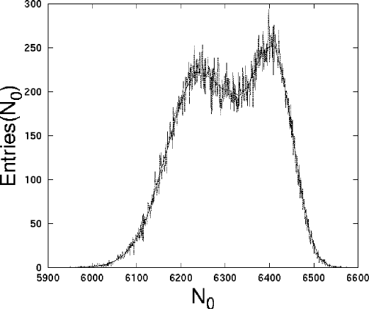
Figure 16.  : The double peak structure at the phase transion point as a function of the the number of vertices, $N_{0}$, for a fixed number of four-simplices, $N_{4}\!=\!32000$.

The effect becomes only apparent for sufficiently large systems (of 32000 and 64000 simplices); for smaller volumes the separation cannot be seen.

From the point of view of quantum gravity, this is of course a disappointing result, because there is no new continuum physics associated with the phase transition. The weakness of the transition could be an indication that a continuous phase transition can be reached by enlarging the space of coupling constants, that is, by extending the action $S_{EH}$. Obvious candidates would be terms containing higher powers of the curvature, which have previously been used in quantum Regge calculus [80].

In both 3d and 4d simplicial gravity, the phases observed on either side of the transition are pathological, in that they do not seem to correspond to an effective quantum geometry of a sensible dimensionality. As already mentioned we find either branched polymers (locally one-dimensional objects) or a condensation of the volume around selected points (yielding an object of arbitrarily large dimension). It is surprising that the rich geometric structure observed in two dimensions has all but disappeared. There are potential cures for this, although there is no guarantee that they will lead to the desired quantum theory.

Within the framework of dynamical triangulations, there are basically two ways of “changing the measure”, in order to improve this state of affairs. One is by using a modified action, but leaving the sum over geometries untouched. Gravity with a squared scalar-curvature term was investigated in [81], but the numerical results indicated that the phase structure remained unchanged. Note that also in $d=2$, the addition of such terms does not change the universality class of pure gravity, as has been shown both numerically (see, for example, [82]) and analytically [83]. The other possibility is to change the sum to a different class of triangulations. A physically motivated example of this kind is the imposition of a causality constraint on Lorentzian geometries. It does lead to a change of universality class in $d=2$, as we have already seen. There are indications that also in $d>2$ a causality condition acts as an effective regulator for the quantum geometry [84]. Numerical investigations of Lorentzian models in higher dimensions are under way.

Another logical possibility is that only the matter-coupled theory possesses a well-defined scaling limit. Recall that in two dimensions, there is a rather narrow window of physically interesting Euclidean continuum theories, namely, Liouville gravity interacting with conformal fields of charge $0\leq c\leq 1$. We simply may have been lucky that pure gravity lies within this range.

Matter interactions could in principle suppress the formation of baby universes in higher dimensions, and the inclusion of gauge (vector) fields was suggested as a promising scenario for testing this conjecture [85]. The simplest model of this kind is the non-compact 4d Abelian gauge model formulated in [75]. Like on a regular lattice, the gauge fields $A_{ij}\equiv-A_{ji}$ are associated with oriented lattice links $\{i,j\}$. A discretized version $P$ of the field strength tensor $F_{\mu\nu}$ can be expressed in terms of “plaquettes” around (oriented) triangles $\{ijk\}$,

$$P_{\{ijk\}}=A_{ij}+A_{jk}+A_{ki}.$$ (136)

The action was taken to be

$$S_{gauge}=\sum_{\{ijk\}}o(\{ijk\})P_{\{ijk\}}^{2},$$ (137)

with $o(\{ijk\})$ denoting the order of the triangle $\{ijk\}$. This factor was included to guarantee that whenever $P^{2}$ is constant for all triangles, $S_{gauge}$ is proportional to the volume $N_{4}$ of the manifold. The action has a simple gauge symmetry and is relatively easy to use in numerical simulations, since it is Gaussian in the vector fields. The number $n_{g}$ of gauge fields can be varied, and for $n_{g}=3$ a new “crinkled” phase with $\gamma_{str}<0$ was observed, replacing the branched-polymer phase. Moreover, the phase transition seemed to be continuous rather than first-order.

However, it was soon realized that this new phase can be obtained in a model without gauge fields, by adding a geometric term

$$S_{\Delta}={n_{g}\over 2}\sum_{\{ijk\}}\log o(\{ijk\})$$ (138)

to the pure-gravity action [76]. Since $S_{\Delta}$ is an ultra-local measure term, one would not really expect it to lead to new continuum physics.

The origin of this term can be traced to a somewhat unfortunate choice of gauge action. At first sight, it seems natural to associate the gauge fields with the links of the triangulation, analogous to what is done on regular, flat lattices. This implies that any charged fields which couple to the gauge fields will be located at the vertices. However, note that scalar fields coupled to gravity in all investigations so far have been placed at the centres of the four-simplexes, to ensure that the number of field degrees of freedom grows proportional to the volume. In the case of fluctuating geometry, this need not be the case if the scalar fields are located at the vertices, since $N_{0}$ may grow much slower than $N_{4}$.

Thus, if our primary aim is to compare the effects of gauge fields on geometry with those of the previously studied scalar fields, the complex-valued charged fields should be associated with the four-simplexes of the triangulation, and the gauge fields with the links of the dual lattice. The pure-gauge action is then a sum over the dual plaquettes, which are the natural duals of the triangles in the original triangulation (see [77] for details).

The two models with the gauge potentials $A$ on the links and on the dual links are dual to each other. The theory defined by (137) (on the triangulation) is equivalent to the gauge theory on the dual lattice, if we add by hand a term (138) to the natural gauge action on the dual lattice [77]. Monte Carlo simulations with gauge fields on the dual links without the term (138), as advocated above, have not detected any effect of the gauge fields on the geometry, in line with previous results for scalar fields and Ising spins coupled to gravity.

Putting a more positive spin on this result, the inclusion of the term (138) is the only example of a modification of the action which has led to a genuine change of the geometry. Although it has no obvious physical interpretation and although the crinkled phase is probably not related to interesting continuum physics, it does give us some hope of finding a physically well-motivated term which does change the geometry in an interesting way, allowing us to define a continuum theory of gravity.

7 Outlook

In these notes we have described in some detail a non-perturbative path-integral approach to quantum gravity, with and without matter. This “dynamical triangulations” method uses an intermediate regularization, in which the space of all space-time geometries is approximated by a set of simplicial complexes with certain edge length assignments, in the spirit of Regge calculus. For a finite volume (that is, for a complex with a finite number of simplices) and fixed space-time topology, this method yields well-defined, convergent partition functions and propagators. The aim in this approach is to understand the critical behaviour of these statistical systems of fluctuating geometry, and investigate their physical properties in the continuum limit, if it exists.

We believe that this ansatz has a number of virtues that make further research worthwhile. Firstly, it works perfectly in two dimensions, leading to a host of analytical and numerical results. There, it agrees with other discrete or continuum formulations, whenever they can be compared, and in some cases turns out to be even more powerful. This gives us considerable confidence in the validity of the method. Moreover, the two-dimensional construction has served as a useful laboratory for defining diffeomorphism-invariant versions of two-point functions and other field-theoretic observables. Dynamical triangulations as a method can be applied in any dimension $d$, but obviously will lead to very different theories, depending on $d$. Only in $d=4$ do we expect to find local, interacting quantum-gravitational degrees of freedom.

Secondly, as has been shown recently, there is also a Lorentzian version of the formulation, where additional causality restrictions are imposed on the space-time geometries, and a well-defined Wick rotation exists. The absence of a natural notion of “analytic continuation” from Euclidean to Lorentzian signature has for a long time stalled progress in discretized path-integral approaches to gravity. Surprisingly, in two space-time dimensions the Euclidean and Lorentzian continuum quantum gravity theories are very different. As a consequence of the causality constraint, the “baby-universe” structure of the Euclidean theory is absent in the Lorentzian sector. This leads to a “smoother” quantum geometry, and well-behaved matter coupling even beyond the $c=1$ barrier. Such a behaviour is very desirable in dimension $d>2$, where so far the dominance of “extreme” geometric phases in Euclidean dynamically triangulated models seems to have prevented the existence of an interesting continuum limit.

In higher dimensions, much work remains to be done to establish whether our method leads to a well-defined continuum quantum theory. In the Euclidean sector, a suitable change of the discretized measure or the inclusion of different types of matter may still lead to long-range correlations. In the Lorentzian sector, there is a genuine chance that the causality restrictions will lead to a qualitatively different phase structure, including a second-order phase transition. The investigation of the Lorentzian models for $d>2$ has only just begun. However, we do not have to start from scratch when trying to solve the theory, but can use the considerable expertise gathered in the Euclidean simulations. Obviously, quantum gravity will not be solved by numerical methods alone, but we have learned from the example of dynamical triangulations in 2d that a mathematically exact analysis and numerical simulations can work hand in hand.

In addition, one can hope for analytical progress in solving the discretized models (which in the case of quantum Regge calculus has always been hampered by the presence of inequalities on the edge lengths, even in $d=2$). In terms of dynamical triangulations, quantum gravity has been turned into a well-defined combinatorial problem, which has already been solved exactly in two dimensions. It is also likely that – analogous to the Euclidean case – mean-field methods can help to elucidate the Lorentzian phase structure in higher dimensions. This may have interesting ramifications for the general study of spaces of pseudo-Riemannian geometries.

In summary, the dynamical-triangulations approach is a promising tool for both analytical and numerical investigations of quantum gravity. It allows for a natural inclusion of matter, and is explicitly reparametrization-invariant. The path integral can be defined for both Euclidean and Lorentzian geometries. In the Lorentzian case, it involves summing over a class of Wick-rotatable space-times with a natural “time”-slicing, reminiscent of the geometric structures appearing in Hamiltonian quantization schemes. We hope that our construction of a Lorentzian path integral will serve as a bridge between the canonical and covariant formulations, benefitting both and improving our understanding of the nature of quantum gravity.