DFTT 73/99

Gauge and gravitational interactions

of non-BPS D-particles

L. Gallot ^a, A. Lerda ^b,a and P. Strigazzi ^a

^a Dipartimento di Fisica Teorica, Università di Torino

and I.N.F.N., Sezione di Torino, Via P. Giuria 1, I-10125 Torino, Italy

^b Dipartimento di Scienze e Tecnologie Avanzate

Università del Piemonte Orientale, I-15100 Alessandria, Italy

We study the gauge and gravitational interactions of the stable non-BPS D-particles of the type I string theory. The gravitational interactions are obtained using the boundary state formalism while the $SO(32)$ gauge interactions are determined by evaluating disk diagrams with suitable insertions of boundary changing (or twist) operators. In particular the gauge coupling of a D-particle is obtained from a disk with two boundary components produced by the insertion of two twist operators. We also compare our results with the amplitudes among the non-BPS states of the heterotic string which are dual to the D-particles. After taking into account the known duality and renormalization effects, we find perfect agreement, thus confirming at a non-BPS level the expectations based on the heterotic/type I duality.

1 Introduction

The spectrum of supersymmetric string theories usually contains a special class of states known as BPS states, which are characterized by the property that their mass is completely determined by their charge under some gauge field. They form short (or ultra short) supersymmetric multiplets and, because of this fact, are stable and protected from quantum radiative corrections. A well-known example of such BPS states is provided by the supersymmetric D$p$-branes of the type II theories (with $p$ even in type IIA and $p$ odd in type IIB) [1]. However, supersymmetric string theories quite often contain states that are stable without being BPS. These are in general the lighest states which carry some conserved quantum numbers. For them there is no particular relation between their mass and their charge; they form long multiplets of the supersymmetry algebra and receive quantum radiative corrections. However, being the lightest states with a given set of conserved quantum numbers, they are stable since they cannot decay into anything else. Usually, it is not difficult to find such non-BPS states with the standard string perturbative methods and analyze their properties at weak coupling; but, since they cannot decay, they should be present also in the strong coupling regime, or equivalently they should appear as non-perturbative (D-brane type) configurations in the weakly coupled dual theory. To verify the existence of these non-BPS states is therefore a very strong test on the duality relations between two string theories which does not rely on supersymmetry arguments. The study of the stable non-BPS D-branes in string theory, pioneered by A. Sen in a remarkable series of papers [2, 3, 4, 5, 6], has attracted a lot of interest during the last year (for reviews see Refs. [7, 8, 9]) also for several other reasons; among them we recall the fact the non-BPS D-branes might be useful for analyzing the non-perturbative properties of the non-supersymmetric field theories that live on their world-volumes, or the fact that they may lead to novel types of relations among string theories [7].

One of the most notable examples of stable non-BPS configurations is provided by the perturbative states at the first excited level of the $SO(32)$ heterotic string [10] which carry the spinor representation of the gauge group and whose mass is given by

$$M_{\rm h}=\frac{2}{\sqrt{\alpha^{\prime}}}=\frac{g_{\rm YM}}{\kappa_{10}}~{}~{}.$$ (1.1)

In the last equality we have introduced the low-energy gauge and gravitational couplings ${g_{\rm YM}}$ and ${\kappa_{10}}$ of the heterotic string following the conventions of Ref. [11] which are also reviewed in Appendix B. Being at the first massive level, these states are non-BPS, but being the lightest ones carrying the spinor representation of $SO(32)$, they are stable and should be present also when one increases the heterotic string coupling constant $g_{\rm h}$. In this process however, the mass $M_{\rm h}$ gets renormalized since there are no constraints on it coming from supersymmetry. Thus we can write

$$M_{\rm h}=\frac{g_{\rm YM}}{\kappa_{10}}~{}f~{}~{},$$ (1.2)

where the renormalization function $f$ can in principle be computed perturbatively in the heterotic string and is such that $f\sim 1$ for $g_{\rm h}\to 0$.

If the heterotic/type I duality [12] is correct, also in the type I theory there should exist stable non-BPS configurations that are spinors of $SO(32)$. Such states do indeed exist and were identified by A. Sen as the non-BPS D-particles of type I [4, 5]; then, an explicit boundary state description for them was provided in Ref. [13] . The mass of these D-particles turns out to be

$$M_{\widetilde{0}}=\frac{1}{\sqrt{\alpha^{\prime}}\,g_{\rm I}}=\frac{g_{\rm YM}}{\kappa_{10}}~{}{2^{-3/4}\,{g_{\rm I}}^{-1/2}}~{}~{},$$ (1.3)

where $g_{\rm I}$, $g_{\rm YM}$ and $\kappa_{10}$ are, respectively, the string, the gauge and the gravitational coupling constants of the type I theory in the conventions of Ref. [11] (see also Appendix B). Comparing Eqs. (1.2) and (1.3), and remembering that under the duality map the heterotic gauge and gravitational couplings turn into the corresponding ones of type I, we can deduce that the renormalization function $f$ must be such that $f\sim{2^{-3/4}\,{g_{\rm I}}^{-1/2}}$ for $g_{\rm I}\to 0$ in order for the masses to agree on both sides. Clearly, this result cannot be obtained using perturbative methods, but is a prediction of the heterotic/type I duality .

In this paper we elaborate further on these stable non-BPS particles and study in detail their gravitational and gauge interactions. On the heterotic side, these can be easily obtained using standard perturbative techniques from correlation functions of vertex operators. In this way one can show, for example, that, at the lowest order in the heterotic string coupling constant, the gravitational and gauge potential energies of two such particles at large distance are given, respectively, by the Newton’s law and the Coulomb’s law for massive and charged point-like objects in ten dimensions. On the type I side, instead, the interactions of the non-BPS D-particles must be obtained using less standard methods and have not been fully investigated so far; indeed, only the general rules for computing string amplitudes with these D-particles have been given in the literature [5, 20]. It is the purpose of this paper to fill this gap.

In particular, we will concentrate on processes involving massless string modes that are responsible for the long range interactions among D-particles. To study the gravitational interactions we adopt the boundary state formalism [21, 22, 23] and obtain the energy due to the exchange of closed string states between two D-particles by simply computing the diffusion amplitude between the two corresponding boundary states in relative motion [24, 25] (for recent reviews on the boundary state formalism and its applications see Ref. [26]). Then, by taking the large distance limit to which only graviton and dilaton exchanges contribute, we find that the gravitational potential energy of two D-particles exactly agrees with the one of their heterotic duals, provided that the duality relations and the mass renormalization previously discussed are taken into account.

For the gauge interactions, instead, the situation is a bit more involved. In fact, we cannot use any more the boundary state formalism since this accounts only for the couplings of the D-particles with the closed strings that live in the bulk, but is completely blind to the other bulk sector of the type I theory consisting of open strings with Neumann boundary conditions in all directions to which the $SO(32)$ gauge fields belong. On the other hand, the open strings attached to the D-particles have Neumann boundary conditions only along the time direction. Therefore, to study the gauge interactions of our D-particles we should consider scattering amplitudes involving open strings with mixed boundary conditions in an odd number of dimensions. Calculations of open string amplitudes with mixed boundary conditions have already appeared in the analyses of systems of several D-branes with different dimensionality (see for instance Ref. [27]), and require the use of twist operators to produce mixed boundary conditions in certain directions. These twist operators were used in the past to study strings on orbifolds [28], and have been recently reconsidered from an abstract conformal field theory point of view [29]. Using such twist operators and applying the rules of Refs. [5, 20], we will describe how to compute scattering amplitudes involving non-BPS D-particles and bulk open strings of type I. Special care is required in these calculations because the twist operators that we use change the boundary conditions in an odd number of directions. In particular, we will explicitly determine the gauge coupling of the D-particles by evaluating a correlation function on a disk with two boundary components produced by the insertion of two twist operators. The result of this calculation is extremely simple, namely the non-BPS D-particles couple minimally to the gauge field. Exploiting this fact, we then determine the gauge potential energy of a pair of D-particles at large distance and see that after taking into account the duality map, this exactly agrees with the corresponding energy computed in the heterotic theory.

This paper is organized as follows: in Section 2 we compute the gauge coupling of a non-BPS D-particle of type I by evaluating a disk diagram with two twist insertions, and then determine the gauge potential energy between two D-particles. In Section 3 we use the boundary state formalism to compute the gravitational contribution to the potential energy of two (moving) D-particles. In Section 4 we study the gauge and gravitational interactions of the non-BPS heterotic states that are dual to the D-particles. In Section 5 we compare the results for the non-BPS D-particles and for their dual heterotic states, and discuss their relations. In Appendix A we show how to compute the gauge interactions between two BPS D-strings of type I by extending the method of Section 2 and verify the no-force condition. Finally, Appendices B and C contain our conventions and a list of more technical formulas.

2 Type I D-particle interactions: the gauge amplitude

As we mentioned in the introduction, an important check of the heterotic/type I duality has been the discovery by A. Sen [3, 4, 5] that the stable non-BPS heterotic states carrying the spinor representation of $SO(32)$ at the first massive level are dual to the non-BPS D-particles of type I. Specific rules for computing amplitudes involving such D-particles have been given by A. Sen [5] and E. Witten [20] in two different ways which we briefly recall here. Sen’s approach heavily relies of the use of Chan-Paton factors to distinguish the various kinds of open strings. The 0-0 strings, whose end-points lie on the non-BPS D-particle, contain both states that are even and states that are odd under $(-1)^{F}$; the former carry a Chan-Paton factor 1l, the latter a Chan-Paton factor $\sigma_{1}$. The 9-0 strings stretching between one of the 32 D9 branes of the type I background and a D-particle contain only $(-1)^{F}$ even states but, due to the existence of an odd number of fermionic zero modes, their vertex operators comprise the standard GSO-even part as well as the corresponding GSO-odd part, weighted by Chan-Paton factors $\left(\begin{array}[]{c}1\\ 0\end{array}\right)$ and $\left(\begin{array}[]{c}0\\ 1\end{array}\right)$ respectively. Besides these factors, the 9-0 strings also carry a Chan-Paton factor $\lambda^{A}$ ($A=1,\dots,32$) labeling the fundamental representation of the $SO(32)$ gauge group. Finally, the 9-9 strings are the usual open strings of the type I theory which are GSO projected and carry only the standard Chan-Paton factors of the gauge group.

The presence of the unusual Chan-Paton factors 1l, $\sigma_{1}$, $\left(\begin{array}[]{c}1\\ 0\end{array}\right)$ or $\left(\begin{array}[]{c}0\\ 1\end{array}\right)$ shows that the states of the 0-0 and 9-0 sectors have a non trivial structure which is really due to the presence of an odd number of fermionic zero modes. In order to remedy to this oddity, in Ref. [20] Witten has proposed to introduce an extra one-dimensional fermion $\eta$ on each boundary of the string world-sheet lying on a D-particle. In this way, in the 9-0 sector one recovers an even number of fermionic zero modes and can perform the usual GSO projection. Also in the 0-0 sector one performs a (generalized) GSO projection to obtain physical states, but since the extra fermion $\eta$ is odd under this GSO parity, one obtains two types of 0-0 states, similarly to what found by Sen.

Let us now give some details on how to construct the massless states in the various open string sectors using Witten’s rules. We start with the NS sector of the 0-0 strings where at the massless level there are nine scalars $x^{i}$ ($i=1,\dots,9$) corresponding to the freedom of moving the D-particle in its nine tranverse directions. These modes, which are present also on the BPS D0 brane of the type IIA theory, correspond to vertex operators ${\cal V}_{x^{i}}$ that do not depend on the boundary fermion $\eta$. In the $(-1)$ superghost picture, these vertex operators are simply

$${\cal V}_{x^{i}}^{(-1)}=\psi^{i}~{}{\rm e}^{-\phi}~{}~{}.$$ (2.1)

Notice that there is no factor of ${\rm e}^{{\rm i}k\cdot X}$ in (2.1) because massless states of $0$-$p$ strings have no momentum. Let us now consider the R sector of the 0-0 strings. Here both the ten world-sheet fermions $\psi^{\mu}$ and the boundary fermion $\eta$ possess zero modes so that the massless R states form a GSO-even spinor $\xi^{\alpha}$ of $SO(1,10)$. Note that in this case the GSO projection is simply the ten-dimensional chirality projection which is natural when one extends $SO(1,9)$ to $SO(1,10)$ by adding $\eta$. Thus, in the $(-1/2)$ superghost picture the vertex operator for the massless R states reads

$${\cal V}_{\xi^{\alpha}}^{(-1/2)}={1+\eta\over 2}\,S^{\alpha}~{}{\rm e}^{-\phi/2}$$ (2.2)

where $S^{\alpha}$ is the spin field of conformal dimension $10/16$ associated to the ten world-sheet fermions. Upon quantization, the $16$ massless fermionic modes described by (2.2) account for the $2^{16/2}=256$ degeneracy of the non-BPS D-particle.

We now turn to the 9-0 strings which are more relevant for our purposes. Since the NS sector does not contain massless states, we just consider the R sector. In this case, the only world sheet fermion to have a zero mode is $\psi^{0}$ so that the ground state is a GSO-even (chiral) spinor of the algebra $SO(1,1)$ generated by $\psi^{0}_{0}$ and $\eta$. Hence, the vertex operator describing the massless modes of the 9-0 sector should contain

• a spin field $S$ associated to the fermion $\psi^{0}$, of conformal dimension 1/16;

• a boundary changing operator $\Delta$ for the nine space directions transverse to the D-particle, of conformal dimension 9/16;

• a GSO (or chirality) projector for the Clifford algebra of $SO(1,1)$ ${1+\psi_{0}^{0}\eta\over 2}$, of conformal dimension zero;

• a superghost contribution in the $-1/2$ picture ${\rm e}^{-\phi/2}$, of conformal dimension 3/8;

• a gauge Chan-Paton factor $\lambda^{A}$ to specify which of the 32 D9 branes one is considering.

Thus, we have

$${\cal V}_{90}^{(-1/2)}=\lambda^{A}~{}{1+\psi_{0}^{0}\,\eta\over 2}~{}S~{}\Delta~{}{\rm e}^{-\phi/2}~{}~{}.$$ (2.3)

It is easy to check that the operator (2.3) has indeed conformal dimension 1 as it should be for a physical vertex operator. Notice that the GSO projection in (2.3) keeps only one fermionic degree of freedom for each value of the index $A$ of the fundamental representation of $SO(32)$. Upon quantization, the states described by ${\cal V}_{90}$ form a spinorial representation of $SO(32)$, and hence we can conclude that the marginal operator (2.3) accounts for the $SO(32)$ degeneracy of the non-BPS D-particle. Since in type I the strings are unoriented, we should consider also the 0-9 sector. This is merely related to the 9-0 sector through the action of the world-sheet parity $\Omega$. Recalling that $\Omega$ simply acts by transposition on the Chan-Paton factors without changing the physical content of the vertex operators, we have

$${\cal V}_{09}^{(-1/2)}=\Omega~{}{\cal V}_{90}^{(-1/2)}={\lambda^{t}}^{\,A}~{}{1+\psi_{0}^{0}\,\eta\over 2}~{}S~{}\Delta~{}{\rm e}^{-\phi/2}~{}~{}.$$ (2.4)

Notice in particular that the $SO(1,1)$ GSO projection is the same in both vertices (2.3) and (2.4).

Finally, there are the 9-9 strings which, as we mentioned above, are the usual open strings of the type I theory; in particular in the NS sector at the massless level we find the $SO(32)$ gauge bosons which are described by the following vertex operators in the $(-1)$ superghost picture

$${\cal V}_{\rm gauge}^{(-1)}=\Lambda^{AB}~{}A_{\mu}\,\psi^{\mu}~{}{\rm e}^{{\rm i}k\cdot X}~{}{\rm e}^{-\phi}~{}~{},$$ (2.5)

where $\Lambda^{AB}$ are the generators of $SO(32)$ in the fundamental representation (see Appendix B for our conventions) and $A_{\mu}$ is the polarization vector.

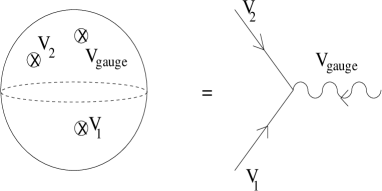
We now face the problem of finding the coupling between the non-BPS D-particle and the gauge field. Since the latter belongs to the 9-9 massless sector, the diagram we have to compute corresponds to a disk with a part of its boundary on the D-particle and a part on the D9-branes from which the gauge boson is emitted. This is represented in the Figure 1.

Figure 1: The disk diagram describing the gauge coupling of a type I D–particle

We thus have to insert two vertices containing the boundary changing operator $\Delta$ which turns a boundary of type 0 into one of type 9 (or viceversa). The obvious choice is then to make insertions of the vertices ${\cal V}_{90}$ and ${\cal V}_{09}$ given in (2.3) and (2.4) which correspond to the $SO(32)$ degeneracy of the D-particle. Note that, although no momentum is carried by these vertices, the emitted gauge boson may have non-zero space momentum. Indeed, the twist operators $\Delta$ are reservoirs of transverse momentum [28] which allow emissions with non-zero momentum in the transverse directions; on the other hand, this is to be expected because the presence of a D-brane breaks the translational invariance in transverse space. Note also that, due to the insertion of the two vertices ${\cal V}_{90}$ and ${\cal V}_{09}$, the boundary component associated with the D-particle carries indices in the bi-fundamental representation of $SO(32)$. This is consistent with the fact that a D-particle should emit all, both massless and massive, perturbative open string states which group in the adjoint or in the symmetric representation of $SO(32)$.

The gauge coupling of a (static) D-particle is then given by the expectation value of the gauge boson emission vertex (2.5) in the “vacuum” representing the D-particle. Thus, the diagram of Figure 1 corresponds to

$${\cal F}^{\rm gauge}=\langle\Omega_{09}|\,{\cal V}^{(-1)}_{\rm gauge}|\,\Omega_{90}\rangle$$ (2.6)

where

$$|\Omega_{90}\rangle=\lim_{z\rightarrow 0}{\cal V}^{(-1/2)}_{09}(z)\,|0\rangle~{}~{}~{}{\rm and}~{}~{}~{}\langle\Omega_{09}|=\lim_{z\rightarrow\infty}\langle{0}|\,{\cal V}^{(-1/2)}_{09}(z)~{}~{}.$$ (2.7)

Note that due to the presence of the twist operators in ${{\cal V}}_{09}$ and ${{\cal V}}_{90}$, the expectation value of the gauge emission vertex is not vanishing, as we will explicitly see in the following.

After including the normalization factor ${\cal C}_{\rm disk}$ appropriate of any disk amplitude, the normalization factors ${\cal N}_{\rm R}$ for the R vertices (2.3) and (2.4), and ${\cal N}_{\rm NS}$ for the NS vertex (2.5) , ${\cal F}^{\rm gauge}$ may be reexpressed as a 3-point function on the world sheet and reads

$${\cal F}^{\rm gauge}={\cal C}_{\rm disk}~{}{\cal N}^{2}_{\rm R}~{}{\cal N}_{\rm NS}~{}\int d\mu(z_{i})~{}\left\langle c\,{\cal V}^{(-1/2)}_{09}(z_{1})~{}c\,{\cal V}^{(-1)}_{\rm gauge}(z_{2})~{}c\,{\cal V}^{(-1/2)}_{90}(z_{3})\right\rangle_{\eta}~{}~{}.$$ (2.8)

where we have also added a ghost $c$ in each vertex operator. The notation $\langle~{}\rangle_{\eta}$ means that the correlator must be evaluated by including the action for the boundary fermion $\eta$ as explained in Ref. [20].

The correlation function in (2.8) may be decomposed into a longitudinal and a transverse piece. The latter vanishes because

$$\Big{\langle}\Delta(z_{1})~{}\psi^{i}(z_{2})~{}{\rm e}^{{\rm i}k\cdot X(z_{2})}~{}\Delta(z_{3})\Big{\rangle}=0$$ (2.9)

for $i=1,\ldots,9.$ Thus, there is no emission of gauge bosons with polarization $A_{i}$ along the transverse directions, as it should be for a minimally coupled particle at rest. We then consider the longitudinal part for which the basic correlators are

$$\Big{\langle}c(z_{1})\,c(z_{2})\,c(z_{3})\Big{\rangle} = z_{12}\,z_{13}\,z_{23}~{}~{},$$ (2.10)

$$\Big{\langle}{\rm e}^{-\phi(z_{1})/2}\,{\rm e}^{-\phi(z_{2})}\,{\rm e}^{-\phi(z_{3})/2}\Big{\rangle} = z_{12}^{-1/2}\,z_{13}^{-1/4}\,z_{23}^{-1/2}~{}~{},$$ (2.11)

$$\Big{\langle}\Delta(z_{1})\,{\rm e}^{{\rm i}k\cdot X(z_{2})}\,\Delta(z_{3})\Big{\rangle} = z_{12}^{-\alpha^{\prime}k^{2}}\,z_{13}^{\alpha^{\prime}k^{2}-9/8}\,z_{23}^{-\alpha^{\prime}k^{2}}~{}~{}.$$ (2.12)

Notice that in (2.12) the transverse momentum $k^{i}$ of the emitted gauge boson is not subject to any constraint, as we have anticipated. The remaining correlator to be considered is

$$\Big{\langle}\left({1+\psi^{0}_{0}\,\eta\over 2}S(z_{1})\right)~{}\psi^{0}(z_{2})~{}\left({1+\psi^{0}_{0}\,\eta\over 2}S(z_{3})\right)\Big{\rangle}_{\eta}~{}~{}.$$ (2.13)

This splits into four pieces, two of which vanish. Indeed, according to Ref. [20] the only non-vanishing correlation functions are those containing one factor of $\eta$. In particular one has

$$\Big{\langle}\eta\Big{\rangle}_{\eta}=\sqrt{2}~{}~{}~{},~{}~{}~{}\Big{\langle}1\Big{\rangle}_{\eta}=0~{}~{}.$$ (2.14)

Finally, we have

$$\Big{\langle}\psi^{0}_{0}S(z_{1})~{}\psi^{0}(z_{2})~{}S(z_{3})\Big{\rangle}=\Big{\langle}S(z_{1})~{}\psi^{0}(z_{2})~{}\psi^{0}_{0}S(z_{3})\Big{\rangle}=z_{12}^{-1/2}\,z_{13}^{3/8}\,z_{23}^{-1/2}~{}~{}.$$ (2.15)

Notice that a correlation function similar to (2.15) appears in the 2D Ising model. Indeed, the spin field $S$ may be identified with the order parameter $\sigma$ (i.e. the magnetization) while the other spin field $\psi^{0}_{0}S$ plays the role of the disorder parameter $\mu$ [31].

Inserting Eqs. (2.10)-(2.15) into (2.8) and exploiting the projective invariance to fix the position of the three punctures at arbitrary values, we easily get

$${\cal F}^{\rm gauge} = -\,{{\cal C}_{\rm disk}\,{\cal N}_{\rm R}^{2}\,{\cal N}_{\rm NS}\over\sqrt{2}}~{}{\rm Tr}({\lambda^{t}}^{A}\,\Lambda^{BC}\,\lambda^{D})~{}A_{0}~{}\int d\mu(z_{i})~{}\left({z_{13}\over z_{12}z_{23}}\right)^{\alpha^{\prime}k^{2}}$$ (2.16)

$$= -\,{{\cal C}_{\rm disk}\,{\cal N}_{\rm R}^{2}\,{\cal N}_{\rm NS}\over\sqrt{2}}~{}{\rm Tr}({\lambda^{t}}^{A}\,\Lambda^{BC}\,\lambda^{D})~{}A_{0}~{}~{}.$$

Then, using the explicit expressions of the normalization coefficients and Chan-Paton factors given in Appendix B, we can rewrite ${\cal F}^{\rm gauge}$ as follows

$${\cal F}^{\rm gauge}=-\,{\rm i}~{}{g_{\rm YM}\over\sqrt{2}}~{}\left(\delta^{AB}\,\delta^{CD}-\delta^{AC}\,\delta^{BD}\right)~{}A_{0}~{}~{},$$ (2.17)

where $g_{\rm YM}$ is the gauge coupling constant of the type I theory.

Eq. (2.17) represents the amplitude for the emission of a gauge boson with longitudinal polarization $\xi_{0}$ and color index $(BC)$ from a 0-boundary in the bi-fundamental of $SO(32)$. The appearance of this representation is a direct consequence of our construction in which the D-particle is represented by the 0-component of a disk boundary produced by the insertion of the vertex operators ${\cal V}_{90}$ and ${\cal V}_{09}$. On the other hand, the $SO(32)$ spinor degeneracy of the non-BPS D-particle of type I arises from the (second) quantization of the 32 massless fermionic zero-modes of the 0-9 open strings, and thus it is clear that such a degeneracy cannot be seen in our operator formalism. This fact should not be surprising because a completely analogous situation occurs in the familiar description of D$p$-branes using boundary states. Indeed, a boundary state is a single state that correctly represents a D$p$-brane and its couplings to the bulk closed strings, even if it does not account for the degeneracy of the D$p$-brane under the supersymmetry algebra. Similarly, in our case the 0-component of the disk boundary produced by the insertion of ${\cal V}_{90}$ and ${\cal V}_{09}$ correctly describes a D-particle and allows to obtain its coupling with the bulk 9-9 open strings, even if does not account for its degeneracy under the gauge group. In fact, as we will see later and in the following sections, using this construction we are able to obtain non trivial information about the gauge interactions between two D-particles at large distance. Moreover, after taking into account the known duality relations, we will show that the results obtained in this way exactly agree with those in the heteroric theory, as required by the heterotic/type I duality, thus confirming the validity of our construction.

Using the result (2.17) we can now easily compute the gauge potential energy ${V}_{\rm I}^{\rm gauge}$ due to the exchange of the $SO(32)$ gauge bosons between two D-particles. As indicated in Figure 2,

Figure 2: The diagram describing the gauge amplitude between two D-particles

this can be obtained simply by sewing two emission amplitudes ${\cal F}^{\rm gauge}$ with the gauge boson propagator

$${\cal P}={\eta^{\alpha\beta}\over q^{2}}~{}\left(\delta^{BB^{\prime}}\delta^{CC^{\prime}}-\delta^{BC^{\prime}}\delta^{CB^{\prime}}\right)~{}~{},$$ (2.18)

yielding

$${V}_{\rm I}^{\rm gauge}=-\,\frac{g_{\rm YM}^{2}}{2}~{}\left(\delta^{AE}\,\delta^{FD}-\delta^{AF}\,\delta^{DE}\right)~{}\frac{1}{q^{2}}~{}~{}.$$ (2.19)

Performing a Fourier transform, we get the following (static) gauge potential in configuration space

$${V}_{\rm I}^{\rm gauge}(r)=-\,\frac{g_{\rm YM}^{2}}{2}~{}\left(\delta^{AE}\,\delta^{FD}-\delta^{AF}\,\delta^{DE}\right)~{}\frac{1}{7\,\Omega_{8}\,r^{7}}~{}~{},$$ (2.20)

where $\Omega_{q}=2\pi^{(q+1)/2}/\Gamma((q+1)/2)$ is the area of a unit $q$-dimensional sphere. Eq. (2.20) clearly represents a “Coulomb-like” potential energy for point particles at a distance $r$ in ten dimensions.

We conclude this section by mentioning that the same results (2.17) and (2.20) can be obtained also using the rules given by A. Sen in Ref. [5] for computing amplitudes with non-BPS D-particles.

3 Type I D-particle interactions: the gravitatio- nal amplitude

The gravitational contribution to the scattering of two non-BPS D-particles of type I can be calculated, at the leading order in the string coupling constant, from the diffusion amplitude between two corresponding boundary states. The boundary state description of the non-BPS D-particles has already been given in Refs. [5, 13] from which we recall the results that are relevant in the forthcoming analysis. For details and conventions on boundary states, we refer the reader to Refs. [23, 25, 13].

In the closed string operator formalism, one describes a D$p$-brane by means of a boundary state $|{Dp}\rangle$ [21, 22]. This is a closed string state which inserts a boundary on the world-sheet, enforces on it the appropriate boundary conditions and represents the source for the closed strings emitted by the brane. As an example, the boundary state for a BPS D-particle of type IIA may formally be written as 

$$|{D0}\rangle_{\rm{IIA}}=|{D0}\rangle_{{\rm NS}}+|{D0}\rangle_{{\rm R}}~{}~{},$$ (3.1)

where the NS-NS and the R-R components are both proportional to $T_{0}$ which is the tension of the D-particle in units of the gravitational coupling constant, namely

$$T_{0}=8\,\pi^{7/2}\,\alpha^{\prime\,3/2}~{}~{}.$$ (3.2)

The presence of both the NS-NS and the R-R components implies that the spectrum of the open strings living on the D-particle is GSO-projected. The partition function of such open strings may be obtained by evaluating the cylinder/annulus amplitude in the closed string channel which is given by

$${}_{\rm{IIA}}\langle{D0}|P|{D0}\rangle_{\rm{II}A}~{}~{},$$ (3.3)

and then performing a modular transformation. In Eq. (3.3), $P$ denotes the closed string propagator

$$P={\alpha^{\prime}\over 2}\,{1\over L_{0}+\widetilde{L}_{0}-a-\widetilde{a}}~{}~{}.$$ (3.4)

where $a$ ($\widetilde{a}$) is the left (right) intercept ($a_{{\rm NS}}=1/2$, $a_{{\rm R}}=0$).

The boundary state for the non-BPS D-particle of the IIB theory [3, 13] has instead only a component along the NS-NS sector and a tension $T_{\widetilde{0}}$ greater by a factor of $\sqrt{2}$ than $T_{0}$. Thus, we can write

$$|{D\widetilde{0}}\rangle_{\rm{IIB}}=\sqrt{2}|{D0}\rangle_{{\rm NS}}~{}~{}.$$ (3.5)

As a consequence, there is no GSO-projection in the spectrum of the open strings lying on the non-BPS D-particle and the presence of a tachyon in the NS sector renders it unstable. However, if we consider the type I theory [32], the tachyon is removed by the projection onto states invariant under the world-sheet parity $\Omega$ [3, 13]. In the boundary state formalism, the $\Omega$ projection is implemented by adding the so-called crosscap state $|{C}\rangle$ [22], which corresponds to inserting on the closed string world-sheet a boundary with opposite points identified. The negative $(-32)$ charge for the non-propagating R-R 10-form that the crosscap generates in the background, must be canceled by the introduction of 32 D9-branes. Hence, the type I theory possesses a background “boundary state” given by [22]

$${1\over\sqrt{2}}\Big{(}|{C}\rangle+32|{D9}\rangle\Big{)}$$ (3.6)

where the factor of $1/\sqrt{2}$ has been introduced to obtain the right normalization of the various spectra. Then, the partition function for unoriented open 9-9 strings, given by the sum of the annulus and the Möbius strip contributions, is

$${1\over 2}\left(2^{10}\langle{D9}|P|{D9}\rangle+2^{5}\langle{D9}|P|{C}\rangle+2^{5}\langle{C}|P|{D9}\rangle\right)~{}~{},$$ (3.7)

while the contribution of the Klein bottle

$${1\over 2}\langle{C}|P|{C}\rangle$$ (3.8)

added to the torus contribution gives the partition function for unoriented closed strings.

The boundary state of the non BPS D-particle of type I reads

$$|{D\widetilde{0}}\rangle_{I}={1\over\sqrt{2}}\left(\sqrt{2}|{D0}\rangle_{{\rm NS}}\right)=|{D0}\rangle_{{\rm NS}}$$ (3.9)

where we have added the same factor of $1/\sqrt{2}$ for consistency with (3.6). The mass of the D-particle is then given by

$$M_{\widetilde{0}}=\frac{1}{\sqrt{2}}\,{T_{\widetilde{0}}\over\kappa_{10}}={T_{0}\over\kappa_{10}}={1\over\sqrt{\alpha^{\prime}}\,g_{I}}$$ (3.10)

where $\kappa_{10}$ is the ten dimensional gravitational coupling constant of the type I theory (see Appendix B). The partition function for open 0-0 strings living on the D-particle, obtained by summing the contributions from the annulus and the Möbius strip, is

$${}_{{\rm NS}}\langle{D0}|P|{D0}\rangle_{{\rm NS}}+{1\over 2}\Big{(}\sqrt{2}\,\langle{C}|P|{D0}\rangle_{{\rm NS}}+\sqrt{2}~{}{}_{{\rm NS}}\langle{D0}|P|{C}\rangle\Big{)}~{}~{}.$$ (3.11)

In this theory, there are also 0-9 and 9-0 open strings with one end on the D-particle and the other on one of the 32 D9 branes of the type I background. The world-sheet parity $\Omega$ exchanges the two sectors 0-9 and 9-0 so that we only retain symmetric combinations corresponding to the partition function

$${32\sqrt{2}\over 2}\Big{(}{}_{{\rm NS}}\langle{D0}|P|{D9}\rangle+\langle{D9}|P|{D0}\rangle_{{\rm NS}}\Big{)}~{}~{}.$$ (3.12)

The spectrum of open strings stretching between two different (distant) D-particles at rest, one labeled with a prime, has a partition function given by

$${1\over 2}\left((\sqrt{2})^{2}{}_{{\rm NS}}\langle{D0}|P|{D0^{\prime}}\rangle_{{\rm NS}}+(\sqrt{2})^{2}{}_{{\rm NS}}\langle{D0^{\prime}}|P|{D0}\rangle_{{\rm NS}}\right)$$ (3.13)

where the factor of one-half indicates that, compared to the IIB case, only the $\Omega$ symmetric combinations are retained. Notice that, at sufficiently small distance, a tachyon develops in this open string spectrum signaling the instability of the configuration which decays into the vacuum [5].

Our aim is to study the diffusion of a moving D-particle with a velocity $v$ along one space direction, say $X^{1}$, on another D-particle at rest at the origin. Such an interaction may be evaluated analyzing the spectrum of the open strings stretching between the two objects with modified boundary conditions in the 0 and 1 directions. This can be done generalizing the treatment for the BPS D-branes presented in Ref. [33], but we find it simpler to use the method of the boosted boundary state [24, 25]. Indeed, the interaction amplitude just reads

$${\cal A}_{\rm I}(v)={}_{{\rm NS}}\langle{D0^{\prime}}|P\,\Lambda|{D0}\rangle_{{\rm NS}}+{}_{{\rm NS}}\langle{D0}|\Lambda^{\dagger}\,P|{D0^{\prime}}\rangle_{{\rm NS}}$$ (3.14)

where $\Lambda$ is the boost operator

$$\Lambda={\rm e}^{{\rm i}\pi\nu J^{01}}$$ (3.15)

acting on the boundary state of a particle at rest. Here we have $v=\rm{th}(\pi\nu)$ and $J^{\mu\nu}$ is the generator of the Lorentz transformations. Notice that the amplitude (3.14) reduces to the static one (3.13) in the limit of vanishing velocity. The boosted boundary state reads

$$\Lambda|{D0,\pm}\rangle_{{\rm NS}} = \frac{T_{0}}{2}\,{1\over\gamma}\,\delta^{(8)}(x)\,\delta(x^{0}\,v+x^{1})\,\exp\left[-\sum_{n=1}^{\infty}a_{n}^{\dagger}\cdot S\cdot\widetilde{a}_{n}^{\dagger}\right]$$ (3.16)

$$\times\,\exp\left[\pm\,{\rm i}\sum_{r=\frac{1}{2}}^{\infty}\psi_{r}^{\dagger}\cdot S\cdot\widetilde{\psi}_{r}^{\dagger}\right]\prod_{\mu=0}^{9}|{k^{\mu}=0}\rangle$$

where the boundary conditions are encoded in the matrix $S=(-{\cal V}_{01},-{\hbox{ 1\kern-2.27621ptl}}_{8})$ with

$${\cal V}_{01}=\left(\begin{array}[]{cc}\cosh(2\pi\nu)&\sinh(2\pi\nu)\\ \sinh(2\pi\nu)&\cosh(2\pi\nu)\\ \end{array}\right)~{}~{}.$$ (3.19)

Note that $\cosh(\pi\nu)\equiv\gamma$ is the Lorentz factor.

The interaction amplitude ${\cal A}_{\rm I}(v)$ can be evaluated using standard techniques [24, 25] and explicitly reads

$${\cal A}_{\rm I}(v) = (8\pi^{2}\alpha^{\prime})^{-\frac{1}{2}}\,\int_{-\infty}^{\infty}d\tau\int_{0}^{\infty}ds\,\,s^{-\frac{9}{2}}\,\,{\rm e}^{-{b^{2}+\tau^{2}v^{2}\gamma^{2}\over 2\pi\alpha^{\prime}s}}$$ (3.20)

$$\,2\,\sinh(\pi\nu)\left[{f_{3}^{6}(q)\,\theta_{3}(-{\rm i}\nu|{\rm i}s)-f_{4}^{6}(q)\,\theta_{4}(-{\rm i}\nu|{\rm i}s)\over f_{1}^{6}(q)\,\theta_{1}(-{\rm i}\nu|{\rm i}s)}\right]$$

in which $q={\rm e}^{-\pi s}$, $\tau$ is the proper time of the moving particle and $b$ is the impact parameter. We are now in a position to extract the long range interaction potential energy $V_{\rm I}^{\rm grav}$ due to gravitational exchange between the two particles. To do so we have to perform the limit $s\rightarrow\infty$ in the integrand of Eq. (3.20), then integrate on the variable $s$ and finally identify the potential energy according to

$${\cal A}_{\rm I}(v)=\int_{-\infty}^{\infty}d\tau\,\,V_{\rm I}^{\rm grav}~{}~{}.$$ (3.21)

In the non relativistic limit, we obtain the Newton’s law with its first correction

$$V_{\rm I}^{\rm grav}(r)=(2\kappa_{10})^{2}\,{M_{\widetilde{0}}^{2}\over 7\,\Omega_{8}\,r^{7}}\left(1+\frac{1}{2}\,v^{2}\right)+o(v^{2})\qquad v\rightarrow 0$$ (3.22)

where we have introduced the radial coordinate $r^{2}=b^{2}+v^{2}\gamma^{2}\tau^{2}$. Thus, in the non relativistic limit the boundary state calculation reproduces correctly the gravitational potential energy that we expect for a pair of D-particles in relative motion.

4 Interactions of the heterotic non-BPS states

The non-BPS D-particles described in the previous sections account for the presence in the spectrum of the type I theory of long super-multiplets of states carrying the spinorial representation of $SO(32)$. These non-perturbative states are dual to those appearing at the first massive level in the heterotic theory. Carrying the same quantum numbers, one naturally expects that these heterotic states have the same kind of interactions as the D-particles of type I. In this section we will check this idea and investigate the gauge and gravitational interactions of the non-BPS heterotic states using standard tools of perturbative string theory. In doing so, we will adopt the bosonized formulation of the heterotic string in which the gauge degrees of freedom are described by sixteen chiral bosons ${\widetilde{X}}^{I}$ ($I=1,\cdots,16$) appropriately compactified [10].

The long super-multiplet of the stable heterotic states appears at the first massive level $\Big{(}M_{\rm h}^{2}=4/\alpha^{\prime}\Big{)}$, and contains the following bosonic states

$$\psi_{-3/2}^{\mu}|{k}\rangle\otimes|{K^{I}}\rangle~{}~{}~{} ~{}~{}~{}\alpha_{-1}^{(\mu}\psi_{-1/2}^{\nu)}|{k}\rangle\otimes|{K^{I}}\rangle~{}~{},$$ , (4.1)

$$\alpha_{-1}^{[\mu}\psi_{-1/2}^{\nu]}|{k}\rangle\otimes|{K^{I}}\rangle~{}~{}~{} ~{}~{}~{}\psi_{-1/2}^{\mu}\psi_{-1/2}^{\nu}\psi_{-1/2}^{\rho}|{k}\rangle\otimes|{K^{I}}\rangle~{}~{}.$$ , (4.2)

with $\mu,\nu,...=0,\ldots,9$. In these formulas $k$ denotes the space-time momentum ($k^{2}=-M_{\rm h}^{2}$) while $K^{I}$ is the adimensional momentum associated to the sixteen internal coordinates ${\widetilde{X}}^{I}$. The states of Eq. (4.1) describe massive degrees of freedom which transform in the 44 representation of the Lorentz group, whereas those of Eq. (4.2) transform in the 84 . The level matching condition requires that $K^{2}=4$. This may be realized for example by taking $K^{I}$ to be of the form $(\pm{1\over 2},\pm{1\over 2},,\cdots,\pm{1\over 2})$ with an even number of $+$ signs, thus obtaining the spinorial representation of $SO(32)$ with positive chirality. The vertex operators for the states (4.1) and (4.2) will be denoted by $\cal V$ and can be found in Appendix C both in the $(-1)$ and in the $(0)$ superghost pictures.

We now study the interactions of these states with the massless gauge bosons of $SO(32)$. In the bosonized formulation of the heterotic string we must distinguish between the states associated to the $16$ Cartan generators that are given by

$$A_{\mu}\,\psi_{-1/2}^{\mu}|{q}\rangle\otimes\widetilde{\alpha}_{-1}^{I}|{Q=0}\rangle\quad\mbox{with}~{}~{}q^{2}=0\quad\mbox{and}~{}~{}I=1,\ldots,16~{}~{},$$ (4.3)

and those associated to the remaining $480$ generators which are instead given by

$$A_{\mu}\,\psi_{-1/2}^{\mu}|{q}\rangle\otimes|{Q}\rangle\quad\mbox{with}~{}~{}q^{2}=0$$ (4.4)

and the internal momentum $Q$ of the form $(0,\cdots,0,\pm 1,0,\cdots,0,\pm 1,0,\cdots,0)$. Also the vertex operators for the states (4.3) and (4.4), which we denote collectively by ${\cal V}_{\rm gauge}$, can be found in Appendix C in the $(-1)$ and $(0)$ superghost pictures.

The gauge coupling of the states (4.1) and (4.2) is obtained by simply computing the 3-point function on the sphere among two vertex operators ${\cal V}$ and one vertex operator ${\cal V}_{\rm gauge}$ (see Figure 3).

Figure 3: The 3-point function on the sphere

Including the normalization factor ${\cal C}_{0}$ appropriate of any tree-level closed string amplitude and a normalization factor $\widehat{{\cal N}}$ for each vertex operator, we have

$$\Big{(}{\cal F}_{3}^{\rm gauge}\Big{)}_{\alpha_{1}\alpha_{2}}={\cal C}_{0}\,\widehat{{\cal N}}^{3}\int d^{2}\mu(z_{i},\bar{z}_{i})\,\Big{\langle}c{\bar{c}}{\cal V}^{(-1)}_{1}(z_{1},\bar{z}_{1})\,c{\bar{c}}{\cal V}^{(-1)}_{2}(z_{2},\bar{z}_{2})\,c{\bar{c}}{\cal V}^{(0)}_{\rm gauge}(z_{3},\bar{z}_{3})\Big{\rangle}$$ (4.5)

where $\alpha_{1}$ and $\alpha_{2}$ label the spinor representation of $SO(32)$ carried by the non-BPS states and a ghost factor $c{\bar{c}}$ has been added in each puncture. Actually, we are not interested in the complete expression of this correlation function but only in the scalar part of it, namely in the terms where the polarizations $\zeta_{1}$ and $\zeta_{2}$ of the two spinor states are contracted between themselves . This is because we want to compare our results with those of the non-BPS D-particles of type I obtained in the previous sections in which the Lorentz group structure was not manifest.

Using the explicit expression of the vertex operators reported in Appendix C, we find that the terms of (4.5) proportional to $\zeta_{1}\cdot\zeta_{2}$ are given by

$$\Big{(}{\cal F}_{3}^{\rm gauge}\Big{)}^{I}_{\alpha_{1}\alpha_{2}}={{\cal C}_{0}\,\widehat{{\cal N}}^{3}\,\sqrt{2\alpha^{\prime}}\over 4}\,(\zeta_{1}\cdot\zeta_{2})\,A_{\mu}\,(k_{1}^{\mu}-k_{2}^{\mu})\,(K_{\alpha_{1}}-K_{\alpha_{2}})^{I}\,\delta_{K_{\alpha_{1}}+K_{\alpha_{2}},0}$$ (4.6)

when ${\cal V}_{\rm gauge}$ corresponds to the gauge bosons associated to the Cartan generators, and by

$$\Big{(}{\cal F}_{3}^{\rm gauge}\Big{)}^{Q}_{\alpha_{1}\alpha_{2}}={{\cal C}_{0}\,\widehat{{\cal N}}^{3}\,\sqrt{2\alpha^{\prime}}\over 2}\,(\zeta_{1}\cdot\zeta_{2})\,A_{\mu}\,(k_{1}^{\mu}-k_{2}^{\mu})\,C_{Q}(K_{\alpha_{1}})\,\delta_{K_{\alpha_{1}}+K_{\alpha_{2}}+Q,0}$$ (4.7)

when ${\cal V}_{\rm gauge}$ corresponds to the gauge bosons associated to the remaining generators (here $K_{\alpha}$ denotes the lattice vector corresponding to the spinorial state $\alpha$ and $C_{Q}(K_{\alpha_{1}})$ is a cocycle factor; see e.g. Refs. [10, 35] for details). The dependence on the internal momenta looks different in the two expressions (4.6) and (4.7), but a moment thought reveals that it is actually of the same form as required by gauge invariance. Indeed, we can rewrite both equations in the following form

$$\Big{(}{\cal F}_{3}^{\rm gauge}\Big{)}_{\alpha_{1}\alpha_{2}}^{AB}={g_{\rm{YM}}\over\sqrt{2}}\,(\zeta_{1}\cdot\zeta_{2})\,A_{\mu}\,(k_{1}^{\mu}-k_{2}^{\mu})\,\Gamma^{AB}_{\alpha_{1}\alpha_{2}}$$ (4.8)

where we have used the definitions of the normalization coefficients to express the prefactor in terms of the Yang-Mills coupling constant of the heterotic theory. Here $\Gamma^{AB}_{\alpha_{1}\alpha_{2}}$ are the matrix elements of the antisymmetrized product of two $\Gamma$-matrices of $SO(32)$ which represent the fusion coefficients among the adjoint and two spinor representations of $SO(32)$. 

We are now in the position of evaluating the contribution to the diffusion amplitude among four particles due to the exchange of gauge bosons at tree level. In fact, this can be simply obtained by sewing two 3-point functions ${\cal F}_{3}^{\rm gauge}$ with the massless propagator (2.18); in this way we obtain

$$\Big{(}{\cal F}_{4}^{\rm gauge}\Big{)}_{\alpha_{1}\alpha_{4};\,\alpha_{2}\alpha_{3}}={g_{\rm{YM}}^{2}\over 2}\,(\zeta_{1}\cdot\zeta_{4})\,(\zeta_{2}\cdot\zeta_{3})\,{u-s\over t}\,\left({1\over 2}\,\Gamma^{AB}_{\alpha_{1}\alpha_{4}}\Gamma^{AB}_{\alpha_{2}\alpha_{3}}\right)$$ (4.9)

where $s$, $t$ and $u$ are the usual Mandelstam variables which satisfy $s+t+u=16/\alpha^{\prime}$. For later convenience, we introduce the adimensional variable $\sigma=-u\alpha^{\prime}/4$, which in the limit $t\to 0$ is related to the Lorentz parameter $\gamma$ according to $\sigma=2(\gamma-1)$. Then, for $t\to 0$ Eq. (4.9) becomes

$$\Big{(}{\cal F}_{4}^{\rm gauge}\Big{)}_{\alpha_{1}\alpha_{4};\,\alpha_{2}\alpha_{3}}=-\,g_{\rm{YM}}^{2}\,(\zeta_{1}\cdot\zeta_{4})\,(\zeta_{2}\cdot\zeta_{3})\,{M^{2}_{\rm h}\,(2+\sigma)\over t}\,\left({1\over 2}\,\Gamma^{AB}_{\alpha_{1}\alpha_{4}}\Gamma^{AB}_{\alpha_{2}\alpha_{3}}\right)~{}~{}.$$ (4.10)

Reverting to the standard field theory normalization by multiplying each external leg by $1/\sqrt{2E}$, and removing for simplicity the polarization factors, we finally obtain the gauge potential energy

$$\Big{(}V_{\rm h}^{\rm gauge}\Big{)}_{\alpha_{1}\alpha_{4};\,\alpha_{2}\alpha_{3}}=-\,{g_{\rm{YM}}^{2}\over 2}\,{1\over t}\,\left({1\over 2}\,\Gamma^{AB}_{\alpha_{1}\alpha_{4}}\Gamma^{AB}_{\alpha_{2}\alpha_{3}}\right)~{}~{},$$ (4.11)

which in configuration space becomes

$$\Big{(}V_{\rm h}^{\rm gauge}\Big{)}_{\alpha_{1}\alpha_{4};\,\alpha_{2}\alpha_{3}}(r)={g_{\rm YM}^{2}\over 2}\,\left({1\over 2}\,\Gamma^{AB}_{\alpha_{1}\alpha_{4}}\Gamma^{AB}_{\alpha_{2}\alpha_{3}}\right)\,{1\over 7\,\Omega_{8}\,r^{7}}~{}~{}.$$ (4.12)

Notice that this potential does not depend on the relative velocity of the particles involved in the interaction; moreover, as expected, it is a “Coulomb-like” potential for point particles in ten dimensions carrying the spinor representation of the gauge group.

We now turn to the gravitational interactions of the non-BPS heterotic particles (4.1) and (4.2) following the same steps we have described for the gauge interactions. Let us recall that the massless bosonic states of the graviton multiplet of the heterotic theory are

$$\epsilon_{\mu\nu}\,\psi_{-1/2}^{\mu}\,\widetilde{\alpha}_{-1}^{\nu}|{q}\rangle\otimes|{Q=0}\rangle\quad\mbox{with}~{}~{}q^{2}=0~{}~{},$$ (4.13)

where the polarization is

$$\epsilon_{\mu\nu}=h_{\mu\nu}=h_{\nu\mu}\quad,\quad q^{\mu}\,h_{\mu\nu}=0$$ (4.14)

for the graviton,

$$\epsilon_{\mu\nu}={\phi\over\sqrt{8}}\,\big{(}\eta_{\mu\nu}-q_{\mu}\ell_{\nu}-q_{\nu}\ell_{\mu}\big{)}\quad,\quad q\cdot\ell=1\quad,\quad\ell^{2}=0$$ (4.15)

for the dilaton, and

$$\epsilon_{\mu\nu}={1\over\sqrt{2}}\,B_{\mu\nu}=-{1\over\sqrt{2}}\,B_{\nu\mu}\quad,\quad q^{\mu}\,B_{\mu\nu}=0$$ (4.16)

for the antisymmetric Kalb-Ramond field. The vertex operators corresponding to these states are written in Appendix C in the $(-1)$ and $(0)$ superghost pictures, and will be denoted generically by ${\cal V}_{\rm grav}$.

The gravitational coupling of the non-BPS particles can be determined by evaluating the correlation function among two vertex operators ${\cal V}$ and one vertex operator ${\cal V}_{\rm grav}$, namely

$$\Big{(}{\cal F}_{3}^{\rm grav}\Big{)}_{\alpha_{1}\alpha_{2}}={\cal C}_{0}\,\widehat{{\cal N}}^{3}\int d^{2}\mu(z_{i},\bar{z}_{i})\,\Big{\langle}c{\bar{c}}{\cal V}^{(-1)}_{1}(z_{1},\bar{z}_{1})\,{c\bar{c}}{\cal V}^{(-1)}_{2}(z_{2},\bar{z}_{2})\,{c\bar{c}}{\cal V}^{(0)}_{\rm grav}(z_{3},\bar{z}_{3})\Big{\rangle}~{}~{}.$$ (4.17)

As before, also now we are interested only in the scalar part of this expression which is proportional to $\zeta_{1}\cdot\zeta_{2}$, since we want to compare it with the boundary state calculation of Section 3. Using the expression of the vertex operators reported in Appendix C, it is not difficult to find that

$$\Big{(}{\cal F}_{3}^{\rm grav}\Big{)}_{\alpha_{1}\alpha_{2}}={\cal C}_{0}\,\widehat{{\cal N}}^{3}\,\alpha^{\prime}\,\big{(}\zeta_{1}\cdot\zeta_{2}\big{)}\,\epsilon_{\mu\nu}\,k_{2}^{\mu}\,k_{2}^{\nu}~{}~{},$$ (4.18)

from which we read that the couplings of the non-BPS states with the graviton, the dilaton and the antisymmetric tensor field are

$$\Big{(}{\cal F}_{3}^{\rm grav}\Big{)}_{\alpha_{1}\alpha_{2}}^{(h)} = 4\kappa_{10}\,(\zeta_{1}\cdot\zeta_{2})\,h_{\mu\nu}\,k_{2}^{\mu}\,k_{2}^{\nu}~{}~{},$$

$$\Big{(}{\cal F}_{3}^{\rm grav}\Big{)}_{\alpha_{1}\alpha_{2}}^{(\phi)} = -\sqrt{2}\,\kappa_{10}\,M_{\rm h}^{2}\,(\zeta_{1}\cdot\zeta_{2})\,\phi~{}~{},$$ (4.19)

$$\Big{(}{\cal F}_{3}^{\rm grav}\Big{)}_{\alpha_{1}\alpha_{2}}^{(B)} = 0~{}~{}.$$

Note that the vanishing of the heterotic non BPS states coupling with the antisymmetric Kalb-Ramond field is consistent with the fact that the type I D-particle does not couple to the R-R 2-form.

Now we can evaluate the diffusion amplitude of the non-BPS particles due to gravitational exchanges by gluing two 3-point functions (4.19) with the appropriate massless propagators. Summing over graviton and dilaton exchanges and introducing the same notation adopted for the gauge interactions, we obtain

$$\Big{(}{\cal F}_{4}^{\rm grav}\Big{)}_{\alpha_{1}\alpha_{4};\,\alpha_{2}\alpha_{3}}=-(2\kappa_{10})^{2}\,(\zeta_{1}\cdot\zeta_{4})\,(\zeta_{2}\cdot\zeta_{3})\,{M_{\rm h}^{4}\,(2+\sigma)^{2}\over t}~{}~{}.$$ (4.20)

Notice that, as expected, neither the 3-point functions (4.19) nor the 4-point function (4.20) depend on the indices $\alpha_{i}$ that span the $SO(32)$ spinor representations carried by the non-BPS particles; therefore they can be suppressed. Normalizing each external leg by a factor of $1/\sqrt{2E}$ and removing for simplicity the polarization terms, we can obtain from Eq. (4.20) the following gravitational potential energy

$$V_{\rm h}^{\rm grav}(r)=(2\kappa_{10})^{2}\,{M_{\rm h}^{2}\,\gamma\over 7\,\Omega_{8}\,r^{7}}~{}~{},$$ (4.21)

which in the small velocity limit becomes

$$V_{\rm h}^{\rm grav}(r)=(2\kappa_{10})^{2}\,{M_{\rm h}^{2}\over 7\,\Omega_{8}\,r^{7}}\,\left(1+\frac{1}{2}\,v^{2}\right)+o(v^{2})~{}~{}.$$ (4.22)

In Eq. (4.21) we recognize Newton’s law for point particles of mass $M_{\rm h}$ separated by a distance $r$ in ten dimensions with the appropriate relativistic correction.

We conclude this section by mentioning that the same results (4.10) and (4.20) can be directly obtained by evaluating a 4-point function of non BPS states on the sphere, or more precisely its “universal” part in the $t$-channel which is proportional to $(\zeta_{1}\cdot\zeta_{4})\,(\zeta_{2}\cdot\zeta_{3})$. In fact, using standard techniques, one can show that this part of the 4-point amplitude is

$${\cal A}_{4}=-\,{4\over\pi^{2}}\,{\cal C}_{0}\,\widehat{{\cal N}}^{4}\,(\zeta_{1}\cdot\zeta_{4})\,(\zeta_{2}\cdot\zeta_{3})\,A(s,t,u;S,T,U)~{}~{},$$ (4.23)

where

$$A(s,t,u;S,T,U) = \!\epsilon(K)\,\sin\Big{[}\pi\Big{(}{s\alpha^{\prime}\over 4}\Big{)}\Big{]}\,\sin\Big{[}\pi\Big{(}{t\alpha^{\prime}\over 4}\Big{)}\Big{]}\,\sin\Big{[}\pi\Big{(}{u\alpha^{\prime}\over 4}\Big{)}\Big{]}$$

$$\times \!\Gamma\Big{(}3-{s\alpha^{\prime}\over 4}\Big{)}\,\Gamma\Big{(}-{t\alpha^{\prime}\over 4}\Big{)}\,\Gamma\Big{(}3-{u\alpha^{\prime}\over 4}\Big{)}$$

$$\times \!\Gamma\Big{(}-1-{s\alpha^{\prime}\over 4}-{S\over 2}\Big{)}\,\Gamma\Big{(}-1-{t\alpha^{\prime}\over 4}-{T\over 2}\Big{)}\,\Gamma\Big{(}-1-{u\alpha^{\prime}\over 4}-{U\over 2}\Big{)}~{}.$$

In this expression $S$, $T$ and $U$ are the Mandelstam variables for the internal momenta which obey $S+T+U=-16$, and $\epsilon(K)\equiv c_{K_{3}}(K_{1}+K_{2})\,c_{K_{2}}(K_{1})(-)^{U/2}$ is a cocycle factor whose values are $\pm 1$ (see for instance Ref. [35]). Since we are interested only in the contributions due to exchanges of massless states in the $t$ channel, we must look for the poles of ${\cal A}_{4}$ with respect to $t$. Inspection of Eq. (4) shows that these occur only for $T=0$ and $T=-2$. The poles for $T=0$ correspond to exchanges of gravitons, dilatons and gauge bosons associated to the Cartan generators of $SO(32)$, while those for $T=-2$ correpond to exchanges of the remaining 480 gauge bosons. In the limit $t\to 0$, we have

$${\cal A}_{4}\,\Big{|}_{\,T=0} \simeq {16\,\pi\,{\cal C}_{0}\,\widehat{{\cal N}}^{4}\over\alpha^{\prime}}\,\Big{[}(4+S/2)(2+\sigma)+(2+\sigma)^{2}\Big{]}\,{1\over t}~{}~{},$$ (4.25)

$${\cal A}_{4}\,\Big{|}_{\,T=-2} \simeq -\,{16\,\pi\,{\cal C}_{0}\,\widehat{{\cal N}}^{4}\over\alpha^{\prime}}\,(2+\sigma)\,{1\over t}~{}~{}.$$ (4.26)

We can disentangle the gauge and gravity pieces of Eq. (4.25) by observing that, because of gauge invariance, the gauge part at $T=0$ should have the same dynamical dependence as the amplitude (4.26) for $T=-2$. Hence, we can conclude that the term of Eq. (4.25) linear in $(2+\sigma)$ is due to gauge interactions, while the term quadratic in $(2+\sigma)$ comes from gravity. Inspection of the coefficients and a little algebra show that these expressions indeed match with Eqs. (4.10) and (4.20), thus providing a strong check on our previous calculations and on their interpretation.

5 Conclusions

We now compare the results obtained in the previous sections and discuss their relation in the light of the heterotic/type I duality. For the gravitational interactions, the comparison is quite simple since in both theories we have found a potential energy of the form

$$V^{\rm grav}(r)=(2\kappa_{10})^{2}\,{M^{2}\over 7\,\Omega_{8}\,r^{7}}\,\left(1+\frac{1}{2}\,v^{2}\right)+o(v^{2})$$ (5.1)

in the non-relativistic limit (see Eqs. (3.22) and (4.22)). The only thing that one has to do to have complete agreement is to change the values of the gravitational coupling constant $\kappa_{10}$ and of the mass $M$ according to the duality map as we discussed in the introduction. What is nice to observe is that these changes make the two gravitational potential energies agree not only at the static level but also at the first non-trivial order in the velocity $v$.

For the gauge interactions the situation is a bit different. Both in the type I theory and in the heterotic string we have found that the gauge potential energy of the stable non-BPS states is in the form of Coulomb’s law (see Eqs. (2.20) and (4.12)). However, the detailed gauge group structure is not the same in the two cases. The reason for this is quite simple. In the heterotic theory one is able to describe the non-BPS particles in a complete way because they are perturbative configurations of the heterotic string, and in particular one can fully specify the polarizations of these states also with respect to the gauge group. This is why the gauge amplitudes involving these particles explicitly depend on the indices of the spinorial representation of $SO(32)$ (see Eqs. (4.8) and (4.10)). On the other hand, in the type I theory the non-BPS particles are non-perturbative configurations of the type I string, and thus the description one is able to provide for them using perturbative methods is necessarily incomplete. This fact should not be surprising, because also in the case of the supersymmetric BPS D-branes one is not able to account for their degeneracy (with respect to both the Lorentz group and the gauge group) using open strings with Dirichlet boundary conditions or equivalently boundary states. Indeed with these methods one can compute only the “universal” parts of the interactions involving D-branes.

In Section 2 we have introduced a method to describe the emission of a colored gauge boson from a non-BPS D-particle viewed as a source carrying not the spinorial indices of $SO(32)$, but rather those of the bi-fundamental representation formed with the Chan-Paton factors of the boundary changing vertex operators ${\cal V}_{09}$ and ${\cal V}_{90}$ (see Eqs. (2.4) and (2.3)). In this framework, using the various kinds of open strings of type I we have been able to account for the gauge interactions of the non-BPS D-particles, but then the comparison with the heterotic theory is not immediate. In order to do such a comparison, we must “reduce” the heterotic gauge potential energy by taking into account the contribution of all pairs of states compatible with the emission of a gauge boson of definite color. From the group theory point of view, this amounts to transform the spinorial indices of $\Big{(}V_{\rm h}^{\rm gauge}\Big{)}_{\alpha_{1}\alpha_{4};\,\alpha_{2}\alpha_{3}}$ given in Eq. (4.12) into those of the bi-fundamental representation. This can be easily done by noting that

$$\Big{(}\Gamma^{A}\,\Gamma^{D}\Big{)}^{\alpha\beta}\,\Big{(}\Gamma^{BC}\Big{)}_{\beta\alpha}=\rm{Tr}\Big{(}\Gamma^{A}\,\Gamma^{D}\,\Gamma^{BC}\Big{)}=\rm{Tr}\Big{(}\!\!{\hbox{ 1\kern-2.27621ptl}}\Big{)}\,\Big{(}\delta^{BD}\,\delta^{AC}-\delta^{CD}\,\delta^{AB}\Big{)}~{}~{}.$$ (5.2)

Then, using this identity and Eq. (4.12), we obtain the following reduced gauge potential energy for the heterotic non-BPS particles

$$V_{\rm h}^{\rm gauge}(r) \equiv {\rm{Tr}}\Big{(}\!\!{\hbox{ 1\kern-2.27621ptl}}\Big{)}^{-2}\Big{(}\Gamma^{A}\,\Gamma^{D}\Big{)}^{\alpha_{4}\alpha_{1}}\Big{(}\Gamma^{E}\,\Gamma^{F}\Big{)}^{\alpha_{3}\alpha_{2}}\,\Big{(}V_{\rm h}^{\rm gauge}\Big{)}_{\alpha_{1}\alpha_{4};\,\alpha_{2}\alpha_{3}}(r)$$ (5.3)

$$= -\,\frac{g_{\rm YM}^{2}}{2}~{}\left(\delta^{AE}\,\delta^{FD}-\delta^{AF}\,\delta^{DE}\right)~{}\frac{1}{7\,\Omega_{8}\,r^{7}}~{}~{}.$$

This expression exactly agrees with the corresponding one for the type I theory given in Eq. (2.20).

We remark that it is not meaningful to perform this reduction directly on the heterotic 3-point function (4.8) and then compare it with the type I amplitude (2.17) describing the emission of a gauge boson from a D-particle. In fact, in the perturbative type I theory the D-particle is an infinitely massive object which acts as a reservoir of momentum, and thus the space-time structure of its amplitudes cannot match with that of the heterotic scattering amplitudes. In other words, the diagram represented in Figure 1 describing the gauge emission from a D-particle of type I must not be considered as a vertex or a 3-point function in the field theory sense, but rather as a 1-point function in some definite background. A similar situation occurs also in the gravitational sector where the boundary state representing the D-particle generates all its 1-point functions, i.e. all its couplings with the closed string states of the bulk. In this sense, what we have done in Section 2 is to find the 1-point function of the non-BPS D-particle with the massless states of the other sector of the bulk, namely the open strings of type I. It would be nice to extend these results to all states of this open string sector.

In conclusion, in this paper we have described how to compute the gauge and gravitational potential energies of the non-BPS D-particles of type I and shown that these agree with the corresponding ones computed for the dual heterotic states provided that one uses the known duality and renormalization effects. Our results thus provide a dynamical test of the heterotic/type I duality at the non-BPS level.

Acknowledgments

We would like to thank C. Bachas, M. Billò, P. Di Vecchia, M. Frau, B. Pioline, C. Schweigert and R. Russo for several useful discussions. We especially thank B. Pioline for valuable discussions and remarks.

Appendix A

In this appendix we describe the gauge emission from a D-string of type I, following the scheme we proposed in Section 2.

As a consequence of the BPS condition, two parallel BPS D$p$-branes of type I or type II do not exert any force on each other. In the type II theories, the interaction between two branes is mediated only by the exchange of closed strings and the vanishing of the force is easily seen using boundary states. Indeed one finds that

$$\langle{Dp}|P|{Dp}\rangle=0$$ (A.1)

at the leading order in the string coupling constant. In the limit of large distance between the branes, when only massless closed string states are exchanged, this means that the attraction due to gravitons and dilatons is compensated by the repulsion due to the $p+1$ R-R form under which the D$p$-branes are charged. In the case of two parallel D-strings the interaction (A.1) is globally invariant under the world-sheet parity $\Omega$ so that it vanishes also in type I theory. However, in this theory one has to consider also the exchange of open 9-9 strings which are present in the bulk and whose first contribution – associated to a disk with two boundary components on the D-strings and two on the D9 branes – appears at the next-to-leading order in the string coupling constant. For the no force condition to be true, this disk amplitude has thus to vanish identically. At first sight, this seems striking since the D-string is charged under the gauge potential (in fact it carries the $SO(32)$ spinorial representation). However, one must recall that, being an extended object, the D-string cannot be minimally coupled to the gauge potential and thus the naive conclusion does not apply. The aim of this appendix is to evaluate the gauge emission from a D-string of type I using the same methods applied in the case of the D-particle (but without the technicalities due to the boundary fermion $\eta$), and then to compute its contribution to the diffusion process between two D-strings.

We first briefly discuss the spectrum of the 1-9 open strings stretching between a D-string and a D9 brane. As for the 0-9 strings, also here the NS sector is massive and does not represent any degeneracy of the D-string; thus we do not consider it. In the R sector, instead, there are massless states. Since the world-sheet fermions $\psi^{0}$, $\psi^{1}$ have zero modes, the massless R ground state is a GSO even (chiral) spinor of $SO(1,1)$. The corresponding vertex operator reads

$${\cal V}_{91}^{(-1/2)}=\lambda^{A}\,S^{+}\,\Delta^{\prime}\,{\rm e}^{-\phi/2}$$ (A.2)

where $S^{+}$ is a positive chirality spin field of conformal dimension 1/8, and $\Delta^{\prime}$ is a boundary changing operator for the eight space directions transverse to the D-string of conformal dimension $1/2$. The vertex operator for the massless R states of the 1-9 sector is obtained by acting with $\Omega$ on ${\cal V}_{91}$; thus

$${\cal V}_{19}^{(-1/2)}=\Omega\,{\cal V}_{91}^{(-1/2)}={\lambda^{t}}^{\,A}\,S^{+}\,\Delta^{\prime}\,{\rm e}^{-\phi/2}~{}~{}.$$ (A.3)

We now evaluate the coupling of the D-string with the gauge bosons of type I. As in the case of the D-particle, this is determined by the amplitude on a disk with one boundary component on the D-string and one component on one of the 32 D9-branes from which a gauge boson is emitted, and is represented by the 1-point function of the gauge boson in the vacuum representing the D-string, i.e.

$${\cal F}^{\rm gauge}=\langle\Omega_{19}|V^{(-1)}_{\rm gauge}(1)|\Omega_{91}\rangle$$ (A.4)

where

$$|\Omega_{19}\rangle=\lim_{z\rightarrow 0}{\cal V}^{(-1/2)}_{19}(z)|0\rangle~{}~{}~{}{\rm and}~{}~{}~{}\langle\Omega_{19}|=\lim_{z\to\infty}\langle{0}|\,{\cal V}^{(-1/2)}_{19}(z)~{}~{}.$$ (A.5)

After introducing the appropriate normalization factors, we can express ${\cal F}^{\rm gauge}$ as

$${\cal F}^{\rm gauge}={\cal C}_{\rm disk}~{}{\cal N}^{2}_{\rm R}~{}{\cal N}_{\rm NS}~{}\int d\mu(z_{i})~{}\left\langle c\,{\cal V}^{(-1/2)}_{19}(z_{1})~{}c\,{\cal V}^{(-1)}_{\rm gauge}(z_{2})~{}c\,{\cal V}^{(-1/2)}_{91}(z_{3})\right\rangle~{}~{}.$$ (A.6)

For the same reasons discussed in the case of the D-particle, also here there is no emission of gauge fields with polarizations along the directions transverse to the D-string; thus we have emissions only in the two longitudinal directions $\mu=0,1$, but these can occur with arbitrary transverse momentum. To evaluate (A.6) we need the following basic correlators [36]

$$\langle\Delta^{\prime}(z_{1})\,{\rm e}^{{\rm i}k\cdot X(z_{2})}\,\Delta^{\prime}(z_{3})\rangle = z_{12}^{-\alpha^{\prime}k^{2}}\,z_{13}^{\alpha^{\prime}k^{2}-1}\,z_{23}^{-\alpha^{\prime}k^{2}}~{}~{},$$

$$\langle S^{+}(z_{1})\,\psi^{\mu}(z_{2})\,S^{+}(z_{3})\rangle = (\Gamma^{\mu}C^{-1})^{++}\,z_{12}^{-{1/2}}\,z_{13}^{{1/4}}\,z_{23}^{-{1/2}}$$ (A.7)

for $\mu=0,1$. Inserting them into Eq. (A.6), we obtain

$${\cal F}^{\rm gauge} = {\cal C}_{\rm disk}~{}{\cal N}^{2}_{\rm R}~{}{\cal N}_{\rm NS}~{}{\rm Tr}({\lambda^{t}}^{\,A}\,\Lambda^{BC}\,\lambda^{D})~{}A_{\mu}\,(\Gamma^{\mu}C^{-1})^{++}\,\int d\mu(z_{i})\,\left({z_{13}\over z_{12}\,z_{23}}\right)^{\alpha^{\prime}k^{2}}$$ (A.8)

$$= {\rm i}\,g_{\rm YM}\,(\delta^{AB}\delta^{CD}-\delta^{AC}\delta^{BD})\,(A_{0}-A_{1})$$

where we have used that $(\Gamma^{0}C^{-1})^{++}=-(\Gamma^{1}C^{-1})^{++}=1$. As anticipated, this is not a minimal gauge coupling because the D-string is an extended object.

Now, using this coupling and the propagator (2.18) for the massless gauge bosons, we can obtain the gauge potential energy $V_{\rm I}^{\rm gauge}$ between two D-strings given by $V_{\rm I}^{\rm gauge}\approx{\cal F}^{\rm gauge}{\cal P}{\cal F}^{\rm gauge}$. Inserting the explicit values, we find

$$V_{\rm I}^{\rm gauge}=g_{\rm YM}^{2}\,\Big{(}\delta_{AE}\,\delta_{DF}-\delta_{AF}\,\delta_{DE}\Big{)}\,\frac{(-1+1)}{q^{2}}=0~{}~{}.$$ (A.9)

The vanishing of this contribution confirms our previous statements about the no force condition.

Appendix B

In this appendix we present the definitions of the various normalization factors that are needed for the calculations presented in Sections 2, 3 and 4.

The gravitational coupling constant $\kappa_{10}$, the normalization ${\cal C}_{0}$ of the closed-string tree-level diagrams (sphere diagrams) and the normalization factor $\widehat{{\cal N}}$ of the closed string vertex operators have the same expressions for both the $SO(32)$ heterotic string and the type I theory, and are given by

$$\kappa_{10} = 8\,\pi^{7/2}\,\alpha^{\prime\,2}\,g~{}~{},$$ (B.1)

$${\cal C}_{\rm 0} = (2\pi)^{-4}\,\alpha^{\prime\,-5}\,g^{-2}~{}~{},$$ (B.2)

$$\widehat{{\cal N}} = 8\,\pi^{5/2}\,\alpha^{\prime\,2}\,g~{}~{},$$ (B.3)

where $g$ is the string coupling constant ($g_{\rm h}$ for the heterotic string and $g_{\rm I}$ for the type I theory).

In the heterotic string, the gauge coupling constant $g_{\rm YM}$ is related to $\kappa_{10}$ as follows [11]

$$g_{\rm YM}^{2}={4\over\alpha^{\prime}}~{}\kappa_{10}^{2}=2^{8}\,\pi^{7}\,\alpha^{\prime\,3}\,g_{\rm h}^{2}~{}~{},$$ (B.4)

while in the type I theory the relation between $g_{\rm YM}$ and $\kappa_{10}$ is [11]

$$g_{\rm YM}^{2}={2^{3/2}\over\alpha^{\prime}\,g_{\rm I}}~{}\kappa_{10}^{2}=2^{15/2}\,\pi^{7}\,\alpha^{\prime\,3}\,g_{\rm I}~{}~{}.$$ (B.5)

In type I string theory one must consider also diagrams involving open strings. The normalization of the disk diagrams is [11, 30]

$${\cal C}_{\rm disk}=g_{\rm YM}^{-2}\,(2\alpha^{\prime})^{-2}~{}~{},$$ (B.6)

while the normalization factors of the open string vertex operators in the NS and R sectors are

$${\cal N}_{{\rm NS}} = g_{\rm YM}\,\sqrt{2\alpha^{\prime}}$$

$${\cal N}_{{\rm R}} = g_{\rm YM}\,(2\alpha^{\prime})^{3/4}~{}~{}.$$ (B.7)

We now list the expression of the various Chan-Paton factors that were used in Section 2. The factor $\Lambda^{AB}$ carried by the gauge boson has indices in the adjoint representation of $SO(32)$. Its matrix elements explicitly read

$$(\Lambda^{AB})_{CD}={{\rm i}}\,\Big{(}\delta_{C}^{A}\,\delta_{D}^{B}-\delta_{D}^{A}\,\delta_{C}^{B}\Big{)}~{}~{}.$$ (B.8)

The Chan-Paton factor $\lambda^{A}$ associated to 0-9 strings is a column vector with an index in the fundamental representation of $SO(32)$. It reads

$$(\lambda^{A})_{B}=\delta_{B}^{A}~{}~{}.$$ (B.9)

With these expressions it is easy to see that

$${\rm Tr}\Big{(}\Lambda^{AB}\,\Lambda^{CD}\Big{)} = 2\,\Big{(}\delta^{AC}\,\delta^{BD}-\delta^{AD}\,\delta^{BC}\Big{)}~{}~{},$$

$${\rm Tr}\Big{(}{\lambda^{t}}^{\,A}\Lambda^{BC}\lambda^{D}\Big{)} = {\rm i}\,\Big{(}\delta^{AB}\,\delta^{CD}-\delta^{AC}\,\delta^{BD}\Big{)}~{}~{}.$$ (B.10)

Appendix C

In this appendix we write the vertex operators of the non-BPS heterotic states (4.1) and (4.2), of the gauge bosons of $SO(32)$ given in Eqs. (4.3) and (4.4), and of the bosonic states (4.13) of the graviton multiplet.

In the $(-1)$ superghost picture, the vertices associated to the non-BPS states (4.1) and (4.2) are

$${\cal V}^{(-1)}_{\cal A}(z,\bar{z}) = \zeta_{\mu}\,{\cal A}^{\mu}(z)\,{\rm e}^{{\rm i}k\cdot X(z,\bar{z})}\,\,C_{K}\,{\rm e}^{{\rm i}{K\over\sqrt{2\alpha^{\prime}}}\cdot\widetilde{X}(\bar{z})}~{}~{},$$ (C.1)

$${\cal V}^{(-1)}_{\cal B}(z,\bar{z}) = -\,{1\over\sqrt{2\alpha^{\prime}}}\,\zeta_{\mu\nu}\,{\cal B}^{\mu\nu}(z)\,{\rm e}^{{\rm i}k\cdot X(z,\bar{z})}\,\,C_{K}\,{\rm e}^{{\rm i}{K\over\sqrt{2\alpha^{\prime}}}\cdot\widetilde{X}(\bar{z})}~{}~{},$$ (C.2)

$${\cal V}^{(-1)}_{\cal C}(z,\bar{z}) = {1\over 3!}\,\zeta_{\mu\nu\rho}\,{\cal C}^{\mu\nu\rho}(z)\,{\rm e}^{{\rm i}k\cdot X(z,\bar{z})}\,\,C_{K}\,{\rm e}^{{\rm i}{K\over\sqrt{2\alpha^{\prime}}}\cdot\widetilde{X}(\bar{z})}~{}~{},$$ (C.3)

where

$${\cal A}^{\mu}(z) = \partial\psi^{\mu}(z)\,{\rm e}^{-\phi(z)}~{}~{},$$

$${\cal B}^{\mu\nu}(z) = \psi^{\mu}(z)\,\partial x^{\nu}(z)\,{\rm e}^{-\phi(z)}~{}~{},$$ (C.4)

$${\cal C}^{\mu\nu\rho}(z) = \psi^{\mu}(z)\,\psi^{\nu}(z)\,\psi^{\rho}(z)\,{\rm e}^{-\phi(z)}~{}~{}.$$

In Eq. (C.2) the polarization tensor $\zeta^{\mu\nu}$ is symmetric or antisymmetric depending on whether one considers a state in the 44 or in the 84 representation of the Lorentz group. Moreover, in all vertex operators we have introduced suitable cocycle factors $C_{K}$, which depend only on the internal momenta and satisfy [35]

$$C_{K}(P)\,C_{K^{\prime}}(P)=C_{K+K^{\prime}}(P)~{}~{}.$$ (C.5)

Applying the picture-changing operator to ${\cal V}^{(-1)}$ we can obtain the vertices ${\cal V}^{(0)}$ in the $(0)$ superghost picture. They are given by the same expressions (C.1) – (C.3) with ${\cal A}^{\mu}$, ${\cal B}^{\mu\nu}$ and ${\cal C}^{\mu\nu\rho}$ replaced respectively by

$$\widehat{\cal A}^{\mu}(z) = \!{{\rm i}\over\sqrt{2\alpha^{\prime}}}\left[\partial^{2}X^{\mu}(z)-{\rm i}\alpha^{\prime}(k\cdot\psi)\partial\psi^{\mu}(z)\right]~{}~{},$$

$$\widehat{\cal B}^{\mu\nu}(z) = \!{\rm i}\sqrt{2\alpha^{\prime}}\Big{[}\psi^{\mu}(z)\partial\psi^{\nu}(z)-({\rm i}/2)(k\cdot\psi)\psi^{\mu}(z)\partial X^{\nu}(z)+{1\over 2\alpha^{\prime}}\partial X^{\mu}(z)\partial X^{\nu}(z)\Big{]}~{},$$

$$\widehat{\cal C}^{\mu\nu\rho}(z) = \!{{\rm i}\over\sqrt{2\alpha^{\prime}}}\Big{[}-{\rm i}\alpha^{\prime}(k\cdot\psi)\psi^{\mu}(z)\psi^{\nu}(z)\psi^{\rho}(z)+\partial X^{\mu}(z)\psi^{\nu}(z)\psi^{\rho}(z)$$ (C.6)

$$-\,\psi^{\mu}(z)\partial X^{\nu}(z)\psi^{\rho}(z)+\psi^{\mu}(z)\psi^{\nu}(z)\partial X^{\mu}(z)\Big{]}~{}~{}.$$

The vertex operators for the gauge bosons (4.3) associated to the 16 Cartan generators of $SO(32)$ in the $(-1)$ superghost picture are

$${\cal V}_{\rm gauge}^{(-1)}(z,\bar{z})={{\rm i}\over\sqrt{2\alpha^{\prime}}}\,A_{\mu}\,\psi^{\mu}(z)\,{\rm e}^{-\phi(z)}\,{\rm e}^{{\rm i}q\cdot X(z,\bar{z})}\,\,\bar{\partial}\widetilde{X}^{I}(\bar{z})~{}~{},$$ (C.7)

while those for the gauge bosons (4.4) associated to the 480 remaining generators are

$${\cal V}_{\rm gauge}^{(-1)}(z,\bar{z})=A_{\mu}\,\psi^{\mu}(z)\,{\rm e}^{-\phi(z)}\,{\rm e}^{{\rm i}q\cdot X(z,\bar{z})}\,\,C_{Q}{\rm e}^{{\rm i}{Q\over\sqrt{2\alpha^{\prime}}}\cdot\widetilde{X}(\bar{z})}~{}~{}.$$ (C.8)

In the $(0)$ superghost picture these vertices become respectively

$${\cal V}_{\rm gauge}^{(0)}(z,\bar{z})=-\,{1\over 2\alpha^{\prime}}\,\,A_{\mu}\Big{[}\partial X^{\mu}(z)-{\rm i}\,\alpha^{\prime}\,(q\cdot\psi)\,\psi^{\mu}(z)\Big{]}\,{\rm e}^{{\rm i}q\cdot X(z,\bar{z})}\,\,\bar{\partial}\widetilde{X}^{I}(\bar{z})~{}~{},$$ (C.9)

and

$${\cal V}_{\rm gauge}^{(0)}(z,\bar{z})={{\rm i}\over\sqrt{2\alpha^{\prime}}}\,A_{\mu}\,\Big{[}\partial X^{\mu}(z)-{\rm i}\,\alpha^{\prime}\,(q\cdot\psi)\,\psi^{\mu}(z)\Big{]}\,{\rm e}^{{\rm i}q\cdot X(z,\bar{z})}\,\,C_{Q}\,{\rm e}^{{\rm i}{Q\over\sqrt{2\alpha^{\prime}}}\cdot\widetilde{X}(\bar{z})}~{}~{}.$$ (C.10)

Finally, the vertices for the bosonic states (4.13) of the graviton multiplet are

$${\cal V}_{\rm grav}^{(-1)}(z,\bar{z})={{\rm i}\over\sqrt{2\alpha^{\prime}}}\,\epsilon_{\mu\nu}\,\psi^{\mu}(z)\,{\rm e}^{-\phi(z)}\,\bar{\partial}\widetilde{X}^{\nu}\,(\bar{z}){\rm e}^{{\rm i}q\cdot X(z,\bar{z})}$$ (C.11)

in the $(-1)$ superghost picture, and

$${\cal V}_{\rm grav}^{(0)}(z,\bar{z})=-\,{1\over 2\alpha^{\prime}}\,\epsilon_{\mu\nu}\,\Big{[}\partial X^{\mu}(z)-{\rm i}\,\alpha^{\prime}\,(q\cdot\psi)\,\psi^{\mu}(z)\Big{]}\,\bar{\partial}\widetilde{X}^{\nu}(\bar{z})\,{\rm e}^{{\rm i}q\cdot X(z,\bar{z})}$$ (C.12)

in the $(0)$ superghost picture.

References

- [1] J. Polchinski, Phys. Rev. Lett. 75 (1995) 184, hep-th/9510169; “TASI lectures on D-branes”, hep-th/9611050.
- [2] A. Sen, JHEP 9806 (1998) 007, hep-th/9803194.
- [3] A. Sen, JHEP 9808 (1998) 010, hep-th/9805019.
- [4] A. Sen, JHEP 9809 (1998) 023, hep-th/9808141
- [5] A. Sen, JHEP 9810 (1998) 021, hep-th/9809111.
- [6] A. Sen, JHEP 9812 (1998) 021, hep-th/9812031.
- [7] A. Sen, Non-BPS States and Branes in String Theory, hep-th/9904201.
- [8] A. Lerda, R. Russo, Stable non-BPS states in string theory: a pedagogical review, hep-th/9905006.
- [9] J.H. Schwarz, “TASI lectures on non-BPS brane systems”, hep-th/9908144.
- [10] D. J. Gross, J. A. Harvey, E. Martinec and R. Rohm, Nucl. Phys. B256 (1985) 253; Nucl. Phys. B267 (1986) 75.
- [11] J. Polchinski, String Theory, Vol. II, Cambridge University Press (1998).
- [12] J. Polchinski and E. Witten, Nucl. Phys. B460 (1996) 525.
- [13] M. Frau, L. Gallot, A. Lerda, P. Strigazzi, Nucl. Phys. B564 (2000) 60, hep-th/9903123.
- [14] O. Bergman and M.R. Gaberdiel, Phys. Lett. B441 (1998) 133, hep-th/ 9806155.
- [15] O. Bergman and M.R. Gaberdiel, JHEP 9903 (1999) 013, hep-th/9901014.
- [16] M.R. Gaberdiel and A. Sen, JHEP 9911 (1999) 008, hep-th/9908060.
- [17] M.R. Gaberdiel and B.K. Stefanski, Dirichlet Branes on Orbifolds, hep-th/ 9910109.
- [18] M. Frau, L. Gallot, A. Lerda and P. Strigazzi, Stable non-BPS D-branes of type I, hep-th/0003022.
- [19] T. Dasgupta and B. Stefanski, Nucl. Phys. B572 (2000) 95, hep-th/9910217.
- [20] E. Witten, D-branes and K-Theory, hep-th/9810188.
- [21] C.G. Callan, C. Lovelace, C.R. Nappi and S.A. Yost, Nucl. Phys. B293 (1987) 83; Nucl. Phys. B308 (1988) 221.
- [22] J. Polchinski and Y. Cai, Nucl. Phys. B286 (1988) 91.
- [23] P. Di Vecchia, M. Frau, I. Pesando, S. Sciuto, A. Lerda and R. Russo, Nucl. Phys. B507 (1997) 259, hep-th/9707068; M. Billó, P. Di Vecchia, M. Frau, A. Lerda, I. Pesando, R. Russo and S. Sciuto, Nucl. Phys. B526 (1998) 199, hep-th/9802088.
- [24] M. Billó, D. Cangemi and P. Di Vecchia, Phys. Lett. B400 (1997) 63, hep-th/9701190.
- [25] M. Billó, P. Di Vecchia, M. Frau, A. Lerda, R. Russo and S. Sciuto, Mod. Phys. Lett. A13 (1998) 2977, hep-th/9805091.
- [26] P. Di Vecchia and A. Liccardo, D branes in string theories, I, hep-th/9912161; D branes in string theories, II, hep-th/9912275.
- [27] A. Hashimoto, Nucl. Phys. B496 (1997) 243, hep-th/9608127.
- [28] S. Hamidi and C. Vafa, Nucl. Phys. B279 (1987) 465; L. Dixon, D. Friedan, E. Martinec and S. Shenker, Nucl. Phys. B282 (1987) 13.
- [29] J. Fröhlich, O. Grandjean, A. Recknagel and V. Schomerus, Fundamental strings in Dp-Dq brane systems, hep-th/9912079.
- [30] P. Di Vecchia, A. Lerda, L. Magnea, R. Marotta and R. Russo, Nucl. Phys. B469 (1996) 235, hep-th/9601143.
- [31] A.A. Belavin, A.M. Polyakov and A.B. Zamolodchikov, Nucl. Phys. B241 (1984) 333.
- [32] A. Sagnotti in Non-Perturbative Quantum Field Theory, eds G. Mack et al. (Pergamon Press, 1988) 521; N. Ishibashi and T. Onogi, Nucl. Phys. B310 (1989) 239; G. Pradisi and A. Sagnotti, Phys. Lett. 216B (1989) 59; P. Horava, Nucl. Phys. B327 (1989), 461.
- [33] C. Bachas, Phys. Lett. B374 (1996) 37, hep-th/9511043.
- [34] E. Kiritsis, Introduction to Superstring Theory, hep-th/9709062.
- [35] M.B. Green, J.H. Schwarz, E. Witten, Superstring theory, Vol. I, Cambridge University Press (1987).
- [36] V. A. Kostelecky, O. Lechtenfeld, W. Lerche, S. Samuel and S. Watamura, Nucl. Phys. B288 (1987) 173-232.