A geometric discretisation scheme applied to the Abelian Chern-Simons theory

Abstract

We give a detailed general description of a recent geometrical discretisation scheme and illustrate, by explicit numerical calculation, the scheme’s ability to capture topological features. The scheme is applied to the Abelian Chern-Simons theory and leads, after a necessary field doubling, to an expression for the discrete partition function in terms of untwisted Reidemeister torsion and of various triangulation dependent factors. The discrete partition function is evaluated computationally for various triangulations of $S^{3}$ and of lens spaces. The results confirm that the discretisation scheme is triangulation independent and coincides with the continuum partition function.

1 INTRODUCTION

A very useful way to regularize a quantum field theory is provided by the lattice formulation introduced by Wilson [1]. (See for example, [2] for a detailed treatment). However, this formulation has difficulty in capturing topological features of a field theory, for example, the topological theta-term in QCD. It is therefore of interest to investigate alternative discretisation schemes. In this paper we describe an alternative scheme which is applicable to antisymmetric tensor field theories including Abelian gauge theories and fermion field theory in the Kähler–Dirac framework [3], and which is well-suited for capturing the topological features of such theories. It is based on developing analogies between the different types of fields and the way they appear in a quantum field theory with a corresponding list of discrete variables and operators. The method is valid for any arbitrary compact 3-manifold without boundary. We illustrate the scheme by applying it to the pure Abelian Chern-Simons gauge theory in 3 dimensions, and to a doubled version, the so-called Abelian BF gauge theory. In the latter case the topological features of the theory are completely reproduced by our discretisation scheme, even before taking the continuum limit. We illustrate this by explicit numerical calculations of the discrete partition function when the spacetime is $S^{3}$ or is a lens space, L(p,1).

The discretisation scheme involves several ingredients which are not used in the standard Wilson lattice formulation. These include a triangulation of the spacetime (i.e. a decomposition into hyper-tetrahedra rather then hyper-cubes) and a mathematical tool called the Whitney map [4]. These have previously been used to discretise field theories in [5, 6] where various convergence results (e.g. convergence of the discrete action to the continuum action) were established. Triangulations of spacetime are also used in discretisations of other quantum field theories, for example in quantum gravity (see [7] for a review). The thrust of the present work is quite different. We set up the discretisation in such a way that the geometric structures of the continuum field theory are mirrored by analogous structures in the discrete formulation. As we will see, this requires a certain doubling of fields. With this doubling the topological features of Abelian Chern-Simons theory are completely captured by the formulation. An alternate scheme of discretisation proposed previously in [6] which does not involve the doubling of fields fails to capture the topological features of the Abelian Chern-Simons theory as we will show numerically in Section 5. A mathematical treatment of this discretisation scheme has been given in [8, 11]. A short version of some of the results has been published in [10, 9].

Our aims in this paper are, firstly, to make the techniques and results of [8, 11] accessible to a wider audience, and secondly, to demonstrate a practical numerical implementation of the discretisation scheme. Numerical implementations are developed for Abelian Chern-Simons theory defined on the three dimensional sphere, $S^{3}$, and on the lens spaces $L(p,1)$ for $p=1,2$ and $3$. Our discretisation scheme is the only one which numerically reproduces the exact topological results for Abelian Chern-Simons theory [12].

This paper is organised as follows. In Section 2 the discretisation scheme is described together with a summary of the topological results used to set it up. In Section 3 some features of the Abelian Chern-Simons theory on general 3-manifolds are reviewed. In Section 4 the discretisation scheme is applied to this theory. An expression for the partition function of the resulting discrete theory is derived in terms of the data specifying the triangulation of the spacetime. In Section 5 the numerical evaluations of the partition functions corresponding to these triangulations are presented. In Section 6 we summarise our conclusions.

2 THE DISCRETISATION SCHEME

Let us start by considering a general quantum field theory defined on an arbitrary manifold M of dimension D. Suppose the theory has fields $\phi^{p}(\vec{x})$ where $\vec{x}\in M$, and where $\phi^{p}$ is a $p$-form (antisymmetric tensor field of degree $p$ defined on $M$). The Lagrangian for the system involves the fields, the Laplacian operator, and possibly (as for the Chern-Simon theory) an antisymmetrized first-order differential operator.

In differential geometric terms, the theory is constructed using the following objects which are defined on the manifold $M$: $p$-forms $\phi^{p}$ which are generalised antisymmetric tensor fields, the exterior derivative $d:\phi^{p}\to\phi^{p+1}$, the Hodge star operator $*:\phi^{p}\to\phi^{D-p}$, which is required to define scalar products, and the wedge operator $\phi^{p}\wedge\phi^{q}=\phi^{p+q}$.

We want to construct discrete analogues of these objects. We begin by summarizing the basic properties of our operators of interest [13]. On a manifold M of dimension D, the operations ($\wedge,*,d$) on p-forms, $\phi^{p}(p=0,\dots,D)$, satisfy the following:

1. $\phi^{p}\wedge\phi^{q}=(-1)^{pq}\phi^{q}\wedge\phi^{p}$.

2. $d(\phi^{p}\wedge\phi^{q})=d\phi^{p}\wedge\phi^{q}+(-1)^{p}\phi^{p}\wedge d\phi^{q}$.

3. $*\phi^{p}=\phi^{D-p}$.

4. $**=(-1)^{Dp+1}$.

5. $d^{2}=0$, $(d^{*})^{2}=0$.

6. $d^{*}=(-1)^{D(p+1)+1}*d*$, ($d^{*}$ is the adjoint of $d$).

The following definitions will also be required

• The Laplacian on p-forms $\Delta_{p}=d_{p-1}d_{p}^{*}+d_{p+1}^{*}d_{p}$.

• The inner product $\langle\phi_{p},{\phi_{p}}^{\prime}\rangle=\int_{M}\phi_{p}\wedge*{\phi_{p}}^{\prime}$.

A few examples might now be helpful. Firstly, consider QED in 4 dimensions. The gauge field $A=\phi^{1}$ is a 1-form. The electromagnetic field is a 2-form given by $F=dA$. The action for the gauge field in QED is given by

$$S(A)=(F,F)=\langle dA,dA\rangle=\int_{M}dA\wedge*dA.$$ (1)

Thus S involves the operators *, d and the wedge product. Similarly for Abelian Chern-Simons theory the gauge field $A$ and electromagnetic field $F=dA$ are 1-forms and 2-forms respectively, as for QED. The action for the theory is given by

$$S(A)=\int_{M}A\wedge dA=\langle A,*dA\rangle$$ (2)

where the spacetime M is 3-dimensional. Note that in both cases we can think of the action $S(A)$ as a quadratic functional of the gauge field $A$.

We would like to discretise the fields of $\phi^{p}$, the inner product $\langle\cdot,\cdot\rangle$, and the operators $(\wedge,*,d)$ such that discrete analogues of their continuum interrelationships hold. To do this it is necessary to first introduce a few basic ideas of discretisation. We start by discretising the manifold $M$. This involves replacing $M$ by a collection of discrete objects, known as simplices, glued together. We need a few definitions [14].

Firstly, for $p\geq 0$, a $p$-simplex $\sigma^{(p)}=[v_{0},\dots,v_{p}]$ is defined to be the convex hull in some Euclidean space ${\mathbb{R}}^{D}$ of a set of $p+1$ points $v_{0},v_{1},\dots,v_{p}\in{\mathbb{R}}^{m}$. Here the vertices $v_{i}$ are required to span a $p$-dimensional space. This requirement will hold so long as the equations, $\sum_{i=0}^{p}\lambda_{i}v_{i}=0$ and $\sum_{i=0}^{p}\lambda_{i}=0$ admit only the trivial solution $\lambda_{i}=0$ for $i=0,\dots,p$ for $\lambda_{i}$ real.

A few examples might clarify the geometry. Consider $\sigma^{(0)}=[v_{0}]$. This is a point or 0-simplex. Next $\sigma^{(1)}=[v_{0},v_{1}]$ is a line segment or 1-simplex. An orientation can be assigned by the ordering of the vertices, in which case $-\sigma^{(1)}=[v_{1},v_{0}]$ for example. The faces of a 1-simplex are its vertices $[v_{0}]$ and $[v_{1}]$ which are 0-simplices. $\sigma^{(2)}=[v_{0},v_{1},v_{2}]$ is a triangle or 2-simplex. We note that an even permutation of the vertices has the same orientation as $\sigma^{(2)}$ while an odd permutation reverses it and will be written as $-\sigma^{(2)}$. The faces of a 2-simplex are its edges $[v_{0},v_{1}]$, $[v_{1},v_{2}]$, and $[v_{2},v_{0}]$. Finally, $\sigma^{(3)}=[v_{0},v_{1},v_{2},v_{3}]$ is a tetrahedron or 3-simplex. Its faces are the four triangles $[v_{0},v_{1},v_{2}],[v_{0},v_{2},v_{3}],[v_{0},v_{1},v_{3}]$ and $[v_{1},v_{2},v_{3}]$ which bound it.

Figure 1: A 3-simplex.

An important feature of our discretisation scheme is that the original simplices are subdivided by using simplex barycentres. Geometrically the barycentre of a $p$-simplex, $\sigma^{(p)}$, is the point which represents its “center of mass”. We denote the barycentre of $\sigma^{(p)}=[v_{0},\dots,v_{p}]$ as the point

$$\hat{\sigma}^{(p)}=\frac{1}{p+1}\sum_{i=0}^{p}v_{i}.$$ (3)

As an example, the barycentre of $\sigma^{(1)}=[v_{0},v_{1}]$ is the midpoint of the line segment which joins the vertices $v_{0}$ and $v_{1}$.

We can now describe a particular way that a given manifold $M$ can be discretised. Let $S$ be a collection of simplices $\{\sigma^{(n)}_{i}\}$, $n=0,1,\dots,D$, with the property that the faces of the simplices which belong to $S$ also belong to it. The elements of $S$ glued together in the following way is known as a simplicial complex[14, 15]:

1. $\sigma_{i}^{(n)}\cap\sigma_{j}^{(k)}=0$ if $\sigma_{i}^{(n)}$, $\sigma_{j}^{(k)}$ have no common face.
   

2. $\sigma_{i}^{(n)}\cap\sigma_{j}^{(k)}\neq 0$ if $\sigma_{i}^{(n)}$, $\sigma_{j}^{(k)}$ have precisely one face in common, along which they are glued together.
   

In many cases of interest(including all 3-manifolds and all differentiable manifolds [15]), $M$ can be replaced by a complex $K$ which it is topologically equivalent to. $K$ is then said to be a triangulation of $M$(Note this triangulation is not unique). In this way of discretising M, the building blocks are zero, one, $\dots$, D-dimensional objects, all of which are simplices e.g.generalised oriented tetrahedra.

We now observe that the same manifold can be discretised in many different ways. In the discretisation described, we used simplices. We could just as well have used generalised oriented cubes.

There is another method of discretising a manifold which is the dual of the simplicial discretisation just described. It associates with a simplicial complex $K$ a dual complex $\hat{K}$. We proceed to describe this construction. We will see that the basic objects of the dual complex $\hat{K}$ are again zero, one, two, $\dots$, D dimensional objects, but this time they are no longer simplices. We illustrate the method by considering a manifold, $M$, which is a disc. This is a manifold with a boundary. We triangulate this by the simplicial complex, $K$, shown in Figure 2.

Figure 2: Triangulation $K$ of a disc.

Now consider the barycentres of the building blocks of the simplicial complex $K$. We have the following list shown in Table 1.

Geometrical object in K	dimension	Corresponding barycentre
$\sigma^{(0)}_{1}=[v_{0}]$	0	$\hat{\sigma}^{(0)}_{1}=v_{0}$,
$\sigma^{(0)}_{2}=[v_{1}]$	0	$\hat{\sigma}^{(0)}_{2}=v_{0}$,
$\sigma^{(0)}_{3}=[v_{2}]$	0	$\hat{\sigma}^{(0)}_{3}=v_{0}$,
$\sigma^{(1)}_{1}=[v_{0},v_{1}]$	1	$\hat{\sigma}^{(1)}_{1}=\frac{1}{2}(v_{0}+v_{1})=v_{3}$
$\sigma^{(1)}_{2}=[v_{1},v_{2}]$	1	$\hat{\sigma}^{(1)}_{1}=\frac{1}{2}(v_{1}+v_{2})=v_{4}$
$\sigma^{(1)}_{3}=[v_{2},v_{0}]$	1	$\hat{\sigma}^{(1)}_{1}=\frac{1}{2}(v_{2}+v_{0})=v_{5}$
$\sigma^{(2)}_{1}=[v_{0},v_{1},v_{2}]$	2	$\hat{\sigma}^{(2)}_{1}=\frac{1}{3}(v_{0}+v_{1}+v_{2})=v_{6}$

Table 1: Elements of the simplicial complex $K$ and their barycentres.

Pictorially the simplicial complex $K$ with its barycentres is shown in Figure 3.

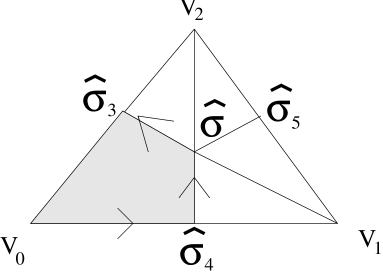
Figure 3: Barycentres of $K$.

We can now construct the dual description of a triangulation K. Geometrically this utilises a discrete analogue of the Hodge ${\mathbb{*}}$ operator. Recall the * operator maps a p-form to a $(D-p)$-form , where D is the dimension of the manifold M on which the p-form is defined. In the dual geometrical decomposition of the manifold, we want to set up a correspondence between a p-dimensional object and a $(D-p)$ dimensional object.

This is done as follows. We first construct $(D-p)$ dimensional objects whose vertices are barycentres of a sequence of successively higher dimensional simplices, where each simplex is a face of the following one. In other words $(D-p)$ dimensional objects of the form $\{\hat{\sigma}_{p},\hat{\sigma}_{p+1},\dots,\hat{\sigma}_{D}\}$, where $\sigma_{n}$ is a face of $\sigma_{n+1}$. The orientation of these are set so as to be compatible with the manifold. Joining these objects together gives us the dual of $\sigma_{p}$.

Thus for instance the map * acts on $[v_{0}]$ as follows.

$$*_{K}:[v_{0}]\to\epsilon_{01}[\hat{v_{0}},\hat{\sigma_{1}},\hat{\sigma}]\cup[\hat{v_{0}},\hat{\sigma_{3}},\hat{\sigma}]\epsilon_{03}.$$

Where the orientation of each of the small triangles has to be coherent with the orientation of the original triangle. This is shown in fig. 3 and leads to mapping $[v_{0}]$ to the shaded two dimensional region. The orientations of the simplices are specified by arrows in the figure. Coherence of orientation means, for example, that the arrow of an edge agrees with the arrow of the triangle to which it belongs. Next we consider $[v_{0},v_{1}]$. This is a 1-simplex and is to be mapped to a (2-1)=1 dimensional object. The map is defined as

$$*_{K}:[v_{0},v_{1}]\to[\hat{\sigma_{1}},\hat{\sigma}].$$

Again the orientation of $[\hat{\sigma_{1}},\hat{\sigma}]$ has to be coherent with the orientation of the triangles already introduced when the map for $[v_{0}]$ was considered. Similarly

$$*_{K}:[v_{1},v_{2}] \to [\hat{\sigma_{2}},\hat{\sigma}],$$

$${}_{K}:[v_{2},v_{0}] \to [\hat{\sigma_{3}},\hat{\sigma}],$$

and finally

$$*_{K}:[v_{0},v_{1},v_{2}] \to[\hat{\sigma}].$$

We then have the alternate discretisation $\hat{K}$ for M shown in fig. 4.

Figure 4: Dual complex $\hat{K}$.

Note when two edges are glued together they must have opposite orientations. We can now give the general rule for mapping an n-simplex $\sigma_{n}=[v_{0},\dots,v_{n}]$ to a ($D-n)$ dimensional object ( (D-n) cell) as follows: We think of $\sigma_{n}$ as an element of a simplicial complex K. We have

$$*_{K}:[v_{0},\dots,v_{n}]\to\cup[\hat{\sigma_{n}},\hat{\sigma_{n+1}},\dots,\hat{\sigma_{D}}],$$

where $\hat{\sigma}_{n+1}$ is the barycentre of an (n+1)-simplex which has $\sigma_{n}$ as a face. $\hat{\sigma}_{n+2}$ is the barycentre of an (n+2)-simplex which has $\sigma_{n+1}$ as a face and so on. These objects have to be coherently oriented with respect to $[v_{0},\dots,v_{n}]$. The set of these cells constitutes the dual space $\hat{K}$ of K.

By this procedure we claim, a discrete version of the Hodge star operation * has been constructed. Let us explain. The Hodge * operator involves forms. It maps p-forms in D dimensions to a (D-p)-form. The $*_{K}$ map involves not forms but geometrical objects. There is a simple correspondence relation between these two cases. Given a p-form, $\phi_{p}$, and a p-dimensional geometrical space, $\Sigma_{p}$, the p-form can be integrated over $\Sigma_{p}$ to give a number. Thus $\Sigma_{p}$ and $\phi_{p}$ are objects that can be paired. We can write this as a pairing

$$(\phi_{p},\Sigma_{p})=\int_{\Sigma_{p}}\phi_{p}.$$

In order to proceed, we need to introduce some more structure. We start by associating with a simplicial complex K, containing $\{\sigma_{p}^{i}\}$ $(i=1,\dots,K_{p};p=0,\dots,D)$ a vector space consisting of finite linear combinations over the reals of the p-simplices it contains. This vector space is known as the space of p-chains,$C_{p}(K)$. For two elements $\sigma_{p}^{i},\sigma_{p}^{j}\in C_{p}(K)$, a scalar product $(\sigma_{p}^{i},\sigma_{p}^{j})=\delta_{j}^{i}$ can be introduced. An oriented p-simplex changes sign under a change of orientation i.e. if $\sigma_{p}=[v_{0},\dots,v_{p}]$ and $\tau$ is a permutation of the indices $[0,\dots,p]$, then $[v_{\tau(0)},\dots,v_{\tau(p)}]=(-1)^{\tau}[v_{0},\dots,v_{p}]$, with $\tau$ denoting the number of transpositions needed to bring $[v_{\tau(0)},\dots,v_{\tau(p)}]$ to the order $[v_{0},\dots,v_{p}]$.

Given the vector space $C_{p}(K)$, the boundary operator $\partial^{K}$ can be defined as

$$\partial^{K}:C_{p}(K)\to C_{p-1}(K).$$

It is the linear operator which maps an oriented p simplex $\sigma^{(p)}$ to the sum of its (p-1) faces with orientation induced by the orientation of $\sigma^{p}$. If $\sigma^{p}=[v_{0},\dots,v_{p}]$, then

$$\partial\sigma^{p}=\sum_{i=0}^{p}(-1)^{i}[v_{o},\dots,\hat{v_{i}},\dots v_{p}],$$

where $[v_{o},\dots,\hat{v_{i}},\dots,v_{p}]$ means that the vertex $v_{i}$ has been omitted from $\sigma^{p}$ to produce the face “opposite” to it.

Given that $C_{p}(K)$ is a vector space, it is possible to define a dual vector space $C^{p}(K)$, consisting of dual objects known as cochains; that is we can take an element of $C_{p}(K)$ and an element $C^{p}(K)$ to form a real number. Since the space $C_{p}(K)$ has a scalar product, namely if $\sigma_{p}^{i},\sigma_{p}^{j}\in C_{p}(K)$ then $(\sigma_{p}^{i},\sigma_{p}^{j})=\delta_{ij}$. We can use the scalar product to identify $C_{p}(K)\equiv C^{p}(K)$, so that we can consider oriented p-simplices as elements of $C^{p}(K)$ as well as $C_{p}(K)$. We can write our boundary operation as

$$([v_{0},\dots,\hat{v_{i}},\dots,v_{p}],\partial^{K}[v_{0},\dots,v_{p}])=(-1)^{i}.$$

This suggests introducing the adjoint operation $d_{K}$ defined as

$$(d^{K}[v_{0},\dots,\hat{v_{i}},\dots,v_{p}],[v_{0},\dots,v_{p}])=([v_{0},\dots,\hat{v_{i}},\dots,v_{p}],\partial^{K}[v_{0},\dots,v_{p}]).$$

This is the coboundary operator which maps $C_{p}(K)\to C_{p+1}(K)$.

Indeed we have

$$d^{K}[v_{0},\dots,v_{p}]=\sum_{v}[v,v_{0},\dots,v_{p}],$$

where the sum is over all vertices $v$ such that $[v,v_{0},\dots,v_{p}]$ is a (p+1) simplex.

The boundary operators $\partial_{K}$ and the coboundary operator $d_{K}$ have the property $\partial_{K}\partial_{K}=d_{K}d_{K}=0$. Furthermore,

$$d_{K}:C_{p} \to C_{p+1},$$

$$\partial_{K}:C_{p} \to C_{p-1}.$$

These operators are the discrete analogues of the operators $d$ and $(-1)^{D(p+1)+1}*d*=d^{*}$ which act on forms.

These operators could be defined only when a scalar product(“metric”) was introduced in the vector space $C_{p}$’s. At this stage we have a discrete geometrical analogue of $d$, $d^{*}$ and $*$. We have also commented on the fact that the operation $*$ maps simplices into dual cells i.e. not simplices. If the original simplicial system is described in terms of the union of the vector spaces of all p-chains then the space into which elements of the vector space are mapped by * is not contained within this space, unlike the situation for the Hodge star operation on forms. We will see that this difference leads inevitably to a doubling of the fields when discretisation, preserving topological structures, is attempted.

We now need a way to relate a p-chain to a p-form. This together with a construction which linearly maps p-forms to p-simplices will allow us to translate expressions in continuum QFT to a corresponding discrete geometrical objects. We start with the construction of the linear maps from p-chains to p-forms due to Whitney [4].

In order to define this map, we need to introduce barycentric coordinates associated with a given p-simplex $\sigma^{p}$. Regarding $\sigma^{p}$ as an element of some ${\mathbb{R}}^{N}$, we introduce a set of real numbers $(\mu_{0},\dots,\mu_{p})$ with the property

$$\mu_{i} \geq 0,$$

$$\sum_{i}\mu_{i} = 1.$$

A point $x\in\sigma^{p}$ can be written in terms of the vertices of $\sigma^{p}$ and these real numbers as

$$x=\sum_{i=0}^{p}\mu_{i}v_{i}.$$

Note if any set of $\mu_{i}=0$ then the vector $x$ lies on a face of $\sigma^{p}$. One can think of $x$ as the position of the center of mass of a collection of masses $(\mu_{0},\dots,\mu_{p})$ located on the vertices $(v_{0}.\dots,v_{p})$ respectively. Setting $\mu_{i}=0$ for instance means the center of mass will be in the face opposite the vertex $v_{i}$. The Whitney map can now be defined. We have

$$W^{K}:C^{p}(K)\to\Phi^{p}(K),$$

where $\Phi^{p}(K)$ is a p-form. If $\sigma^{p}\in C^{p}(K)$ then

$$W[\sigma^{p}]=p!\sum^{p}_{i=0}(-1)^{i}\mu_{i}d\mu_{0}\wedge\dots\hat{d\mu_{i}}\wedge\dots d\mu_{p},$$

where $\hat{d\mu_{i}}$ means this term is missing, and $(\mu_{0},\dots,\mu_{p})$ are the barycentric coordinate functions of $\sigma^{p}$.

We next construct the linear map from p-forms to p-chains. This is known as the de Rham map. We have

$$A^{K}:\Phi^{p}(K)\to C^{p}(K),$$

defined by

$$<A^{K}(\Phi^{p}),\sigma^{p}>=\int_{\sigma^{p}}\Phi^{p},$$

for each oriented p-simplex $\in K$.

A discrete version of the wedge product can also be defined using the Whitney and de Rham maps such that $\wedge^{K}:C^{p}(K)\times C^{q}(K)\to C^{p+q}(K)$ as follows:

$$x\wedge^{K}y=A^{K}(W^{K}(x)\wedge W^{K}(y)).$$

It has many of the properties of the continuous wedge product in that it is skewsymmetric and obeys the Leibniz rule but it is nonassociative.

At this stage we have introduced all the building blocks necessary to discretise a system preserving geometrical structures. We summarize the properties of the maps introduced in the form of a theorem [4]:

1. $A^{K}W^{K}$ = Identity.
   

2. $dW^{K}=W^{K}d^{K}$, where $d:\phi^{p}\to\phi^{p+1}$.
   

3. $\int_{\mid\beta\mid}W^{K}(\alpha)=<\alpha,\beta>$, $\alpha,\beta\in K$
   

4. $d^{K}A^{K}=A^{K}d$.
   

This theorem shows how $d^{K}$ can be considered as the discrete analogue of $d$. We now show how $*^{K}$ can be considered as discrete analogue of $*$. For this we need barycentric subdivision.

We recall that given a simplicial complex $\{\sigma^{p}_{i}\}$, i=1,$\dots,K_{p};p=0,\dots,D$. A set of points(vertices) could be assigned to each simplex, namely $\hat{\sigma_{i}^{p}}$. These are the barycentres. These vertices, regarded as vertices of a simplex, subdivide the original simplices to give a finer triangulation of the original manifold. This is a barycentric subdivision map $BK$. Clearly the procedure can be repeated to give finer and finer subdivisions in which the simplices become “smaller”. The procedure is illustrated for a triangle in Fig. 5.

Figure 5: Barycentric subdivision of $K$.

Note that all the barycentres are present as vertices of the barycentric subdivision and that $*^{K}$ acting on simplices belonging to the simplicial complex, $K$, associated with $[v_{0},v_{1},v_{2}]$ leads to objects which are not, in general, simplices of $[v_{0},v_{1},v_{2}]$ but belong to a different space $\hat{K}$. However both $K$ and $\hat{K}$ are contained in the barycentric subdivision $B[v_{0},v_{1},v_{2}]$. This is a crucial observation. In order to construct the star map, two geometrically distinct spaces were introduced. The original simplicial decomposition $K$ with its associated set of p-chains $C^{p}(K)$ and the dual cell decomposition $\hat{K}$ with its associated set of p-chains $C^{p}(\hat{K})$. These spaces are distinct. However both belong to the first barycentric subdivision of $K$. This allows the use the $*^{K}$ operation if we think of $K$ and $\hat{K}$ as elements of $BK$.

We proceed as follows. Let BK and $\hat{K}$ denote the barycentric subdivision and dual triangulation, and

$$*^{K}:C^{p}(K)\to C^{n-p}(\hat{K}).$$

However $C^{p}(K)$ and $C^{p}(\hat{K})$ are both contained in $C^{p}(BK)$ as we have seen. Let

$$W^{BK}:C^{p}(BK)\to\phi^{p}(M),$$

denote the Whitney map. Then we have for $x\in C^{p}(K),y\in C^{n-p-1}(\hat{K})$[11]:

1. $<*^{K}x,y>=\frac{(n+1)!}{p!(n-p)!}\int_{M}W^{BK}(Bx)\wedge W^{BK}(By).\\ \\ <*^{\hat{K}}y,x>=\frac{(n+1)!}{p!(n-p)!}\int_{M}W^{BK}(By)\wedge W^{BK}(Bx).$
   
   

2. $\partial^{K}=(-1)^{np+1}*^{\hat{K}}d^{\hat{K}}*^{K}$ on $C^{p}(K)$.
   $\partial^{\hat{K}}=(-1)^{nq+1}*^{K}d^{K}*^{\hat{K}}$ on $C^{q}(\hat{K})$.
   

These are the discrete analogues of the interrelationships between $d,d^{*},*$ and $<\cdot,\cdot>$ in the continuum.

Note $K\neq\hat{K}$ and that properties of $\partial_{K},d_{K}$ analogous to those for differential forms only hold if $K$ , $\hat{K}$ are both regarded as elements of BK. This feature of the discretisation method is, as we shall see, crucial if we want to preserve topological properties of the original system. If a discretisation method is introduced without the $*$ operation in it then as we shall see in section 5 the topological properties of the partition function for the Abelian Chern-Simons gauge theory do not hold.

We proceed to apply these ideas to the Abelian Chern-Simons gauge theory on a compact three manifold $M$. First we summarize properties of the continuum field theory.

3 Schwarz’s topological field theory and the Ray-Singer torsion

We begin our treatment of continuum field theory by describing Schwarz’s method for evaluating the partition function of the Chern-Simons gauge theory on a three-manifold $M$ [16]. We assume that the first real homology group ( to be defined shortly) of the manifold vanishes; this is done for the sake of simplicity. Schwarz’s method is applicable for arbitrary compact 3-manifolds without boundary. Such manifolds are called “homology 3-spheres”. The main example we have in mind are the 3-sphere $S^{3}$ and the lens spaces $L(p,1)$, p=1, 2, $\dots$( for a definition and the basic properties of lens spaces see [17, 18]). The fields of the theory are the 1-forms on M i.e. $\omega\in\Omega^{1}(M)$. (In terms of a local coordinate system $(X^{\mu})$ on M we have $\omega(x)=\omega_{\mu}(x)dx^{\mu}$.) The action is

$$S(\omega)=\int_{M}\omega\wedge d_{1}\omega=\int_{M}dx^{1}dx^{2}dx^{3}\epsilon^{\mu\nu\rho}\omega_{\mu}\partial_{\nu}\omega_{\rho}.$$ (4)

Here and in the following $\Omega^{q}(M)$ denotes the space of $q$-forms on M (i.e. the antisymmetric tensor fields of degree q) and $d_{q}:\Omega^{q}(M)\to\Omega^{q+1}(M)$ i.e. the exterior derivative. It has the property $d_{q}d_{q-1}=0$ so ${\rm Im}(d_{q-1})\subset{\rm Ker}(d_{q})$, where $Im(d_{q-1})$ is the image of the operator $d_{q-1}$ while $Ker(d_{q})$ is the null space of the operator $d_{q}$ and the cohomology spaces $H^{q}(M)$ are defined by

$$H^{q}(M)={\rm Ker}(d_{q})/{\rm Im}(d_{q-1}).$$

The $H^{q}(M)$ are Abelian groups which contain topological information about the manifold. The vanishing of $H^{1}(M)$, for instance, holds if the manifold is simply connected that is any loop in $M$ can be smoothly deformed to any other loop in $M$ [14]. Note that $\Omega^{0}(M)$ is the space of functions on M and since $d_{0}$ is the derivative ${\rm Ker}(d_{0})$ consists of the constant functions i.e.

$$H^{0}(M)={\rm Ker}(d_{0})/{0}={\rm Ker}(d_{0})={\mathbb{R}}.$$

Our requirement on M that $H^{1}(M)=0$ implies that

$${\rm Im}(d_{0})={\rm Ker}(d_{1}).$$

A choice of metric on M determines an inner product in the spaces $\Omega^{q}(M)$ and allows the action (4) to be written as

$$S(\omega)=\lambda<\omega,(*d_{1})\omega>,$$ (5)

where * is the Hodge star operator. ( See [13] for background on this and other differential-geometric constructions.) In order to evaluate the partition function of this action by Schwarz’s method requires the introduction of the resolvent for $S(\omega)$. The partition function is defined as

$$Z(\lambda) = N\int d\omega e^{iS(\omega)}.$$

The main problem in evaluating $Z(\lambda)$ is to properly deal with the zeroes of $S(\omega)$. These zero modes contain topological information regarding the manifold as the space of zero modes is given by ${\rm Ker}(d_{1})$ and hence should not be discarded. Schwarz introduced an algebraic method (the resolvent method) for dealing with this problem. Although it is only valid for $S(\omega)$’s which are quadratic in $\omega$, it can be used to analyse $S(\omega)$’s constructed on arbitrary compact manifolds without boundary. For systems of this type Schwarz’s method is an algebraic analogue of the problem of gauge fixing. The advantage of the resolvent method is that it can be easily extended to deal with the process of discretisation as we will show.

The resolvent is defined to be the following chain of maps

$$0\to{\mathbb{R}}\to^{\phi_{0}}\Omega^{0}(M)\to^{d_{0}}{\rm Im}(d_{0})={\rm Ker}(d_{1})\to{\rm Ker}(S)\to 0.$$ (6)

These chain of maps form an exact sequence, that is, the image of a map is the kernal of the map which follows. With the help of the resolvent, Schwarz was able to show that the partition function for the theory was given by [16]

$$Z(\lambda)=e^{-\frac{i\pi}{4}\iota}(\frac{\lambda}{\pi})^{-\frac{\zeta}{2}}{\det}^{\prime}((*d_{1})^{2})^{-\frac{1}{4}}{\det}^{\prime}(d^{*}_{0}d_{0})^{\frac{1}{2}}\det(\phi_{0}^{*}\phi_{0})^{-\frac{1}{2}},$$ (7)

where $\iota$ is a non-topological geometry dependent function and $\zeta$ as shown in [11] is given by

$$\zeta={\rm dim}H^{0}(M)-{\rm dim}H^{1}(M).$$

$\iota$ is part of a phase factor and thus the absolute value of the partition function $Z(\lambda)$ is a topological quantity. This will be our main concern [10].

For completeness we give a quick proof of this result, ignoring phase factors and constants.

Introducing a metric in the space of $\omega$’s allows us to write

$$Z(\lambda) = N\int_{{\rm Ker}d_{1}\oplus({\rm Ker}d_{1})^{\perp}}d\omega e^{iS(\omega)},$$

$$= \mbox{Vol}({\rm Ker}d_{1})\cdot(\det d_{1}^{*}d_{1})^{-\frac{1}{4}}N.$$

We proceed to rewrite Vol(${\rm Ker}d_{1}$) using the exact sequence associated with ${\rm Ker}d_{1}$ and the manifold $M$. This procedure gives an expression for the partition function $Z$ containing information about the spaces ${\rm Ker}d_{1}$ and $({\rm Ker}d_{1})^{\perp}$. Simply dropping Vol(Ker$d_{1}$) leads to a loss of information. We have Vol(${\rm Ker}S$)=Vol(${\rm Ker}d_{1}$) = Vol(${\rm Im}d_{0}$) by assumption (if $H_{1}(M)$ is non-trivial, this equation has to be modified [8]). Also,

$$d_{0}\mid_{({\rm Ker}d_{0})^{\perp}}:({\rm Ker}d_{0})^{\perp} \to ({\rm Im}d_{0})$$

$$\Rightarrow\mbox{Vol}({\rm Im}d_{0}) = \mid{\det}^{\prime}d_{0}\mid\mbox{Vol}({\rm Ker}d_{0})^{\perp}.$$

Note

$$\Omega^{0} = {\rm Ker}d_{0}\oplus({\rm Ker}d_{0})^{\perp}$$

and

$$\phi_{0}:{\cal H}_{0} \to H_{0}$$

$$\mbox{Vol}(H_{0}) = \mid\det\phi_{0}\mid\mbox{Vol}({\cal H}_{0}).$$

where ${{\cal H}}_{\rm 0}$ represents the space of harmonic $0$-forms. Note harmonic $p$-forms are solutions of $(d^{*}d+dd^{*})\phi_{p}=0$. In this space the Hodge star operator is present and hence a scalar product and volume can be defined. The map $\phi_{0}$ introduced relates the space of harmonic $0$-forms to the space of de Rham cohomology $H_{0}$. By a theorem of Hodge this space of harmonic $p$-forms is isomorphic to the space of $H_{p}$[13]. The space of de Rham cohomology does not have a metric and hence we define the volume in this space with the help of the map $\phi_{0}$. Therefore,

$$\mbox{Vol}({\rm Ker}d_{0})^{\perp} = \mbox{Vol}(\Omega_{0})[\mbox{Vol}({\rm Ker}d_{0})]^{-1},$$

$$= \mbox{Vol}(\Omega_{0})(\mbox{Vol}(H_{0}))^{-1},$$

$$= (\mbox{Vol}(\Omega_{0}))(\det\phi_{0})^{-1}(\mbox{Vol}({\cal H}_{0}))^{-1}.$$

So that finally we get

$$\mbox{Vol}({\rm Ker}S)=\mid{\det}^{\prime}d_{o}\mid\mid\det\phi_{0}\mid^{-1}\mbox{Vol}(\Omega_{0})(\mbox{Vol}{\cal H_{0}})^{-1}.$$

Choosing

$$N\mbox{Vol}(\Omega_{0})(\mbox{Vol}{\cal H_{0}})^{-1}=1,$$

we get

$$Z=\mbox{Vol}({\rm Ker}S)(\det d_{1}^{*}d_{1})^{-\frac{1}{4}}=\mid{\det}^{\prime}d_{0}\mid\mid\det d_{1}d^{*}\mid^{-\frac{1}{4}}\mid\det\phi_{0}\mid^{-1}.$$

A more careful calculation gives the determinant in (7). The quantities $\iota$ and $\zeta$ in (7) also need to be zeta-regularised - this was done in [11], where it was shown that the regularised $\zeta$ is given by

$$\zeta={\rm dim}H^{0}(M)-{\rm dim}H^{1}(M).$$

So in the present case, where $H^{0}(M)\equiv{\mathbb{R}}$ and $H^{1}(M)=0$, we have

$$\zeta=1-0=1.$$ (8)

Using the formulae $d_{1}^{*}=*d_{1}*$ and $**=1$ (modulo a possible sign), we get $d_{1}=*d_{1}^{*}*$ and therefore $(*d_{1})^{2}=*d_{1}*d_{1}=d_{1}^{*}d_{1}$, which gives

$${\det}^{\prime}((*d_{1})^{2})={\det}^{\prime}(d_{1}^{*}d_{1}).$$ (9)

Substituting (8) and (9) in (6) we get

$$Z(\lambda)=e^{-\frac{i\pi}{4}\iota}(\frac{\lambda}{\pi})^{-\frac{\zeta}{2}}{\det}^{\prime}(d_{1}^{*}d_{1})^{-\frac{1}{4}}{\det}^{\prime}(d^{*}_{0}d_{0})^{\frac{1}{2}}\det(\phi_{0}^{*}\phi_{0})^{-\frac{1}{2}}.$$ (10)

We now rewrite the product of determinants in (10) in terms of the Ray-Singer torsion [20] of M. Since the Hodge star operator * is unitary with $**=1$ and $d_{0}^{*}=*d_{2}*$ (modulo a possible sign) we have

$${\det}^{\prime}(d^{*}_{0}d_{0}) = {\det}^{\prime}(*d_{2}*d_{0})={\det}^{\prime}(*(*d_{2}*d_{0})*),$$

$$= {\det}^{\prime}(d_{2}*d_{0}*)={\det}^{\prime}(d_{2}d_{2}^{*}),$$

$$= {\det}^{\prime}(d_{2}^{*}d_{2}).$$

It follows that

$${\det}^{\prime}(d_{0}^{*}d_{0})^{\frac{1}{2}}{\det}^{\prime}(d_{1}^{*}d_{1})^{-\frac{1}{4}}=({\det}^{\prime}(d_{0}^{*}d_{0})^{\frac{1}{2}}\det(d_{1}^{*}d_{1})^{-\frac{1}{2}}{\det}^{\prime}(d_{2}^{*}d_{2})^{\frac{1}{2}})^{\frac{1}{2}}.$$ (11)

It is possible to rewrite $\det(\phi^{*}_{0}\phi_{0})$ using a standard result of manifold theory in a different form(see [21]). We start by noting that the integration map

$$\int_{M}:H^{3}(M)\to{\mathbb{R}}$$

is an isomorphism, i.e. for each $r\in{\mathbb{R}}$ there is a unique class $[\alpha]\in H^{3}(M)$ such that $\int\alpha=r$. (Note that the integration map is well defined on $H^{3}(M)$ since $\int_{M}\alpha+d\beta=\int_{M}\alpha$ i.e. $\int_{M}d\beta=0$ by Stokes theorem.) Also from the definition

$$H^{3}(M)=\Omega^{3}(M)/{\rm Im}(d_{2})=({\rm Im}(d_{2})\oplus{\rm Im}(d_{2})^{\perp})/{\rm Im}(d_{2})={\rm Im}(d_{2})^{\perp},$$

it follows that the map given by

$${\rm Im}(d_{2})^{\perp}\to{\mathbb{R}}$$ (12)

is also an isomorphism. Now define the map

$$\phi_{3}:{\mathbb{R}}\to{\rm Im}(d_{2})^{\perp}$$

to be the inverse of (12). Then using the properties of the Hodge star operator it can be shown that

$$\det(\phi_{3}^{*}\phi_{3})=\det(\phi_{0}^{*}\phi_{0})^{-1}.$$

It follows that

$$\det(\phi_{0}^{*}\phi_{0})^{-\frac{1}{2}}=(\det(\phi_{0}^{*}\phi_{0})^{-\frac{1}{2}}\det(\phi_{3}^{*}\phi_{3})^{\frac{1}{2}})^{\frac{1}{2}}.$$ (13)

Substituting (13) and (11) in (10) we get

$$\mid Z(\lambda)\mid=(\frac{\lambda}{\pi})^{-\frac{1}{2}}\tau_{RS}(M)^{\frac{1}{2}},$$ (14)

where

$$\tau_{RS}(M)=\det(\phi_{0}^{*}\phi_{0})^{-\frac{1}{2}}\det(\phi_{3}^{*}\phi_{3})^{\frac{1}{2}}{\det}^{\prime}(d^{*}_{0}d_{0})^{\frac{1}{2}}{\det}^{\prime}(d_{1}^{*}d_{1})^{-\frac{1}{2}}{\det}^{\prime}(d^{*}_{2}d_{2}).$$ (15)

This quantity $\tau_{RS}(M)$ is the Ray-Singer torsion of M [20]. It is a topological invariant of M i.e. is independent of the metric of M. Thus the modulus $\mid Z(\lambda)\mid$ of the partition function, given by (13)-(14), is a topological invariant.

We are now ready to construct a discrete version of the preceding topological field theory which reproduces the continuum expression for the partition function where subdivision invariance is the discrete property corresponding to topological invariance. We will see that in order to do this it is crucial that there is an analogue of the Hodge star operator in the discrete theory. As we will see in the next section, this requires a field doubling. Therefore we consider a doubled version of the preceding theory, with the fields $\omega_{1}$ and $\omega_{2}$ in $\Omega^{1}(M)$ and with the action functional (5) changed by

$$S(\omega)=\lambda<w,(*d_{1})w>\to\tilde{S}(\omega_{1},\omega_{2})=\lambda<({}^{\omega_{1}}_{\omega_{2}}),({}^{\,\,0\,\,\,*d_{1}}_{*d_{1}\,\,0})({}^{\omega_{1}}_{\omega_{2}})>.$$ (16)

The reason for this specific choice of action $\tilde{S}(\omega_{1},\omega_{2})$ for the doubled theory will become clear in the next section. An obvious generalisation of the proceeding, with $T\to\tilde{T}=({}^{\,\,0\,\,\,*d_{1}}_{*d_{1}\,\,0})$ shows that the partition function of the doubled theory

$$\tilde{Z}(\lambda)=\int_{\Omega^{1}(M)\times\Omega^{1}(M)}{\cal D}\omega_{1}{\cal D}\omega_{2}e^{-\lambda\tilde{S}(\omega_{1},\omega_{2})}$$

can be evaluated to obtain the square of (15)

$$\tilde{Z}(\lambda)=\mid Z(\lambda)\mid^{2}=(\frac{\lambda}{\pi})^{-1}\tau_{RS}(M).$$ (17)

Note that there is no phase factor here. This is because the quantity $\iota=d_{+}+d_{-}$ for the action $\tilde{S}$ in (16) vanishes since $\tilde{T}=({}^{\,\,0\,\,\,*d_{1}}_{*d_{1}\,\,0})$ has a symmetric spectrum.

4 The discrete version of the topological field theory

We proceed to construct a discrete version of Abelian Chern-Simons gauge theory. The Whitney map enables the Abelian Chern-Simons theory to be discretised by replacing the gauge field (1-form) $A\in\Omega^{1}(M)$ by the discrete analogue, a 1-cochain $x\in C^{1}(K)$.

The most immediate way to do this is to construct the action $S_{K}$ of the discrete theory by

$$\lambda S_{K}(x)=\lambda S(W^{K}(x))=\lambda\int_{M}dW^{K}(x)\wedge W^{K}(x).$$

This can be shown to coincide with the discrete action for the Abelian Chern-Simons theory introduced in [6]. This prescription fails however, in the sense that the resulting partition function $Z_{K}(\lambda)$ is not a topological invariant i.e. is not independent of $K$, and does not reproduce the continuum expression for the partition function. We demonstrate this by considering the resolvent for $S_{K}$ obtained in an analogous way to the resolvent of the continuum action $S$ described in the previous section. Let $T_{K}:C^{1}(K)\to C^{1}(K)$ denote the self-adjoint operator on $C^{1}(K)$ determined by

$$S_{K}(x)=\int_{M}dW^{K}(x)\wedge W^{K}(x)=<T_{K}x,x>.$$

Then

$${\rm Ker}(T_{K})\subset{\rm Ker}(d_{1}^{K}).$$

Since for $x\in{\rm Ker}(d_{1}^{K})$ we have

$$<T_{K}x,x> = \int_{M}dW^{K}(x)\wedge W^{K}(x),$$ (18)

$$= \int_{M}W^{K}(d_{1}^{K}x)\wedge W^{K}(x).$$ (19)

Thus the discrete analogue of the resolvent (6) is a resolvent for $S_{K}$:

$$0\to{\mathbb{R}}\to^{\phi_{0}}\to\Omega^{0}(M)\to^{d_{0}^{K}}{\rm Ker}(d_{1}^{K})\subseteq{\rm Ker}(T_{K})={\rm Ker}(S_{K})\to 0.$$

The resulting partition function is the discrete analogue of the partition function $Z(\lambda)$:

$$Z_{K}(\lambda)={\det}^{\prime}((\phi_{0}^{K})^{*}\phi_{0}^{K})^{-\frac{1}{2}}{\det}^{\prime}((d_{0}^{K})^{*}d_{0}^{K})^{\frac{1}{2}}{\det}^{\prime}(-\frac{i\lambda}{\pi}T_{K})^{-\frac{1}{2}}.$$

In [11] the following formula for $T_{K}$ was obtained:

$$T_{K}[v_{0},v_{1}]=\frac{1}{6}\sum[v_{2},v_{3}]$$

where the sum is over all $1$-simplices $[v_{2},v_{3}]$ such that $[v_{0},v_{1},v_{2},v_{3}]$ is a $3$-simplex with orientation compatible with the orientation of $M$.

It is possible to show [8] that $\det((\phi_{0}^{K})^{*}\phi_{0}^{K})=N_{0}^{K}={\rm dim}C^{(K)}=$ the number of vertices of $K$. Then the failure of the discretisation prescription can be demonstrated by showing that the quantity

$$\mid Z(\lambda)\mid^{2}=\frac{1}{N_{0}^{K}}{\det}^{\prime}(\partial_{1}^{K}d_{0}^{K}){\det}^{\prime}(T_{K}^{2})^{-\frac{1}{2}}$$

is not independent of $K$.

A discrete version of the doubled topological field theory with action (16) has been constructed in [11] in such a way that the expression (17) for the continuum partition function is reproduced. We briefly describe this in the following.

The discretisation prescription is

$$(\omega_{1},\omega_{2})\in\Omega^{1}(M)\times\Omega^{1}(M)\to(x,y)\in C^{1}(K)\times C^{1}(\hat{K}),$$ (20)

$$S(\omega)=\lambda<({}^{\omega_{1}}_{\omega_{2}}),({}^{\,\,0\,\,\,*d_{1}}_{*d_{1}\,\,0})({}^{\omega_{1}}_{\omega_{2}})>\to\tilde{S}_{K}(x,y)=\lambda<({}^{x}_{y}),({}^{\,\,\,\,0\,\,\,\,\,\,\,\,*^{K}d^{K}}_{*^{\hat{K}}d^{\hat{K}}\,\,\,\,0})({}^{x}_{y})>,$$ (21)

where $K$ is the simplicial complex triangulating M, $\hat{K}$ is its dual, $C^{q}(K)$, $C^{p}(\hat{K})$, $d^{K}$ and $d^{\hat{K}}$ are as described in the previous section. The analogue of the Hodge star operator is the duality operator $*^{K}$. This is a map $*^{K}:C^{q}(K)\to C^{z-q}(\hat{K})$ ( and $*^{\hat{K}}:C^{p}(\hat{K})\to C^{z-p}(K)$ which explains the need for field doubling and the expression (21) for the discrete action $\tilde{S}_{K}(x,y)$. There is a natural choice of resolvent for $\tilde{S}_{K}(x,y)$, analogous to the resolvent (6) in the continuum case. It is

The partition function is

$$\tilde{Z}_{K}(\lambda)=\int_{C^{1}(K)\times C^{1}(\hat{K})}{\cal D}x{\cal D}ye^{-\tilde{S}_{K}(x.y)}.$$ (22)

Evaluating this by Schwarz’s method with the resolvent above leads to:

$$\tilde{Z}_{K}(\lambda)= (\frac{\lambda}{\pi})^{-1+N_{0}^{K}-N_{1}^{K}}\det((\phi_{0}^{K})^{*}\phi_{0}^{K})^{-\frac{1}{2}}{\det}^{\prime}((d_{0}^{K})^{*}d_{0}^{K})^{\frac{1}{2}}{\det}^{\prime}((d_{1}^{K})^{*}d_{1}^{K})^{-\frac{1}{4}},$$

$$\det((\phi_{0}^{\hat{K}})^{*}\phi_{0}^{\hat{K}})^{-\frac{1}{2}}{\det}^{\prime}((d_{0}^{\hat{K}})^{*}d_{0}^{\hat{K}})^{\frac{1}{2}}{\det}^{\prime}((d_{1}^{\hat{K}})^{*}d_{1}^{\hat{K}})^{-\frac{1}{4}}.$$

There is no phase factor in (22) since $\zeta$ vanishes just like in (17). We have also used the fact that $\zeta=1-N_{0}^{K}+N_{1}^{K}$ which is shown in [11].

Now rewrite the determinant involving $\hat{K}$ - objects in terms of determinants of $K$-objects. Modulo a possible sign $\pm$ we have the formulae[11]

$$(*^{\hat{K}})^{-1} =(*^{\hat{K}})^{*}=*^{K},$$ (23)

$$(*^{K})^{-1} =(*^{K})^{*}=*^{\hat{K}},$$ (24)

$$(d_{q}^{K})^{*} =*^{\hat{K}}d^{\hat{K}}_{n-q-1}*^{K},$$ (25)

$$(d_{p}^{\hat{K}})^{*} =*^{K}d_{n-p-1}^{K}*^{\hat{K}}.$$ (26)

( The $\pm$ signs are omitted because they will all cancel out in the following calculation.) Now:

$${\det}^{\prime}((d_{0}^{\hat{K}})^{*}d_{0}^{\hat{K}}) ={\det}^{\prime}(*^{K}d_{2}^{K}*^{\hat{K}}d_{0}^{\hat{K}}),$$ (27)

$$={\det}^{\prime}(*^{\hat{K}}(*^{K}d_{2}^{K}*^{\hat{K}}d_{0}^{\hat{K}})*^{K})$$ (28)

$$={\det}^{\prime}(d_{2}^{K}*^{\hat{K}}*^{K}),$$ (29)

$$={\det}^{\prime}(d_{2}^{K}(d_{2}^{K})^{*})$$ (30)

$$={\det}((d_{2}^{K})^{*}d_{2}^{K}),$$ (31)

and

$${\det}^{\prime}((d_{1}^{\hat{K}})^{*}d_{1}^{\hat{K}}) ={\det}^{\prime}(*^{K}d_{1}^{K}*^{\hat{K}}d_{1}^{\hat{K}}),$$ (32)

$$={\det}^{\prime}(*^{\hat{K}}(*^{K}d_{1}^{K}*^{\hat{K}}d_{1}^{\hat{K}})*^{K})$$ (33)

$$={\det}^{\prime}(d_{1}^{K}*^{\hat{K}}*^{K}),$$ (34)

$$={\det}^{\prime}(d_{1}^{K}(d_{1}^{K})^{*})$$ (35)

$$={\det}((d_{1}^{K})^{*}d_{1}^{K}).$$ (36)

The integration map (12) has a discrete analogue

$${\rm Ker}(d_{2}^{K})^{\perp} \to {\mathbb{R}},$$

$$a \to <a,[M]>,$$ (37)

where $[M]\in C_{3}(K)$, the orientation cycle of $M$, i.e. the sum of all 3-simplices of $K$, oriented so that their orientations are compatible with the orientation of $M$. ( Note that $a\in{\rm Ker}(d_{2}^{K})^{\perp}\subset C^{3}(K)$ can be evaluated on any element $\sigma\in C_{3}(K)$ to get a real number $<a,\sigma>\in{\mathbb{R}}$.) Define the map

$$\phi_{3}^{K}:{\mathbb{R}}\to{\rm Ker}(d_{2}^{K})^{\perp}$$ (38)

to be the inverse of (37). Then using the properties of $*^{K}$ and $*^{\hat{K}}$, it can be shown that

$$\det((\phi_{3}^{K})^{*}\phi_{3}^{K})=\det((\phi_{0}^{\hat{K}})^{*}\phi_{0}^{\hat{K}})^{-1}.$$ (39)

Now using (39), (31) and (36) we can rewrite (22) as

$$\tilde{Z}_{K}(\lambda)=(\frac{\lambda}{\pi})^{-1+N_{0}^{K}-N_{1}^{K}}\tau_{K}(M),$$ (40)

where

$$\tau_{K}(M)=\det((\phi_{0}^{K})^{*}\phi_{0}^{K})^{-\frac{1}{2}}\det((\phi_{3}^{K})^{*}\phi_{3}^{K})^{\frac{1}{2}}\prod_{q=0}^{2}{\det}^{\prime}((d_{q}^{K})^{*}d_{q}^{K})^{-\frac{1}{2}(-1)^{q}}.$$ (41)

This quantity $\tau_{K}(M)$ is the R-torsion of the triangulation $K$ of $M$. It is a combinatorial invariant of $M$ i.e. is independent of the choice of triangulation $K$ [22, 23, 24].

This is the untwisted torsion of $M$, more generally the torsion can be “twisted” by a representation of $\pi_{1}(M)$. The factors involving the determinants $\det^{\prime}((d_{q}^{K})^{*}d_{q}^{K})$ constitute the usual Reidemeister torsion of $M$ [19]. When these are put together with the factors involving $\det((\phi_{i}^{K})\phi_{i}^{K})$, $i=0,3$, as in (41) we get the R-torsion “as a function of the cohomology” introduced and shown to be triangulation-independent in [20].

The expression (41) for $\tau_{K}(M)$ is analogous to the expression (15) for the R-torsion $\tau_{RS}(M)$, and in fact it has been shown [22, 23] that these torsions are equal

$$\tau_{K}(M)=\tau_{RS}(M).$$

It follows that the partition function (40) of the discrete theory coincides with the partition function (15) of the continuum theory, except for the $K$-dependent quantities $N_{0}^{K}$ and $N_{1}^{K}$ appearing in (40). These quantities can be removed by a suitable $K$-dependent renormalisation of the coupling parameter $\lambda$.

It is possible to show that [8]

$$\det((\phi_{0}^{K})^{*}\phi_{0}^{K}) =N_{0}^{K}$$

$$\det((\phi_{3}^{K})^{*}\phi_{3}^{K}) =\frac{1}{N_{3}^{K}}.$$

We will use this result in our numerical work.

5 Numerical Results

We are now in a position to proceed to numerically evaluate the discrete expressions for the torsion obtained. This allows us to check the underlying theoretical ideas by numerically verifying that the discrete expressions agree with expected analytic results. It also allows us to check that the results obtained are subdivision invariant. The subdivision invariance of torsion is demonstrated by showing that if any simplex of the triangulation is subdivided, the value of the torsion does not change. This is what is meant by topological invariance in the discrete setting. The expected analytic result for torsion for a lens space $L(p,1)$ is (See [20])

$$T(L(p,1))=\frac{1}{p}.$$

Thus $T(S^{3})=T(L(1,1))=1$.

We also show, numerically, that the discrete expression for the Chern-Simons partition function obtained without using the * operator is not a topological invariant. This shows very clearly the importance of the doubling construction method used in the discretisation method, for capturing topological information.

In order to proceed, we need to efficiently triangulate the spaces $S^{3}$ and L(p,q). First we triangulate $S^{3}$. We do this by considering a four dimensional simplex $[v_{0},v_{1},v_{2},v_{3},v_{4}]$ and observing that the boundary of this object is precisely the triangulation $K$ of $S^{3}$ which we require. Next we turn to spaces L(p,q) which we need to triangulate in order to proceed. An efficient triangulation of this space has been constructed by Brehm and Swiatkowski [25]. We use this procedure for our computations [26].

We can now summarise our numerical results. The R-torsion for a simplicial complex $K$, with dual cell complex $\hat{K}$, for either $S^{3}$ or L(p,1) involves evaluating

$$T=\sqrt{\frac{1}{N_{0}N_{3}}\det(\partial_{1}d_{0})\det(\partial_{2}d_{1})^{-1}\det(\partial_{3}d_{2})},$$

where $N_{i}=$nos. of $i$-simplices in $K$, $\partial_{1},\partial_{2},\partial_{3}$ are boundary operators on $K$ and $d_{0},d_{1},d_{2}$ are coboundary operators on $K$. Note that, in the discrete setting, these operators can be expressed as matrices. We do this by using the vertices, edges, faces and tetrahedra of our complex as a basis list. Any $p$-simplex in the complex can then be expressed in terms of this. Since we know what $d$ maps the various basis list elements to, we can set the coefficients of its matrix representation. When we say $\det(\partial_{1}d_{0})$, for example, we simply mean the determinant of the matrix which results from multiplying the matrices corresponding to the operators $\partial_{1}$ and $d_{0}$.

If our complex consisted of just one triangle $[0,1,2]$, the basis list would be:

$$\begin{array}[]{lc}0&[0],\\ 1&[1],\\ 2&[2],\\ 3&[0,1],\\ 4&[0,2],\\ 5&[1,2],\\ 6&[0,1,2].\end{array}$$

We know that $d[0]=[1,0]+[2,0]$. This can be expressed in terms of our basis list as $d$ acting on basis element $0$ going to $-3-4$. So the matrix $d$ for this complex is:

$$\left(\begin{array}[]{ccccccc}0&0&0&0&0&0&0\\ 0&0&0&0&0&0&0\\ 0&0&0&0&0&0&0\\ -1&1&0&0&0&0&0\\ -1&0&1&0&0&0&0\\ 0&-1&1&0&0&0&0\\ 0&0&0&1&-1&1&0\\ \end{array}\right).$$

Note that the last column is zero since $d$ has nothing to map a $2$-simplex to and that the first three rows are zero since nothing is mapped to $0$-simplices. If we act on $0$ with this matrix we get $-3-4$, as expected, and $d^{2}=0$.

If we do not use $\hat{K}$ then from section 4,

$$\hat{T}=\mid Z(1)\mid^{2}=\frac{1}{N_{0}^{K}}({\det}^{\prime}\partial_{1}^{K}d_{0}^{K})(\det T_{K}^{2})^{-\frac{1}{2}}.$$

We evaluated the quantity $\hat{T}$ numerically for various triangulations $K$ of $S^{3}$ and found the following results shown in Table 2 for the change of $\hat{T}$ under subdivision where $m-n$ corresponds to a triangulation of $S^{3}$ with $n$ vertices and $m$ tetrahedra and where $X_{i}=\det\partial_{i}d_{i-1}$.

Complex	$X_{1}$	NEW	$\frac{X_{1}*X1}{NEW}$	$N_{3}$	$N_{0}$	$Z^{4}$
5-5	125	15625	1	5	5	0.04
8-6	1152	2985984	0.444	8	6	0.0123
9-6	2304	15116540	0.351	9	6	0.00975

Table 2: Results for $T$.

It is clear that $\hat{T}$ for $S^{3}$ is not subdivision invariant. We next evaluate $T$ for $S^{3}$ and for L(p,1) and check that it is indeed subdivision invariant and agrees with the analytic calculations for L(p,1), with p=2,3,4 and 5. These results are shown in Tables 4-6.

As a check on the numerical method we also count the number of zero modes of the Laplacian operator on the different p-chain spaces. These numbers gives the dimension of the Homology groups and are shown in Table 3.

p	No. of zero-modes of $\Delta_{p}$	Dim $H^{p}$
0	1	1
1	0	0
2	0	0
3	1	1

Table 3: Zero modes for $S^{3}$.

5.1 $S^{3}$

As a further check, a systematic way of carrying out subdivision known as the Alexander moves [27] was used to study the subdivision invariance of the torsion. There are four such moves in 3 dimensions. They are best explained by example. We have

1. $[0,1,2,3,4]->[x,1,2,3,4]+[0,x,2,3,4]$.

2. $[0,1,2,3,4]->[x,1,2,3,4]+[0,x,2,3,4]+[0,1,x,3,4]$.

3. $[0,1,2,3,4]->[x,1,2,3,4]+[0,x,2,3,4]+[0,1,x,3,4]+[0,1,2,x,4]$.

4. $[0,1,2,3,4]->[x,1,2,3,4]+[0,x,2,3,4]+[0,1,x,3,4]+[0,1,2,x,4]+[0,1,2,3,x]$.

These are all natural operations in that the first (nth) move corresponds to adding a vertex splitting the 1-simplex (n-simplex) $[0,1]$ ($[0,1,\dots,n]$) and connecting it to all the vertices resulting in two (n+1) tetrahedra.

The torsion T, in terms of its component determinants, and the way they change under the Alexander moves is exhibited in the table below,

Complex	$X_{1}$	$X_{2}$	$X_{3}$	$\frac{X_{1}*X_{3}}{X_{2}}$	$N_{3}$	$N_{0}$	T
s3	625	15625	625	25	5	5	1
a1s3	5184	$2.985984*10^{6}$	$2.7648*10^{4}$	48	8	6	1
a2s3	7776	$1.511654*10^{7}$	$1.04976*10^{5}$	54	9	6	1
a3s3	5184	$2.985984*10^{6}$	$2.7648*10^{4}$	48	8	6	1
a4s3	625	15625	625	25	5	5	1

Table 4: R-torsion for $S^{3}$.

where $X_{i}=\det\partial_{i}d_{i-1}$ and $a2s3$ means the complex which resulted after the type 2 Alexander moves were performed on the $S^{3}$. It’s clear from this that

$$T=\frac{1}{N_{3}N_{0}}\det(\partial_{1}d_{0})(\det\partial_{2}d_{1})^{-1}\det(\partial_{3}d_{2})$$

is subdivision invariant and thus a topological invariant of the manifold.

As a final check we tried several other subdivisions. We took a given triangulation and barycentric subdivided one or more ($n$) of its faces to get $1s3,2s3,\dots$ ($ns3$). The results are in Tables 4 and 5.

Complex	$X_{1}$	$X_{2}$	$X_{3}$	$\frac{X_{1}*X_{3}}{X_{2}}$	$N_{3}$	$N_{0}$	T
s3	625	$1.562*10^{4}$	625	25	5	5	1
1s3	5184	$2.985984*10^{6}$	$2.7648*10^{4}$	48	8	6	1
2s3	$3.9448*10^{4}$	$5.2166*10^{8}$	$1.018325*10^{6}$	77	11	7	1
3s3	$2.79936*10^{5}$	$8.418024*10^{10}$	$3.36798*10^{7}$	112	14	8	1
4s3	$1.876833*10^{6}$	$1.266709*10^{13}$	$1.032626*10^{9}$	153	17	9	1
5s3	$1.270325*10^{7}$	$2.037398*10^{15}$	$3.207653*10^{10}$	200	20	10	1

Table 5: R-torsion for $S^{3}$.

5.2 Lens spaces

We conclude with the results for the lens spaces. The results are shown in Table 6 . As can be seen, these agree extremely well with the known analytic result T(L(p,1))=$1/p$.

Complex	$X_{1}$	$X_{2}$	$X_{3}$	$\frac{X_{1}*X_{3}}{X_{2}}$	$N_{3}$	$N_{0}$	T
L(2,1)	$1.062937*10^{10}$	$3.618662*10^{29}$	$3.74484*10^{21}$	110	40	11	1/2
L(3,1)	$9.108*10^{12}$	$1.143589*10^{43}$	$1.08817*10^{32}$	86.666	60	13	1/3
L(4,1)	$1.1027*10^{16}$	$4.0468*10^{58}$	$2.89*10^{44}$	78.7487	84	15	1/4
L(5,1)	$1.790617*10^{19}$	$1.761432*10^{76}$	$7.49187*10^{58}$	76.16	112	17	1/5

Table 6: R-torsion for lens spaces.

6 Conclusions

The method of discretisation introduced works extremely well. The main point of the method is to construct discrete analogues for the set $(\Omega^{p},d,\wedge,*)$. Previous work in the direction has neglected the Hodge star operator, * [5, 28]. We have thus demonstrated that the Hodge star operator plays a vital role in the construction of topological invariant objects from field theory. We were able to construct an expression for the partition function which is correct even as far as overall normalisation is concerned. Mathematically the equivalence between the Ray-Singer torsion and the combinatorial torsion of Reidemeister was proved independently in 1976 by Cheeger [22] and Müller [23]. It is nice to see the result emerge in a direct manner by a formal process of discretisation. On the way we also had to double the original system so that K, the triangulation , and $\hat{K}$, its dual, are both present. If this doubling and the reason for it are overlooked, then the topological information present in the discretisation is lost, as our numerical results demonstrated.

It is clear that the geometry motivated discretisation method introduced is very general and that it can be used to analyse a wide variety of physical systems. In the approach outlined we have captured topological features. In applications capturing geometrical features of a problem are also very important. We are currently investigating this aspect of our approach.

A limitation of the method is that there is no simple generalisation to deal with non-abelian theories. The discrete analogies of $d$, $d^{\dagger}$ were linear : there is no natural discrete analogue of $d_{A}:=d+A$, with $A$ a Lie algebra valued one form.

References

- [1] K. G. Wilson, Phys. Rev., D10 (1974), 2445 .
- [2] M. Creutz, “ Quarks, Gluons and Lattices”, Cambridge University Press, Cambridge, 1983.
- [3] P. Becher and H. Joos, Z. Phys. C, 15 (1982), 343 .
- [4] H. Whitney, “Geometric Integration Theory”, Princeton University Press, Princeton, NJ, 1957.
- [5] S. Albeverio and B. Zegarlinski, Commun. Math. Phys., 132 (1990), 34.
- [6] S. Albevario and J. Schafer, J. Math. Phys., 36 (1995), 2157.
- [7] R. Loll, Discrete approaches to quantum gravity in four dimensions, gr-qc/9805049.
- [8] D. H. Adams, T.C.D. Thesis 1996.
- [9] David Adams, Samik Sen, Siddhartha Sen, James Sexton, Nuclear Physics B (Proc. Suppl), 63A-C (1998), 492-494.
- [10] D. H. Adams, Phys. Rev. Lett., 78 (1997), 4155.
- [11] D. H. Adams, R-Torsion and Linking Numbers from Simplicial Abelian Gauge Theories, T.C.D. Preprint hep-th/9612009.
- [12] For example:A. Phillips and D. Stone, Lattice Gauge Fields, Principal Bundles and The Calculation of Topological Charge, CMP 103(1986), 599; D. Birmingham and M. Rakowski, Discrete Quantum Field Theories and The Intersection Form, Mods. Phys. Lett. A, 9 (1994), 2265; N. Kawamoto, H. Nielsen, N. Sato, Lattice Chern-Simons Gravity via Ponzano-Regge Model, hep-th/9902165.
- [13] T. Eguchi, P. B. Gilkey and A. J. Hanson, Physics Reports 66, No.6 , 213-393, North-Holland Publishing Company (1980).
- [14] C. Nash and S. Sen, “Topology and Geometry for Physicists”, Academic Press, London, 1983.
- [15] J. G. Hocking and G. S. Young, “Topology”, Dover Publications, NY, 1961.
- [16] A. S. Schwarz, Lett. Math. Phys 2 (1978) , 247.
- [17] J.R. Munkres, “Elements of Algebraic Topology”, Addison Wesley Publishing Company, 1984.
- [18] D. Rolfsen, “Knots and Links”, Publish Or Perish, 1976.
- [19] J. Milnor, Bull. A.M.S, 72, (966), 348.
- [20] D. B. Ray and I. M. Singer, Adv. Math, 7,145(1971), Proceedings of Symposium in Pure Mathematics, Vol 23, p167(153).
- [21] M. Spivak, “A Comprehensive Introduction to Differential Geometry”, Publish or Perish, 1979.
- [22] J. Cheeger, Ann. Math 109 (1979), 259.
- [23] W. Müller, Adv. Math. 28 (1978), 233.
- [24] J. Dodzuik, Ann. J. Maths. 98 (1976), 79.
- [25] U. Brehm and J. Swiatkowski, Triangulations of Lens Spaces with few Simplices, SPB-288-59, 26pp (1993).
- [26] Samik Sen, T.C.D. M.Sc. Thesis 1997.
- [27] J. W. Alexander, Ann. Math, 31 (1930), 292-320.
- [28] D. Birmingham and M. Rakowski, Phys. Lett. B, 299, (1993) 299.