Casimir energy of a dilute dielectric ball with uniform velocity of light at finite temperature.

Abstract

The Casimir energy, free energy and Casimir force are evaluated, at arbitrary finite temperature, for a dilute dielectric ball with uniform velocity of light inside the ball and in the surrounding medium. In particular, we investigate the classical limit at high temperature. The Casimir force found is repulsive, as in previous calculations.

1 Introduction

Calculations of the Casimir energy for spherically symmetric boundary conditions have been the issue of numerous papers, since the first calculation by Boyer [1] (see also [2, 3, 4, 5, 6]). Although a general theory describing the fluctuations of the electromagnetic field at finite temperature has been present for a long time [7, 8, 9, 10, 11], the extension of the results for the dielectric ball from zero temperature to finite temperatures received less attention. The case of a conducting spherical boundary (at zero and finite temperature) was studied by Balian and Duplantier [2], and will serve here to verify the validity of the results we obtain. Brevik and Clausen [12], used the Debye asymptotic expansion to calculate the Casimir force on the dilute dielectric ball, assuming uniform velocity of light inside and outside the ball (including, however, frequency dependence of the permeability and permittivity), to leading order in the so–called dilute approximation (the nature of this approximation is explained following Eq.(16)). It turns out that the usual Debye approximation is most useful for zero temperature calculations, but involves complications at finite temperatures. For example, it was shown [13] that use of these asymptotics may lead to problematic results, such as that the Casimir energy of a dielectric ball is independent of temperature.

In this Letter we calculate the thermodynamic features of the Casimir effect for the dilute dielectric ball at finite temperature (to leading order in the dilute approximation). We obtain explicit simple expressions for the Casimir energy, free energy and for the Casimir force at arbitrary temperature. In particular, we find that (within the approximation made) the Casimir force is repulsive for any radius at any temperature (see Eq.(43)). At high temperature its leading behavior is proportional to ${T\over 16a^{3}\pi}$, where $a$ is the radius of the ball. Higher order corrections to the dilute approximation decay like powers of ${1\over T}$, and consequently the leading behavior ${T\over 16a^{3}\pi}$ gives the Casimir force quite accurately at high temperature (see section 5).

The starting point of the present calculation is an explicit expression for the Casimir energy density (to leading order in the dilute approximation). This expression was derived in [14] using simple properties of the Green’s function of the Helmholtz equation. The Casimir energy at finite temperature, $E_{C}(T)$, is then obtained by summing that explicit expression for the energy over the Matsubara frequencies. Then, using the usual thermodynamic relation between the Casimir free energy $F_{C}(T)$ and the Casimir energy $E_{C}(T)$, we obtain an explicit expression for $F_{C}(T)$ valid for all temperatures. We verify that $E_{C}(T)$ and $F_{C}(T)$ coincide at $T=0$, as they should (and the Casimir entropy vanishes at $T=0$). Furthermore, at high temperatures, $F_{C}(T)$ tends to a term which is proportional to $-T\log(aT)$ (where $a$ is the radius of the ball). This behavior is consistent with the results of [2] and is also consistent with the recent general discussion of the high–temperature classical limit in [15].

2 Mode summation at finite temperatures - general considerations

The eigenfrequencies of the electromagnetic field, subjected to some boundary conditions, are solutions of a set of characteristic equations

$$\Delta_{{\bf c}}^{k}(\omega)=0\hskip 28.45274ptk=1,2,3...$$ (1)

labeled by an index $k$. (The eigenfrequency spectrum is the union of solutions to all the equations in (1).) The set of parameters ${\bf c}$ describes the constraints, such as the radius of the sphere or the distance between the conducting plates. The functions $\Delta_{{\bf c}}^{k}(\omega)$ are usually expressions involving solutions of the scalar Helmholtz equation subjected to appropriate boundary conditions. In the following we consider the case of spherical symmetry, where the functions $\Delta_{{\bf c}}^{k}(\omega)$ involve combinations of Bessel functions (see Eq. (13-16) in sec. 3).

Let us first consider the system in its ground state at zero temperature. The zero temperature Casimir energy is of course the difference between the formally divergent sum over all allowed modes of the constrained system and the divergent sum over the modes of the free electromagnetic field,

$$E_{C}=\sum_{n}{\omega_{n}({\bf c})\over 2}-\sum_{n}{\omega_{n}^{\it free}\over 2}.$$ (2)

This expression is still divergent and needs regularization. Thus, we introduce a UV–frequency cut-off $\omega_{N}$ and define

$$E_{C}(\omega_{N})=\sum_{\omega_{n}\leq\omega_{N}}{\omega_{n}({\bf c})\over 2}-\sum_{\omega_{n}\leq\omega_{N}}{\omega_{n}^{\it free}\over 2}.$$ (3)

When the boundaries are pushed to infinity, the system ceases to be constrained and becomes free. This is described by letting the parameters c in (3) tend to an appropriate value, say, infinity. It is convenient to represent the sum in the last expression as a contour integral

$$E_{C}(\omega_{N})=\sum_{k}\oint_{\Gamma_{N}}\frac{z}{2}\,F_{k}(z;\mathbb{c})dz$$ (4)

where $\Gamma_{N}$ is shown on Fig.1, and

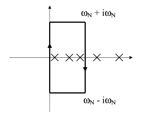
Figure 1: A rectangular contour in the complex plane.

$$F_{k}(z;\mathbb{c})=\lim_{\mathbb{c^{\prime}}\rightarrow{\it free}}\frac{1}{2\pi i}\frac{d}{dz}(\log\Delta_{\mathbb{c}}^{k}(z)-\log\Delta_{\mathbb{c^{\prime}}}^{k}(z)),$$ (5)

is the (regulated) resolvent corresponding to index $k$ in (1), and “${\it free}$” denotes the set of parameters describing the limiting case where the boundaries are taken to infinity. In the case of spherical geometry this is achieved by taking the radius to infinity. The Casimir energy is then defined as

$$E_{C}=\lim_{\omega_{N}\rightarrow\infty}E_{C}(\omega_{N}).$$ (6)

To carry over these considerations to finite temperature, we recall that the average energy per mode of the electromagnetic field is ${\omega\over 2}\coth(\beta\omega/2)$ and that the free energy per mode is $\frac{1}{\beta}\log(2\sinh(\beta\omega/2))$, where $\beta=\frac{1}{k_{B}T}$. Thus,

$$E_{C}(T;\omega_{N})=\sum_{k}\oint_{\Gamma_{N}}\frac{z}{2}\,\coth(\frac{\beta z}{2})F_{k}(z;\mathbb{c})dz,$$ (7)

is the (cut off) Casimir energy at temperature $T$, and

$$F_{C}(T;\omega_{N})=\sum_{k}\oint_{\Gamma_{N}}\frac{1}{\beta}\log(2\sinh(\beta z/2))F_{k}(z;\mathbb{c})dz,$$ (8)

is the (cut off) Casimir free energy at temperature $T$. Upon rotating the integration contour in (7) to wrap around the imaginary axis, the Casimir energy can be expressed as a sum over Matsubara modes, namely

$$E_{C}=\sum_{n=-\infty}^{\infty}\sum_{k}\left(\frac{z}{2}\,F_{k}(z;\mathbb{c})\right)\Big{|}_{z={2\pi in\over\beta}}.$$ (9)

This concludes our general considerations.

3 Casimir energy

In this section we study the temperature dependence of the Casimir energy of a dielectric ball, having permittivity and permeability $\epsilon,\mu$ which is embedded in a medium with permittivity and permeability $\epsilon^{\prime},\mu^{\prime}$. A further simplifying assumption which we make throughout this Letter, is that the velocity of light be continuous across the boundary, namely

$$\epsilon\mu=\epsilon^{\prime}\mu^{\prime}.$$ (10)

This condition is often desirable as it causes the frequency equations to simplify and some divergences to cancel out (see [16] and references therein). It turns out that in this case the energy depends on the dielectric data only through the parameter $\xi^{2}$ defined by

$$\xi^{2}=\left(\varepsilon_{1}-\varepsilon_{2}\over\varepsilon_{1}+\varepsilon_{2}\right)^{2}$$ (11)

which is symmetric under $\varepsilon_{1}\leftrightarrow\varepsilon_{2}$. Thus, the Casimir energy is invariant under interchanging the inner and outer media.

It has been shown [5, 14, 16] that under the condition (10), and after rotating the integration contour in (4) to the imaginary axis, that the difference in zero point energy of two balls of radii $a$ and $b$ may be written as

$$E_{C}(a)-E_{C}(b)=\sum_{l=1}^{\infty}(l+{1\over 2})\int^{\infty}_{\infty}d\omega\omega F_{l}(\omega;a,b),$$ (12)

where the resolvent (5) is

$$F_{l}(\omega;a,b)=-{1\over 2\pi}{d\over d\omega}\biggr{(}\log\big{[}1-\xi^{2}\lambda_{l}^{2}(a|\omega|)\big{]}-\log\big{[}1-\xi^{2}\lambda_{l}^{2}(b|\omega|)\big{]}\biggr{)}.$$ (13)

Here

$$\lambda_{l}(a|\omega|)=(s_{l}e_{l}(a|\omega|))^{\prime},$$ (14)

where $s_{l},e_{l}$ are the modified Bessel functions ($\nu=l+{1\over 2}$)

$$s_{l}(x)=ixj_{l}(ix)=\sqrt{\frac{\pi x}{2}}e^{-\frac{i\pi\nu}{2}}J_{\nu}(ix)$$ (15)

$$e_{l}(x)=ixh_{l}^{(1)}(ix)=i\sqrt{\frac{\pi x}{2}}e^{\frac{i\pi\nu}{2}}H^{1}_{\nu}(ix)$$ (16)

The case of $\xi$ finite but small corresponds to the inner ball being nearly identical in its properties to the surrounding medium. This is referred to in the literature as the limit of dilute media. In this limit we can expand (13) in powers of $\xi^{2}$. This expansion is further justified by the fact that on the imaginary $\omega$ axis $\lambda_{l}^{2}$ is small, thus the expansion can be pushed to $\xi^{2}\sim 1$ (for $\xi^{2}=1$, of course, one of the media has infinite conductivity and is thus a perfect conductor). In this Letter we will content ourselves with the leading term in this expansion. Thus, to order $\xi^{2}$ we have from (13)

$$F_{l}(\omega;a,b)={\xi^{2}\over 2\pi}{d\over d\omega}\biggr{(}\lambda_{l}^{2}(a|\omega|)-\lambda_{l}^{2}(b|\omega|)\biggr{)},$$ (17)

In [14] one of us was able to carry the sum over $l$ in (12) to first order in $\xi^{2}$ in closed form, without using Debye approximations, as is usually done in the literature. The result was

$$\xi^{2}\sum_{l=1}^{\infty}(l+\frac{1}{2})x\frac{d}{dx}\lambda_{l}^{2}(x)=\frac{\xi^{2}}{2}(-\frac{1}{2}+\frac{1}{2}e^{-4x}(1+2x)^{2}).$$ (18)

Thus, the relative resolvent, to order $\xi^{2}$, is

$$F^{(2)}(z;a,b)=\frac{\xi^{2}}{4\pi z}\left[e^{-4a|z|}(1+4a|z|+4a^{2}|z|^{2})-e^{-4b|z|}(1+4b|z|+4b^{2}|z|^{2})\right]$$ (19)

(here $z$ is a pure imaginary frequency.)

Using this simple explicit expression, we can calculate the energy in the dilute limit at an arbitrary temperature. In order to calculate the zero point energy with respect to the vacuum we take the limit $b\rightarrow\infty$ at the outset. Note that the $x$ independent term in (18) cancels between the two terms in the difference (19), resulting in an expression which decays exponentially when $|z|\rightarrow\infty$. Thus, no further regularization will be needed when we integrate over $\omega$. Using (9) and (19), the Casimir energy at temperature $T$ is

$$E_{C}(a,T)=\frac{\xi^{2}T}{4}\sum_{n=-\infty}^{\infty}e^{-8aT\pi|n|}(1+8aT\pi|n|+16a^{2}T^{2}\pi^{2}n^{2})=$$ (20)

$$\frac{\xi^{2}T}{4}\left(1-T\frac{\partial}{\partial T}+{T^{2}\over 4}\frac{\partial^{2}}{{\partial T}^{2}}\right){2\over e^{8a\pi T}-1}+\frac{\xi^{2}T}{4},$$

yielding

$$E_{C}(a,T)=\frac{T\xi^{2}}{4}+\frac{T\xi^{2}}{2\left(e^{8a\pi T}-1\right)}+\frac{4a\pi T^{2}\xi^{2}e^{8a\pi T}}{{{\left(e^{8a\pi T}-1\right)}^{2}}}+$$ (21)

$$\frac{8a^{2}\pi^{2}{T^{3}}\xi^{2}e^{8a\pi T}\left(1+e^{8a\pi T}\right)}{{\left(e^{8a\pi T}-1\right)}^{3}}$$

This result is exact (to order $\xi^{2}$) for all temperatures. It is immediate to check that as $T$ goes to zero we retain the correct zero temperature result [14]

$$E_{C}(a,0)=\frac{5\,\xi^{2}}{32a\pi}\,\,\,.$$ (22)

Note that at high temperatures, $T>>{1\over 8\pi a}$, we have

$$E_{C}(a,T)=\frac{T\xi^{2}}{4}+{\cal O}(e^{-8a\pi T}),$$ (23)

which is consistent with Eq.(8.39) in [2] for the free energy, to leading order. Namely, the Casimir energy at high temperatures is independent of the radius of the ball. That $E_{C}(T,a)$ becomes independent of the radius at high temperature is expected on general grounds (see [15] for a detailed discussion): At high enough temperatures we expect classical equipartition to hold. Since there is obviously a one to one correspondence between the states of the system with radius $a$ and the states of any other system with a different radius $b$, the difference between the zero point energies of these two systems must vanish at high temperatures. Indeed, for the case studied here, the difference (to order $\xi^{2}$) vanishes exponentially fast with temperature.

4 Free energy and force

Having calculated the energy we may now use the expression (21) to infer the Casimir free energy of the system. From the general relation

$$E={Tr(He^{-\beta H})\over Tr(e^{-\beta H})}=-\frac{\partial}{\partial\beta}(\log Z)=\frac{\partial}{\partial\beta}(\beta F),$$ (24)

we have $F={1\over\beta}\int E(\beta)d\beta+{C\over\beta}$ (where $C$ is an integration constant to be determined), or, equivalently,

$$F=-T\int{E(T)\over T^{2}}dT+CT\,\,.$$ (25)

To evaluate the Casimir free enrgy at low temperatures we first expand $E_{C}(T)$ around $T=0$

$$E_{C}(a,T)=\frac{5\,\xi^{2}}{32a\pi}+\frac{8a^{3}\pi^{3}\xi^{2}{T^{4}}}{45}+\frac{512a^{5}\pi^{5}\,\xi^{2}\,{T^{6}}}{945}+{\cal O}(T^{7})$$ (26)

(Note that the first temperature dependent contribution to the energy is of order $T^{4}$.) Thus, from (25), the Casimir free energy is

$$F_{C}(a,T)=CT+\frac{5\,\xi^{2}}{32a\pi}-\frac{8a^{3}\pi^{3}T^{4}\xi^{2}}{135}-\frac{512a^{5}\pi^{5}T^{6}\xi^{2}}{4725}+{\cal O}(T^{7})\,.$$

To fix the constant $C$, we use the third law of thermodynamics, namely, that the Casimir entropy

$$S_{C}(a,T)={E_{C}(a,T)-F_{C}(a,T)\over T}$$ (27)

vanishes at $T=0$. It is straightforward to check that this implies $C=0$. Therefore, at low temperatures, the Casimir free energy is:

$$F_{C}(a,T)=\frac{5\,\xi^{2}}{32a\pi}-\frac{8a^{3}\pi^{3}T^{4}\xi^{2}}{135}-\frac{512a^{5}\pi^{5}T^{6}\xi^{2}}{4725}+O(T^{7})\,\,.$$ (28)

This result coincides with the two scattering approximation [2] for the conducting sphere (up to multiplication by $\xi^{2}$).

To proceed beyond low temperatures we rewrite (25) as

$$F=-T\int_{0}^{T}{E(t)-E(0)\over t^{2}}dt+E(0)$$ (29)

One can easily check, using the power series (26), that the integral on the right side converges, and that indeed $F$ satisfies the condition (24). To show that there is no additional term of the form $CT$ in (29), we note that this expression can also be verified for any particular mode $\omega$ of the electromagnetic field. Writing,

$$T\log(2\sinh{\omega\over 2T})=-T\int_{0}^{T}{{\omega\over 2}\coth{\omega\over 2t}-{\omega\over 2}\over t^{2}}dt+{\omega\over 2},$$ (30)

and then summing over the modes gives precisely (29).

In order to evaluate (29) it is convenient to split $E_{C}$ into

$$E_{C}(a,T)=E_{C1}(T)+E_{C2}(T)$$ (31)

where

$$E_{C1}(T)=\frac{4a\pi T^{2}\xi^{2}e^{8a\pi T}}{{{\left(e^{8a\pi T}-1\right)}^{2}}}+\frac{8a^{2}\pi^{2}{T^{3}}\xi^{2}e^{8a\pi T}\left(1+e^{8a\pi T}\right)}{{\left(e^{8a\pi T}-1\right)}^{3}}$$ (32)

and

$$E_{C2}(T)=\frac{T\xi^{2}}{4}+\frac{T\xi^{2}}{2\left(e^{8a\pi T}-1\right)}$$ (33)

and then split the integral in (29) accordingly. The contribution associated with $E_{C1}$ can be integrated in a straightforward manner, whereas the contribution from $E_{C2}$ requires more careful treatment. Thus,

$$F_{C}=-T\int_{0}^{T}(E_{C1}(t)-E_{C1}(0)){dt\over t^{2}}-T\int_{0}^{T}(E_{C2}(t)-E_{C2}(0)){dt\over t^{2}}+\frac{5\,\xi^{2}}{32a\pi}$$ (34)

The term associated with $E_{C1}$ is now straightforwardly integrated to yield

$$F_{1}(T)=\xi^{2}\left[-{\frac{3}{32\,a\,\pi}}+{\frac{5\,{T}}{16}}+{\frac{a\,\pi\,{T^{2}}}{{{\left({e^{8\,a\,\pi\,T}}-1\right)}^{2}}}}+{\frac{\left(5\,T\,+8\,a\,\pi\,{T^{2}}\,\right)}{8\,\left({e^{8\,a\,\pi\,T}}-1\right)}}\right].$$ (35)

We are now left with the second term, which can be written as

$$F_{2}(T)=-T\int_{0}^{T}(E_{C2}(t)-\frac{3\,\xi^{2}}{32a\pi}){dt\over t^{2}}=-{T\xi^{2}\over 2}\int_{0}^{8a\pi T}\left({1\over 2}-{1\over t}+{1\over e^{t}-1}\right){dt\over t}$$ (36)

The last integral is, of course, well defined at $T=0$, but diverges logarithmically as $T\rightarrow\infty$. To simplify this expression we observe that

$$\int_{0}^{\infty}\left({1\over 2}-{1\over t}+{1\over e^{t}-1}\right){e^{-zt}\over t}dt=\log\Gamma(z)-z\log z+z+{1\over 2}\log z-{1\over 2}\log 2\pi$$ (37)

(eq. 8.341.1 in [20]), where $z>0$ can be thought of as a UV–regulator, which is set to zero in the end (it is understood that $8a\pi Tz<<1$ throughout the calculations.). Thus, writing

$$\int_{0}^{8a\pi T}\left({1\over 2}-{1\over t}+{1\over e^{t}-1}\right){1\over t}dt=$$ (38)

$$\lim_{z\rightarrow 0}\int_{0}^{8a\pi T}\left({1\over 2}-{1\over t}+{1\over e^{t}-1}\right){e^{-zt}\over t}dt$$

and using the expansions

$$\log\Gamma(z)=-\log z-\gamma z+{\cal O}(z^{2})$$ (39)

(6.1.33 in [21], $\gamma=0.577...$ is Euler’s constant) and

$$\int_{8a\pi T}^{\infty}{e^{-zt}\over t}dt=-\gamma-\log(8a\pi Tz)+{\cal O}(8a\pi Tz),$$ (40)

(eq. 8.214.1 in [20]), we find after taking the limit $z\rightarrow 0^{+}$, that

$$\int_{0}^{8a\pi T}\left({1\over 2}-{1\over t}+{1\over e^{t}-1}\right){1\over t}dt=$$ (41)

$${1\over 2}\log(4aT)+{\gamma\over 2}+{1\over 8a\pi T}-\int_{8a\pi T}^{\infty}{1\over(e^{t}-1)t}dt\,,$$

in which the last integral is well defined for all $T$. Combining this result with (35), we obtain from (34) the following expression for the Casimir free energy at arbitrary temperature:

$$F_{C}(a,T)=-{T\xi^{2}\over 4}\left[\log(aT)+\log 4+\gamma-{5\over 4}\right]+$$ (42)

$${T\xi^{2}\over 2}\int_{8a\pi T}^{\infty}{dt\over(e^{t}-1)t}+{\frac{a\,\pi\,{T^{2}}\,\xi^{2}}{{{\left({e^{8\,a\,\pi\,T}}-1\right)}^{2}}}}+{\frac{\left(5\,T\,\xi^{2}+8\,a\,\pi\,{T^{2}}\,\xi^{2}\right)}{8\,\left({e^{8\,a\,\pi\,T}}-1\right)}}$$

Note that $\log 4+\gamma-{5\over 4}=0.714$, and thus, the linear and $T\log(aT)$ terms in (42) agree with the two-scattering approximation [2] (when $\xi=1$). All other terms in (42) decay exponentially as $T\rightarrow\infty$ and not as powers as is seen in eq. 8.39 [2]. This is due to the fact that the density of states in the $\xi^{2}$ approximation decays exponentially with frequency and not as $1/\omega^{2}$, which was the basis of the high temperature approximation used in [2] (see eq. (6.12) therein) . This suggests that at sufficiently high temperatures, we will have to include higher order corrections in $\xi^{2}$ to see the power law decay. However, as we shall see in the next section, there are no further corrections to the $T$ and $T\log(aT)$ terms which depend on the radius $a$. Thus, the $\xi^{2}$ approximation gives a reliable estimate of the Casimir force at high temperatures. Another interesting feature of the last expression is that $F_{C}(T)<0$ for $a$ large, while $F_{C}(T)>0$ for small values of $a$. Thus, for any temperature $T$ there is an intermediate radius $b(T)$ such that $F_{C}=0$ for this radius (it follows that the free energy may be also viewed as relative to the energy of the ball with this zero-energy radius.)

From (42) we calculate the Casimir force to order $\xi^{2}$

$${\cal{F}}_{C}(a,T)=-{1\over 4\pi a^{2}}\frac{\partial}{\partial a}F_{C}(a,T)=$$ (43)

$${T\xi^{2}\over 16a^{3}\pi}+{T\xi^{2}\over 8a^{3}\pi(e^{8a\pi T}-1)}+{T^{2}\xi^{2}e^{8a\pi T}\over a^{2}(e^{8a\pi T}-1)^{2}}+{2\pi T^{3}\xi^{2}(e^{8a\pi T}+1)e^{8a\pi T}\over a(e^{8a\pi T}-1)^{3}}\,\,.$$

We see that the force (43) is positive for all values of $a$ and $T$. Moreover it behaves as ${T\xi^{2}\over 16a^{3}\pi}$ at high temperatures. Another quantity of interest, which is the Casimir entropy (27), behaves as ${\xi^{2}\over 4}(1.714+\log(aT))$ at high temperatures.

5 Relation to direct mode summation

In this section we use a different approach based on evaluating (8) directly. This analysis was carried out for high and low temperatures in the case of the conducting sphere by Balian and Duplantier [2]. To make our discussion well defined we consider the difference in free energy between two balls of radii $a$ and $b$. From (8) we deduce that the relative Casimir free energy is

$$F_{C}(a)-F_{C}(b)=\sum_{l=1}^{\infty}(l+{1\over 2})\frac{i}{\beta}\int^{\infty}_{-\infty}F_{l}(\omega;a,b)\log(2i\sin(\frac{\beta\omega}{2}))d\omega.$$ (44)

It is convenient to decompose the logarithm as

$$\log\left(2i\sin(\frac{\beta\omega}{2})\right)=$$ (45)

$$\log\left(2\left|\sin(\frac{\beta\omega}{2})\right|\right)+i\pi\sum_{n=0}^{{}^{\prime}\infty}\theta\left(\omega-\frac{2\pi n}{\beta}\right)-i\pi\sum_{n=0}^{{}^{\prime}\infty}\theta\left(-\omega-\frac{2\pi n}{\beta}\right)$$

(where, as usual, $\sum_{n=0}^{{}^{\prime}\infty}$ means that the $n=0$ term is counted with half-weight). Note that $F_{l}(\omega;a,b)$ is an odd function of frequencies. Thus, discarding the even part of (45), we are left with

$$F_{C}(a)-F_{C}(b)=\frac{2\pi}{\beta}\sum_{l=1}^{\infty}(l+{1\over 2})\sum_{n=1}^{\infty}\int_{{2\pi\,n\over\beta}}^{\infty}F_{l}(\omega;a,b)d\omega+$$ (46)

$$\frac{\pi}{\beta}\sum_{l=1}^{\infty}(l+{1\over 2})\int_{0}^{\infty}F_{l}(\omega;a,b)d\omega\,.$$

The first term on the right side is a decaying function of temperature (it decays as ${1\over T}$). The linear and logarithmic contributions in $T$ come only from the second term.

We now expand (46) in powers of $\xi^{2}$, and work to leading order in $\xi^{2}$. Substituting $F^{(2)}(\omega;a,b)$ from (19) into (46), we can show that the leading term in (46) is consistent with the expression (42) we obtained in the previous section. (In the following we integrate without using the $b$ dependent terms, wherever they are not necessary for convergence.) We start with the easily integrable expressions:

$$\frac{\xi^{2}}{2\beta}\sum_{n=1}^{\infty}\int_{\frac{2n\pi}{\beta}}^{\infty}(4ae^{-4a\omega}+4a^{2}\omega e^{-4a\omega})d\omega=\frac{\xi^{2}}{2\beta}\sum_{n=1}^{\infty}\frac{e^{\frac{8an\pi}{\beta}}(8an\pi+5\beta)}{4\beta}$$ (47)

$$=\frac{\xi^{2}}{8}\frac{8a\pi e^{\frac{8a\pi}{\beta}}+5\beta(e^{\frac{8a\pi}{\beta}}-1)}{\beta^{2}(-1+e^{\frac{8a\pi}{\beta}})^{2}}$$

Note that we summed starting with $n=1$, since the $n=0$ term is independent of the radius and thus cancels out (when taking the difference). The less trivial terms can be calculated as follows

$$-\frac{\xi^{2}}{2\beta}\sum_{n=0}^{\infty}{{}^{\prime}}\int_{\frac{2n\pi}{\beta}}^{\infty}\frac{1}{\omega}\left(e^{-4a\omega}-e^{-4b\omega}\right)d\omega$$ (48)

$$=-\frac{\xi^{2}}{2\beta}\sum_{n=0}^{\infty}{{}^{\prime}}\int_{\frac{2n\pi}{\beta}}^{\infty}\int_{a}^{b}4e^{-4u\omega}dud\omega=-\frac{\xi^{2}}{2\beta}\int_{a}^{b}\sum_{n=0}^{\infty}{{}^{\prime}}\frac{1}{u}e^{-\frac{8un\pi}{\beta}}du=$$

$$-\frac{\xi^{2}}{2\beta}\left(-\frac{1}{2}\log({a\over b})+\int_{\frac{8a\pi}{\beta}}^{\infty}\frac{1}{u(-1+e^{u})}du-\int_{\frac{8b\pi}{\beta}}^{\infty}\frac{1}{u(-1+e^{u})}du\right)\,\,.$$

Thus the difference between the free energy of two balls is:

$$F_{C}(a,T)-F_{C}(b,T)=-\frac{T\xi^{2}}{2}\left[\frac{1}{2}\log({a\over b})+M(8\pi aT)-M(8\pi bT)\right]$$ (49)

where

$$M(x)=\frac{xe^{x}+5(-1+e^{x})}{4{\left(-1+e^{x}\right)}^{2}}+\int_{x}^{\infty}\frac{1}{u(-1+e^{u})}du$$ (50)

Clearly (49) and (42) are consistent.

Finally, we make the important observation that terms of order $\xi^{4}$ and higher in the expansion of (46) do not contribute to $F_{C}(a,T)$ terms that are proportional to $T$ or $T\log(aT)$ with coefficients that depend on $a$. To see this, note from (13) and from (46) that contribution to terms proportional to $T$ or $T\log(aT)$ will come from expression such as

$$\frac{\pi}{\beta}\sum_{l=1}^{\infty}(l+{1\over 2})\int_{0}^{\infty}F^{(2m)}_{l}(\omega;a,b)d\omega=$$ (51)

$$\frac{\pi}{\beta}\sum_{l=1}^{\infty}(l+{1\over 2})\int_{0}^{\infty}{\xi^{2m}\over 2\pi m}{d\over d\omega}\biggr{(}\lambda_{l}^{2m}(a|\omega|)-\lambda_{l}^{2m}(b|\omega|)\biggr{)}$$

(The other terms, namely, terms coming from the first sum in (46), obviously decay as powers in ${1\over T}$.) For any $m>1$ each term in the last sum can be integrated to yield:

$$\lim_{\omega\rightarrow 0^{+}}\frac{\pi}{\beta}\sum_{l=1}^{\infty}(l+{1\over 2}){\xi^{2m}\over 2\pi m}\biggr{(}\lambda_{l}^{2m}(a\omega)-\lambda_{l}^{2m}(b\omega)\biggr{)}=0$$ (52)

since for all $m>1$ this sum is convergent at $\omega=0$ (note that $\lambda_{l}(0)={1\over 2l+1}$). Thus, the $T$ and $T\log(aT)$ terms which depend on $a$ in the exact $F_{C}(a,T)$ are accurately accounted for by the order $\xi^{2}$ expression (42). Consequently, (43) gives the Casimir force quite accurately at high $T$, up to corrections in ${1\over T}$.

6 Conclusions

The temperature dependence of the Casimir energy, free energy and force were studied in the dilute dielectric ball approximation. We showed that the free energy, and thus the force, can be obtained from the Casimir energy, which is an easier quantity to calculate. This was done for an arbitrary temperature, and agrees with the two-scattering results for a conducting shell obtained in [2] for the high and low temperature limits. We confirmed that in the high temperature limit the free energy behaves as $-T\log(aT)$, while the Casimir energy is linear in $T$. However this linear term is independent of geometry, and thus, the energy difference between two balls of different radii decays exponentially. This is expected from the equipartition property of classical statistical mechanics - at high temperatures the average energy per mode, $k_{B}T$, is independent of the frequency, and since there is a one to one correspondence between the eigenmodes of two spheres of different radii, the difference in the energy should vanish in the high temperature limit. The calculations were based on the method developed in [14]. This method have since been used in other related problems at zero temperature in [17, 18, 19]. We expect that these cases now too admit an exact treatment, along similar lines as presented here.

References

- [1] T. H. Boyer, Phys. Rev. 174, 1764 (1968).
- [2] R. Balian and B. Duplantier, Ann. Phys. (N.Y.) 112, 165 (1978).
- [3] B. Davies, J. Math. Phys. 13, 1324 (1972).
- [4] K. A. Milton, L. L. DeRaad, Jr., and J. Schwinger, Ann. Phys. (N.Y.) 115, 388 (1978).
- [5] V. V. Nesterenko and I. G. Pirozhenko, Phys. Rev. D 57, 1284 (1997).
- [6] G. Barton, J. of Phys. A 32, 525 (1999).
- [7] E. M. Lifshitz, Sov. Phys. JETP 2 73, (1956).
- [8] J. Schwinger, Particles, Sources and Fields (Addison-Wesley, Reading, MA 1970) Vol 1.
- [9] J. Schwinger, L. L. DeRaad, Jr. and K. A. Milton, Ann. Phys. (N.Y.) 115, 1 (1978).
- [10] L. D. Landau, E. M. Lifshitz and L. P. Pitaevskii, Electrodynamics of continuous media 2nd ed. (Pergamon, Oxford, 1984)
- [11] E. M. Lifshitz and L. P. Pitaevskii, Statistical Mechanics, Part 2 (Pergamon, Oxford, 1984)
- [12] I. Brevik and I. Clausen, Phys Rev D, 39(2):603-611 (1989)
- [13] T. Ali Yousef and I. Brevik unpublished.
- [14] I. Klich, Casimir’s energy of a conducting sphere and of a dilute dielectric ball, Phys. Rev. D 61 (2000) 025004, hep-th/9908101.
- [15] J. Feinberg, A. Mann, M. Revzen.Casimir Effect: The Classical Limit hep-th/9908149.
- [16] I. Brevik and H. Kolbenstvedt, Phys. Rev. D25 (1982) 1731; Ann. Phys. (NY) 143 (1982) 179; 149 (1983) 237; I. Brevik and G.H. Nyland, Ann. Phys. (NY) 230 (1984) 321.
- [17] I. Klich and A. Romeo Infinite dielectric cylinder subject to equal light-velocity constraint, (submitted for publication in Phys Lett. B.)
- [18] V. Marachevsky, Casimir-Polder energy and dilute dielectric ball: nondispersive case, hep-th/9909210.
- [19] G. Lambiase, G. Scarpetta and V. V. Nesterenko, Exact value of the vacuum electromagnetic energy of a dilute dielectric ball in the mode summation method, hep-th/9912176.
- [20] I. S. Gradshtein and I. M. Ryzhik, Table of integrals, series and products, 5th edition (Academic Press, N.Y. 1994.)
- [21] Handbook of Mathematical Functions, (Natl. Bur. Stand. Appl. Math. Ser. 55), edited by M. Abramowitz and I. A. Stegun (U. S. GPO, Washington, D.C., 1964) ( reprinted by Dover, New York, 1972).