The Interaction of Two Hopf Solitons
Abstract
This Letter deals with topological solitons in an O(3) sigma model in three space dimensions (with a Skyrme term to stabilize their size). The solitons are classified topologically by their Hopf number . The sector is studied; in particular, for two solitons far apart, there are three “attractive channels”. Viewing the solitons as dipole pairs enables one to predict the force between them. Relaxing in the attractive channels leads to various static 2-soliton solutions.
1 Introduction
The O(3) nonlinear sigma model in 3+1 dimensions involves a unit vector field which is a function of the space-time coordinates . Since takes values on the unit sphere and the homotopy group is non-trivial, the system admits topological solitons (textures) with non-zero Hopf number . The model arises naturally in condensed-matter physics and in cosmology, and its dynamics in these contexts is governed by the Lagrangian density . With such a Lagrangian, there are no stable soliton solutions: the usual scaling argument shows that textures are unstable to shrinking in size. (In practice, the decay of these textures is more complicated, and can, for example, involve decay into monopole-antimonopole pairs.)
Another context in which the nonlinear sigma model arises is as an approximation to a gauge theory; ie one gets an effective action for the gauge field in terms of the scalar fields . In this case, there are higher-order terms in the Lagrangian, which can have the effect of stabilizing solitons. This idea is familiar in the Skyrme model, where the target space is a Lie group; it also occurs for the case relevant here, where the target space is [1], [2], [3].
The simplest such modification involves adding a fourth-order (Skyrme-like) term to the Lagrangian. This leads to a sigma model which admits stable, static, localized solitons — they resemble closed strings, which can be linked or knotted. The system has been written about at least since 1975 [4], [5]; but recently interest in it has increased, stimulated by numerical work [6], [7], [8], [9], [10], [11]; see also [12], [13], [14].
In this Letter, we shall deal only with static configurations, so is a function of the spatial coordinates . The boundary condition is as , where . So we may think of as a smooth function from to ; and hence it defines a Hopf number (an integer). This may be thought of as a linking number: the inverse images of two generic points on the target space, for example and , are curves in space, and the first curve links times around the other.
The energy of a static field is taken to be
| (1) |
where . The ratio of the coefficients of the two terms in (1) sets the length scale — in this case, one expects the solitons to have a size of order unity (note that other authors use slightly different coefficients). The factor of is justified in [12]: there is a lower bound on the energy which is proportional to , and if space is allowed to be a three-sphere, then there is an solution with . So one expects, with the normalization (1), to have the lower bound .
2 The One-Soliton
The minimum-energy configuration in the sector is an axially-symmetric, ring-like structure. It was studied numerically in [6] (with no quantitative results), in [7] (which gave an energy value of , although without any statement of numerical errors), and in [9], [10] (where the field was placed in a finite-volume box, so its energy was not evaluated accurately). For the results described in this letter, a numerical scheme has been set up which
-
•
includes the whole of space (by making coordinate transformations that bring spatial infinity in to a finite range); and
-
•
using a lattice expression for the energy in which the truncation error is of order , where is the lattice spacing.
Using this shows that the energy of the one-soliton is (accurate to the two decimal places).
Let us choose the axis of symmetry to be the -axis, and the soliton to be concentrated in the -plane. In terms of the complex field
| (2) |
(the stereographic projection of ), the 1-soliton solution is closely approximated by the expression
| (3) |
where is a cubic polynomial. We may minimize the energy of the configuration (3) with respect to the coefficients of : this gives an energy (less than 1% above the true minimum), for
| (4) |
Note that as (the boundary condition); that on the -axis; and that on a ring (of radius 0.878) in the -plane. The ring where links once around the “ring” (the -axis plus a point at infinity) where : hence the linking number equals 1. The field looks like a ring (or possibly a disc, depending on what one plots) in the -plane.
To leading order as , and have to be solutions of the Laplace equation ( and are the analogues of the massless pion felds in the Skyrme model). From (3) one sees that
| (5) |
So and resemble, asymptotically, a pair of dipoles, orthogonal to each other and to the axis of symmetry.
It is useful to note the effect on the 1-soliton field of rotations by about each of the three coordinate axes. These, together with the identity, form the dihedral group . Let and denote the maps
| (6) |
Then it is clear from (3) that the four elements of induce the four maps on .
The single soliton depends on six parameters: three for location in space, two for the direction of the -axis, and one for a phase (the phase of ). The phase is unobservable, in the sense that it does not appear in the energy density, and can be removed by a rotation of the target space ; but the energy of a two-soliton system depends on the relative phase of the two solitons, as we shall see in the next section.
3 Two Solitons Far Apart
Suppose we have two solitons, located far apart. Let denote the dipole pair of one of them, the dipole pair of the other, and the separation vector between them. There will, in general, be a force between the solitons, which depends (to leading order) on the distance between them, and on their mutual orientation. One can predict this force by considering the forces between the dipoles. Since the fields are space-time scalars, like charges attract; so the force between two dipoles is maximally attractive if they are parallel, and maximally repulsive if they are anti-parallel. There are three obvious “attractive channels” (mutual orientations for which the two solitons attract), which will be referred to as channels , and . We now discuss each of these.
Channel A.
The only axisymmetric configuration involving two separated solitons is one where each dipole pair is orthogonal to the separation vector: in fact, where , and are all parallel. The configuration is illustrated in Fig 1.
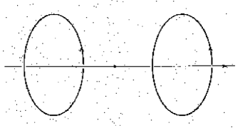
The two circles are where , while the line linking them is where . The arrows on the curves serve partly to distinguish solitons from anti-solitons: the convention here is that solitons obey the right-hand rule, whereas anti-solitons would obey the left-hand rule.
Let denote the angle between and (ie the pair is rotated by about the line joining the two solitons). Let denote the energy of a single soliton, and the energy of the two-soliton system, as a function of the separation and the relative phase . Considering the potential energy of the interacting dipoles suggests that
| (7) |
for some constant . Clearly is minimized, for a given , when (ie when the two solitons are in phase): this is channel . The formula (7) was tested numerically, by computing the energy of the configurations obtained by combining translated and rotated versions of the approximate one-soliton (3). The combination anstaz was simply that of addition (), which is a plausible approximation for large (bearing in mind that the -field tends to zero away from each soliton). For in the range , the form (7) is indeed found to hold, with . (In view of the crudity of the “sum” ansatz, the accuracy is not claimed to be better than 10% or so; but the dependence is very clear.) The behaviour under the discrete symmetries is the same as for the 1-soliton, namely .
Channel B.
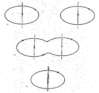
This channel is one in which both dipole pairs are co-planar with , with and being parallel (and orthogonal to ). This configuration is depicted in Fig 2(a).
In this case, the effect of the discrete symmetries on the configuration is . Consideration of the forces between the dipoles suggests that the energy behaves like
| (8) |
where is the angle that makes with . The expression (8) has a minimum when , and this is attractive channel .
Channel C.
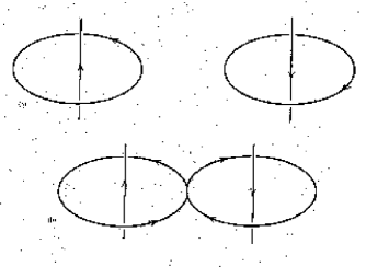
Here the dipole pairs are again co-planar with , but now and are anti-parallel. This is depicted in Fig 3(a).
In this case, one expects that
| (9) |
where, as before, is the angle that makes with . So the attractive force is maximal when . The dependence (9) was confirmed numerically, as before, with . This ‘maximally-attractive’ channel is referred to as channel . The effect of the discrete symmetries is , as for channel .
4 Relaxing in Channel A
In this section, we see what happens when we begin with two solitons far apart (in the first of the attractive channels described above), and minimize the energy. This was done numerically, using a conjugate-gradient procedure.
Suppose, then, that we start in the (axisymmetric) channel , and minimize energy without breaking the axial symmetry. Then the two solitons approach each other along the line joining them, and the minimum is reached when they are a nonzero distance apart. The resulting configuration therefore is a static solution of the field equation; it has energy (this is to be compared with ), and it resembles two rings around the -axis, separated by a distance . In other words, consists of the -axis plus infinity, as for the 1-soliton, while consists of two disjoint rings around it; so the linking number does indeed equal 2. The picture is as in Fig 1.
There is an approximate configuration analogous to (3), namely
| (10) |
where and are parameters, and are cubic polynomials, and . The two-ring structure is evident from (10). Minimizing the energy of (10) with respect to the ten parameters (, , and the coefficients of and ) gives an energy , it ie above that of the solution. The corresponding configuration is very close to the actual solution.
While this is a solution, it is not the global minimum of the energy in the sector; in particular, channel produces a solution with lower energy. So the question arises as to whether the channel minimum is stable to (non-axisymmetric) perturbations (ie whether it is a local minimum of the energy, as opposed to a saddle-point). The linking behaviour of the channel minimum is that of a single ring around a double axis (as we shall see in the next section), as opposed to a double ring around a single axis; there is a continuous path in configuration space from the one configuration to the other, but the contortions involved in this suggest that there is an energy barrier (in other words, that the channel solution is a local minimum). Numerical experiments, involving random perturbations of this solution, provide strong support for this; but more study is needed.
5 Relaxing in Channel B
Next, we start in channel and once again flow down the energy gradient. As depicted in Fig 2, the two rings (where ) merge into one, and then the two lines where merge as well. We end up with a solution which has been described previously [7], [9], [10], and which is believed to be the global minimum in the sector. It is axially-symmetric, and resembles a single ring; but this time the ring winds around a double copy of the -axis, and hence it has a linking number of . The energy of the solution is , which agrees with the figure given in [7].
As before, we can write down an explicit configuration which is very close to the solution. One such expression is
| (11) |
where is a constant and is a quintic polynomial. Minimizing the energy with respect to the six coefficients contained in (11) gives (ie above the true minimum), for
| (12) |
Since has only one positive root, is a ring (of radius ) in the -plane; whereas is the -axis, with multiplicity two. The components of derived from (11) are very close to those of the actual solution.
6 Relaxing in Channel C
If one begins with the configuration depicted in Fig 3(a) and moves in the direction of the energy gradient, the two solitons approach each other. If the two loops touch, one has a figure-eight curve, with the lines linking through it in opposite directions: Fig 3(b). This configuration is certainly not stable: preliminary numerical work indicates that the two ‘halves’ of the configuration rotate by (in opposite directions) about the axis joining them. So the figure-eight untwists to become a simple loop, and the two curves end up pointing in the same direction, exactly as in Fig 2(b) and (c). Hence the minimum in channel is the same as that in channel . Between this mimimum and the channel- one, there should be saddle-point solutions; but what these look like is not yet clear.
7 Concluding Remarks
There has already been some study of two-soliton dynamics, using a “direct” numerical approach (see, for example, [11]); this is computationally very intensive. The results reported in this Letter could be viewed as the first step towards a somewhat different approach, namely that of constructing a collective-coordinate manifold for the two-soliton system. The analogous structure for the Skyrme model has been investigated in some detail [15], [16]; in particular, it has the advantage that one can introduce quantum corrections by quantizing the dynamics on the collective-coordinate manifold [17]. Since each Hopf soliton depends on six parameters, the two-soliton manifold should have dimension (at least) twelve; each point of corresponds to a relevant configuration, and the expressions (3) and (11) are examples of such configurations.
But clearly much more work remains to be done towards understanding the energy functional on the configuration space. The suggestion of this Letter is that the global minimum (which is, of course, degenerate: it depends on six moduli) is as in Fig 2(c); there is a local minimum as in Fig 1; and between the two are saddle-point solutions which may be related to the figure-eight configuration Fig 3(b).
References
- [1] L Faddeev, A J Niemi, Phys Rev Lett 82 (1999) 1624; hep-th/9807069
- [2] S V Shabanov, Phys Lett B 458 (1999) 322.
- [3] Y M Cho, H W Lee, D G Pak, Effective Theory of QCD, hep-th/9905215
- [4] L Faddeev, Quantisation of Solitons [Preprint IAS Print-75-QS70, Princeton]; Lett Math Phys 1 (1976) 289.
- [5] H J deVega, Phys Rev D 18 (1978) 2945.
- [6] L Faddeev, A J Niemi, Nature 387 (1997) 58.
- [7] J Gladikowski, M Hellmund, Phys Rev D 56 (1997) 5194
- [8] R A Battye, P M Sutcliffe, Solitonic Strings and Knots. To appear in the CRM Series in Mathematical Physics (Springer-Verlag).
- [9] R A Battye, P M Sutcliffe, Phys Rev Lett 81 (1998) 4798; hep-th/9808129
- [10] R A Battye, P M Sutcliffe, Proc R Soc Lond A 455 (1999) 4305; hep-th/9811077
- [11] J Hietarinta, P Salo P, Phys Lett B 451 (1999) 60; hep-th/9811053
- [12] R S Ward, Nonlinearity 12 (1999) 1; hep-th/9811176
- [13] T R Govindarajan, Mod Phys Lett A 13 (1998) 3179; hep-th/9811171
- [14] A J Niemi, Knots in Interaction, hep-th/9902140
- [15] N S Manton, Phys Rev Lett 60 (1988) 1916.
- [16] M F Atiyah, N S Manton, Commun Math Phys 152 (1993) 391.
- [17] R A Leese, N S Manton, B J Schroers, Nucl Phys B 442 (1995) 228.