Abstract

Liouville conformal field theory is considered with conformal boundary. There is a family of conformal boundary conditions parameterized by the boundary cosmological constant, so that observables depend on the dimensional ratios of boundary and bulk cosmological constants. The disk geometry is considered. We present an explicit expression for the expectation value of a bulk operator inside the disk and for the two-point function of boundary operators. We comment also on the properties of the degenrate boundary operators. Possible applications and further developments are discussed. In particular, we present exact expectation values of the boundary operators in the boundary sin-Gordon model.

1 Liouville field theory

During last 20 years the Liouvlle field theory permanently attracts much attention mainly due to its relevance in the quantization of strings in non-critical space-time dimensions [1] (see also refs.[2, 3, 4]). It is also applied as a field theory of the 2D quantum gravity. E.g., the results of the Liouville field theory (LFT) approach can be compared with the calculations in the matrix models of two-dimensional gravity [5, 6] and this comparison shows [7, 8] that when the LFT central charge $c_{L}\geq 25$ this field theory describes the same continuous gravity as was found in the critical region of the matrix models. Although there are still no known applications of LFT with $c_{L}<25$, the theory is interesting on its own footing as an example of non-rational 2D conformal field theory.

In the bulk the Liouville field theory is defined by the Lagrangian density

$${\mathcal{L}}=\frac{1}{4\pi}(\partial_{a}\phi)^{2}+\mu e^{2b\phi}$$ (1.1)

where $\phi$ is the two-dimenesional scalar field, $b$ is the dimensionless Liouville coupling constant and the scale parameter $\mu$ is called the cosmological constant. This expression implies a trivial background metric $g_{ab}=\delta_{ab}$. In more general background the action reads

$$A_{\mathrm{bulk}}=\frac{1}{4\pi}\int\limits_{\Gamma}\left[g^{ab}\partial_{a}\phi\partial_{b}\phi+QR\phi+4\pi\mu e^{2b\phi}\right]\sqrt{g}d^{2}x$$ (1.2)

Here $R$ is the scalar curvature associated with the background metric $g$ while $Q$ is an important quantity in the Liouville field theory called the background charge

$$Q=b+1/b$$ (1.3)

It determines in particular the central charge of the theory

$$c_{L}=1+6Q^{2}$$ (1.4)

In what follows we always will consider only the simplest topologies like sphere or disk which can be described by a trivial background. For example, a sphere can be represented as a flat projective plane where the flat Liouville lagrangian (1.1) is valid if we put away all the curvature to the spacial infinity where it is seen as a special boundary condition on the Liouville field $\phi$

$$\phi(z,\bar{z})=-Q\log(z\bar{z})+O(1)\ \ \ \ \ \mathrm{at}\ \ |z|\rightarrow\infty$$ (1.5)

called the background charge at infinity.

The basic objects of LFT are the exponential fields $V_{\alpha}(x)=\exp(2\alpha\phi(x))$ which are conformal primaries w.r.t. the stress tensor

$$T(z{)} {}=-(\partial\phi)^{2}+Q\partial^{2}\phi$$ (1.6)

$$\bar{T}(\bar{z}{)} {}=-(\bar{\partial}\phi)^{2}+Q\bar{\partial}^{2}\phi$$

The field $V_{\alpha}$ has the dimension

$$\Delta_{\alpha}=\alpha(Q-\alpha)$$ (1.7)

In fact not all of these operators are independent. One has to identify the operators $V_{\alpha}$ and $V_{Q-\alpha}$ so that the whole set of local LFT fields is obtained by the “folding” of the complex $\alpha$-plane w.r.t. this reflection. The only exception is the line $\alpha=Q/2+iP$ with $P$ real where these exponential fields, if interpreted in terms of quantum gravity, seem not to correspond to local operators. E.g. in the classical theory they appear as hyperbolic solutions to the Lioville equation and “create holes” in the surface [9, 10]. Instead, these values of $\alpha$ are attributed to the normalizable states. The LFT space of states $\mathcal{A}$ consists of all conformal families $[v_{P}]$ corresponding to the primary states $\left|v_{P}\right\rangle$ with real $0\leq P<\infty$, i.e.,

$${\mathcal{A}}=\bigotimes_{P\in[0,\infty)}[v_{P}]$$ (1.8)

The primary states $\left|v_{P}\right\rangle$ are related to the values $\alpha=Q/2+iP$ and have dimensions $Q^{2}/4+P^{2}$ while other values of $\alpha$ are mapped onto non-normalizable states. This is a peculiarity of the operator-state correspondence of the Liouville field theory which differs it from conventional CFT with discret spectra of dimensions but make it similar to some conformal $\sigma$-models with non-compact target spaces. In what follows the primary physical states are normalized as

$$\left\langle v_{P^{\prime}}|v_{P}\right\rangle=\pi\delta(P-P^{\prime})$$ (1.9)

The solution of the spherical LFT amounts to constructing all multipoint correlation functions of these fields,

$$G_{\alpha_{1\ldots}\alpha_{N}}(x_{1},\ldots,x_{N})=\left\langle V_{\alpha_{1}}(x_{1})\ldots V_{\alpha_{N}}(x_{N})\right\rangle$$ (1.10)

In principle these quantities are completely determined by the structure of the operator product expansion (OPE) algebra of the exponential operators, i.e. can be completely restored from the two-point function

$$\left\langle V_{a}(x)V_{a}(0)\right\rangle=\frac{D(\alpha)}{(x\bar{x})^{2\Delta_{\alpha}}}$$ (1.11)

which determines the normalization of the basic operators and the three-point function

$$G_{\alpha_{1},\alpha_{2},\alpha_{3}}(x_{1},x_{2},x_{3})=\left|x_{12}\right|^{2\gamma_{3}}\left|x_{23}\right|^{2\gamma_{1}}\left|x_{31}\right|^{2\gamma_{2}}C(\alpha_{1},\alpha_{2},\alpha_{3})$$ (1.12)

with $\gamma_{1}=\Delta_{\alpha_{1}}-\Delta_{\alpha_{2}}-\Delta_{\alpha_{3}}$, $\gamma_{2}=\Delta_{\alpha_{2}}-\Delta_{\alpha_{3}}-\Delta_{\alpha_{1}}$, $\gamma_{3}=\Delta_{\alpha_{3}}-\Delta_{\alpha_{1}}-\Delta_{\alpha_{2}}$ . Once these quantities are known, the multipoint functions can be in principle reconstructed by the purely “kinematic” calculations relied on the conformal symmetry only. Although these calculations present a separate rather complicated technical problem, conceptually one can say that a CFT (on a sphere) is constructed if these basic objects are found.

For LFT these quantities were first obtained by Dorn and Otto[11, 12] in 1992 (see also [13]). We will present here the derivation of the simplest of them, the two-point function $D(\alpha)$, to illustrate a different approach to this problem proposed more recently by J.Techner [14] which seems more effecticient. Close ideas are also developed in the studies of LFT by Gervais and collaborators [15]. We will use similar approach shortly in the discussion of the boundary Liouville problem.

Among the exponential operators $V_{\alpha}$ there is a series of fields $V_{-nb/2}$, $n=0,1,\ldots$ which are degenerate w.r.t. the conformal symmetry algebra and therefore satisfy certain linear differential equations. For example, the first non-trivial operator $V_{-b/2}$ satisfies the following second order equation

$$\left(\frac{1}{b^{2}}\partial^{2}+T(z)\right)V_{-b/2}=0$$ (1.13)

and the same with the complex conjugate differentiation in $\bar{z}$ and $\bar{T}(\bar{z})$ instead of $T$. In the classical limit of LFT the existence of this degenerate operator can be traced back to the well known relation between the ordinary second-order linear differential equation and the classical partial-derivative Liouville equation [16]. The next operator $V_{-b}$ satisfies two complex conjugate third-order differential equations

$$\left(\frac{1}{2b^{2}}\partial^{3}+2T(z)\partial+(1+2b^{2})\partial T(z)\right)V_{-b}=0$$ (1.14)

and so on. It follows from these equations that the operator product expansion of these degenerate operators with any primary field, in the present case with our basic exponential fields $V_{\alpha}$, is of very special form and contains in the r.h.s only finite number of primary fields. For example for the first one there are only two representations

$$V_{-b/2}V_{\alpha}=C_{+}\left[V_{\alpha-b/2}\right]+C_{-}\left[V_{\alpha+b/2}\right]$$ (1.15)

where $C_{\pm}$ are the special structure constants. What is important to remark about these special structure constants is that the general CFT and Coulomb gas experience suggests that they can be considered as “perturbative”, i.e. are obtained as certain Coulomb gas (or “screening”) integrals [17, 18]. For example in our case in the first term of (1.15) there is no need of screening insertion and therefore one can set $C_{+}=1$. The second term requires a first order insertion of the Liouville interaction $-\mu\int\exp(2b\phi)d^{2}x$ and

$$C_{-} =-\mu\int d^{2}x\left\langle V_{\alpha}(0)V_{-b/2}(1)e^{2b\phi(x)}V_{Q-\alpha-b/2}(\infty)\right\rangle$$

$$=-\mu\dfrac{\pi\gamma(2b\alpha-1-b^{2})}{\gamma(-b^{2})\gamma(2b\alpha)}$$ (1.16)

where as usual $\gamma(x)=\Gamma(x)/\Gamma(1-x)$. It is remarkable that all the special structure constants entering the special truncated OPE’s with the degenerate fields can be obtained in this way.

Now let us take the two-point function $D(\alpha)$ and consider the auxiliary three-point function

$$\left\langle V_{\alpha}(x_{1})V_{\alpha+b/2}(x_{2})V_{-b/2}(z)\right\rangle$$

Then, tending $z\rightarrow x_{1}$ we see that in the OPE only the second term survives and in fact our auxiliary function is $\sim C_{-}D(\alpha+b/2)$. Instead tending $z\rightarrow x_{2}$ we can “lower” the parameter of the second operator down to $\alpha$ which results in $C_{+}D(\alpha)$. Equating these two things we arrive at the functional equation for the two-point function

$$\frac{D(\alpha+b/2)}{D(\alpha)}=C_{-}^{-1}(\alpha)$$ (1.17)

This equation can be easily solved in terms of gamma-functions

$$D(\alpha)=\left(\pi\mu\gamma(b^{2})\right)^{(Q-2\alpha)/b}\frac{\gamma(2b\alpha-b^{2})}{b^{2}\gamma(2-2\alpha/b+1/b^{2})}$$ (1.18)

which coincides precisely with what was obtained for this quantity in the original studies.

In fact there are many solutions to the above functional equation. It is relevant for the moment to stop at the remarkable duality property of LFT. Besides the abovementioned series of degenerate operators $V_{-nb/2}$ there is a “dual” series with $b$ replaced by $1/b$. This results in another “dual” functional equation for $D(\alpha)$ with the shift by $1/b$ instead of $b$. The solution becomes unique (at least if these two shifts are uncomparable) [14]. Note that these two equations are compatible only if in the dual equation the cosmological constant $\mu$ is replaced by the “dual cosmological constant” $\tilde{\mu}$ related to $\mu$ as follows

$$\pi\tilde{\mu}\gamma(1/b^{2})=\left(\pi\mu\gamma(b^{2})\right)^{1/b^{2}}$$ (1.19)

With this definition of $\tilde{\mu}$ the duality property, which turn out to hold exactly in LFT, can be formulated as the symmetry of all observables w.r.t. the substitution $b\rightarrow 1/b$ and $\mu\rightarrow\tilde{\mu}$.

The same way one can readily obtain and solve the functional equations for the three-point function [14] which reads

$${C}(\alpha_{1},\alpha_{2},\alpha_{3})=\left[\pi\mu\gamma(b^{2})b^{2-2b^{2}}\right]{{}^{(Q-\sum\alpha_{i})/b}\times}$$ (1.20)

$$\ \ \frac{\Upsilon_{0}\Upsilon(2\alpha_{1})\Upsilon(2\alpha_{2})\Upsilon(2\alpha_{3})}{\Upsilon(\alpha_{1}+\alpha_{2}+\alpha_{3}-Q)\Upsilon(\alpha_{1}+\alpha_{2}-\alpha_{3})\Upsilon(\alpha_{2}+\alpha_{3}-\alpha_{1})\Upsilon(\alpha_{3}+\alpha_{1}-\alpha_{2})}$$

where a special function $\Upsilon(x)$ has to be introduced

$$\log\Upsilon(x)=\int_{0}^{\infty}\frac{dt}{t}\left[\left(Q/2-x\right)^{2}e^{-2t}-\frac{\sinh^{2}\left(Q/2-x\right)t}{\sinh(bt)\sinh(t/b)}\right]$$ (1.21)

This integral representation is convergent only in the strip $0<\mathrm{Re}$ $x<Q$, otherwise it is an analytic continuation. In fact $\Upsilon(x)$ is an entire function of $x$ with zeroes at $x=-nb-m/b$ and $x=Q+nb+m/b$ with $n$ and $m$ non-negative integers.

In the sense mentioned above the explicit results (1.11) and (1.20) constitute the exact construction of the Liouville field theory on a sphere. For example, the four-point function can be explicitly expressed in terms of the three-point function

$$G_{\alpha_{1},\alpha_{2},\alpha_{3},\alpha_{4}}(x_{i})={\frac{1}{\pi}}\int\limits_{0}^{\infty}C(\alpha_{1},\alpha_{2},Q/2+iP)C(\alpha_{3},\alpha_{4},Q/2-iP)|{\mathbf{F}}(\Delta_{\alpha_{i}},\Delta,x_{i})|^{2}dP$$ (1.22)

where the intergration is over the variety of physical states $\left|v_{P}\right\rangle$ and ${\mathbf{F}}(\Delta_{\alpha_{i}},\Delta,x_{i})$ is the four-point conformal block, determined completely by the conformal symmetry [19]. In the four-point case, which we are considering now, the latter can be further reduced to a function of one variable, e.g.,

$${\mathbf{F}}(\Delta_{\alpha_{i}},\Delta,x_{i}) =$$ (1.23)

$$\ (x_{4}-x_{1})^{-2\Delta_{1}}(x_{4}-x_{2})^{\Delta_{1}+\Delta_{3}-\Delta_{2}-\Delta_{4}}(x_{4}-x_{3})^{\Delta_{1}+\Delta_{2}-\Delta_{3}-\Delta_{4}}(x_{3}-x_{2})^{\Delta_{4}-\Delta_{1}-\Delta_{2}-\Delta_{3}}\times$$

$$\ {\mathcal{F}}\left(\begin{array}[c]{cc}\alpha_{1}&\alpha_{3}\\ \alpha_{2}&\alpha_{4}\end{array}\mid P\mid\eta\right)$$ (1.26)

where

$$\eta=\frac{(x_{1}-x_{2})(x_{3}-x_{4})}{(x_{1}-x_{4})(x_{3}-x_{2})}$$

Parameters $\alpha_{i}$ are related to $\Delta_{\alpha_{i}}$ as in eq.(1.7) and in the intermediate dimension $\Delta=Q^{2}/4+P^{2}$.

2 The boundary Liouville problem

The basic ideas of 2D conformal field theory with conformally invariant boundary were developed long ago mostly by J.Cardy [20] who also applied them successfully to rational CFT’s, in particular to the minimal series [21, 22]. Here we’ll try to apply these ideas to the Liouville CFT with boundary.

A conformally invariant boundary condition in LFT can be introduced through the following boundary interaction

$$A_{\mathrm{bound}}=A_{\mathrm{bulk}}+\int\limits_{\partial\Gamma}\left(\frac{QK}{2\pi}\phi+\mu_{B}e^{b\phi}\right)g^{1/4}d\xi$$ (2.1)

where the integration in $\xi$ is along the boundary while $K$ is the curvature of the boundary in the background geometry $g$. In what follows we consider only the geometry of a disk which can be represented as a simply connected domain $\Gamma$ in the complex plane with a flat background metric $g_{ab}=\delta_{ab}$ inside. The action is simplified as

$$A_{\mathrm{bound}}=\int\limits_{\Gamma}\left(\frac{1}{4\pi}(\partial_{a}\phi)^{2}+\mu e^{2b\phi}\right)d^{2}x+\int\limits_{\partial\Gamma}\left(\frac{Qk}{2\pi}\phi+\mu_{B}e^{b\phi}\right)d\xi$$ (2.2)

where $k$ is the curvature of the boundary in the complex plane. Typically the most convenient domain is either a unit circle or the upper half-plane. In the last case the boundary $\partial\Gamma$ is the real axis and one can omit the term linear in $\phi$ in the boundary action (2.2). The price is again a “background charge at infinity”, i.e., the same boundary condition on the field $\phi$ at infinity in the upper half plane

$$\phi(z,\bar{z})=-Q\log(z\bar{z})+O(1)\ \ \ \ \ \mathrm{at}\ \ |z|\rightarrow\infty$$ (2.3)

as in the case of the sphere.

It seems natural to call the additional parameter $\mu_{B}$ the boundary cosmological constant. We see that in fact there is a one-parameter family of conformally invariant boundary conditions characterized by different values of the boundary cosmological constant $\mu_{B}$. Contrary to the pure bulk situation where the cosmological constant enters only as a scale parameter, the observables in the boundary case actually depend on the scale invariant ratio $\mu/\mu_{B}^{2}$. For example, a disk correlation function with the bulk operators $V_{\alpha_{1}},V_{\alpha_{2}}\cdots V_{\alpha_{n}}$ and the boundary operators (see below) $B_{\beta_{1}},B_{\beta_{2}}\cdots B_{\beta_{m}}$ scales as follows

$${\mathcal{G}}(\alpha_{1,}\cdots\alpha_{n},\beta_{1},\cdots\beta_{m})\sim\mu^{(Q-2\sum_{i}\alpha_{i}-\sum_{j}\beta_{j})/2b}F\left(\frac{\mu_{B}^{2}}{\mu}\right)$$ (2.4)

where $F$ is some scaling function and we indicate only the dependence on the scale parameters $\mu$ and $\mu_{B}$. Our present purpose is to study this dependence.

In the boundary case we have to introduce the boundary operators. In LFT the basic boundary primaries are again the exponential in $\phi$ boundary fields $B_{\beta}=\exp\beta\phi$. Their dimensions are

$$\Delta_{\beta}=\beta\left(Q-\beta\right)$$ (2.5)

To avoid any confusions we shall always use parameter $\alpha$ for the bulk exponentials and parameter $\beta$ in relation with the boundary operators. In general a boundary operator is not characterized completely by its dimension, because the conformal boundary conditions at both sides of the location of the boundary operator may be in general different. One has to specify which boundary condition it joins. Therefore in general we are talking about a juxtaposition boundary operator between, in our case, two boundary conditions with the parameters $\mu_{B_{1}}=\mu_{1}$ and $\mu_{B_{2}}=\mu_{2}$ and denote it $B_{\beta}^{\mu_{1}\mu_{2}}(x)$.

To define completely the boundary LFT on the disk, i.e, to be able to construct an arbitrary multipoint correlation function including bulk and boundary operators, we have to reveal few more basic objects in addition to the bulk two- and three-point functions (1.18) and (1.20) we already have.

1. First is the bulk one-point function (we imply almost constantly the upper half-plane geometry)

$$\left\langle V_{\alpha}(x)\right\rangle=\frac{U(\alpha|\mu_{B})}{\left|z-\bar{z}\right|^{2\Delta_{\alpha}}}$$ (2.6)

In fig.1a it is drawn however as the one-point function in the unit disk.

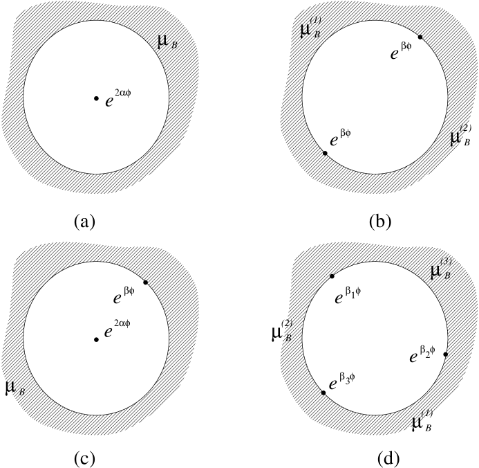
Figure 1:

2. Second, one needs the boundary two-point function

$$\left\langle B_{\beta}^{\mu_{1}\mu_{2}}(x)B_{\beta}^{\mu_{2}\mu_{1}}(0)\right\rangle=\frac{d(\beta|\mu_{1},\mu_{2})}{\left|x\right|^{2\Delta_{\beta}}}$$ (2.7)

which in general depends on two boundary cosmological constants $\mu_{1}$and $\mu_{2}$ (see fig.1b).

3. The bulk-boundary structure constant, which determines the fusion of a bulk operator $V_{\alpha}$ with the boundary resulting in the boundary operator $B_{\beta}^{\mu_{B}\mu_{B}}$. This is basically the same as the bulk-boundary two-point function (fig.1c)

$$\left\langle V_{\alpha}(z)B_{\beta}(x)\right\rangle=\frac{R(\alpha,\beta|\mu_{B})}{\left|z-\bar{z}\right|^{2\Delta_{\alpha}-\Delta_{\beta}}\left|z-x\right|^{2\Delta_{\beta}}}$$ (2.8)

In fact the one-point function (2.6) is a particular case of this quantity with $\beta=0$ so that its introduction, however convenient, is redundant.

4. Finally, there is a boundary three-point function

$$\left\langle B_{\beta_{1}}^{\mu_{2}\mu_{3}}(x_{1})B_{\beta_{2}}^{\mu_{3}\mu_{1}}(x_{2})B_{\beta_{3}}^{\mu_{1}\mu_{2}}(x_{3})\right\rangle=\frac{c(\beta_{1},\beta_{2},\beta_{3}|\mu_{1},\mu_{2},\mu_{3})}{\left|x_{12}\right|^{\Delta_{1}+\Delta_{2}-\Delta_{3}}\left|x_{23}\right|^{\Delta_{2}+\Delta_{3}-\Delta_{1}}\left|x_{31}\right|^{\Delta_{3}+\Delta_{1}-\Delta_{2}}}$$ (2.9)

which in fact depends now on three different boundary parameters, $\mu_{1}$, $\mu_{2}$ and $\mu_{3}$ related to the corresponding sides of the triangle as shown in fig.1d.

These three basic boundary structure constants, together with the bulk structure constants, allow in principle to write down an intermediate state expansions for any multipoint function. An instructive example is the bulk two-point function

$$G_{\alpha_{1}\alpha_{2}}(z_{1},z_{2})=\left\langle V_{\alpha_{1}}(z_{1})V_{\alpha_{2}}(z_{2})\right\rangle$$ (2.10)

Joining these two operators together with the bulk structure constant we can reduce this quantity to the one-point bulk function and write down the following expansion

$$G_{\alpha_{1}\alpha_{2}}=\frac{\left|z_{2}-\bar{z}_{2}\right|^{2\Delta_{1}-2\Delta_{2}}}{\left|z_{1}-\bar{z}_{2}\right|^{4\Delta_{1}}}\int\frac{dP}{\pi}C(\alpha_{1},\alpha_{2},Q/2+iP)\,\,U(Q/2-iP){\mathcal{F}}\left(\begin{array}[c]{cc}\alpha_{1}&\alpha_{1}\\ \alpha_{2}&\alpha_{2}\end{array}\left|P\right|\eta\right)$$ (2.11)

where

$$\eta=\frac{(z_{1}-z_{2})(\bar{z}_{1}-\bar{z}_{2})}{(z_{1}-\bar{z}_{2})(\bar{z}_{1}-z_{2})}$$ (2.12)

is the projective invariant of the four points $z_{1}$, $z_{2}$, $\bar{z}_{1}$ and $\bar{z}_{2}$ and $\mathcal{F}$ is the same four-point conformal block as enters the expansion of the four-point bulk function, see (1.22,1.23). Notice that while in that case it entered in a sesquilinear combination (1.22), here it appears linearly (J.Cardy [21]). Expansion (2.11) is suitable appropriate if the bulk operators are close to each other, i.e., $\eta\rightarrow 0$. Another representation is suitable the limit $\eta\rightarrow 1$ where the points $z_{1}$ and $z_{2}$ approach boundary and the bulk operators can be expanded in the boundary ones. This gives

$$G_{\alpha_{1}\alpha_{2}}=\frac{\left|z_{2}-\bar{z}_{2}\right|^{2\Delta_{1}-2\Delta_{2}}}{\left|z_{1}-\bar{z}_{2}\right|^{4\Delta_{1}}}\int\frac{dP}{\pi}R(\alpha_{1},Q/2+iP)R(\alpha_{2},Q/2-iP)\,{\mathcal{F}}\left(\begin{array}[c]{cc}\alpha_{1}&\alpha_{2}\\ \alpha_{1}&\alpha_{2}\end{array}\left|P\right|1-\eta\right)$$ (2.13)

Equating these two expressions we see that the basic boundary quantities also must satisfy some bootstrap relations analogous to that in the bulk case. It is interesting to note, that there is another application of this relation. The conformal block itself, although being completely determined by the conformal symmetry, is it fact a complicated function which is not in general known explicitly. On the other hand it is important since it explicitely enters the conformal bootstrap equations [19]. Besides, one might expect that it encodes some information about the structure of the representations of the conformal symmetry. In particular conformal block must satisfy the following cross-relation

$${\mathcal{F}}\left(\begin{array}[c]{cc}\alpha_{1}&\alpha_{3}\\ \alpha_{2}&\alpha_{4}\end{array}\left|P\right|\eta\right)=\int\frac{dP^{\prime}}{2\pi}K\left(\begin{array}[c]{cc}\alpha_{1}&\alpha_{3}\\ \alpha_{2}&\alpha_{4}\end{array}\mid P,P^{\prime}\right)\,{\mathcal{F}}\left(\begin{array}[c]{cc}\alpha_{1}&\alpha_{2}\\ \alpha_{3}&\alpha_{4}\end{array}\left|P^{\prime}\right|1-\eta\right)$$ (2.14)

with some cross-matrix $K$ which determines the monodromy properties of the conformal block. Suppose now we’ve managed to find the basic quantities of the boundary Liouville problem, in particular the one-point function $U(\alpha)$ and the bulk-boundary structure constant $R(\alpha,\beta)$. Then the crossing relation becomes a linear equation for the cross-matrix of the symmetric (i.e., $\alpha_{3}=\alpha_{1}$ and $\alpha_{4}=\alpha_{2}$) conformal block, from where this matrix can be figured out.

2.1 Bulk one-point function

We start with the calculation of the bulk one point function $U(\alpha|\mu_{B})$. For this we apply the degenerate operator insertion, like above for the bulk two-point function. Consider the auxiliary bulk two-point function with the additional degenerate bulk field $V_{-b/2}(z)$

$$G_{\alpha,-b/2}(x,z)=\left\langle V_{\alpha}(x)V_{-b/2}(z)\right\rangle$$ (2.15)

Apply first the OPE at $z\rightarrow x$ where the degenerate operator $V_{-b/2}$ generates only two primary fields so that

$$G_{\alpha,-b/2}=C_{+}\,(\alpha)U(\alpha-b/2){\mathcal{G}}_{+}(x,z)+C_{-}(\alpha)\,\,U(\alpha+b/2){\mathcal{G}}_{-}(x,z)$$ (2.16)

where $C_{\pm}(\alpha)$ are the special structure constants as given by the screening integrals and ${\mathcal{G}}_{\pm}(x,z)$ are expressed through the special conformal blocks ${\mathcal{F}}_{\pm}(x,z)$ related to these special values of parameters

$${\mathcal{G}}_{\pm}(x,z)=\frac{\left|x-\bar{x}\right|^{2\Delta_{\alpha}-2\Delta_{-b/2}}}{\left|z-\bar{x}\right|^{4\Delta_{\alpha}}}{\mathcal{F}}_{\pm}(\eta)$$ (2.17)

where $\Delta_{-b/2}=-1/2-3b^{2}/4$ and

$$\eta=\frac{(z-x)(\bar{z}-\bar{x})}{(z-\bar{x})(\bar{z}-x)}$$ (2.18)

In fact $V_{-b/2}$ satisfies the second order differential equation. Therefore these special conformal blocks are solution to a second order linear differential equation and can be expressed in terms of the hypergeometric functions

$${\mathcal{F}}_{+}(\eta)= {\mathcal{F}}\left(\begin{array}[c]{cc}-b/2&-b/2\\ \alpha&\alpha\end{array}|\alpha-\frac{b}{2}|\eta\right)=$$ (2.21)

$$\ \eta^{\alpha b}(1-\eta)^{-b^{2}/2}F(2\alpha b-1-2b^{2},-b^{2},2\alpha b-b^{2},\eta)$$ (2.22)

$${\mathcal{F}}_{-}(\eta)= {\mathcal{F}}\left(\begin{array}[c]{cc}-b/2&-b/2\\ \alpha&\alpha\end{array}|\alpha+\frac{b}{2}|\eta\right)=$$ (2.25)

$$\ \eta^{1+b^{2}-\alpha b}(1-\eta)^{-b^{2}/2}F(-b^{2},1-2\alpha b,2+b^{2}-2\alpha b,\eta)$$

This is a particular case of more general conformal block with a degenerate operator $V_{-b/2}$

$${\mathcal{F}}\left(\begin{array}[c]{cc}-b/2&\alpha_{3}\\ \alpha_{2}&\alpha_{4}\end{array}|\alpha_{2}-\frac{b}{2}|\eta\right) =\eta^{b\alpha_{2}}(1-\eta)^{\alpha_{3}b}F(A,B,C,\eta)$$ (2.28)

$${\mathcal{F}}\left(\begin{array}[c]{cc}-b/2&\alpha_{3}\\ \alpha_{2}&\alpha_{4}\end{array}|\alpha_{2}+\frac{b}{2}|\eta\right) =\eta^{1+b^{2}-b\alpha_{2}}(1-\eta)^{b\alpha_{3}}F(A-C+1,B-C+1,2-C,\eta)$$ (2.31)

where

$$A =-1+b(\alpha_{2}+\alpha_{3}+\alpha_{4}-3b/2)$$

$$B =b(\alpha_{2}+\alpha_{3}-\alpha_{4}-b/2)$$ (2.32)

$$C =b(2\alpha_{2}-b)$$

Now, as both operators approach the boundary, they are expanded in the boundary operators. It turns out that the degenerate bulk operator $V_{-b/2}$ near the boundary gives rise to only two primary boundary families $B_{0}$ and $B_{-b}$. The simplest thing is to find the contribution of $B_{0}=I$. The fusion of $V_{\alpha}$ to the unity boundary operator is described by the quantity $R(\alpha,0)=v(\alpha)$ while the fusion of the field $V_{-b/2}$ ($V_{-b/2}\rightarrow$ boundary) is described by a special bulk-boundary structure constant $R(-b/2,Q).$ It can be computed as the following boundary screening integral with one insertion of the boundary interaction $-\mu_{B}\int B_{b}(x)dx$

$$R(-b/2,Q) =-2^{2\Delta_{12}}\mu_{B}\int\left\langle V_{-b/2}(i)B_{b}(x)B_{Q}(\infty)\right\rangle dx$$ (2.33)

$$=-\frac{2\pi\mu_{B}\Gamma(-1-2b^{2})}{\Gamma^{2}(-b^{2})}$$

Comparing this with the behavior predicted by the bulk expansion (2.16) we find the following functional equation for the one-point function

$$-\frac{2\pi\mu_{B}}{\Gamma(-b^{2})}U(\alpha)=\frac{\Gamma(-b^{2}+2b\alpha)}{\Gamma(-1-2b^{2}+2b\alpha)}U(\alpha-b/2)-\frac{\pi\mu\Gamma(-1-b^{2}+2b\alpha)}{\gamma(-b^{2})\Gamma(2b\alpha)}U(\alpha+b/2)$$ (2.34)

(in the last term we used the bulk special structure constant $C_{-}(\alpha)$ from(1.16)). Equation is solved by the following simple expression

$$U(\alpha)=\frac{2}{b}\left(\pi\mu\gamma(b^{2})\right)^{(Q-2\alpha)/2b}\Gamma(2b\alpha-b^{2})\Gamma\left(\frac{2\alpha}{b}-\frac{1}{b^{2}}-1\right)\cosh(2\alpha-Q)\pi s$$ (2.35)

where the parameter $s$ is related to the scale invariant ratio of the cosmological constants

$$\cosh^{2}\pi bs=\frac{\mu_{B}^{2}}{\mu}\sin\pi b^{2}$$ (2.36)

Also this expression satisfies the dual functional equation provided the dual bulk cosmological constant $\tilde{\mu}$ is related to $\mu$ as before in (1.19) while the parameter $s$ is self-dual, i.e. the dual boundary cosmological constant $\tilde{\mu}_{B}$ is defined as follows

$$\cosh^{2}\frac{\pi s}{b}=\frac{\tilde{\mu}_{B}^{2}}{\tilde{\mu}}\sin\frac{\pi}{b^{2}}$$ (2.37)

It is remarkable enough that the expression (2.35) automatically satisfies the “reflection relation” [13] for the operator $V_{\alpha}$

$$U(\alpha)=U(Q-\alpha)D(\alpha)$$ (2.38)

with the bulk Liouville two-point function (1.18). If $\alpha$ corresponds to a physical state, i.e., $\alpha=Q/2+iP$ with $P$ real, expression (2.35) reads

$$U(P)=\left(\pi\mu\gamma(b^{2})\right)^{-iP/b}\Gamma\left(1+2ibP\right)\Gamma\left(1+2iP/b\right)\frac{\cos\left(2\pi sP\right)}{iP}$$ (2.39)

This quantity is interpreted as the matrix element between a primary physical state $\left|v_{P}\right\rangle$ from (1.8) and the boundary state $\left\langle B_{s}\right|$ created by the boundary action (2.2)

$$U(P)=\left\langle B_{s}|v_{P}\right\rangle$$ (2.40)

It is natural that this matrix element satisfies the reflection relation

$$U(P)=S(P)U(-P)$$ (2.41)

with the Liouville reflection amplitude [13]

$$S_{\mathrm{L}}(P)=-\left(\pi\mu\gamma(b^{2})\right)^{-2iP/b}\frac{\Gamma(1+2iP/b)\Gamma(1+2iPb)}{\Gamma(1-2iP/b)\Gamma(1-2iPb)}$$ (2.42)

Of course the functional relation does not fix the overall constant so that it can be multiplied by any (self-dual) factor $U_{0}(b)=U_{0}(1/b)$. In (2.35) this factor is chosen in the way that all the residues in the “on-mass-shell” poles at $2\alpha=Q-nb$, with $n=1,2,3,\ldots$ are equal precisely to the corresponding perturbative integrals appearing in expansions in $\mu$ and $\mu_{B}$, i.e.

$${{\operatorname*{res}}_{2\alpha=Q-nb}} \frac{U(\alpha)}{2^{2\Delta_{\alpha}}}=\sum\limits_{k=0}^{[n/2]}\frac{(-\mu)^{k}(-\mu_{B})^{n-2k}}{k!(n-2k)!}\times$$ (2.43)

$$\ \int\limits_{\mathrm{Im}z_{i}>0}d^{2}z_{1}\ldots d^{2}z_{k}\int\limits_{-\infty}^{\infty}dx_{1}\ldots dx_{n-2k}\left\langle V_{Q-nb}(i)V_{b}(z_{1})\ldots V_{b}(z_{k})B_{b}(x_{1})\ldots B_{b}(x_{n-2k})\right\rangle_{0}$$

where $\left\langle\cdots\right\rangle_{0}$ is the correlation function w.r.t the upper half plane free field with $\mu=\mu_{B}=0$ i.e., with free boundary conditions. Explicitely

$$\left\langle V_{\alpha_{1}}(z_{1})\ldots V_{\alpha_{n}}(z_{n})B_{\beta_{1}}(x_{1})\ldots B_{\beta_{m}}(x_{m})\right\rangle_{0}=\frac{\prod\limits_{i=1}^{n}\left|z_{i}-\bar{z}_{i}\right|^{-2\alpha_{i}^{2}}\prod\limits_{i,j}\left|z_{i}-x_{j}\right|^{-4\alpha_{i}\beta_{j}}}{\prod\limits_{i>j}^{m}\left|x_{i}-x_{j}\right|^{2\beta_{i}\beta_{j}}\prod\limits_{i>j}^{n}\left|(z_{i}-z_{j})(z_{i}-\bar{z}_{j})\right|^{4\alpha_{i}\alpha_{j}}}$$ (2.44)

In particular, the pure boundary perturbations in $\mu_{B}$ reproduce the Dyson integrals over a unit circle

$$\oint\frac{\prod_{i}^{n}du_{i}}{\prod_{i>j}^{n}\left|u_{i}-u_{j}\right|^{2b^{2}}}=\left(\frac{2\pi}{\Gamma(1-b^{2})}\right)^{n}\Gamma(1-nb^{2})$$ (2.45)

Several remarks are in order in connection with the expression (2.35) presented.

1. Semiclassical tests. Consider the limit $b\rightarrow 0$ while $P$ in eq.(2.39) is of order $b$ and $s$ is of order $b^{-1}$. In this limit the minisuperspace approximation is expected to work. Take the geometry of semi-infinite cylinder of circumference $2\pi$ and consider the states on the circle. In the minisuperspace approximation one takes into account the dynamics of the zero mode

$$\phi_{0}=\frac{1}{2\pi}\int_{0}^{2\pi}\phi(x)dx$$ (2.46)

neglecting completely all the oscillator modes of field $\phi(x)$. The primary state $\left|v_{P}\right\rangle$ is represented now by the wave function

$$\psi_{P}(\phi_{0})=\frac{2\left(\pi\mu/b^{2}\right)^{-iP/b}}{\Gamma\left(-2iP/b\right)}K_{2iP/b}\left(2\sqrt{\pi\mu/b^{2}}e^{b\phi_{0}}\right)$$ (2.47)

($K_{v}(z)$ is the modified Bessel function) which satisfies the minisuperspace Shrödinger equation

$$\left(-\frac{1}{2}\frac{d^{2}}{d\phi_{0}^{2}}+2\pi\mu e^{2b\phi_{0}}-2P^{2}\right)\psi_{P}(\phi_{0})=0$$ (2.48)

and has the following asymptotic at $\phi_{0}\rightarrow-\infty$

$$\psi_{P}(\phi_{0})=e^{2iP\phi_{0}}+S_{\text{{L}}}^{\mathrm{(cl)}}(P)e^{-2iP\phi_{0}}$$ (2.49)

where $S_{\text{{L}}}^{\mathrm{(cl)}}(P)$ is the classical limit of the Liouville reflection amplitude (2.42). Also it meets the normalization (1.9)

$$\int_{-\infty}^{\infty}\psi_{P^{\prime}}^{*}(\phi_{0})\psi_{P}(\phi_{0})=\pi\delta(P-P^{\prime})$$ (2.50)

In the approximation under consideration the boundary state $\left\langle B_{s}\right|$ wave function is simply related to the boundary Lagrangian

$$\Psi_{B_{s}}(\phi_{0})=\exp(-2\pi\mu_{B}e^{b\phi_{0}})$$ (2.51)

The matrix element $\left\langle B_{s}|v_{P}\right\rangle$ can be carried out explicitely

$$\int_{-\infty}^{\infty}\Psi_{B_{s}}(\phi_{0})\psi_{P}(\phi_{0})d\phi_{0}=\frac{2}{b}\left(\pi\mu/b^{2}\right)^{-iP/b}\Gamma\left(2iP/b\right)\cos(2\pi Ps)$$ (2.52)

and agrees precisely with the corresponding limit of (2.39). Note, that this calculation is sensitive to the prefactor in eq.(2.35) and confirms our choice $U_{0}(b)=1$, at least in the limit $b\rightarrow 0$.

2. Boundary length distribution. From the point of view of 2D gravity one can interprete the quantity

$$l=\int_{\partial\Gamma}\exp b\phi$$ (2.53)

as the lenth of the boundary. Let $W_{\alpha}(l)$ be the boundary length distribution for the fluctuating disk with the bulk cosmological constant $\mu$ and an insertion of the operator $V_{\alpha}$ somewhere inside the disk. Then

$$U(\alpha|\mu_{B})=\int_{0}^{\infty}\frac{dl}{l}e^{-\mu_{B}l}W_{\alpha}(l)$$ (2.54)

Form the result (2.35) one finds explicitely

$$W_{\alpha}(l)=\frac{2}{b}\left(\pi\mu\gamma(b^{2})\right)^{(Q-2\alpha)/2b}\frac{\Gamma(2\alpha b-b^{2})}{\Gamma(1+1/b^{2}-2\alpha/b)}K_{(Q-2\alpha)/b}(\kappa l)$$ (2.55)

where

$$\kappa^{2}=\frac{\mu}{\sin\pi b^{2}}$$ (2.56)

Compare (2.55) with the minisuperspace distribution (2.47). This result implies that the Shrödinger equation (2.48) in the logarithm of the scale $\phi_{0}=b^{-1}\log(l/2\pi)$ (which is called sometimes the Wheeler-deWitt equation) does not hold only in semiclassical limit but is in fact exact with a suitable renormalizations of constants (see in this relation the paper [24] where this equation first appeared in the context of the Liouville field theory, and also [25, 26] where similar expressions are obtained in the framework of random surface models).

Let us present also the double distribution in the length (2.53) and area $A$ defined as

$$W_{\alpha}(l,\mu)=\int_{0}^{\infty}\frac{dA}{A}e^{-\mu A}Z_{\alpha}(A,l)$$ (2.57)

It is given by a rather simple expression

$$Z_{\alpha}(A,l)=\frac{1}{b}\frac{\Gamma(2\alpha b-b^{2})}{\Gamma(1+1/b^{2}-2\alpha/b)}\left(\frac{l\Gamma(b^{2})}{2A}\right)^{(Q-2\alpha)/b}\exp\left(-\frac{l^{2}}{4A\sin\pi b^{2}}\right)$$ (2.58)

3. “Heavy” $\alpha$ semiclassics. Consider again the limit $b\rightarrow 0$ but with large value of $\alpha=\eta/b$ not nessesserily close to $Q/2$. Exact expression (2.58) gives in this limit

$$Z_{\eta/b}(A,l)=\frac{l\Gamma(2\eta)e^{(\eta-1/2)C}}{2b^{2}A\sqrt{2\pi(1-2\eta}}\exp\left(-\frac{1}{b^{2}}S_{\eta}(A,l)\right)$$ (2.59)

where $C$ is the Euler’s constant and

$$S_{\eta}(A,l)=\frac{l^{2}}{4\pi A}+(1-2\eta)\left(\log\left(2A/l\right)+\log(1-2\eta)-1\right)$$ (2.60)

On the other hand the corresponding classical solution with the area $A$ and the boundary lenght $l$ reads for the classical field $\varphi=2b\phi$ (we imply here the geometry of the disk $\left|z\right|\leq 1$ with the unit circle as the boundary)

$$e^{\varphi(z)}=\frac{l^{2}(a^{-1}-a)^{2}}{\left[2\pi(a^{-1}(z\bar{z})^{\eta}-a(z\bar{z})^{1-\eta})\right]^{2}}$$ (2.61)

where $a$ is related to the area as follows

$$a^{2}=1-\frac{4\pi A}{l^{2}}(1-2\eta)$$ (2.62)

(we imply here that $\eta\leq 1/2$ and $l^{2}>4\pi A(1-2\eta)$ so that a real classical solution exists). The classical Liouville action for this solution is readily carried out

$$S_{\mathrm{cl}}(A,l)=\frac{l^{2}}{4\pi A}+(1-2\eta)\left(\log\left(2A/l\right)+\log(1-2\eta)-1\right)$$ (2.63)

and coincides with (2.60). In principle it might be possible to check the prefactor in (2.59) performing the one-loop correction. This is not yet done however.

4.“Light” $\alpha$ semiclassics. Direct semiclassical calculation of the one-point function (2.35) is possible also in the case $\alpha=b\sigma$, with $b\rightarrow 0$ and $\sigma$ fixed. In particular, one can calculate the semiclassical approximation to the function (2.58) by taking the saddle-point contribution to the corresponding functional integral over $\phi$ with fixed area $A$ and boundary length $l$. In the present case $\alpha\sim b$ the exponential insertion does not affect the saddle-point configurations. The nature of these classical solutions depends on the relative value of $A$ and $l^{2}$. Here we consider explicitely only the negative-curvature situation $4\pi A<l^{2}$, in which case the classical configurations form an orbit under the action of $SL(2,R)$. To be specific we adopt the upper half-plane geometry with the boundary at the real axis. Then generic classical solution $\phi_{G}$ is obtained from the “standard” solution

$$e^{2b\phi_{I}}(z,{\bar{z}})\,dz\,d\bar{z}=\frac{\rho^{2}\,dz\,d\bar{z}}{((z+i)(\bar{z}-i)-\nu^{2})^{2}}\,$$ (2.64)

by $SL(2,R)$ transformation

$$z\rightarrow G\ast z=\frac{az+b}{cz+d},\qquad G=\left(\genfrac{}{}{0.0pt}{}{a\ b}{c\ d}\right)\in SL(2,R)\,$$ (2.65)

here

$$\rho=\frac{2lA}{l^{2}-2\pi A}\,,\qquad\nu=\frac{l\,\sqrt{l^{2}-4\pi A}}{l^{2}-2\pi A}\,$$ (2.66)

The semiclassical approximation to the expectation value (2.58) is then evaluated as an integral over this manifold of classical configurations, i.e.

$$\left\langle e^{2b\sigma\phi}\right\rangle_{A,l}=N\,e^{-\frac{1}{b^{2}}\,S_{\mathrm{cl}}}\,\int d\mu(G)\,\left(e^{2b\phi_{G}}(z,{\bar{z}})\right)^{\sigma}$$ (2.67)

where $S_{\mathrm{cl}}$ is the classical action (2.63) with $\eta=0$, $d\mu(G)$ stands for the $SL(2,R)$ invariant integration mesure and the factor $N$ combines the determinant of zero modes and the contributions of positive modes to the gaussian integral around given classical solution. It is important to note that while $N$ can very well depend on $A/l^{2}$, it carries no dependence on $\sigma$, i.e. all the $\sigma$ dependence of the one-point function in this approximation comes from the integral in (2.67).

The integrand in (2.67) can be simplified by a shift of the integration variable $G\rightarrow G_{z}\,G$, where $G_{z}$ is any fixed ($z$-dependent) $SL(2,R)$ transformation which maps the point $z$ to the point $i$ in the upper half-plane; this gives for the integral in (2.67)

$$\left(\frac{2i\,\rho}{z-\bar{z}}\right)^{2\sigma}\,\int\,d\mu(G)\,((a^{2}+b^{2}+c^{2}+d^{2}+2)-\nu^{2}(c^{2}+d^{2}))^{-2\sigma}.$$ (2.68)

To evaluate this integral one can introduce the following coordinates on the group manifold of $SL(2,R)$,

$$a/d=i\,\frac{2y\bar{y}-x(y+\bar{y})}{y-\bar{y}}\,;\qquad b/d=x\,;\qquad c/d=i\,{\frac{y+\bar{y}-2x}{y-\bar{y}}}\,;\qquad d=\frac{1}{\sqrt{\Im\mathrm{m}\ y}\,|y-x|}$$ (2.69)

where $x$ is real and $y$ and $\bar{y}$ are complex conjugate with $\Im\mathrm{m\;}y>0$. The invariant mesure takes the form

$$d\mu(G)=\frac{2i\,dx\,d^{2}y}{(y-\bar{y})\,|y-x|^{2}}\,$$ (2.70)

and the integral in (2.68) can be written as

$$\int\left(\frac{y-\bar{y}}{2i}\right)^{2\sigma-1}\,((y+i)(\bar{y}-i)-\nu^{2})^{-2\sigma}\frac{dx\,d^{2}y}{|y-x|^{2}}\,$$ (2.71)

This integral is readily evaluated and one obtains for (2.67)

$$\tilde{N}\,\frac{1}{2\sigma-1}\,\left(\frac{i}{z-\bar{z}}\,\frac{2A}{l}\right)^{2\sigma}\,e^{-\frac{1}{{\,}b^{2}}\,S_{\mathrm{cl}}}$$ (2.72)

where the factor $\tilde{N}=\pi\,l^{2}\,N/A$ does not depend on $\sigma$; as is mentioned above its determination requires analysis of the fluctuations around the classical configurations which we did not perform. The $\sigma$-dependent part in (2.72) agrees with $b\rightarrow 0$ limit of (2.58).

5. Boundary state. Once the function $U(P)$ is constructed, the boundary state $\left\langle B_{s}\right|$ can be written down explicitely

$$\left\langle B_{s}\right|=\int_{0}^{\infty}\frac{dP}{\pi}U(P)\left\langle P\right|$$ (2.73)

where the so called Ishibashi states [27]

$$\left\langle P\right|=\left\langle v_{P}\right|\left(1+\frac{L_{1}\bar{L}_{1}}{2P^{2}+Q^{2}/2}+\ldots\right)$$ (2.74)

are designed in the way to match the conformal invariance of the boundary. Since the combination $U(P)\left\langle P\right|$ is invariant w.r.t. the reflection $P\rightarrow-P$ one can extend formally the integral (2.73) to the negative values of $P$ and write

$$\left\langle B_{s}\right|=\int_{-\infty}^{\infty}\frac{dP}{2\pi}e^{2i\pi Ps}u(P)\left\langle P\right|$$ (2.75)

where

$$u(P)=\frac{1}{iP}\left(\pi\mu\gamma(b^{2})\right)^{-iP/b}\Gamma\left(1+2ibP\right)\Gamma\left(1+2iP/b\right)$$ (2.76)

It is natural to call $u(P)$ the boundary state wave function. Note that the state $\left\langle P\right|$, although consistent with the conformal invariance, does not correspond to any conformal boundary state, i.e., to a state created by a local conformally invariant boundary condition. However, it can be constructed as a linear combination of boundary states. In view of eq.(2.75) we can write down

$$\frac{u(P)}{2\pi}\left\langle P\right|=\int_{-\infty}^{\infty}e^{-2i\pi Ps}\left\langle B_{s}\right|ds$$ (2.77)

This equation allows to single out a conformally invariant state containing only one primary state $\left\langle v_{P}\right|$ and its descendents. In finite dimensional situation of rational conformal field theories this trick has been friquently used by J.Cardy [22].

3 Boundary two-point function

In this section the boundary two-point function $d(\beta|\mu_{1},\mu_{2})$ of (2.7) will be derived. To this purpose we apply basically the same Techner’s tric which has been used in the first section to determine the bulk structure constants. Considering the boundary operators $B_{\beta}(x)$ we find that all the operators $B_{-nb/2}(x)$ (and also of course the dual fields $B_{-n/2b})$ with $n=0,1,\ldots$are degenerate, i.e., count primary states among their descendents. A complication here is that not all of these “null vectors” nessesserily vanish, contrary to what happens in the bulk situation. For example simplest non-trivial degenerate boundary operator $B_{-b/2}^{s_{1}s_{2}}$ (form now on we shall denote the exponential boundary operators $B_{\beta}^{s_{1}s_{2}}=e_{s_{1}s_{2}}^{\beta\phi}$ instead of $B_{\beta}^{\mu_{1}\mu_{2}}$ having in mind the relation (2.36)) in general does not satisfy the second order differential equation. This means that the null-vector in the corresponding Virasoro representation is some non-vanishing primary field and therefore the second order differential equation has some non-zero terms in the right hand side. This effect can be already seen at the classical level where the upper half-plane boundary Liouville problem is reduced to the classical Liouville equation for the field $\varphi=2b\phi$

$$\partial\bar{\partial}\varphi=2\pi\mu b^{2}e^{\varphi}$$ (3.1)

in the upper half-plane with the boundary condition

$$i(\partial-\bar{\partial})\varphi=4\pi\mu_{B}b^{2}e^{\varphi/2}$$ (3.2)

at the real axis. The boundary value of the classical stress tensor can be easily computed

$$T_{\mathrm{cl}}(x)=-\frac{1}{16}\varphi_{x}^{2}+\frac{1}{4}\varphi_{xx}+\pi b^{2}(\pi\mu_{B}^{2}b^{2}-\mu)e^{\varphi}$$ (3.3)

The boundary operator $B_{-b/2}^{s,s}$ in the classical limit reduces to the boundary value of $\exp(-\varphi/4)$ for which we have

$$\left(\frac{d^{2}}{dx^{2}}+T_{\mathrm{cl}}\right)e_{s,s}^{-\varphi/4}=\pi b^{2}(\pi\mu_{B}^{2}b^{2}-\mu)e_{s,s}^{3\varphi/4}$$ (3.4)

In the right-hand side there is a primary Virasoro operator $\exp(3\varphi/4)_{s,s}$ which has exactly the same dimension as the null-vector in the corresponding degenerate representation. It is interesting to note that there is a unique relation between the cosmological constants $\pi\mu_{B}^{2}b^{2}/\mu=1$ where the r.h.s vanishes and this operator satisfies homogeneous linear differential equation. This effect holds on the quantum level too: if the boundary and bulk cosmological constants are related as

$$1=\frac{2\mu_{B}^{2}}{\mu}\tan\frac{\pi b^{2}}{2}$$ (3.5)

the second order differential equation holds for the boundary operator $B_{-b/2}^{s,s}$ (see the remark in the concluding section).

Here we are interested in the general situation where this operator is of no use since it does not always satisfy the second order differential equation. It happens however that the next degenerate boundary operator $B_{-b}^{s,s}$ do satisfy the third-order differential equation when placed between identical boundary conditions. Therefore it can be used in our calculations instead of $B_{-b/2}$. As in the bulk, the differential equation predicts the following truncated OPE of this operator with any exponential boundary primary

$$B_{-b}^{s,s}B_{\beta}^{s,s^{\prime}}=c_{+}[B_{\beta-b}]+c_{0}[B_{\beta}]+c_{-}[B_{\beta+b}]$$ (3.6)

where $c_{\sigma}(\beta)$ are again the special boundary structure constants, which can be calculated as certain screening integrals. Considering again the auxilary three-point boundary function with a $B_{-b}$ insertion one figures out immediately that

$$\frac{d(\beta+b|\mu_{1},\mu_{2})}{d(\beta|\mu_{1},\mu_{2})}=c_{-}^{-1}(\beta)$$ (3.7)

The structure constant $c_{-}(\beta)$ can be evaluated as a combination of scrining integrals. These are of two tipes: a volume screening by the bulk Liouville interaction term $e^{2b\phi}$

$$c_{-}^{\mathrm{(v)}} =-\mu\int\limits_{\mathrm{Im}z>0}d^{2}z\left\langle e^{2b\phi(z)}B_{\beta}^{s_{1}s_{2}}(0)B_{-b}^{s_{2}s_{2}}(1)B_{Q-\beta-b}^{s_{2}s_{1}}(\infty)\right\rangle$$ (3.8)

$$=\mu\int\limits_{\mathrm{Im}z>0}d^{2}z\frac{\left|1-z\right|^{4b^{2}}}{\left|z\right|^{4b\beta}\left|z-\bar{z}\right|^{2b^{2}}}$$

and two boundary screenings $e^{b\phi}$ related to the boundary interaction

$$c_{-}^{\mathrm{(b)}} =\sum_{i,j}\frac{\mu_{i}\mu_{j}}{2}\int_{C_{i}}\int_{C_{j}}dx_{1}dx_{2}\left\langle e^{b\phi(x_{1})}e^{b\phi(x_{2})}B_{\beta}^{s_{1}s_{2}}(0)B_{-b}^{s_{2}s_{2}}(1)B_{Q-\beta-b}^{s_{2}s_{1}}(\infty)\right\rangle$$ (3.9)

$$=\sum_{i,j}\frac{\mu_{i}\mu_{j}}{2}\int_{C_{i}}\int_{C_{j}}dx_{1}dx_{2}\frac{\left|(1-x_{1})(1-x_{2})\right|^{2b^{2}}}{\left|x_{1}-x_{2}\right|^{2b^{2}}\left|x_{1}x_{2}\right|^{2b\beta}}$$

where the contours $C_{i}$ are chosen as in fig.2 while $\mu_{i}$ are the corresponding values of the boundary cosmological constant, as it is also indicated in in the same figure. Both contributions can be carried out explicitely and we have

$$c_{-}(\beta) =c_{-}^{\mathrm{(v)}}+c_{-}^{\mathrm{(b)}}$$

$$=\left[-\mu\sin^{2}(2\pi b\beta)+\sin\pi b^{2}\left(\mu_{1}^{2}+\mu_{2}^{2}-2\mu_{1}\mu_{2}\cos(2\pi b\beta)\right)\right]I_{0}(\beta)$$ (3.10)

$$=4\mu\sin\left(\pi b\frac{2\beta+i(s_{1}+s_{2})}{2}\right)\sin\left(\pi b\frac{2\beta-i(s_{1}+s_{2})}{2}\right)\times$$

$$\;\;\;\;\;\;\sin\left(\pi b\frac{2\beta+i(s_{1}-s_{2})}{2}\right)\sin\left(\pi b\frac{2\beta-i(s_{1}-s_{2})}{2}\right)I_{0}(\beta)$$

where

$$I_{0}(\beta)=-\frac{\gamma(1+b^{2})}{\pi}\Gamma(1-2b\beta)\Gamma(2b\beta-1)\Gamma(1-b^{2}-2b\beta)\Gamma(2b\beta-b^{2}-1)$$ (3.11)

and $s_{1}$ and $s_{2}$ are again related to $\mu_{1}$ and $\mu_{2}$ as in eq.(2.36).

Figure 2: Contours of integration $C_{i}$ in (3.9) together with the corresponding values of the boundary cosmological constants $\mu_{i}$.

To construct a solution to the functional equation (3.7) with (3.10) we need more special functions. First one is what is sometimes called the $q$-gamma function. Here we denote it ${\mathbf{S}}(x)$. It is self dual with repect to $b\rightarrow 1/b$ and satisfies the following shift relations

$${\mathbf{S}}(x+b) =2\sin(\pi bx){\mathbf{S}}(x)$$ (3.12)

$${\mathbf{S}}(x+1/b) =2\sin(\pi x/b){\mathbf{S}}(x)$$

It has zeroes at $x=Q+nb+m/b$ and poles at $x=-nb-m/b$ ( $m$ and $n$ are non-negative integer numbers). In the strip $0<\mathrm{Re}$ $x<Q$ the following integral representation is allowed

$$\log{\mathbf{S}}(x)=\int\limits_{0}^{\infty}\frac{dt}{t}\left[\frac{\sinh(Q-2x)t}{2\sinh(bt)\sinh(t/b)}-\frac{(Q/2-x)}{t}\right]$$ (3.13)

With this definition it satisfies also the “unitarity” relation

$${\mathbf{S}}(x){\mathbf{S}}(Q-x)=1$$ (3.14)

It is also convenient to introduce a self-dual entire function $\mathbf{G}(x)$ which contains only zeroes at $x=-nb-m/b$, $m,n=0,1,2,\ldots$ and enjoes the following shift relations

$${\mathbf{G}}(x+b) =\frac{b^{1/2-bx}}{\sqrt{2\pi}}\Gamma(bx){\mathbf{G}}(x)$$ (3.15)

$${\mathbf{G}}(x+1/b) =\frac{b^{x/b-1/2}}{\sqrt{2\pi}}\Gamma(x/b){\mathbf{G}}(x)$$

This function is “elementary” in the sense that both $\Upsilon(x)$ from eq.(1.21) and ${\mathbf{S}}(x)$ are simply expressed in ${\mathbf{G}}(x)$

$$\Upsilon(x) ={\mathbf{G}}(x){\mathbf{G}}(Q-x)$$

$${\mathbf{S}}(x) =\frac{{\mathbf{G}}(Q-x)}{{\mathbf{G}}(x)}$$ (3.16)

The integral representation which is valid for all $0<\mathrm{Re}$ $x$ reads

$$\log{\mathbf{G}}(x)=\int\limits_{0}^{\infty}\frac{dt}{t}\left[\frac{e^{-Qt/2}-e^{-xt}}{(1-e^{-bt})(1-e^{-t/b})}+\frac{(Q/2-x)^{2}}{2}e^{-t}+\frac{Q/2-x}{t}\right]$$ (3.17)

With this function one can easily construct a solution to (3.7).

$$d(\beta|s_{1},s_{2}) =\frac{\left(\pi\mu\gamma(b^{2})b^{2-2b^{2}}\right)^{(Q-2\beta)/2b}{\mathbf{G}}(Q-2\beta){\mathbf{G}}^{-1}(2\beta-Q)}{{\mathbf{S}}(\beta+i(s_{1}+s_{2})/2){\mathbf{S}}(\beta-i(s_{1}+s_{2})/2){\mathbf{S}}(\beta+i(s_{1}-s_{2})/2){\mathbf{S}}(\beta-i(s_{1}-s_{2})/2)}$$ (3.18)

$$=\left(\pi\mu\gamma(b^{2})b^{2-2b^{2}}\right)^{(Q-2\beta)/2b}\frac{{\mathbf{G}}(Q-2\beta)}{{\mathbf{G}}(2\beta-Q)}\times$$

$$\;\;\;\;\exp\left(-{\displaystyle\int\limits_{-\infty}^{\infty}}\frac{dt}{t}\left[\frac{\sinh(Q-2\beta)t\cos s_{1}t\cos s_{2}t}{\sinh bt\sinh t/b}-\frac{(Q-2\beta)}{t}\right]\right)$$

This solution satisfies also the “dual-shift” relation analogous to (3.7) so that (3.18) is the unique self-dual solution to (3.7). It is of course possible to express the ratio of two $\mathbf{G}$-functions in terms of $\mathbf{S}$-function times some ordinary $\Gamma$-functions. We prefere to present $d(\beta|s_{1},s_{2})$ in the form (3.18) to make obvious the “unitarity” relation

$$d(\beta|s_{1},s_{2})d(Q-\beta|s_{1},s_{2})=1$$ (3.19)

Note, that an overall independent of $\beta$ constant which is allowed by (3.7) and its dual is completely fixed by (3.19).

4 Concluding remarks

• Eq.(3.5) together with the structure of singularities of the two-point function (3.18) drop a hint at the suggestion that the level 2 degenerate boundary operator $B_{-b/2}^{s_{1}s_{2}}(x)$ has a vanishing null vector if and only if $s_{1}-s_{2}=\pm ib$ or $s_{1}+s_{2}=\pm ib$ (the second condition is requred by the symmetry of boundary conditions w.r.t. $s\rightarrow-s$). Let us verify this suggestion on the three-point function with one boundary field $B_{-b/2}^{s,s\pm ib}(x)$, i.e., consider

  $$\left\langle B_{\beta}^{s_{2}s_{1}}(x_{1})B_{-b/2}^{s_{1}s_{1}\pm ib}(x)B_{\beta+b/2}^{s_{1}\pm ib,s_{2}}(x_{2})\right\rangle$$ (4.1)

  Under our suggestion $B_{-b/2}^{s,s\pm ib}(x)$ satisfies a second order differential equation in $x$ and therefore has special operator product expansion with any $B_{\beta}$

  $$B_{-b/2}^{s,s\pm ib}B_{\beta}^{s\pm ib,s^{\prime}}=c_{+}^{(\pm)}[B_{\beta-b/2}^{s,s^{\prime}}]+c_{-}^{(\pm)}[B_{\beta+b/2}^{s,s^{\prime}}]$$ (4.2)

  Then, exactly the same trick which led to eq.(3.7) gives the following shift relation

  $$\frac{d(\beta|s,s^{\prime})}{d(\beta+b/2|s\pm ib,s^{\prime})}=c_{-}^{(\pm)}(\beta)$$ (4.3)

  As usual we adopt the structure constant with no screenings requred $c_{+}^{(\pm)}=1$. The structure constant $c_{-}^{(\pm)}$ is given by the integral

  $$c_{-}^{(\pm)}(\beta)=\int_{-\infty}^{\infty}\left\langle e^{b\phi(x)}B_{\beta}^{s_{2}s_{1}}(0)B_{-b/2}^{s_{1}s_{1}\pm ib}(1)B_{Q-\beta-b/2}^{s_{1}\pm ib,s_{2}}(\infty)\right\rangle dx$$ (4.4)

  This integral is evaluated quite easily (unlike (3.8) or (3.9))

  $$c_{-}^{(\pm)}(\beta) =\frac{\Gamma(1-2b\beta)\Gamma(2b\beta-b^{2}-1)\Gamma(1+b^{2})}{\pi}\times$$ (4.5)

  $$\ \left[\mu_{1}\sin\pi(b^{2}-2b\beta)+\mu_{1}^{(\pm)}\sin\pi(2b\beta)-\mu_{2}\sin\pi b^{2}\right]$$

  where $\mu_{1}^{(\pm)}$ is determined by the relation

  $$\cosh\pi b(s_{1}\pm ib)=\mu_{1}^{(\pm)}\sqrt{\sin\pi b^{2}/\mu}$$ (4.6)

  After some simple algebra we obtain

  $$c_{-}^{(\pm)}(\beta) =2\left(-\frac{\mu}{\pi\gamma(-b^{2})}\right)^{1/2}\Gamma(1-2b\beta)\Gamma(2b\beta-b^{2}-1)\times$$ (4.7)

  $$\ \sin\pi b\left(\beta\mp ib(s_{1}+s_{2})/2\right)\sin\pi b^{2}\left(\beta\mp ib(s_{1}-s_{2})/2\right)$$

  It is easy to see that the two-point function (3.18) satisfies both relations (4.3). After this support one may suggest further that any degenerate field $B_{-nb/2}^{s,s^{\prime}}$ has vanishing null-vector (and therefore has truncated operator product expansions if $s-s^{\prime}=ibk$ or $s+s^{\prime}=ibk$ with $k=-n/2,-n/2+1,-n/2+2,\ldots,n/2$, in close analogy with the fusion rules for degenerate bulk fields.

• The boundary two-point function (3.18) is readily applied as the reflection coefficient in the reflection relations for the one-point function of an exponetial boundary operator in the boundary sin-Gordon model. The latter is defined by the following two-dimensional euclidean action

  $$A_{\mathrm{bsG}}=\int\limits_{\Gamma}d^{2}x\,\left[\frac{1}{{4\pi}}(\partial_{a}\phi)^{2}-2\mu\,\cos(2\beta\phi)\right]-2\mu_{B}\int\limits_{\partial\Gamma}\cos(\beta(\phi-\phi_{0}))$$ (4.8)

  where the bulk part of the action is integrated over a half-plane $\Gamma$ so that the boundary $\partial\Gamma$ is a strainght line. For the moment $\beta$ denotes the standard sin-Gordon coupling constant. Apart from it the boundary model depends of three parameters $\mu$, $\mu_{B}$ and $\phi_{0}$ [28]. The dimensional parameters $\mu$ and $\mu_{B}$ can be given a precise meaning by specifying the normalisation of the composite fields they couple to. As these operators are combinations of exponentials it suffices to specify a normalisation for the exponential fields in the volume and at the boundary. Here we adopt the conventional normalisation of these fields (see e.g.[29]) corresponding to the short distance asymptotics at $\left|x-y\right|\rightarrow 0$

  $$e^{2ia\phi}(x)e^{-2ia\phi}(y) =\frac{1}{\left|x-y\right|^{4a^{2}}}+\ldots\;\text{\ \ \ \ \ \ \ \ for the volume fields}$$

  $$e^{ia\phi_{B}}(x)e^{-ia\phi_{B}}(y) =\frac{1}{\left|x-y\right|^{2a^{2}}}+\ldots\;\;\;\;\;\;\;\text{for the boundary ones}$$ (4.9)

  Here we present only the result for the one-point function of the boundary operator ${\mathcal{G}}_{B}(a)=\left\langle\exp(ia\phi_{B})\right\rangle$ which reads

  $${\mathcal{G}}_{B}(a)=\left(\frac{\pi\mu}{\gamma(\beta^{2})}\right)^{\dfrac{a^{2}}{2(1-\beta^{2})}}g_{0}(a)g_{S}(a)g_{A}(a)$$ (4.10)

  where

  $$\log g_{0}(a) =\int_{0}^{\infty}\frac{dt}{t}\left[\frac{2\sinh^{2}(a\beta t)\left(e^{(1-\beta^{2})t/2}\cosh(t/2)\cosh(\beta^{2}t/2)-1\right)}{\sinh t\sinh(\beta^{2}t)\sinh((1-\beta^{2})t)}-a^{2}e^{-t}\right]$$

  $$\log g_{S}(a) =\int_{0}^{\infty}\frac{dt}{t}\frac{\sinh^{2}(a\beta t)\left(2-\cos(2zt)-\cos(2z^{\ast}t)\right)}{\sinh t\sinh(\beta^{2}t)\sinh((1-\beta^{2})t)}$$ (4.11)

  $$\log g_{A}(a) =\int_{0}^{\infty}\frac{dt}{t}\frac{\sinh(2a\beta t)\left(\cos(2zt)-\cos(2z^{\ast}t)\right)}{\sinh t\sinh(\beta^{2}t)\cosh((1-\beta^{2})t)}$$

  where the complex number $z$ is related to the parameters of the model (4.8) as

  $$\cosh^{2}\pi z=\frac{\mu_{B}^{2}e^{-2i\beta\phi_{0}}}{\mu}\sin\pi\beta^{2}$$ (4.12)

  and $z^{\ast}$ is the complex conjugate to $z$. The details and some applications will be published elsewhere.

• In the next publication [30] we will present an explicit expression for the bulk-boundary structure constant (2.8). Equation (2.77) then permits to resolve the system (2.11), (2.13) and (2.14) for the cross-matrix and obtain an explicit expression for a special case of symmeric cross-matrix $K\left(\begin{array}[c]{cc}\alpha_{1}&\alpha_{1}\\ \alpha_{2}&\alpha_{2}\end{array}\mid P,P^{\prime}\right)$.

• The random lattice models of 2D quantum gravity allow in many cases to find explicitely the partition functions of minimal models on fluctuating disk with some bulk and boundary operators inserted [25, 26]. Detailed comparison with the Liouville field thery predictions seems quite interesting. The work on that is in progress.

Aknowledgements

The present study started as a common project with J.Teschner. In the course of the project it turned out that the methods and results were rather complimentary, so that it was decided to present the respective points of view in seperate publications, see ref.[31].

The work of V.F. and Al.Z. was partially supported by EU under contract ERBFMRX CT 960012.

The work of A.Z. is supported in part by DOE grant #DE-FG05-90ER40559.

References

- [1] A.Polyakov. Phys.Lett., B103 (1981) 207.
- [2] T.Curtright and C.Thorn. Phys.Rev.Lett., 48 (1982) 1309; E.Braaten, T.Curtright and C.Thorn. Phys.Lett., B118 (1982) 115; Ann.Phys., 147 (1983) 365.
- [3] J.-L.Gervais and A.Neveu. Nucl.Phys., B238 (1984) 125; B238 (1984) 396; B257[FS14] (1985) 59.
- [4] E.D’Hoker and R.Jackiw. Phys.Rev., D26 (1982) 3517.
- [5] V.Kazakov. Phys.Lett., 150 (1985) 282; F.David. Nucl.Phys., B257 (1985) 45; V.Kazakov, I.Kostov and A.Migdal. Phys.Lett., 157 (1985) 295.
- [6] E.Brézin and V.Kazakov. Phys.Lett., B236 (1990) 144; M.Douglas and S.Shenker. Nucl.Phys., B335 (1990) 635; D.Gross and A.Migdal. Phys.Rev.Lett., 64 (1990) 127.
- [7] V.Knizhnik, A.Polyakov and A.Zamolodchikov. Mod.Phys.Lett., A3 (1988) 819.
- [8] F.David. Mod.Phys.Lett., A3 (1988) 1651; J.Distler and H.Kawai. Nucl.Phys., B321 (1989) 509.
- [9] N.Seiberg. Notes on Quantum Liouville Theory and Quantum Gravity, in “Random Surfaces and Quantum Gravity”, ed. O.Alvarez, E.Marinari, P.Windey, Plenum Press, 1990.
- [10] J.Polchinski. Remarks on Liouville Field theory, in “Strings 90”, R.Arnowitt et al, eds, World Scientific, 1991; Nucl.Phys. B357 (1991) 241.
- [11] H.Dorn and H.-J.Otto. Phys.Lett., B291 (1992) 39.
- [12] H.Dorn and H.-J.Otto. Nucl.Phys., B429 (1994) 375.
- [13] A.Zamolodchikov and Al.Zamolodchikov. Nucl.Phys., B477 (1996) 577.
- [14] J.Teschner. On the Liouville Three-Point Function. Phys.Lett., B363 (1995) 65.
- [15] G.-L.Gervais. Comm.Math.Phys. 130 (1990) 252; E.Kremmer, G.-L.Gervais and G.-S.Roussel. Comm.Math.Phys. 161 (1994) 597; G.-L.Gervais and J.Schnittger. Nucl.Phys. B431 (1994) 273.
- [16] A.Poincare. J.Math.Pures Appl. (5) 4 (1898) 157.
- [17] B.Feigin and D.Fuchs. Funkts.Anal.Pril. 16 (1982) 47.
- [18] Vl.Dotsenko and V.Fateev. Nucl.Phys., B251 (1985) 691.
- [19] A.Belavin, A.Polyakov and A.Zamolodchikov. Nucl.Phys. B241 (1984) 333.
- [20] J.Cardy. Nucl.Phys. B240[FS12] (1984) 514.
- [21] J.Cardy. Nucl.Phys. B275 (1986) 200.
- [22] J.Cardy. Nucl.Phys. B324 (1989) 581.
- [23] B.Ponsot and J.Teschner. Louville bootstrap via harmonic analysis on a noncompact quantum group. hep-th/9911110.
- [24] G.Moore, N.Seiberg and N.Staudacher. Nucl.Phys. B362 (1991) 665.
- [25] I.Kostov. Phys.Lett. B266 (1991) 42; I.Kostov. ibid. p.317.
- [26] V.Kazakov and I.Kostov. Nucl.Phys. B376 (1992) 539; V.Kazakov and I.Kostov. ibid. B386 (1992) 520
- [27] N.Ishibashi. Mod.Phys.Lett. A4 (1989) 251; T.Onogi and N.Ishibashi. Mod.Phys.Lett. A4 (1989) 161.
- [28] S.Ghoshal and A.Zamolodchikov. Int.J.Mod.Phys. A9 (1993) 3841.
- [29] V.Fateev, S.Lukyanov, A.Zamolodchikov and Al.Zamolodchikov. Phys.Lett., B406 (1997) 83.
- [30] V.Fateev, A.Zamolodchikov and Al.Zamolodchikov. Boundary Liouville Field Theory. II. Bulk-boundary Structure Constant and Boundary Bootstrap.
- [31] B.Ponsot and J.Teschner. In preparation.