Abstract

In the framework of a 2HDM effective lagrangian for the MSSM, we analyse important phenomenological aspects associated with quantum soft SUSY-breaking effects that modify the relation between the bottom mass and the bottom Yukawa coupling. We derive a resummation of the dominant supersymmetric corrections for large values of $\tan\!\beta$ to all orders in perturbation theory. With the help of the operator product expansion we also perform the resummation of the leading and next-to-leading logarithms of the standard QCD corrections. We use these resummation procedures to compute the radiative corrections to the $t\rightarrow b\,H^{+}$, $H^{+}\rightarrow t\,\bar{b}$ decay rates. In the large $\tan\!\beta$ regime, we derive simple formulae embodying all the dominant contributions to these decay rates and we compute the corresponding branching ratios. We show, as an example, the effect of these new results on determining the region of the $M_{H^{+}}$–$\tan\!\beta$ plane excluded by the Tevatron searches for a supersymmetric charged Higgs boson in top quark decays, as a function of the MSSM parameter space.

1 Introduction

In minimal supersymmetric extensions of the Standard Model (SM), soft Supersymmetry (SUSY) breaking terms [1] are introduced to break SUSY without spoiling the cancellation of quadratic divergences in the process of renormalization. These terms must have dimensionful couplings, whose values determine the scale $M_{SUSY}$, lower than a few TeV, above which SUSY is restored; they are also responsible for the mass splittings inside the supersymmetric multiplets. Little is known for sure about the origin of these SUSY-breaking terms. Upcoming accelerators will test the energy range where we hope that the first supersymmetric particles will be found. From their masses and couplings we could learn about the pattern of SUSY-breaking at low energies, which translates, through the renormalization group equations, into the pattern of breaking at the scale at which SUSY-breaking is transmitted to the observable sector. Meanwhile, one can obtain some information on the soft terms by looking at any low-energy observables sensitive to their values, and in particular to the Yukawa sector of the theory.

In this work we consider the simplest supersymmetric version of the SM, the Minimal Supersymmetric Standard Model (MSSM) [2]. We analyse the limit of a large ratio $v_{2}/v_{1}=\tan\!\beta$ of the vacuum expectation values $v_{1}$, $v_{2}$ of the Higgs doublets. We show that in this limit a large class of physical observables involving the Yukawa coupling of the physical charged Higgs boson can be described in terms of a two-Higgs-doublets model (2HDM) [3] effective lagrangian, with specific constraints from the underlying MSSM dynamics.

The finding of a charged Higgs boson would be instant evidence for physics beyond the SM. It would also be consistent with low-energy SUSY, as all supersymmetric extensions of the SM contain at least a charged Higgs boson, $H^{\pm}$. Current experiments, looking at the kinematical region $M_{H^{+}}<m_{t}-m_{b}$, have been able to place an absolute bound of $M_{H^{+}}>71.0$ GeV at the 95% confidence level [4] and/or to exclude regions of the $M_{H^{+}}$–${\cal BR}(t\rightarrow b\,H^{+})$ plane [5, 6]. If the charged Higgs mass happens to be greater than the top mass, future $e^{+}e^{-}$, $p\bar{p}$ and even $e^{-}p$ accelerators will have a chance to find it [8, 9, 10].

Present bounds from LEP on a SM light Higgs boson, $M_{h^{SM}}>105.6$ GeV [11], are beginning to put strong constraints on values of $\tan\!\beta$ lower than a few, a region that can only be consistent with low-energy SUSY if the third-generation squark masses are large, of the order of a TeV and, in addition, if the mixing parameters in the stop sector are of the order of, or larger than, the stop masses. Therefore, the LEP limits give a strong motivation for the study of the large $\tan\!\beta$ region. The region of large values of $\tan\!\beta$ is also theoretically appealing, since it is consistent with the approximate unification of the top and bottom Yukawa couplings at high energies, as happens in minimal SO(10) models [12, 13]. The aim of this work is to compare, for large values of the $\tan\!\beta$ parameter, the effective potential results truncated at one loop with the diagrammatic one-loop computation for the supersymmetric QCD (SUSY-QCD) and electroweak (SUSY-EW) corrections in the coupling of $\bar{t}bH^{+}$ [14, 15, 16, 17]. We then use the effective potential approach to include a resummation of the SUSY-QCD and SUSY-EW effects and we show how relevant these higher-order effects are to the final evaluation of the $H^{+}\rightarrow t\,\bar{b}$ and $t\rightarrow b\,H^{+}$ partial decay rates.

Figure 1: One-loop SUSY-QCD diagram contributing to the effective coupling $\Delta h_{b}$. The solid lines inside the loop denote the gluino propagator, the dashed lines correspond to sbottom propagators. The cross represents the $M_{\tilde{g}}$ insertion coming from the gluino propagator.

Although diagrammatic computations of the ${\cal O}(g\alpha_{s})$ quantum corrections to these observables have existed in the literature for several years, either in the context of a generic two-Higgs-doublets model [18, 19, 20, 21], or in supersymmetric extensions of the Standard Model [14, 15, 16, 17], our analysis goes beyond these studies in the following:

• It resums leading and next-to-leading logarithms of the type $\alpha_{s}\log(m_{b}/m_{t})$ or
  $\alpha_{s}\log(m_{b}/M_{H^{+}})$, because these terms are of the same size as the tree-level result.

• It includes the potentially large supersymmetric corrections responsible for the leading behaviour at large $\tan\beta\geq 10$ values, with an improved treatment of the higher-order contributions incorporated into the effective lagrangian: the corrections of order $(\alpha_{s}\mu\tan\!\beta/M_{SUSY})^{n}$ are included to all orders $n=1,2,\ldots$ These corrections do not vanish if the parameter $\mu$ and the soft SUSY-breaking masses are pushed to large values, which is a reflection of the lack of supersymmetry in the low-energy theory.

• It is well suited for numerical evaluation, because it includes all the relevant terms, by means of very simple formulae. Therefore, the bulk of the quantum corrections can be implemented in a fast Monte Carlo generator.

We would like to stress the second point: even for a heavy supersymmetric spectrum, depending on the ratios and relative signs of the Higgs mass parameter, $\mu$, and of the soft SUSY-breaking parameters involved, the supersymmetric QCD and EW corrections can be very large, a situation in which the higher-order effects are sizeable.

The text is organized as follows. In section 2 we derive the coefficients of the 2HDM effective lagrangian which are affected by large SUSY threshold effects. Section 3 provides simple analytical expressions for the QCD and electroweak quantum corrections to the $t\rightarrow b\,H^{+}$ and $H^{+}\rightarrow t\,\bar{b}$ partial decay rates, including the resummation of the large leading and next-to-leading QCD logarithms and of the potentially large $\tan\!\beta$-enhanced SUSY corrections. Section 4 is devoted to the numerical analysis of the partial widths, comparing them to the previously existing one-loop results [15, 17]. To exemplify the importance of these novel computations, we show in section 5 their effects on the ${\cal BR}$’s of $t\rightarrow b\,H^{+}$ and $H^{+}\rightarrow t\,\bar{b}$. As an example we study the effects of these results on the limits on the $M_{H^{+}}$ mass derived by the D0 collaboration (similar limits have been obtained by the CDF collaboration) via the indirect search of the charged Higgs in $t\bar{t}$ decays. We reserve section 6 for our summary and conclusions.

2 Effective lagrangian

2.1 Supersymmetric corrections

The effective 2HDM lagrangian contains the following couplings of the bottom quark to the CP-even neutral Higgs bosons [24]:

$$h_{b}H_{1}^{0}b\bar{b}+\Delta h_{b}H_{2}^{0}b\bar{b}\,.$$ (1)

The $H_{2}^{0}b\bar{b}$ tree-level coupling is forbidden in the MSSM. Yet a non-vanishing $\Delta h_{b}$ is dynamically generated at the one-loop level by the diagram of fig. 1.

Although $\Delta h_{b}$ is loop-suppressed, once the Higgs fields $H_{1,2}^{0}$ acquire their vacuum expectation values $v_{1,2}$, the small $\Delta h_{b}$ shift induces a potentially large modification of the tree-level relation between the bottom mass and its Yukawa coupling, because it is enhanced by $\tan\!\beta=v_{2}/v_{1}$:

$$m_{b}=h_{b}v_{1}\longrightarrow m_{b}=v_{1}\left(h_{b}+\Delta h_{b}\tan\!\beta\right)=h_{b}v_{1}\left(1+\Delta m_{b}\right)\,.$$ (2)

Since the numerical value of $m_{b}$ is fixed from experiment, equation (2) induces a change in the effective Yukawa coupling. This affects not only the CP-even neutral Higgs field, but the whole Higgs multiplet, with phenomenological consequences for the charged Higgs particle. In particular, eq. (2) modifies the Yukawa coupling of the charged Higgs to top and bottom quarks as follows:

$$h_{b}\sin\beta\;=\;\frac{m_{b}}{v}\tan\!\beta \longrightarrow h_{b}\;=\;\frac{m_{b}}{v}\,\frac{1}{1+\Delta m_{b}}\tan\!\beta,$$ (3)

where $v=\sqrt{v_{1}^{2}+v_{2}^{2}}\simeq 174\,$GeV. In the last equation we have assumed a large $\tan\!\beta$ regime.

It turns out that, in the MSSM with large $\tan\!\beta$, the dominant supersymmetric radiative corrections to the Yukawa interactions of the Higgs doublet $H_{1}=(H_{1}^{+},H_{1}^{0})$ stem from the relation (3). Explicit loop corrections to the $H_{1}\overline{f}f^{\prime}$ Yukawa coupling are suppressed by at least one power of $\tan\!\beta$. This remarkable feature has far-reaching consequences: first in observables involving the coupling $h_{b}$ of $H_{1}$ to bottom quarks the MSSM behaves like a two-Higgs-doublets model. The main effect of a heavy SUSY spectrum is to modify the coupling strength via $\Delta m_{b}$ in eq. (2), which depends on the masses of the supersymmetric particles. In certain regions of the parameter space a sizeable enhancement of $h_{b}$ occurs. Secondly these dominant corrections encoded in $\Delta m_{b}$ are universal. They are not only equal for the neutral and the charged Higgs bosons, on which we will focus in the following, but they are also independent of the kinematical configuration. This means that they affect the decay rate of a charged Higgs into a top and bottom (anti-) quark in the same way as the $\overline{t}bH^{+}$ vertex in a rare $b$-decay amplitude or, after replacing the top by a charm quark, as Higgs-mediated $b\rightarrow c$ decays. Further the universality property of these $\tan\!\beta$-enhanced radiative corrections allows for a simple inclusion into the Higgs search analysis.

The proper tool to describe such universal effects is an effective lagrangian. Expanding (1) to include the charged Higgs sector one finds that the relevant terms in the large $\tan\!\beta$ limit are:

$${\cal L} = -h_{b}\,\overline{b}_{L}b_{R}\,H_{1}^{0}+h_{b}\,V_{tb}\sin\beta\,\overline{t}_{L}b_{R}\,H^{+}-\Delta h_{b}\,\overline{b}_{L}b_{R}\,H_{2}^{0}+\mathrm{h.c.}$$ (4)

$\Delta h_{b}$ is the loop-induced Yukawa coupling associated with the supersymmetric QCD corrections in fig. 1 and similar electroweak contributions. $H^{+}$ is the physical charged Higgs boson. The Higgs mechanism defines the relation between the bottom mass $m_{b}$ and the couplings $h_{b}$ and $\Delta h_{b}$ in ${\cal L}$: calculating the tree-level $\overline{b}bH_{1}^{0}$ and one-loop $\overline{b}bH_{2}^{0}$ vertices with zero Higgs momentum, and replacing the Higgs fields by their vacuum expectation values $v_{1,2}$, yields the desired relation in eqs. (2) and (3):

$$\Delta m_{b} = \frac{\Delta h_{b}}{h_{b}}\tan\!\beta\;=\;\Delta m_{b}^{SQCD}+\Delta m_{b}^{SEW}\,,$$ (5)

which contains the $\tan\!\beta$-enhanced radiative corrections. The supersymmetric QCD corrections of fig. 1 read [13]

$$\Delta m_{b}^{SQCD} = \frac{2\alpha_{s}}{3\pi}M_{\tilde{g}}\mu\tan\!\beta\,I(m_{\tilde{b}_{{1}}},m_{\tilde{b}_{{2}}},M_{\tilde{g}})\,.$$ (6)

Here $\alpha_{s}$ is the strong coupling constant and $\mu$ is the mass parameter coefficient of the $\epsilon_{ij}H_{i}^{1}H_{j}^{2}$ term in the superpotential. The vertex function $I$, which depends on the masses $m_{\tilde{b}_{{1,2}}}$ of the two bottom squark mass eigenstates and the gluino mass $M_{\tilde{g}}$, reads [13]

$$I(a,b,c)=\frac{1}{(a^{2}-b^{2})(b^{2}-c^{2})(a^{2}-c^{2})}\left(a^{2}b^{2}\log{\frac{a^{2}}{b^{2}}}+b^{2}c^{2}\log{\frac{b^{2}}{c^{2}}}+c^{2}a^{2}\log{\frac{c^{2}}{a^{2}}}\right)\,.$$ (7)

An interesting limit of eq. (6) applies when all mass parameters are of equal size. One has, depending on the sign of $\mu$

$$\Delta m_{b}^{SQCD}=\pm\frac{\alpha_{s}(Q=M_{SUSY})}{3\pi}\tan\!\beta\,,$$ (8)

clearly showing that the effect does not vanish for a heavy SUSY spectrum and can be of ${\cal O}(1)$ for large $\tan\!\beta$ values.

For sizeable values of the trilinear soft SUSY-breaking parameter $A_{t}$, the supersymmetric electroweak corrections are dominated by the charged higgsino-stop contribution, which is proportional to the square of the top Yukawa coupling, $h_{t}=m_{t}/v_{2}$. Wino-sbottom contributions are generally smaller, being proportional to the square of the $SU(2)_{L}$ gauge coupling, g, and to the soft SUSY breaking mass parameter $M_{2}$. Neglecting the bino effects, which we found to be numerically irrelevant, these corrections read [25]

$$\Delta m_{b}^{SEW} = \frac{h_{t}^{2}}{16\pi^{2}}\,\mu A_{t}\tan\!\beta\,I(m_{\tilde{t}_{{1}}},m_{\tilde{t}_{{2}}},\mu)$$ (9)

$$- \frac{g^{2}}{16\pi^{2}}\,\mu M_{2}\tan\!\beta\left[\vphantom{\frac{1}{2}}\cos^{2}\!\theta_{\tilde{t}}\,I(m_{\tilde{t}_{{1}}},M_{2},\mu)+\sin^{2}\!\theta_{\tilde{t}}\,I(m_{\tilde{t}_{{2}}},M_{2},\mu)\right.$$

$$\phantom{\frac{g^{2}}{16\pi^{2}}\,\mu\tan\!\beta M_{2}}+\frac{1}{2}\cos^{2}\!\theta_{\tilde{b}}\,I(m_{\tilde{b}_{{1}}},M_{2},\mu)+\frac{1}{2}\left.\sin^{2}\!\theta_{\tilde{b}}\,I(m_{\tilde{b}_{{2}}},M_{2},\mu)\right]\,.$$

When including radiative corrections, one has to specify the definition of the quark mass $m_{b}$ appearing in the leading order: $m_{b}$ denotes the pole mass corresponding to the on-shell renormalization scheme, in which the on-shell self-energy is exactly cancelled by the mass counterterm.

Note that the supersymmetric corrections contained in $\Delta m_{b}$ enter $h_{b}$ in eq. (3) as a factor $1/(1+\Delta m_{b})$. To order $\alpha_{s}$ one is entitled to expand this factor as $(1-\Delta m_{b})$. In the phenomenologically most interesting case of a large $|\Delta m_{b}|$ of ${\cal O}(1)$, this leads to disturbingly large numerical ambiguities. Their resolution seems to require painful higher-order loop calculations, and a large $|\Delta m_{b}|$ may even put perturbation theory into doubt. Yet these $\tan\!\beta$-enhanced contributions have the surprising feature that they are absent in higher orders:

There are no contributions to $\Delta m_{b}$ of order

$$\left(\alpha_{s}\frac{\mu}{M_{SUSY}}\tan\!\beta\right)^{n}$$ (10)

for $n\geq 2$.

Here $M_{SUSY}$ represents a generic mass of the supersymmetric particles. An analogous result applies to the electroweak corrections. In other words, to the considered order, $\Delta m_{b}$ is a one-loop exact quantity, and the factor $1/(1+\Delta m_{b})$ contains the corrections to $h_{b}$ of the form in (10) to all orders in $\alpha_{s}$.

To prove our theorem, consider possible $n$-loop SUSY-QCD contributions to $\Delta m_{b}$ proportional to $\tan^{n}\beta$: the only possible source of additional factors of $\tan\!\beta$ is the off-diagonal element of the bottom squark mass matrix, $-\mu m_{b}\tan\!\beta$, which can enter the result via the squark masses as ${m_{\tilde{b}_{{2}}}}^{\!\!\!2}-{m_{\tilde{b}_{{1}}}}^{\!\!\!2}\simeq 2m_{b}\mu\tan\!\beta$ or through counterterms to the squark masses. It is easier to track the factors of $\mu m_{b}\tan\!\beta$ by working with “chiral” squark eigenstates and assigning these factors to “chirality flipping” two-squark vertices. Thus any extra factor of $\tan\!\beta$ is necessarily accompanied by a factor of $m_{b}\mu$. This dimensionful factor is multiplied with some power of inverse masses stemming from the loop integrals. The next step in our reasoning is to show that the loop integrals always give powers of $1/M_{SUSY}$ and can never produce a factor of $1/m_{b}^{n}$. The appearance of any inverse power of $m_{b}$ in a loop integral would imply a power-like infrared singularity in the limit $m_{b}\rightarrow 0$ with gluino and squark masses held fixed. But the KLN theorem [26] guarantees the absence of any infrared divergence in all bare diagrams except for those in which gluons couple to the $b$-quark lines. A two-loop example of the latter set is shown in fig. 3.

Figure 2: Two-loop SUSY-QCD diagram containing a large logarithm $\log\left(M_{SUSY}/m_{b}\right)$.

Figure 3: One-loop diagram derived from the effective lagrangian in (4) corresponding to the diagram in fig. 3. It contains the large logarithm of fig. 3 as $\log m_{b}/Q$. This logarithm is summed to all orders by solving the renormalization group for $h_{b}$ in eq. (4).

The infrared behaviour of these diagrams can be studied with the help of the operator product expansion (OPE). The result of the OPE is nothing but the effective lagrangian in (4). To apply the OPE to our problem we first have to contract the lines with heavy supersymmetric particles to a point, i.e. we replace the MSSM by an effective theory in which the heavy SUSY particles are integrated out. For the case of the diagram in fig. 3 this yields the diagram in fig. 3, in which the loop-induced interaction is represented by the dimension-4 operator $\overline{b}bH_{2}^{0}$. The information on the heavy SUSY masses is contained in the Wilson coefficient $\Delta h_{b}$ in eq. (4). The key feature of the OPE exploited in our proof is the fact that the effective diagram in fig. 3 and the original diagram in fig. 3 have the same infrared behaviour. Power counting shows that the diagram of fig. 3 has dimension zero. It depends only on $m_{b}$ and the renormalization scale $Q$. Since $Q$ enters the result logarithmically, the diagram of fig. 3 depends on $m_{b}$ as $\log m_{b}/Q$, no power-like dependence on $m_{b}$ is possible. This argument —essentially power counting— immediately extends to higher orders. Terms from diagrams in which gluons are connected with the $b$-quark line and one of the SUSY-particle lines in the heavy loop, are either infrared-finite or suppressed by even one more power of $m_{b}/M_{SUSY}$, because they are represented in the OPE by operators with dimension higher than 4. Finally there are diagrams with counterterms. In mass-independent renormalization schemes the counterterms are polynomial in $m_{b}$. In the on-shell scheme the diagrams with counterterms can be infrared-divergent for $m_{b}\rightarrow 0$, but only logarithmically. In conclusion the loop integrals cannot give factors of $1/m_{b}^{n}$. Therefore any correction to $\Delta m_{b}$ of order $\alpha_{s}^{n}\tan^{n}\beta$ comes with a suppression factor of $m_{b}^{n}/M_{SUSY}^{n}$. Higher-order loop corrections to $\Delta m_{b}$ are therefore either suppressed by $m_{b}/M_{SUSY}$ or lack the enhancement factor of $\tan\!\beta$, which proves our theorem.

So far we have discussed $\Delta m_{b}$ from the one-loop vertex function of fig. 1 as in [13]. A different viewpoint has been taken e.g. in [14]: the renormalization of the Yukawa coupling $(m_{b}/v)\tan\beta$ is performed by adding the mass counterterm to $m_{b}$. In the large $\tan\beta$ limit and to one-loop order, this amounts to the replacement

$$\frac{m_{b}}{v}\tan\!\beta \longrightarrow h_{b}\;=\;\frac{m_{b}}{v}\,\left(1-\Delta m_{b}\right)\tan\!\beta$$ (11)

instead of (3). This procedure gives the correct renormalization of the Yukawa coupling in regularization schemes respecting gauge symmetry [27], such as dimensional regularization. The relation to the Yukawa renormalization using the vertex function in fig. 1 leading to (2) is provided by a Slavov-Taylor identity [27]. In general a correction factor related to the anomalous dimension of the quark mass occurs in (2), but the large $\tan\!\beta$-enhanced contributions considered by us are finite and do not contribute to the anomalous mass dimension. To one-loop order, eqs. (11) and (3) are equivalent. Yet the crucial difference here is the point that $-\Delta m_{b}$ in eq. (11) stems from the supersymmetric contribution to the quark self-energy diagram in fig. 4. While the vertex diagram has dimension zero, the self-energy diagram has dimension one and the above proof does not apply. Indeed, higher-order corrections to fig. 4 do contain corrections of the type in (10). In Appendix A these corrections are identified and it is shown that they sum to

$$\frac{1}{1+\Delta m_{b}},$$

so that both approaches lead to the same result (3) to all orders in $(\mu/M_{SUSY})\,\alpha_{s}\tan\!\beta$.

Figure 4: One-loop SUSY-QCD diagram contributing to $\Delta m_{b}$.

2.2 Renormalization group improvement

The $\tan\!\beta$-enhanced supersymmetric corrections discussed so far are not the only universal corrections. It is well known that standard QCD corrections to transitions involving Yukawa couplings contain logarithms $\log\left(Q/m_{b}\right)$, where $Q$ is the characteristic energy scale of the process. For the decays discussed in sects. 3–5 one has $Q=m_{H^{+}}$ or $Q=m_{t}$ and $\alpha_{s}\log\left(Q/m_{b}\right)$ is of ${\cal O}(1)$ thereby spoiling ordinary perturbation theory. The summation of the leading logarithms

$$\alpha_{s}^{n}\log^{n}\frac{Q}{m_{b}}, \qquad\qquad n=0,1,2\ldots$$ (12)

to all orders in perturbation theory has been performed in [22] for the standard QCD corrections to the $\overline{t}_{L}b_{R}H^{+}$ Yukawa interaction. This summation is effectively performed by evaluating the running Yukawa coupling $h_{b}$ at the renormalization scale $Q$. This amounts to the use of the running mass at the scale $Q$, $m_{b}(Q)$, after expressing $h_{b}\sin\beta$ in terms of $(m_{b}/v)\tan\!\beta$. Hence these large logarithms are likewise universal, depending only on the energy scale $Q$ at which the Yukawa coupling is probed, and can also be absorbed into the effective lagrangian.

The full one-loop QCD corrections to neutral [22] and charged [18] Higgs decay and top decay [21] also contain non-logarithmic terms of the order $\alpha_{s}$. A consistent use of these one-loop corrected expressions therefore requires the summation of the next-to-leading logarithms

$$\alpha_{s}^{n+1}\log^{n}\frac{Q}{m_{b}}, \qquad\qquad n=0,1,2\ldots$$ (13)

to all orders, because all these terms have the same size as the one-loop finite terms. Since squarks and gluinos are heavy, leading logarithms of the type in (12) are absent in the supersymmetric corrections shown in fig. 1. It is important to note, however, that this is no longer true for the next-to-leading logarithms: dressing fig. 1 with $n$ gluons leads to diagrams involving the logarithmic terms of (13). A two-loop diagram yielding a term of order $\alpha_{s}^{2}\log(Q/m_{b})$ is shown in fig. 3. These subleading logarithms have escaped attention so far. In the remainder of this section we will address their proper summation.

In [22] it has been proved that all leading logarithms occurring in neutral Higgs decays can be absorbed into the running mass $m_{b}(Q)$. This proof is based on the KLN theorem [26] and exploits the fact that there are only two mass scales, $m_{b}$ and $Q$, in the loop corrections to neutral Higgs decay. This reasoning cannot be extended to the next-to-leading logarithms accompanying the supersymmetric corrections of fig. 3, where both heavy and light masses occur in the loops. Here we will use the OPE instead and apply standard renormalization group methods to the effective coupling in eq. (4). This is not only much more elegant than the method used in [22], it will also show us how to consistently combine the summation of large logarithms with the all-order result of the $\tan\!\beta$-enhanced terms derived in section 2.1.

To apply the OPE and the renormalization group one must first employ a mass-independent renormalization scheme, such as the $\overline{\rm MS}$ scheme [28]. At the scale $Q=M_{SUSY}$ the heavy particles, squarks and gluinos, are integrated out. The interaction mediated by the loop diagram in fig. 1 is now represented by the effective operator $\overline{b}bH_{2}^{0}$. Its Wilson coefficient equals

$$-\,\Delta h_{b}\left(Q=M_{SUSY}\right).$$ (14)

Here and in the following, $\overline{\rm MS}$ quantities are overlined. The renormalization scale $Q$ is explicitly displayed in (14). Note that $\Delta h_{b}$ depends on $Q$ through $\alpha_{s}$, $M_{\tilde{g}}$ and the squark masses. The relation (3) between $h_{b}$ and $m_{b}$ is defined at the low scale $Q=m_{b}$. Hence we must evolve (14) down to $Q=m_{b}$. Since we encounter the same operator $\overline{b}b$ as in the leading order, the renormalization group evolution down to $Q=m_{b}$ is also identical to the leading-order evolution and just amounts to the use of the running Yukawa coupling $\overline{h}_{b}\left(Q=m_{b}\right)$ in the desired relation:

$$\overline{h}_{b}\left(Q=m_{b}\right) = \frac{\overline{m}_{b}\left(Q=m_{b}\right)}{v}\,\frac{1}{1+\Delta m_{b}\left(Q=M_{SUSY}\right)}\,\tan\!\beta.$$ (15)

Notice that $\Delta m_{b}$ is evaluated at the high scale $Q=M_{SUSY}$: the heavy particles ‘freeze out’ at the heavy scale $Q=M_{SUSY}$ and the strong coupling $\alpha_{s}$ in $\Delta m_{b}$ likewise enters the result at this scale. This can be intuitively understood, as the loop momenta in fig. 1 probe the strong coupling at typical scales of order $M_{SUSY}$. Further any renormalization group running below $Q=M_{SUSY}$ is done with the standard model result for $\beta$-functions and anomalous dimensions. Since the QCD contributions to the anomalous dimensions of $\overline{h}_{b}$ and $\overline{m}_{b}$ are the same, $\overline{h}_{b}$ at an arbitrary scale $Q$ is given by

$$\overline{h}_{b}\left(Q\right) = \frac{\overline{m}_{b}\left(Q\right)}{v}\,\frac{1}{1+\Delta m_{b}\left(M_{SUSY}\right)}\,\tan\!\beta.$$ (16)

If one expands $\overline{h}_{b}(M_{SUSY})$ around $\overline{h}_{b}(m_{b})$ to order $\alpha_{s}^{2}$, one reproduces the large logarithm of the form $\log(M_{SUSY}/m_{b})$ contained in the diagram of fig. 3. The running mass must be evaluated with the next-to-leading order formula:

$$\overline{m}_{b}\left(Q\right) = U_{6}\left(Q,\overline{m}_{t}\right)\cdot U_{5}\left(\overline{m}_{t},\overline{m}_{b}\right)\cdot\overline{m}_{b}\left(\overline{m}_{b}\right),$$ (17)

where we have assumed that there are no other coloured particles with masses between $Q$ and $m_{t}$. The evolution factor $U_{f}$ reads

$$U_{f}\left(Q_{2},Q_{1}\right) = \left(\frac{\alpha_{s}\left(Q_{2}\right)}{\alpha_{s}\left(Q_{1}\right)}\right)^{d^{(f)}}\left[1+\frac{\alpha_{s}\left(Q_{1}\right)-\alpha_{s}\left(Q_{2}\right)}{4\pi}J^{(f)}\right],$$

$$d^{(f)} = \frac{12}{33-2\,f},$$

$$J^{(f)} = -\frac{8982-504\,f+40\,f^{2}}{3\,(33-2\,f)^{2}}.$$ (18)

Here $f$ is the number of active quark flavours. For $Q\leq m_{t}$ one must replace $U_{6}\left(Q,\overline{m}_{t}\right)\cdot U_{5}\left(\overline{m}_{t},\overline{m}_{b}\right)$ by $U_{5}\left(Q,\overline{m}_{b}\right)$ in eq. (17). $J^{(f)}$ depends on the renormalization scheme, the result in eq. (18) is specific to the $\overline{\rm MS}$ scheme. The $b$-quark mass in this scheme is accurately known from $\Upsilon(1S)$ spectroscopy and momenta of the $b\overline{b}$ production cross section [29]:

$$\overline{m}_{b}\left(\overline{m}_{b}\right) = (4.25\pm 0.08)\,\mbox{GeV}.$$ (19)

Physical observables such as the $H^{+}$ and top decay rates discussed in sections 3-5 are scheme independent to the calculated order. Passing to a different renormalization scheme would change $J^{(f)}$, but in eq. (17) the change in $\alpha_{s}(\overline{m}_{b})\,J^{(5)}$ is compensated by a corresponding change in the numerical value of $\overline{m}_{b}\left(\overline{m}_{b}\right)$. Likewise the scheme dependence in $\alpha_{s}(Q)\,J^{(6)}$ is compensated by the one-loop standard QCD corrections [18, 21] to the decay rates. This concludes the discussion of the universal renormalization group effects. A discussion of additional aspects specific to the decay rates $\Gamma(t\rightarrow b\,H^{+})$ and $\Gamma(H^{+}\rightarrow t\,\bar{b})$ can be found in Appendix B.

Finally we arrive at the desired effective lagrangian for large $\tan\!\beta$:

$${\cal L} = \frac{g}{2M_{W}}\,\frac{\overline{m}_{b}(Q)}{1+\Delta m_{b}}\left[\vphantom{\left(\Delta m_{b}\,+\frac{\cos\alpha}{\sin\beta}\right)}\phantom{\,+}\,\tan\!\beta A\,i\,\overline{b}\gamma_{5}b(Q)\right.$$ (20)

$$\phantom{\,\,\frac{g}{2M_{W}}\,\frac{\overline{m}_{b}(Q)}{1+\Delta m_{b}}}+\sqrt{2}\,V_{tb}\,\tan\!\beta\,H^{+}\,\overline{t}_{L}b_{R}(Q)+\sqrt{2}\,V_{tb}^{*}\,\tan\!\beta\,H^{-}\,\overline{b}_{R}t_{L}(Q)$$

$$\phantom{\,\,\frac{g}{2M_{W}}\,\frac{\overline{m}_{b}(Q)}{1+\Delta m_{b}}}+\left(\frac{\sin\alpha}{\cos\beta}-\Delta m_{b}\,\frac{\cos\alpha}{\sin\beta}\right)h\,\overline{b}b(Q)$$

$$\left.\phantom{\,\,\frac{g}{2M_{W}}\,\frac{\overline{m}_{b}(Q)}{1+\Delta m_{b}}}-\left(\frac{\cos\alpha}{\cos\beta}+\Delta m_{b}\,\frac{\sin\alpha}{\sin\beta}\right)H\,\overline{b}b(Q)\,\,\right]\,,$$

where the renormalization scale $Q$ entering $\overline{m}_{b}$ and the renormalization constants of the quark bilinears are explicitly shown. In equation (20) we have expressed ${\cal L}$ in terms of the physical Higgs fields $H,h,A$ and $H^{+}$ and traded $v$ for the $W$ mass and the SU(2) gauge coupling $g$. We have used the standard convention [3, 24] for these fields and the $h$–$H$ mixing angle $\alpha$. For completeness also the coupling of the CP-odd Higgs boson $A$ has been included. The phenomenology of the neutral Higgs bosons in the large $\tan\!\beta$ regime has been studied in detail in [24].

The effective lagrangian in eq. (20) describes the $A\,\overline{b}\gamma_{5}b$ and $H^{+}\,\overline{t}_{L}b_{R}$ interactions correctly for large $\tan\!\beta$, irrespective of the mass hierarchy between $M_{SUSY}$ and $M_{H^{+}}$. Even if $M_{SUSY}\approx M_{H^{+}}$, the supersymmetric loop form factors of these interactions are suppressed by one power of $\tan\!\beta$ with respect to the terms described by ${\cal L}$. On the contrary, this is no longer true for the $H\,\overline{b}_{L}b_{R}$ and $h\,\overline{b}_{L}b_{R}$ form factors [30]. For these couplings ${\cal L}$ is only correct in the limit $M_{SUSY}^{2}\gg M_{A}^{2}$.

3 Quantum corrections to $\Gamma(t\rightarrow b\,H^{+})$, $\Gamma(H^{+}\rightarrow t\,\bar{b})$

The tree-level partial widths read

$$\Gamma^{tree}(t\rightarrow b\,H^{+}) = \frac{g^{2}}{64\pi M_{W}^{2}}|V_{tb}|^{2}m_{t}^{3}\,\lambda^{1/2}\left(1,q_{H^{+}},q_{b}\right)\times$$ (21)

$$\hskip 42.67912pt\left[\,\left(1-q_{H^{+}}+q_{b}\right)\left(\cot^{2}\!\beta+q_{b}\tan^{2}\!\beta\right)+4\,q_{b}\,\right]\,,$$

$$\Gamma^{tree}(H^{+}\rightarrow t\,\bar{b}) = \frac{g^{2}\,N_{c}}{32\pi M_{W}^{2}}|V_{tb}|^{2}M_{H^{+}}^{3}\,\lambda^{1/2}\left(1,r_{t},r_{b}\right)\times$$ (22)

$$\hskip 42.67912pt\left[\,\left(1-r_{t}-r_{b}\right)\left(r_{t}\cot^{2}\!\beta+r_{b}\tan^{2}\!\beta\right)-4\,r_{t}r_{b}\,\right],$$

where we have defined the ratios $q_{b,H^{+}}=m_{b,H^{+}}^{2}/m_{t}^{2}$, $r_{b,t}=m_{b,t}^{2}/M_{H^{+}}^{2}$ and the $\lambda^{1/2}$ term is a kinematic factor

$$\lambda\left(1,x,y\right)=1+x^{2}+y^{2}-2\,(x+y+x\,y)\,.$$

From now on, we shall assume $|V_{tb}|\simeq 1$ and neglect light fermion generations. For values of the parameter $\tan\!\beta\stackrel{{\scriptstyle\scriptstyle>}}{{{}_{\sim}}}15$ (the inflexion point being given by $\tan\!\beta\stackrel{{\scriptstyle\scriptstyle>}}{{{}_{\sim}}}\sqrt{m_{t}/m_{b}}\sim 7$) virtual quantum effects are largely dominated by the corrections to the right-handed bottom Yukawa coupling. In that limit the tree-level widths reduce to

$$\Gamma^{tree}(t\rightarrow b\,H^{+}) = \frac{g^{2}m_{t}^{3}}{64\pi M_{W}^{2}}\,\left(1-q_{H^{+}}\right)^{2}\,q_{b}\tan^{2}\!\beta\,,$$ (23)

$$\Gamma^{tree}(H^{+}\rightarrow t\,\bar{b}) = \frac{g^{2}\,N_{c}}{32\pi M_{W}^{2}}M_{H^{+}}^{3}\,\left(1-r_{t}\right)^{2}\,r_{b}\tan^{2}\!\beta\,,$$ (24)

in which we have also taken into account the smallness of $m_{b}$ as compared to $m_{t}$, $M_{H^{+}}$.

3.1 Standard QCD correction

As we have proved in Appendix B applying the OPE, both leading and subleading $\log(Q/m_{b})$ logarithms in the $t\rightarrow b\,H^{+}$ and $H^{+}\rightarrow t\,\bar{b}$ renormalized decay widths can be resummed by using the running, $\alpha_{s}^{2}$ corrected, bottom mass in the zeroth-order expressions. The one-loop finite QCD terms, though, are also sizeable, and have to be taken into account. In this section we derive improved expressions for the QCD-corrected decay rates, including both kind of effects, for large $\tan\!\beta$ values.

The one-loop QCD-corrected expressions for the $t$ ($H^{+}$) decay rates [18, 19, 20, 21] can be greatly simplified after expanding them in a series in powers of $r_{b}$ ($q_{b}$) and retaining only the first-order term. As we are mainly interested in the region of large $\tan\!\beta$, we will provide formulae valid for those values of $\tan\!\beta$, for which eqs. (23), (24) apply. An explicit evaluation of the departure from this approximation for the one-loop result will be done in section 4.

In the $H^{+}$ case we perform a simultaneous expansion in powers of $r_{b}$ and $r_{t}$. Retaining terms up to $r_{t}^{3}$ and considering the logarithmic factors to be of ${\cal O}(1)$, the resulting approximation to the one-loop formula is

$$\Gamma_{QCD}^{app}(H^{+}\rightarrow t\,\bar{b}) = \frac{g^{2}N_{c}}{32\pi M_{W}^{2}}\,M_{H^{+}}^{3}\left(1-r_{t}\right)^{2}\,r_{b}\tan^{2}\!\beta\,\times$$

$$\left\{\,1+\frac{\alpha_{s}}{\pi}\left[\,\vphantom{\frac{1^{2}}{1_{2}}}3+6\,r_{t}+r_{t}^{2}-\frac{16}{27}\,r_{t}^{3}+2\,\log(r_{b})\right.+\left(-4\,r_{t}-\frac{10}{3}\,r_{t}^{2}-\frac{40}{9}\,r_{t}^{3}\,\right)\log(r_{t})\,\left.\vphantom{\frac{1}{2}}\vphantom{\frac{1^{2}}{1_{2}}}\right]\right\}.$$ (25)

As can be seen from the above equation, there is no need to do the resummation of the $\log r_{t}$ logarithms, as they are either small when $r_{t}$ is close to 1 or suppressed by at least a power of $r_{t}$ when it is small.

In the limit of very small $r_{t}$, eq. (3.1) reduces to

$$\Gamma_{QCD}(H^{+}\rightarrow t\,\bar{b})=\left[\,1+\frac{\alpha_{s}}{\pi}\left(\,3+2\log r_{b}\,\right)\right]\,\Gamma^{(0)}(H^{+}\rightarrow t\,\bar{b})\,,$$ (26)

where we have introduced the quantity $\Gamma^{(0)}$, which is formally identical to $\Gamma^{tree}$ but has as input parameters the on-shell renormalized ones. The finite part in eq. (26), $3\alpha_{s}/\pi$, stands for a correction of about $+10\%$ (for $\alpha_{s}\simeq 0.1$), whereas the full correction is large and negative, due to the much bigger logarithmic term.

For the $t\rightarrow b\,H^{+}$ decay, the expansion in $q_{b}$ reads

$$\Gamma_{QCD}^{app}(t\rightarrow b\,H^{+}) \simeq \frac{g^{2}m_{t}^{3}}{64\pi M_{W}^{2}}\,\left(1-q_{H^{+}}\right)^{2}\,q_{b}\tan^{2}\!\beta\,\left\{\,1+\frac{4\alpha_{s}}{3\pi}\,\right.\times$$

$$\left[\,\frac{9}{4}-\frac{2\,\pi^{2}}{3}+\frac{3}{2}\,\log q_{b}-\frac{q_{H^{+}}}{1-q_{H^{+}}}\log q_{H^{+}}+\frac{2-5\,q_{H^{+}}}{2\,q_{H^{+}}}\,\log(1-q_{H^{+}})\right.$$

$$\hskip 56.9055pt\left.\left.+\log q_{H^{+}}\log(1-q_{H^{+}})+2\,\mathrm{Re\,Li_{2}}(1-q_{H^{+}})\vphantom{\frac{\pi^{2}}{4}}\right]\right\}.$$ (27)

In the limit $q_{H^{+}}\rightarrow 1$, the ratio $\Gamma_{QCD}/\Gamma^{(0)}$ becomes infinite and perturbation theory breaks down, as the $b$-quark moves too slowly in the top rest frame. Nevertheless, the correction goes to zero due to the presence of the kinematic suppression factor.

At this point we are ready to incorporate the resummation of the leading and next-to-leading $q_{b}$, $r_{b}$ logarithms, as explained in section 2.2, which amounts to replacing $m_{b}$ in eqs. (3.1) and (3.1) by the running bottom mass at the proper scale. The one-loop QCD-corrected widths are then, in the large $\tan\!\beta$ limit and including renormalization group effects up to next-to-leading order, given by the following improved (imp) formulae

$$\Gamma_{QCD}^{imp}(t\rightarrow b\,H^{+}) = \frac{g^{2}}{64\pi M_{W}^{2}}\,m_{t}\,\left(1-q_{H^{+}}\right)^{2}\,\overline{m}_{b}^{2}(m_{t}^{2})\tan^{2}\!\beta\times$$

$$\left\{\,1+\frac{\alpha_{s}(m_{t}^{2})}{\pi}\left[\,7-\frac{8\pi^{2}}{9}-2\,\log(1-q_{H^{+}})+2\,(1-q_{H^{+}})\right.\right.$$ (28)

$$\left.\left.+\left(\frac{4}{9}+\frac{2}{3}\log(1-q_{H^{+}})\right)(1-q_{H^{+}})^{2}\,\vphantom{\frac{q_{b}}{1-q_{H^{+}}}}\right]\right\}\,,$$

$$\Gamma_{QCD}^{imp}(H^{+}\rightarrow t\,\bar{b}) = \frac{g^{2}N_{c}}{32\pi M_{W}^{2}}\,M_{H^{+}}\left(1-r_{t}\right)^{2}\,\overline{m}_{b}^{2}(M_{H^{+}}^{2})\tan^{2}\!\beta\times$$

$$\left\{\,1+\frac{\alpha_{s}(M_{H^{+}}^{2})}{\pi}\left[\frac{17}{3}+6\,r_{t}+r_{t}^{2}-\frac{16}{27}\,r_{t}^{3}\,+\left(-4\,r_{t}-\frac{10}{3}\,r_{t}^{2}-\frac{40}{9}\,r_{t}^{3}\,\right)\log(r_{t})\,\right]\right\},$$ (29)

where $\alpha_{s}(Q^{2})$ is the $\overline{\mathrm{MS}}$-scheme running coupling constant and $\overline{m}_{b}(Q^{2})$ the $\overline{\mathrm{MS}}$ running mass expressed in terms of the bottom pole mass.

Finite parts in $\Gamma^{imp}$ and $\Gamma^{app}$ differ (see e.g. the $17/3$ in eq. (3.1) and the $3$ in eq. (3.1)). There is an implicit scheme conversion in going from eqs. (3.1), (3.1) to eqs. (3.1), (3.1): the bottom pole mass has been replaced for the running $\overline{\mathrm{MS}}$ mass in the prefactor and the $\log(r_{b})$ has been absorbed into $\overline{m}_{b}$. Notice that the non-logarithmic terms of $\Gamma_{QCD}^{app}$ have been explicitly included in $\Gamma_{QCD}^{imp}$, as they are not accounted for by the renormalization group resummation techniques.

3.2 Supersymmetric corrections

The effective lagrangian prediction for the SUSY-QCD and SUSY-EW corrected decay rates can be read from eq. (20). No $\tan\!\beta$-enhanced vertex corrections contribute to the matching and the result is obtained by simply inserting the effective coupling, eq. (3), into the zeroth-order width

$$\Gamma_{SUSY}^{eff}=\frac{1}{\left(1+\Delta m_{b}\right)^{2}}\,\Gamma^{(0)}\,.$$ (30)

We want to compare eq. (30) with the diagrammatic on-shell expressions for the one-loop SUSY-QCD and SUSY-EW corrected $t\rightarrow b\,H^{+}$, $H^{+}\rightarrow t\,\bar{b}$ partial widths [14, 16, 17], which we will denote by $\Gamma^{1-loop}_{SUSY}$. For large $\tan\!\beta$ values, the only sizeable diagrams are those that contribute to the scalar part of the bottom quark self-energy, entering the computation through the mass counterterm. For the SUSY-QCD corrections, the diagram that matters is shown in fig. 4. By simple power counting one can realize that it is finite. Moreover, neglecting ${\cal O}(m_{b}^{2}/M_{SUSY}^{2})$ contributions, its value is essentially given by that of the three-point diagram in eq. (6): $\Delta m_{b}^{SQCD}$.

Similarly, the diagram relevant to the SUSY-EW corrections is a two-point one with a chargino (neutralino) and a stop (sbottom) inside the loop. As for the SUSY-QCD case, it is finite, and its value can be approximated by the corresponding three-point diagram where an extra $H_{2}^{0}$ leg is attached to the scalar line. Its contribution is thus given by $\Delta m_{b}^{SEW}$ in eq. (9).

Collecting the results from eqs. (6) and (9) via eq. (5), the one-loop SUSY corrected decay rates can be cast into the formula

$$\Gamma_{SUSY}^{1-loop}=\left(\vphantom{v^{2}}1-2\,\Delta m_{b}\right)\,\Gamma^{(0)}+\Delta\Gamma_{SUSY}.$$ (31)

The term $\Delta\Gamma_{SUSY}$, which contains non-universal and $\tan\!\beta$-suppressed contributions to the decay, is very small provided $\tan\!\beta$ is large, as we have numerically checked.

Both prescriptions, eqs. (31) and (30), are equivalent at first order in perturbation theory (PT) and consequently do not differ significantly when the corrections are small. In general, though, $\Delta m_{b}$ can be a quantity of ${\cal O}(1)$ for large enough $\tan\!\beta$ values, in which case eq. (30) is preferred as it correctly encodes all higher-order $\Delta m_{b}$ effects (see the discussion in section 2.1 and in Appendix B).

3.3 Full MSSM renormalization group improved correction

In section 2.2, we saw how the effective lagrangian (20) accounts for the higher-order $\tan\!\beta$-enhanced SUSY quantum corrections and also for the leading and next-to-leading QCD logarithms, including those in diagrams like fig. 3. We define the improved values for the decay rates of the two processes under study in the MSSM as

$$\Gamma_{MSSM}^{imp}=\Gamma_{QCD}^{imp}\,\frac{1}{\left(1+\Delta m_{b}\right)^{2}}+\Delta\Gamma_{SUSY}\,,$$

which also incorporates the one-loop finite QCD effects. Neglecting the small $\tan\!\beta$-suppressed $\Delta\Gamma_{SUSY}$ effect, one has

$$\Gamma_{MSSM}^{imp}(H^{+}\rightarrow t\,\bar{b}) = \frac{g^{2}N_{c}}{32\pi M_{W}^{2}}\,M_{H^{+}}\,\left(1-r_{t}\right)^{2}\frac{\overline{m}_{b}^{2}(M_{H^{+}}^{2})}{\left(1+\Delta m_{b}\right)^{2}}\,\tan^{2}\!\beta\times$$

$$\left\{\,1+\frac{\alpha_{s}(M_{H^{+}}^{2})}{\pi}\left[\frac{17}{3}+6\,r_{t}+r_{t}^{2}-\frac{16}{27}\,r_{t}^{3}+\left(-4\,r_{t}-\frac{10}{3}\,r_{t}^{2}-\frac{40}{9}\,r_{t}^{3}\,\right)\log(r_{t})\,\right]\right\},$$ (32)

$$\Gamma_{MSSM}^{imp}(t\rightarrow b\,H^{+}) = \frac{g^{2}}{64\pi M_{W}^{2}}\,m_{t}\,\left(1-q_{H^{+}}\right)^{2}\frac{\overline{m}_{b}^{2}(m_{t}^{2})}{\left(1+\Delta m_{b}\right)^{2}}\,\tan^{2}\!\beta\times$$

$$\left\{\,1+\frac{\alpha_{s}(m_{t}^{2})}{\pi}\left[\,7-\frac{8\pi^{2}}{9}-2\,\log(1-q_{H^{+}})+2\,(1-q_{H^{+}})\right.\right.$$

$$\hskip 99.58464pt\left.\left.+\left(\frac{4}{9}+\frac{2}{3}\log(1-q_{H^{+}})\right)(1-q_{H^{+}})^{2}\,\vphantom{\frac{q_{b}}{1-q_{H^{+}}}}\right]\right\}\,.$$ (33)

The above formulae contained all the improvements discussed in this article. In order to compare them to the diagrammatic one-loop MSSM results, we introduce $\Gamma_{MSSM}^{1-loop}$

$$\Gamma_{MSSM}^{1-loop}=\Gamma_{QCD}^{imp}\,\frac{\Gamma_{SUSY}^{1-loop}}{\Gamma^{(0)}}\,,$$ (34)

which only differs from $\Gamma_{MSSM}^{imp}$ in that no resummation of the SUSY-QCD, SUSY-EW corrections is performed. Comparing $\Gamma_{MSSM}^{1-loop}$, $\Gamma_{MSSM}^{imp}$ one can assess the size of the higher-order $\tan\!\beta$-enhanced effects.

4 Results on the decay rates

Although the $t\rightarrow b\,H^{+}$ and $H^{+}\rightarrow t\,\bar{b}$ decays are mutually exclusive, in the effective 2HDM lagrangian we constructed in section 2, the supersymmetric corrections to both observables are encoded in the same effective coupling. Therefore, we prefer to present the study of these corrections simultaneously, stressing the points they have in common.

To quantify the importance of the quantum corrections we introduce the relative correction to the width $\delta$, defined as

$$\delta\Gamma_{x}=\frac{\Gamma_{x}-\Gamma^{tree}}{\Gamma^{tree}}\,.$$ (35)

4.1 One-loop vs. NLO-improved QCD corrections

Figures 5 and 6 analyse the gluonic corrections to the $t\rightarrow b\,H^{+}$ and $H^{+}\rightarrow t\,\bar{b}$ decay rate, showing their dependence on the mass of the charged Higgs boson for $\tan\!\beta=10$ and $30$. The dotted lines represent the relative shifts, $\delta\Gamma_{QCD}^{1-loop}$ (35), produced by the one-loop QCD corrections, $\Gamma_{QCD}^{1-loop}$, which have been computed using the formulae in refs. [19, 21].

In the limit of large $\tan\!\beta$ and small $q_{b}$, $r_{b}$, the above one-loop results admit simpler approximate expressions, which we have derived in eqs. (3.1), (3.1). These approximations have a lower bound of validity, which can be roughly set at $\tan\!\beta=10$. In this paper we will not consider values of $\tan\!\beta$ smaller than 10. Inserting the expansions (3.1), (3.1) into eq. (35), one obtains the corresponding relative shifts $\delta\Gamma_{QCD}^{app}$ for the $t\rightarrow b\,H^{+}$ and $H^{+}\rightarrow t\,\bar{b}$ partial widths, which are plotted using the dashed lines in figs. 5 and 6 respectively.

For $\tan\!\beta=10$, the first term in the $r_{b}$ expansion of the non $\tan\!\beta$-enhanced one-loop QCD corrections to the $t\rightarrow b\,H^{+}$ decay rate stands for a contribution of about 5%. For the sake of simplicity, we omitted this term in eq. (3.1), but we have included it when drawing the $\delta\Gamma_{QCD}^{app}$ curve in fig. 5. The extra correction is almost negligible for the $\tan\!\beta=30$ curve. In the $H^{+}\rightarrow t\,\bar{b}$ decay rate, fig. 6, and for $\tan\!\beta\geq 10$, eq. (3.1) is always extremely close to the one-loop result, and the $\delta\Gamma_{QCD}^{app}$ curves are not shown.

As can be seen in fig. 5, a discrepancy appears between $\delta\Gamma_{QCD}^{app}$ and $\delta\Gamma_{QCD}^{1-loop}$ close to the threshold, which can be traced back to the fact that we dropped the $m_{b}$ kinetic terms in the approximated formula. Similar problems should be present in the $H^{+}\rightarrow t\,\bar{b}$ case, fig. 6, when approaching the threshold, but our plot starts at a conservative $M_{H^{+}}=250$ GeV value for which the truncated series, eq. (3.1), with $r_{t}=0.5$, is still valid. In any case it makes no sense to try to include higher-order $r_{t}^{n}$ terms because close to the threshold the perturbative expansion is no longer reliable: the decay products move slowly in the decay particle’s rest frame, and long-distance non-perturbative effects can significantly modify the perturbative prediction. Moreover, in this region the branching ratio is very small and therefore the corresponding decay channel loses its relevance for the charged Higgs phenomenology.

As was justified in section 2 using the operator product expansion, the replacement of the renormalized bottom mass and strong coupling by their running two-loop $\overline{\mathrm{MS}}$ values correctly resums leading and next-to-leading $r_{b}$, $q_{b}$ logarithms. In eqs. (3.1), (3.1) the substitution was explicitly done. In fig. 5 the numerical effect of the improvement corresponds to the difference between the dashed ($\delta\Gamma_{QCD}^{app}$) and solid ($\delta\Gamma_{QCD}^{imp}$) curves. For the $H^{+}\rightarrow t\,\bar{b}$ decay the improvement is essentially given by the difference between the dotted ($\delta\Gamma_{QCD}^{1-loop}$) and solid ($\delta\Gamma_{QCD}^{imp}$) curves.

Even for moderate $\tan\!\beta$ values around 10, the QCD corrections are larger than 50%, driven by the big $q_{b}$, $r_{b}$ logarithms. The resummation of the leading logarithms is mandatory, specially for the $H^{+}$ decay where $\log r_{b}$ is unbounded as $M_{H^{+}}$ increases. The effect of the LO and NLO resummation diminishes the top partial decay rate in about 5% and the charged Higgs decay rate in about 15%.

Figure 5: Comparison of the QCD contributions to the $t\rightarrow b\,H^{+}$ decay width, as a function of $M_{H^{+}}$, for $\tan\!\beta=10$ (upper set) and 30 (lower set). The dotted line denotes the one-loop result [21], the dashed line the approximation of eq. (3.1), and the solid line the NLO-improved one in eq. (3.1).

Figure 6: Comparison of the QCD contributions to the $H^{+}\rightarrow t\,\bar{b}$ decay width, as a function of $M_{H^{+}}$, for $\tan\!\beta=10$ (upper set) and 30 (lower set). The dotted line corresponds to the one-loop [19] correction, and the solid line to the NLO-improved result, eq. (3.1).

4.2 Supersymmetric corrections

Figure 7 focuses on the genuine supersymmetric corrections to the $H^{+}\rightarrow t\,\bar{b}$ partial width. As they are dominated by the universal $\Delta m_{b}$ effect, the results for the $H^{+}\rightarrow t\,\bar{b}$ plot represent fairly well the effects of the corrections on $t\rightarrow b\,H^{+}$ too. Curves are shown for two values of the $\mu$-parameter and for two different sparticle spectra.

In the “heavy” spectrum, the gluino and the lightest sbottom and stop have a common 1 TeV mass. The squarks and gluinos are nearly degenerate and they are much heavier than the $H^{+}$ mass, justifying the use of the effective lagrangian approach. As only $\tan\!\beta\geq 10$ values are considered, the approximation consisting in neglecting the non-universal and $\tan\!\beta$-suppressed terms denoted by $\Delta\Gamma_{SUSY}$ in eq. (31), which is represented by the dashed $\delta\Gamma_{SUSY}^{app}$ curves, fits very well the one-loop calculation (the latter is not shown in this case). The corresponding effective lagrangian prediction, eq. (30), which includes all $\tan\!\beta$-leading terms appearing at higher orders in PT, is represented by the solid $\delta\Gamma_{SUSY}^{eff}$ lines.

A second, lighter, spectrum is defined by $M_{\tilde{g}}=500$ GeV, and the masses of the lightest sbottom and stop around 200 GeV. The curve labelled $\delta\Gamma_{SUSY}^{1-loop}$ corresponds to the full one-loop computation, including all possible gluino, chargino and neutralino loops. Even for this light spectrum and for the chosen set of parameters, $\delta\Gamma_{SUSY}^{app}$ gives a good estimate of the one-loop correction. This illustrates the fact that our effective lagrangian ${\cal L}$ in eq. (20) describes the charged Higgs interaction correctly even if $M_{SUSY}<M_{H^{+}}$. It shows that $\Delta m_{b}$ accounts for most of the effects and we can trust the validity of the improved result.

Typical values we found for the SUSY correction are 15%–30% with the heavy spectrum and $\sim 40$% with the light one. In both cases, the results depend heavily on the $\mu$ and $\tan\!\beta$ parameters, the size of the correction growing almost linearly with their absolute values. Although not shown in the plots, the main contribution to $\delta\Gamma_{SUSY}$ comes from the SUSY-QCD diagrams. Only for a very large $A_{t}$ values can the electroweak corrections be comparable.

The $\delta\Gamma_{SUSY}^{eff}$ curves correspond to the relative correction to the widths as evaluated using eq. (30), an expression derived from the effective lagrangian in section 2. While $\delta\Gamma_{SUSY}^{1-loop}$, $\delta\Gamma_{SUSY}^{app}$ do not include higher-order $\Delta m_{b}^{n}$ effects (which can be potentially of ${\cal O}(1)$) these $\tan\!\beta$-dominant effects are correctly resummed to all orders in PT in the expression for $\delta\Gamma_{SUSY}^{eff}$.

The difference between $\delta\Gamma_{SUSY}^{eff}$ and $\delta\Gamma_{SUSY}^{app}$ first appears at order $(\Delta m_{b})^{2}$, and is always positive, opposite to the negative standard QCD corrections, for $\Delta m_{b}>-1.5$. Therefore, for negative (positive) values of $\Delta m_{b}$, that is, positive (negative) corrections $\delta\Gamma_{SUSY}^{1-loop}$, the higher-order terms tend to reinforce (suppress) the correction. As $\Delta m_{b}$ is mainly given by the SUSY-QCD contribution, eq. (6), this correlation is seen in association with the sign of $\mu$.

Just to give some examples, for a negative $\delta\Gamma_{SUSY}^{1-loop}=30$% correction, which corresponds to $\Delta m_{b}=-0.15$, the extra higher-order terms contained in $\delta\Gamma_{SUSY}^{eff}$ increase the partial width by $8$%. For $\Delta m_{b}=-0.2$, a number that can be obtained from eq. (8) by setting $\tan\!\beta=20$, $\alpha_{s}=0.1$, the difference between $\delta\Gamma_{SUSY}^{eff}$ and $\delta\Gamma_{SUSY}^{1-loop}$ is of order $+16$%.

The only restriction to the potential size of $\delta\Gamma_{SUSY}$ is set by the renormalized bottom Yukawa coupling, which is required to remain perturbative from the GUT scale to the scale of the corresponding decay. This is guaranteed in our calculations by demanding $h_{b}<1.2$ at low energies (see e.g. [13]), implying the following combined bound on $\tan\!\beta$ and $\Delta m_{b}$:

$$\Delta m_{b}>\frac{1}{1.2}\,\frac{g\,\overline{m}_{b}(m_{t}^{2})}{\sqrt{2}M_{W}}\tan\!\beta-1\simeq 0.014\tan\!\beta-1\,.$$ (36)

In the above example, with $\tan\!\beta=20$, the minimum allowed value for $\Delta m_{b}$ is $-0.72$. If eq. (8) holds for negative $\mu$, and using $\alpha_{s}(M_{SUSY})\sim 0.1$, it is found that a maximum allowed correction, $\delta\Gamma_{SUSY}^{eff}\stackrel{{\scriptstyle\scriptstyle>}}{{{}_{\sim}}}+200$%, is obtained around $\tan\!\beta=40$.

Figure 7: The SUSY contributions to the $H^{+}\rightarrow t\,\bar{b}$ partial decay width, as a function of $\tan\!\beta$, for $M_{H^{+}}=350$ GeV and two values of $\mu$. The dashed lines denote the approximation $\Delta\Gamma_{SUSY}=0$ of eq. (31), whereas the solid lines correspond to the effective width, eq. (30). For the heavy spectrum one has $M_{\tilde{g}}=m_{\tilde{b}_{1}}=m_{\tilde{t}_{1}}=1$ TeV, $\tilde{b}_{1}$, $\tilde{t}_{1}$ being the lightest sbottom and stop respectively. $A_{t}=500$ GeV, the $\mu$ values are shown in the plot. For the light spectrum we have set $M_{\tilde{g}}=500$ GeV, $m_{\tilde{b}_{1}}=250$ GeV and $m_{\tilde{t}_{1}}=180$ GeV. In this case, we also show a dotted curve corresponding to the one-loop result of ref. [15].

4.3 Full MSSM correction

We shall now show the combined effects of the QCD, SUSY-QCD and SUSY-EW corrections in the partial decay widths under study, starting from three different sets of curves: $\delta\Gamma_{QCD}^{imp}$, i.e. the QCD correction including the renormalization group resummation of the bottom mass logarithms up to NLO; $\delta\Gamma_{MSSM}^{1-loop}$, the full one-loop MSSM contribution as defined in eq. (34); and the MSSM-improved contribution, $\delta\Gamma_{MSSM}^{imp}$, defined in eq. (3.3).

Figure 8 shows the dependence of the relative corrections to the width $\delta\Gamma(t\rightarrow b\,H^{+})$ on the mass scale $M_{SUSY}$, defined as a common value for the gaugino mass, $M_{2}$, the gluino mass and the masses of the lightest stop and sbottom. As we keep the value of $\mu$ fixed, the SUSY contribution smoothly goes to zero like $\mu/M_{SUSY}$ when $M_{SUSY}$ increases. Contrarily, if all mass parameters are sent to infinity together, the SUSY correction tends towards a constant value, determined by $\Delta m_{b}\simeq\pm(\alpha_{s}/3\pi)\tan\!\beta$, eq. (8). A similar behaviour occurs for $\delta\Gamma(H^{+}\rightarrow t\,\bar{b})$ with a different renormalized value for $\delta\Gamma_{QCD}$.

The difference between $\delta\Gamma_{QCD}^{imp}$ and $\delta\Gamma_{MSSM}^{imp}$ is due to the SUSY corrections, which were already considered in the above section. The mismatch between $\delta\Gamma_{MSSM}^{1-loop}$ and $\delta\Gamma_{MSSM}^{imp}$ is produced by the $\tan\!\beta$-enhanced higher-order effects that are resummed in the latter.

Figure 9 shows how the full MSSM correction evolves with $\tan\!\beta$. While $\delta\Gamma_{QCD}$ has a mild dependence on $\tan\!\beta$ that is almost saturated around $\tan\!\beta=20$, the SUSY part gets more and more important as $\tan\!\beta$ increases. One can see that for the chosen parameters $\delta\Gamma_{SUSY}$ becomes of ${\cal O}(10\%)$ around $\tan\!\beta$=30. For negative values of $\mu$, of ${\cal O}(M_{SUSY})$, and for sufficiently large $\tan\!\beta$ values, the total correction can be considerably reduced with respect to the naive QCD prediction. A similar behaviour is found for $\delta\Gamma(H^{+}\rightarrow t\,\bar{b})$.

Figure 8: Evolution of the corrections to the $t\rightarrow b\,H^{+}$ width, for $M_{H^{+}}=125$ GeV and $\tan\!\beta=30$, as a function of a “common SUSY mass”, $M_{SUSY}=M_{2}=M_{\tilde{g}}=m_{\tilde{b}_{1}}=m_{\tilde{t}_{1}}$, and $A_{t}=500$ GeV. The dashed line corresponds to the QCD-improved width, eq. (3.1), the dotted line denotes the one-loop MSSM result, eq. (34), and the solid line denotes the MSSM-improved one, eq. (3.3).

Figure 9: The corrections to the $t\rightarrow b\,H^{+}$ width for $M_{H^{+}}=125$ GeV as a function of $\tan\!\beta$. The rest of the parameters are those of the heavy spectrum in fig. 7. The dashed line corresponds to the QCD-improved width, eq. (3.1), the dotted line denotes the one-loop MSSM result, eq. (34), and the solid line denotes the MSSM-improved one, eq. (3.3).

5 Results on the branching ratios

Above we have described the effects of the QCD, SUSY-QCD and SUSY-EW corrections on the decay widths of $t\rightarrow b\,H^{+}$ and $H^{+}\rightarrow t\,\bar{b}$ as a function of the MSSM parameter space. In the case of $t\rightarrow b\,H^{+}$, assuming that the only other possible decay channel is $t\rightarrow bW^{+}$, we shall present the results on the ${\cal BR}(t\rightarrow b\,H^{+})$ and we shall use these computations to exemplify how much the radiative corrections implemented here can change the actual reach of the Tevatron collider in the search of $H^{+}$ in the indirect mode, missing leptons/dileptons in the $t\rightarrow bW^{+}$ decay.

Here, the results from the frequentist analysis of D0 indirect $H^{+}$ searches [5] are used to derive constraints on the $\tan\!\beta$–$M_{H^{+}}$ plane (see e.g. [6] for results on similar indirect $H^{+}$ searches by the CDF collaboration).

In fig. 10 we draw curves of constant ${\cal BR}(t\rightarrow b\,H^{+})$ based on $\Gamma_{QCD}^{imp}(t\rightarrow b\,H^{+})$, eq. (3.1), and including the one-loop QCD corrections into the computation of $\Gamma(t\rightarrow bW^{+})$. We do not show curves that have a branching ratio smaller than $0.1$ because, for such regions of parameters, the $t\rightarrow b\,H^{+}$ decay channel has little phenomenological relevance. The grey area at the bottom-right corner of the figure is the region excluded by the D0 frequentist analysis data.

The plots in fig. 10 compare to the plots in fig. 11. Here we show curves of constant ${\cal BR}(t\rightarrow b\,H^{+})$, using the MSSM-improved formulae for the partial $t\rightarrow b\,H^{+}$ decay rate, eq. (3.3). The soft SUSY-breaking masses are chosen to produce a heavy SUSY spectrum, with $M_{\tilde{g}}=m_{\tilde{t}_{{1}}}=m_{\tilde{b}_{{1}}}=1$ TeV. As in fig. 10, the dark area on the bottom-right corner corresponds to the experimentally excluded region.

For positive values of $\Delta m_{b}$ (left plot in fig. 11), both QCD and SUSY-QCD corrections reduce the tree-level partial width of the $t\rightarrow b\,H^{+}$ decay channel, and the bound on the ${\cal BR}$ moves to higher $\tan\!\beta$ values. In our example plot, with $\mu=500$ GeV, the excluded region starts at $\tan\!\beta>100$ and it is not shown. Conversely, for negative $\Delta m_{b}$ values, the supersymmetric corrections partly compensate for the QCD reduction of the width, and the bound is found for lower $\tan\!\beta$ values. This fact can be checked in the plot on the right of fig. 11, corresponding to $\mu=-500$ GeV. Values larger than $0.4$ for ${\cal BR}(t\rightarrow b\,H^{+})$ are obtained when $\tan\!\beta\stackrel{{\scriptstyle\scriptstyle>}}{{{}_{\sim}}}55$. The experimental bound starts around $\tan\!\beta=65$, in a region where $h_{b}(m_{t})>1.2$, which implies that the bottom Yukawa coupling becomes non-perturbative below the GUT scale [13]. This fact is denoted in the plots by changing from solid to dashed line style. The same remark applies for fig. 10.

The $H^{+}\rightarrow t\,\bar{b}$ branching ratio, which is expected to be tested at the LHC and at the NLC, is depicted in fig. 12. On the left plot, contour lines of constant ${\cal BR}$ are drawn using the QCD improved width, eq. (3.1). Similarly, the right plot shows curves of constant ${\cal BR}(H^{+}\rightarrow t\,\bar{b})$ for the MSSM-improved result, eq. (3.3), with $\mu=500$ GeV, the rest of SUSY parameters being equal to those of fig. 11. It has been assumed that no decays of $H^{+}$ into pairs of R-odd SUSY particles [7] were possible. This is guaranteed by the choice of the soft SUSY-breaking masses and by cutting the plots at $M_{H^{+}}=500$ GeV.

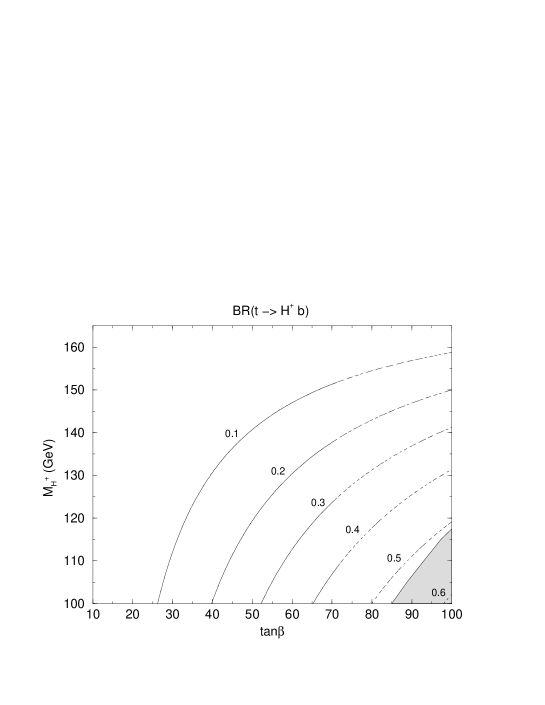
Figure 10: Curves of constant branching ratio for the $t\rightarrow b\,H^{+}$ channel. The figure shows the QCD-improved, eq. (3.1), result. The transition between the solid and dashed styles occurs when the bottom Yukawa coupling crosses the bound $h_{b}(m_{t})<1.2$. As explained in the text, this bound guarantees the perturbativity of the Yukawa up to the GUT scale. Finally, the shaded area defines the 95% C.L. exclusion boundary in the $\tan\!\beta$–$M_{H^{+}}$ plane for $m_{t}=175$ GeV and $\sigma(t\bar{t})=5.5$ pb that can be derived from the D0 frequentist analysis in ref. [5].

         

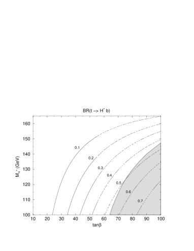
Figure 11: As fig. 10, but plotting the MSSM-improved result, eq. (3.3), for $\mu=500$ GeV (left plot) and $\mu=-500$ GeV (right plot). The rest of relevant SUSY parameters are given by $M_{\tilde{g}}=M_{2}=m_{\tilde{t}_{{1}}}=m_{\tilde{b}_{{1}}}=1$ TeV, $A_{t}=500$ GeV. In the $\mu=-500$ GeV plot, the shaded area is excluded by the D0 frequentist analysis in ref. [5].

         

Figure 12: Curves of constant branching ratio for the $H^{+}\rightarrow t\,\bar{b}$ channel. On the left, the QCD-improved values, eq. (3.1), on the right, the MSSM-improved result, eq. (3.3). The parameters chosen for these plots are $\mu=500$ GeV, $M_{\tilde{g}}=M_{2}=m_{\tilde{t}_{{1}}}=m_{\tilde{b}_{{1}}}=1$ TeV, $A_{t}=-500$ GeV.

6 Conclusions

Using an effective lagrangian description of the MSSM, we have investigated the virtual supersymmetric effects that modify the tree-level relation between the bottom Yukawa coupling and the bottom mass, which are dominant in the large $\tan\!\beta$ regime. Motivated by the fact that these effects do not vanish for large values of the SUSY masses and are potentially of ${\cal O}(1)$, we have derived the expressions for the bottom Yukawa couplings that resum all higher-order $\tan\!\beta$-enhanced quantum effects. These expressions have a natural interpretation and are easily deduced in the context of the effective lagrangian formulation. We have also shown that they can be equivalently deduced in the framework of the full MSSM.

As an interesting application of our results, we have computed the partial decay rates for the $t\rightarrow b\,H^{+}$ and $H^{+}\rightarrow t\,\bar{b}$ decay channels, relevant to supersymmetric charged Higgs searches at present and future colliders. First we have considered the QCD quantum corrections to these processes and, applying the OPE, we have performed the resummation of the leading and next-to-leading logarithms of the form $\log\,Q/m_{b}$. Concerning the supersymmetric corrections, we have compared our results with those of previous diagrammatic one-loop analyses in the literature and we have shown the numerical relevance of the resummation of the $\tan\!\beta$-enhanced effects derived in this work. Collecting the above improvements, we have finally computed the corresponding branching ratios, ${\cal BR}(t\rightarrow b\,H^{+})$ and ${\cal BR}(H^{+}\rightarrow t\,\bar{b})$. As an example, we have shown, for different sets of the MSSM parameters, the effect of the quantum corrections in determining the region of the $M_{H^{+}}$–$\tan\!\beta$ plane excluded by the D0 indirect searches for a supersymmetric charged Higgs boson in the decay of the top quark.

Appendix A The effect of $\Delta m_{b}$ at all orders

In this appendix we perform the resummation, in perturbation theory, of the leading supersymmetric effects contained in $\Delta m_{b}$ and find agreement with the effective lagrangian result of sect. 2.

When relating $\tan\!\beta$ to physical decay rates or to quark masses and Yukawa couplings one also has to address the question of the proper treatment of standard QCD corrections. This issue seems to come into play in the very beginning when one defines the renormalization scheme and scale for the bottom quark mass, which, for example, enters the off-diagonal elements of the $b$-squark mass matrix. Here we want to stress that the issues of large supersymmetric $\tan\!\beta$-enhanced corrections related to the diagram in fig. 4 and the treatment of standard QCD corrections related to gluonic corrections to the quark self-energy can be treated independently of each other. In the following we shall concentrate on the $\tan\!\beta$-enhanced SUSY-QCD corrections, induced by supersymmetric particle loop effects. After performing the resummation of these corrections to all orders in perturbation theory, one can subsequently include the standard QCD corrections, whose proper treatment is discussed in sect. 2.

The quantity $\Delta m_{b}$ is proportional to $(\alpha_{s}/\pi)(\mu\tan\!\beta/M_{SUSY})$ and of ${\cal O}(1)$ when, simultaneously, $\mu\sim M_{SUSY}$ and $\tan\!\beta$ is large. In that case one should resum its effects to all orders in PT to obtain a reliable prediction. As was shown in section 2, the first thing one should realize is that there are no higher-loop diagrams contributing to the mass renormalization (nor to the decay rate) of order $\alpha_{s}^{n}\tan^{n}\!\beta$ with $n>1$. Diagrams with extra $\mu\tan\!\beta$ insertions are suppressed by powers of $m_{b}^{2}/M_{SUSY}^{2}$. This can be easily seen in the effective lagrangian approach, where such contributions would arise from higher-dimensional operators with more Higgs boson fields, whose couplings are suppressed by extra powers of $M_{SUSY}$.

Different renormalization schemes use different values for the renormalized bottom Yukawa coupling $h_{b}$ [22]. In theories with spontaneous symmetry breaking, though, there is always a link between the value of $h_{b}$ and the physical bottom mass, $m_{b}$: the dressed bottom propagator must have a pole for on-shell external legs, or conversely the inverse propagator must vanish. At one loop this relation reads, considering only the gluino corrections

$$h_{b}v_{1}+\delta h_{b}v_{1}+h_{b}v_{1}\,\Delta m_{b}=m_{b}\,,$$ (37)

$\delta h_{b}$ being the counterterm of $h_{b}$. The l.h.s. of the previous equation is graphically depicted in fig. 13.

$$\begin{array}[]{cccc}\begin{picture}(60.0,40.0)\immediate\ignorespaces\immediate\ignorespaces\immediate\ignorespaces\immediate\ignorespaces\immediate\ignorespaces\put(0.0,0.0){\includegraphics{self1loop.1}}\ignorespaces\immediate\ignorespaces\immediate\ignorespaces\immediate\ignorespaces\immediate\ignorespaces\immediate\ignorespaces\immediate\ignorespaces \immediate\ignorespaces{}\end{picture}&\hskip 11.38092pt\begin{picture}(60.0,40.0)\immediate\ignorespaces\immediate\ignorespaces\immediate\ignorespaces\immediate\ignorespaces\immediate\ignorespaces\put(0.0,0.0){\includegraphics{self1loop.2}}\ignorespaces\immediate\ignorespaces\immediate\ignorespaces\immediate\ignorespaces\immediate\ignorespaces\immediate\ignorespaces\immediate\ignorespaces\immediate\ignorespaces\immediate\ignorespaces\immediate\ignorespaces \immediate\ignorespaces{\put(-15.0,20.0){\makebox(0.0,0.0)[l]{$+$}}}\end{picture}&\hskip 11.38092pt\begin{picture}(90.0,40.0)\immediate\ignorespaces\immediate\ignorespaces\immediate\ignorespaces\immediate\ignorespaces\immediate\ignorespaces\put(0.0,0.0){\includegraphics{self1loop.3}}\ignorespaces\immediate\ignorespaces\immediate\ignorespaces\immediate\ignorespaces\immediate\ignorespaces\immediate\ignorespaces\immediate\ignorespaces\immediate\ignorespaces\immediate\ignorespaces\immediate\ignorespaces\immediate\ignorespaces \immediate\ignorespaces{\put(-13.49945,20.0){\makebox(0.0,0.0)[l]{$+$}}\put(45.00002,14.0){\makebox(0.0,0.0)[t]{$\tilde{b}_{a}$}}\put(45.0,43.30785){\makebox(0.0,0.0)[b]{$\tilde{g}$}}}\end{picture}\end{array}$$

Figure 13: Feynman diagrams contributing to the bottom pole mass up to first order in PT. From left to right, the renormalized bottom mass, the bottom mass counterterm and the finite one-loop Feynman graph contributions are shown. The dashed line in the last diagram denotes a sbottom and the solid line a gluino. The cross represents the insertion of the bottom mass counterterm.

We are not displaying the wave function renormalization to avoid an unnecessary complication of the argument. Note that $v_{1}$ receives no one-loop QCD corrections and thus its renormalization only adds effects suppressed by $\alpha_{EW}/\alpha_{s}$, which allows us to identify $\delta h_{b}v_{1}$ with $\delta m_{b}$. Besides, in any renormalization scheme one has $m_{b}^{R}=h_{b}v_{1}$, with $m_{b}^{R}$ and $h_{b}$ denoting renormalized quantities. Therefore,

$$\left(h_{b}+\delta h_{b}\right)v_{1}=m_{b}^{R}+\delta m_{b}\,,$$ (38)

and one obtains, at first order

$$m_{b}^{R}+\delta m_{b}=m_{b}-m_{b}^{R}\Delta m_{b}.$$ (39)

The l.h.s. of eq. (39) is just the bare bottom mass, $m_{b}^{0}$.

When evaluated beyond first order, scheme differences appear in the r.h.s. of eq. (39). In the on-shell scheme, the renormalization condition being given by $m_{b}=h_{b}v_{1}=m_{b}^{R}$, one would obtain that the bare bottom mass is equal to $m_{b}\left(1-\Delta m_{b}\right)$, while in the $\overline{\mathrm{MS}}$-scheme, for which $\delta\overline{m}_{b}$ is zero as $\Delta m_{b}$ is finite, one would have $m_{b}/(1+\Delta m_{b})$. Both results are equivalent at first order in $\Delta m_{b}$, as they should.

To proceed with the resummation, we come back to the relation between the Yukawa and the pole mass. Although no $n$-loop diagrams produce $\alpha_{s}^{n}\tan^{n}\!\beta$ corrections for $n\geq 2$, there is one and only one genuine $n$-th-order diagram left (see fig. 14), which contains the insertion of a $(n-1)$-loop counterterm into a one-loop diagram. Then, all dominant terms in the large $\tan\!\beta$ limit, at all orders in PT, are contained in the equation

$$h_{b}v_{1}+\delta h_{b}v_{1}+\tilde{h}_{b}v_{1}\,\Delta m_{b}+\delta\tilde{h}_{b}v_{1}\,\Delta m_{b}=m_{b}.$$ (40)

$$\begin{array}[]{cccc}\begin{picture}(60.0,40.0)\immediate\ignorespaces\immediate\ignorespaces\immediate\ignorespaces\immediate\ignorespaces\immediate\ignorespaces\put(0.0,0.0){\includegraphics{self.1}}\ignorespaces\immediate\ignorespaces\immediate\ignorespaces\immediate\ignorespaces\immediate\ignorespaces\immediate\ignorespaces\immediate\ignorespaces \immediate\ignorespaces{}\end{picture}&\hskip 11.38092pt\begin{picture}(60.0,40.0)\immediate\ignorespaces\immediate\ignorespaces\immediate\ignorespaces\immediate\ignorespaces\immediate\ignorespaces\put(0.0,0.0){\includegraphics{self.2}}\ignorespaces\immediate\ignorespaces\immediate\ignorespaces\immediate\ignorespaces\immediate\ignorespaces\immediate\ignorespaces\immediate\ignorespaces\immediate\ignorespaces\immediate\ignorespaces\immediate\ignorespaces \immediate\ignorespaces{\put(-15.0,20.0){\makebox(0.0,0.0)[l]{$+$}}}\end{picture}&\hskip 11.38092pt\begin{picture}(90.0,40.0)\immediate\ignorespaces\immediate\ignorespaces\immediate\ignorespaces\immediate\ignorespaces\immediate\ignorespaces\put(0.0,0.0){\includegraphics{self.3}}\ignorespaces\immediate\ignorespaces\immediate\ignorespaces\immediate\ignorespaces\immediate\ignorespaces\immediate\ignorespaces\immediate\ignorespaces\immediate\ignorespaces\immediate\ignorespaces\immediate\ignorespaces\immediate\ignorespaces \immediate\ignorespaces{\put(-13.49945,20.0){\makebox(0.0,0.0)[l]{$+$}}}\end{picture}&\hskip 11.38092pt\begin{picture}(90.0,40.0)\immediate\ignorespaces\immediate\ignorespaces\immediate\ignorespaces\immediate\ignorespaces\immediate\ignorespaces\put(0.0,0.0){\includegraphics{self.4}}\ignorespaces\immediate\ignorespaces\immediate\ignorespaces\immediate\ignorespaces\immediate\ignorespaces\immediate\ignorespaces\immediate\ignorespaces\immediate\ignorespaces\immediate\ignorespaces\immediate\ignorespaces\immediate\ignorespaces\immediate\ignorespaces \immediate\ignorespaces{\put(-13.49945,20.0){\makebox(0.0,0.0)[l]{$+$}}}\end{picture}\end{array}$$

Figure 14: Full set of SUSY-QCD dominant diagrams, in the large $\tan\!\beta$ limit, contributing to the bottom pole mass at all orders in PT. The first three diagrams are those of fig. 13. In the fourth one, the cross denotes the insertion of the $\delta\tilde{h}_{b}$ counterterm, and the solid and dashed lines denote gluino and sbottom propagators respectively (see fig. 16).

Beyond tree level, the $\tilde{b}_{L}\tilde{b}_{R}H_{2}^{0}$ coupling is no longer equal to $h_{b}$, so it is denoted by $\tilde{h}_{b}$, with counterterm $\delta\tilde{h}_{b}$. This fact was not important in eq. (37) because we were just considering the first-order result.

Before proceeding, one technical point in equation (40) deserves further clarification. The last term in the l.h.s. corresponds to the true three-point diagram in fig. 14. In the large $\tan\!\beta$ limit, though, its value, $\delta\tilde{h}_{b}v_{1}\Delta m_{b}$, coincides with the two-point contribution, $\tilde{h}_{b}v_{1}\Delta m_{b}$, after replacing the renormalized coupling by the counterterm. A derivation of this result is written at the end of this appendix.

The last step in our argument is to justify the equality

$$h_{b}+\delta h_{b}=\tilde{h}_{b}+\delta\tilde{h}_{b}\,,$$ (41)

which can be regarded as the identity of the bare quark and squark Yukawa couplings, which is guaranteed by the underlying supersymmetry governing the relations between the bare lagrangian parameters in the ultraviolet. No soft SUSY-breaking dimensionful couplings can induce modifications to eq. (41), allowing for the extraction of a common $h_{b}v_{1}+\delta h_{b}v_{1}$ factor in (40). At the level of bare couplings one does not need to make reference to any particular renormalization scheme. Thus, one has

$$\left(h_{b}+\delta h_{b}\right)v_{1}=m_{b}^{R}+\delta m_{b}=\frac{m_{b}}{1+\Delta m_{b}},$$ (42)

where the r.h.s. is expressed in terms of physical quantities, $\Delta m_{b}$ being independent of $m_{b}$.

For the rest of this appendix we will derive expressions valid to all orders in PT in the large $\tan\!\beta$ limit for the $H^{+}$ and $H,h,A$ dressed couplings to $t\bar{b}$ and $b\bar{b}$ respectively, recovering the effective lagrangian results one can find in [24]. The calculation involves contributions from three-point loop diagrams with one external on-shell Higgs leg whose momentum we have neglected. In section 4, the departure from this assumption for the $H^{+}$ and $t$ decay rates has been shown to be small, as the extra contribution inducing the momentum dependence does not include any $\tan\!\beta$ enhancement factor. More complete formulae including the momentum dependence for the decay rates of the neutral Higgs bosons can be found in ref. [30].

Let us start with the simplest case, that of the charged Higgs $H^{+}$ and of the pseudoscalar $A$, for which there are no vertex loop diagrams $\tan\!\beta$-enhanced with respect to the tree-level coupling. The relevant Feynman diagrams are just the tree-level Yukawa and the counterterm. From eq. (42), the renormalized decay amplitudes are given by

$$i\left(h_{b}+\delta h_{b}\right)\sin\beta\,H^{+}\bar{t}P_{R}b = i\,\frac{m_{b}\tan\!\beta}{\left(1+\Delta m_{b}\right)v}\,H^{+}\bar{t}P_{R}b\,,$$

$$-\left(h_{b}+\delta h_{b}\right)\frac{\sin\beta}{\sqrt{2}}\,A\bar{b}\gamma_{5}b = -\frac{m_{b}\tan\!\beta}{\sqrt{2}\left(1+\Delta m_{b}\right)v}\,A\bar{b}\gamma_{5}b\,.$$ (43)

Therefore, in this case, the result of the resummation is to effectively modify the tree-level Yukawa coupling by the universal $1/(1+\Delta m_{b})$ factor.

The case of the CP-even neutral Higgs bosons is a little bit more involved. Depending on the relation between $\beta$ and the mixing angle, $\alpha$, the one-loop correction to the vertex diagrams can be importantly enhanced. The full set of potentially relevant graphs is shown in fig. 15.

$$\begin{array}[c]{cccc}\begin{picture}(80.0,70.0)\immediate\ignorespaces\immediate\ignorespaces\immediate\ignorespaces\immediate\ignorespaces\immediate\ignorespaces\put(0.0,0.0){\includegraphics{yukawa.1}}\ignorespaces\immediate\ignorespaces\immediate\ignorespaces\immediate\ignorespaces\immediate\ignorespaces\immediate\ignorespaces\immediate\ignorespaces\immediate\ignorespaces \immediate\ignorespaces{}\end{picture}&\begin{picture}(80.0,70.0)\immediate\ignorespaces\immediate\ignorespaces\immediate\ignorespaces\immediate\ignorespaces\immediate\ignorespaces\put(0.0,0.0){\includegraphics{yukawa.2}}\ignorespaces\immediate\ignorespaces\immediate\ignorespaces\immediate\ignorespaces\immediate\ignorespaces\immediate\ignorespaces\immediate\ignorespaces\immediate\ignorespaces\immediate\ignorespaces\immediate\ignorespaces\immediate\ignorespaces \immediate\ignorespaces{\put(-15.99976,35.0){\makebox(0.0,0.0)[l]{$+$}}}\end{picture}&\begin{picture}(90.0,70.0)\immediate\ignorespaces\immediate\ignorespaces\immediate\ignorespaces\immediate\ignorespaces\immediate\ignorespaces\put(0.0,0.0){\includegraphics{yukawa.3}}\ignorespaces\immediate\ignorespaces\immediate\ignorespaces\immediate\ignorespaces\immediate\ignorespaces\immediate\ignorespaces\immediate\ignorespaces\immediate\ignorespaces\immediate\ignorespaces\immediate\ignorespaces\immediate\ignorespaces\immediate\ignorespaces\immediate\ignorespaces\immediate\ignorespaces \immediate\ignorespaces{\put(-17.99973,35.0){\makebox(0.0,0.0)[l]{$+$}}\put(45.48334,21.53755){\makebox(0.0,0.0)[rt]{$\tilde{b}_{a}$}}\put(72.27238,35.0){\makebox(0.0,0.0)[l]{$\tilde{g}$}}\put(45.48334,48.4624){\makebox(0.0,0.0)[rb]{$\tilde{b}_{b}$}}}\end{picture}&\,\,\,\,\begin{picture}(90.0,70.0)\immediate\ignorespaces\immediate\ignorespaces\immediate\ignorespaces\immediate\ignorespaces\immediate\ignorespaces\put(0.0,0.0){\includegraphics{yukawa.4}}\ignorespaces\immediate\ignorespaces\immediate\ignorespaces\immediate\ignorespaces\immediate\ignorespaces\immediate\ignorespaces\immediate\ignorespaces\immediate\ignorespaces\immediate\ignorespaces\immediate\ignorespaces\immediate\ignorespaces\immediate\ignorespaces\immediate\ignorespaces\immediate\ignorespaces\immediate\ignorespaces \immediate\ignorespaces{\put(-17.99973,35.0){\makebox(0.0,0.0)[l]{$+$}}\put(45.48334,21.53755){\makebox(0.0,0.0)[rt]{$\tilde{b}_{a}$}}\put(72.27238,35.0){\makebox(0.0,0.0)[l]{$\tilde{g}$}}\put(45.48334,48.4624){\makebox(0.0,0.0)[rb]{$\tilde{b}_{b}$}}}\end{picture}\end{array}$$

Figure 15: Vertex diagrams contributing to the renormalization of the Higgs-fermion Yukawa interaction. From left to right, the renormalized Yukawa coupling, the Yukawa counterterm, the one-loop contribution and the higher-order diagram containing the insertion of the $\delta\tilde{h}_{b}$ counterterm. The solid and dashed lines inside the loops denote gluino and sbottom propagators respectively. The cross in the fourth diagram denotes the $\delta\tilde{h}_{b}$ counterterm.

One obtains, for the $H\bar{b}b$ renormalized amplitude

$$-i\left(h_{b}+\delta h_{b}\right)\frac{\cos\alpha}{\sqrt{2}}\,H\bar{b}b-i\left(\tilde{h}_{b}+\delta\tilde{h}_{b}\right)\frac{\sin\alpha}{\sqrt{2}}\frac{\Delta m_{b}}{\tan\!\beta}\,H\bar{b}b =$$

$$-i\,\frac{m_{b}\cos\alpha}{\sqrt{2}\left(1+\Delta m_{b}\right)v_{1}}\left(1+\Delta m_{b}\frac{\tan\alpha}{\tan\!\beta}\right)\,H\bar{b}b\,.$$ (44)

Again, the resummation amounts to the inclusion of the universal $1/(1+\Delta m_{b})$ factor. However, there is an additional $\Delta m_{b}$ term inside the parenthesis, which constitutes the non $\tan\!\beta$-suppressed contribution coming from the SUSY-QCD vertex diagrams. Similarly, for the $h\bar{b}b$ one has

$$i\left(h_{b}+\delta h_{b}\right)\frac{\sin\alpha}{\sqrt{2}}\,h\bar{b}b-i\left(\tilde{h}_{b}+\delta\tilde{h}_{b}\right)\frac{\cos\alpha}{\sqrt{2}}\frac{\Delta m_{b}}{\tan\!\beta}\,h\bar{b}b =$$

$$i\,\frac{m_{b}\sin\alpha}{\sqrt{2}\left(1+\Delta m_{b}\right)v_{1}}\left(1-\frac{\Delta m_{b}}{\tan\alpha\tan\!\beta}\right)\,h\bar{b}b\,.$$ (45)

It can easily be checked that for large $M_{H^{+}}$ values, the limit that corresponds to the effective decoupling of one of the Higgs doublets, one recovers the SM $h\bar{b}b$ coupling

$$-i\,\frac{m_{b}}{\sqrt{2}v}\,h\bar{b}b\,,$$

whereas the $H\bar{b}b$ coupling, $H$ being heavy, still “feels” the decoupled sector

$$-i\,\frac{m_{b}\tan\!\beta}{\sqrt{2}\left(1+\Delta m_{b}\right)v}\,H\bar{b}b\,.$$

Figure 16: The fourth self-energy diagram in fig. 14, shown in greater detail. A gluino propagator is denoted by the solid line inside the loop. The dashed lines denote sbottom propagators and the cross the insertion of a $\delta\tilde{h}_{b}$ counterterm.

Two-point–three-point diagram identity

Let us evaluate the amplitude associated to the three-point Feynman diagram of fig. 16. Neglecting the external momentum, it can be written

$$-\left(8\pi\alpha_{s}\right)\,C_{F}\,\frac{\delta\tilde{h}_{b}v_{1}}{\sqrt{2}}\,M_{\tilde{g}}\,\mu\tan\!\beta\int\frac{d^{n}k}{(2\pi)^{n}}\,\frac{\left(Z_{i1}Z_{j2}^{*}+Z_{i2}Z_{j1}^{*}\right)\,Z_{j2}Z_{i1}^{*}}{(k^{2}-M_{\tilde{g}})(k^{2}-m_{\tilde{b}_{{i}}}^{{2}})(k^{2}-m_{\tilde{b}_{{j}}}^{{2}})}\,\bar{b}P_{L}b\,,$$ (46)

where $C_{F}=4/3$ is a colour factor and the two-dimensional rotation matrices $Z$ transform the weak eigenstate sbottom basis into the mass eigenstate basis. Expressed in terms of the mixing angle $\theta_{\tilde{b}}$, the components of $Z$ read: $Z_{11}=Z_{22}=\cos\!\theta_{\tilde{b}}$, $Z_{12}=-Z_{21}=\sin\!\theta_{\tilde{b}}$. The term between parentheses in the numerator of (46) and the combination $\delta\tilde{h}_{b}v_{2}=\delta\tilde{h}_{b}v_{1}\tan\!\beta$ come from the counterterm to the $\tan\!\beta$-dominant interaction $H_{2}^{0}\tilde{b}_{R}^{*}\tilde{b}_{L}$, after the Higgs field develops its vacuum expectation value $v_{2}$.

Splitting the implicit $i,j$ sum into the $i=j$ part and the rest of the terms we obtain

$$\frac{\kappa}{2}\,\sin^{2}\!2\theta_{\tilde{b}}\int\frac{d^{n}k}{(2\pi)^{n}}\,\frac{1}{k^{2}-M_{\tilde{g}}^{2}}\left(\frac{1}{(k^{2}-m_{\tilde{b}_{{1}}}^{{2}})^{2}}+\frac{1}{(k^{2}-m_{\tilde{b}_{{2}}}^{{2}})^{2}}\right)\,\bar{b}P_{L}b$$ (47)

$$+ \kappa\cos^{2}\!2\theta_{\tilde{b}}\int\frac{d^{n}k}{(2\pi)^{n}}\,\frac{1}{(k^{2}-M_{\tilde{g}}^{2})(k^{2}-m_{\tilde{b}_{{1}}}^{{2}})(k^{2}-m_{\tilde{b}_{{2}}}^{{2}})}\,\bar{b}P_{L}b\,,$$

the constant $\kappa$ being a short-hand for the constant prefactor of the integral in (46).

The second term in (47) is of the same form as $\Delta m_{b}$. Adding and removing this term times $\tan^{2}\!2\theta_{\tilde{b}}$ and rearranging terms one arrives at

$$\kappa\int\frac{d^{n}k}{(2\pi)^{n}}\,\frac{1}{(k^{2}-M_{\tilde{g}}^{2})(k^{2}-m_{\tilde{b}_{{1}}}^{{2}})(k^{2}-m_{\tilde{b}_{{2}}}^{{2}})}\,\bar{b}P_{L}b$$ (48)

$$+ \frac{\kappa}{2}\,\sin^{2}\!2\theta_{\tilde{b}}\int\frac{d^{n}k}{(2\pi)^{n}}\frac{1}{k^{2}-M_{\tilde{g}}^{2}}\,\frac{(m_{\tilde{b}_{{2}}}^{{2}}-m_{\tilde{b}_{{1}}}^{{2}})^{2}}{(k^{2}-m_{\tilde{b}_{{1}}}^{{2}})^{2}(k^{2}-m_{\tilde{b}_{{2}}}^{{2}})^{2}}\,\bar{b}P_{L}b\,.$$

Now one can make use of the tree-level relation

$$\sin\!2\theta_{\tilde{b}} = \frac{2m_{b}\left(A_{b}-\mu\tan\!\beta\right)}{m_{\tilde{b}_{{1}}}^{{2}}-m_{\tilde{b}_{{2}}}^{{2}}}$$ (49)

to write ($A_{b}$ is dropped since it is not $\tan\!\beta$-enhanced)

$$\kappa\int\frac{d^{n}k}{(2\pi)^{n}}\,\frac{1}{(k^{2}-M_{\tilde{g}}^{2})(k^{2}-m_{\tilde{b}_{{1}}}^{{2}})(k^{2}-m_{\tilde{b}_{{2}}}^{{2}})}\,\bar{b}P_{L}b$$ (50)

$$+ 2\kappa\,m_{b}^{2}\left(\mu\tan\!\beta\right)^{2}\int\frac{d^{n}k}{(2\pi)^{n}}\frac{1}{(k^{2}-M_{\tilde{g}}^{2})(k^{2}-m_{\tilde{b}_{{1}}}^{{2}})^{2}(k^{2}-m_{\tilde{b}_{{2}}}^{{2}})^{2}}\,\bar{b}P_{L}b\,.$$

The second integral in (50) has two extra propagators and thus in the limit of heavy SUSY masses it is of ${\cal O}(1/M_{SUSY}^{6})$, whereas the first one is of ${\cal O}(1/M_{SUSY}^{2})$. One can conclude that the two- and three-point loop diagrams in fig. 14 are just related by $\delta\tilde{h}_{b}/\tilde{h}_{b}$, apart from contributions that are suppressed by powers of either $\tan\!\beta$ or $m_{b}^{2}\tan^{2}\!\beta/M_{SUSY}^{2}$. The amplitude for the diagram in fig. 16 reduces to

$$i\,\delta\tilde{h}_{b}v_{1}\,\Delta m_{b}\left[1+\frac{\mu^{2}}{M_{SUSY}^{2}}\,\times\,{\cal O}\left(\frac{m_{b}^{2}\tan^{2}\!\beta}{M_{SUSY}^{2}}\right)\,+\,{\cal O}\left(\frac{1}{\tan\!\beta}\right)\right]\,\bar{b}P_{L}b\,.$$ (51)

Appendix B Large logarithms in decay rates

Our effective lagrangian ${\cal L}$ in eq. (20) contains the large logarithms associated with the running of the Yukawa couplings to all orders in perturbation theory. In general this procedure does not sum all the large logarithms that appear in a specific cross section or decay rate. In this appendix we show that for $\Gamma(t\rightarrow b\,H^{+})$ and $\Gamma(H^{+}\rightarrow t\,\bar{b})$ such additional, process-specific logarithms do not occur except in highly power-suppressed, numerically negligible terms.

Let us first consider the decay $H^{+}\rightarrow t\,\bar{b}$: the optical theorem relates the decay rate to the imaginary part of the $H^{+}$ self-energy:

$$\Gamma(H^{+}\rightarrow t\,\bar{b}) = \frac{1}{M_{H^{+}}}\left.\mbox{Im\hskip 2.84526pt}i\int d^{4}x\,e^{-iq\cdot x}\langle\,H^{+}\,|{\cal T}J^{\dagger}(x)J(0)|\,H^{+}\,\rangle\right|_{q^{2}=M_{H^{+}}^{2}}.$$ (52)

Here

$$J(x) = \frac{g}{\sqrt{2}M_{W}}\frac{\overline{m}_{b}(Q)}{1+\Delta m_{b}}\,V_{tb}\,\tan\!\beta\,H^{+}\,\overline{t}_{L}b_{R}(x,Q)$$

is the scalar current stemming from the Yukawa interaction in eq. (20). All currents and couplings in this appendix are considered to be renormalized using a mass-independent renormalization scheme such us the $\overline{\rm MS}$ scheme [28]. For the moment we also assume this for the quark masses and discuss the use of the pole mass definition, which is commonly used for the top mass, later. The decay rate involves highly separated mass scales $m_{b}\ll M_{H^{+}},m_{t}$. First we assume that $M_{H^{+}}$ and $m_{t}$ are of similar size so that $\log M_{H^{+}}/m_{t}$ is not dangerously large. We return to the case $m_{b}\ll m_{t}\ll M_{H^{+}}$ later. To prepare the resummation of the large logarithm $\log m_{b}/M_{H^{+}}$, we first perform an operator product expansion of the bilocal forward scattering operator in eq. (52):

$$\!\!i\!\int\!\!d^{4}x\,e^{-iq\cdot x}\langle\,H^{+}\,|{\cal T}J^{\dagger}(x)J(0)|\,H^{+}\,\rangle = \sum_{n}C_{n}\left(q^{2},m_{t},Q\right)\langle\,H^{+}\,|{\cal O}_{n}|\,H^{+}\,\rangle\left(m_{b},Q\right).$$ (53)

Here all dependence on the heavy mass scales $m_{t}$ and $q^{2}=M_{H^{+}}^{2}$ is contained in the Wilson coefficient $C_{n}$, while the dependence on the light scale $m_{b}$ resides in the matrix element of the local operator ${\cal O}_{n}$. Both depend on the renormalization scale $Q$ at which the OPE is carried out (so that $Q$ is sometimes called factorization scale). The OPE provides an expansion of $\Gamma(H^{+}\rightarrow t\,\bar{b})$ in terms of $(m_{b}/M_{H^{+}})^{2}$. Increasing powers of $m_{b}/M_{H^{+}}$ correspond to increasing twists of the local operator ${\cal O}_{n}$. Here the twist is defined as the dimension of the operator ${\cal O}_{n}$ minus the number of derivatives acting on the Higgs fields in ${\cal O}_{n}$.

The OPE in eq. (53) is depicted in fig. 17 where also the leading twist operator ${\cal O}_{1}=\overline{m}_{b}^{2}(Q)H^{+}H^{-}$ is shown. At leading twist the OPE, depicted in fig. 17, is trivial: the matrix element $\langle\,H^{+}\,|{\cal O}_{1}|\,H^{+}\,\rangle$ simply equals $\overline{m}_{b}^{2}(Q)$ and the Wilson coefficient $C_{1}$ can be read off from eq. (3.3). In the leading order (LO) of QCD it reads

Figure 17: The OPE in (53) to leading order in $m_{b}/M_{H^{+}}$ and $\alpha_{s}$. The self-energy diagram on the left represents the left-hand side of eq. (53). The right diagram depicts $\langle\,H^{+}\,|{\cal O}_{1}|\,H^{+}\,\rangle$.

$$\mbox{Im\hskip 2.84526pt}C_{1} = \frac{g^{2}N_{c}}{32\pi M_{W}^{2}}\,M_{H^{+}}^{2}\,\left(1-r_{t}\right)^{2}\frac{1}{\left(1+\Delta m_{b}\right)^{2}}\,\tan^{2}\!\beta.$$ (54)

The QCD radiative corrections in $\Gamma$ contain powers of the large logarithm $\alpha_{s}\log m_{b}/M_{H^{+}}$. The OPE in eq. (53) splits this logarithm into $\alpha_{s}\log Q/M_{H^{+}}+\alpha_{s}\log m_{b}/Q$: the former term resides in the coefficient function $C_{1}$ while the latter is contained in the matrix element $\langle\,H^{+}\,|{\cal O}_{1}|\,H^{+}\,\rangle$. If we choose $Q={\cal O}(m_{t},M_{H^{+}})$, then the logarithms in the Wilson coefficient are small and perturbative, but $\log m_{b}/Q$ in the matrix element is big and needs to be resummed to all orders. One could likewise choose $Q\simeq m_{b}$ and resum the large logarithm in the Wilson coefficient, but the former way is much easier here. In order to sum $\log m_{b}/Q$ we have to solve the renormalization group (RG) equation for ${\cal O}_{1}$. Since the Higgs fields in ${\cal O}_{1}$ have no QCD interaction, the solution of the RG equation simply amounts to the use of the well-known result for the running quark mass $m_{b}(Q)$ (see eq. (17)) at the scale $Q={\cal O}(m_{t},M_{H^{+}})$ in ${\cal O}_{1}$. In the next-to-leading (NLO) order one has to include the ${\cal O}(\alpha_{s})$ corrections to $\Gamma$ in eq. (3.3). First there are no explicit one-loop corrections to $\langle\,H^{+}\,|{\cal O}_{1}|\,H^{+}\,\rangle$, so that in the NLO we obtain $\mbox{Im\hskip 2.84526pt}C_{1}(Q)$ by simply multiplying the result in eq. (54) with the curly bracket in (3.3). Secondly in the NLO we have to use the two-loop formula for $\overline{m}_{b}(Q)$ in the matrix element. Since one is equally entitled to use $Q=M_{H^{+}}$ (as chosen in (3.3)) or $Q=m_{t}$ or any other scale of order $m_{t},M_{H^{+}}$, there is a residual scale uncertainty. This feature is familiar from all other RG-improved observables. To the calculated order $\alpha_{s}$ this uncertainty cancels, because there is an explicit term $\alpha_{s}\log Q/M_{H^{+}}$ in the one-loop correction, so that the scale uncertainty is always of the order of the next uncalculated term. In our case this is ${\cal O}(\alpha_{s}^{2})$ and numerically tiny. In conclusion, our OPE analysis shows that at leading order in $m_{b}/M_{H^{+}}$ all large logarithms in $\Gamma(H^{+}\rightarrow t\,\bar{b})$ can indeed be absorbed into the running quark mass in our effective lagrangian in eq. (20). Some clarifying points are in order:

• The summation of large logarithms in the NLO does not require the calculation of the two-loop diagrams obtained by dressing the diagram in fig. 17 with an extra gluon, as performed in [31]. This calculation only gives redundant information, already contained in the known two-loop formula for the running quark mass.

• At the next-to-leading order the result depends on the chosen renormalization scheme. Changing the scheme modifies the constant term 17/3 in eq. (3.3). After inserting the NLO (two-loop) solution (17) for the running mass, this scheme dependence cancels between this term and $J^{(f)}$ in eq. (18). In the literature, sometimes, the one-loop result for $\Gamma$ is incorrectly combined with the one-loop running bottom mass resulting in a scheme-dependent expression.
  No running top-quark mass is needed for the case $m_{t}\simeq M_{H^{+}}$, and one can adopt the pole mass definition for $m_{t}$ as we did.

• The OPE also shows that the correct scale to be used in the running $\alpha_{s}$ in eq. (3.3) is the high scale $Q={\cal O}(m_{t},M_{H^{+}})$ and not the low scale $m_{b}$.

• The absorption of the large logarithms into the running mass does not work for terms that are suppressed by higher powers $(m_{b}/M_{H^{+}})^{n}$ with respect to the leading contribution considered by us. Higher-twist operators contain explicit $b$-quark fields. At twist-8 there are operators of the form $m_{b}^{3}H^{+}H^{-}\overline{b}\Delta b$, where $\Delta$ is some Dirac structure. Solving the RG equation for these operators yields extra evolution factors in addition to the running mass. These effects occur in corrections of order $m_{b}^{4}/M_{H^{+}}^{4}$ and are certainly only of academic interest.

Next consider $\Gamma(H^{+}\rightarrow t\,\bar{b})$ for the case $m_{b}\ll m_{t}\ll M_{H^{+}}$: in this limit, another large logarithm, $\log m_{t}/M_{H^{+}}$, appears. Now we have to perform the OPE in two steps. In the first step we again match the forward scattering operator to local operators as in eq. (53) at a scale $Q_{1}={\cal O}(M_{H^{+}})$, but we treat the top quark as light, so that the dependence on $m_{t}$ now resides in the matrix element $\langle\,H^{+}\,|{\cal O}_{1}|\,H^{+}\,\rangle$ rather than in the Wilson coefficient. For simplicity we specify $Q_{1}=M_{H^{+}}$. The leading power $r_{t}^{0}$ is again represented by the twist-4 operator ${\cal O}_{1}$, yet the corresponding Wilson coefficient lacks the factor of $(1-r_{t})^{2}$ compared to eq. (54). The terms of order $r_{t}^{1}$ are represented by ${\cal O}_{2}=\overline{m}_{t}^{2}{\cal O}_{1}$ with $C_{2}=-2\,C_{1}/M_{H^{+}}^{2}$. At twist-8 different operators of the form $m_{t}^{3}H^{+}H^{-}\overline{t}\Delta t$ with non-trivial anomalous dimensions occur as discussed in point 4 above. In the second step one applies an OPE at the scale $Q_{2}={\cal O}(m_{t})$. At this step the dependence on $m_{t}$ migrates from the matrix elements into the Wilson coefficients, which at order $r_{t}^{1}$ amounts to a trivial rescaling of the coefficients and operators by $m_{t}$ or $1/m_{t}$. To order $r_{t}^{0}$ and $r_{t}^{1}$ the only effect of the OPE is to replace the top mass in the expression for $\Gamma(H^{+}\rightarrow t\,\bar{b})$ in eq. (3.3) by a running top mass $\overline{m}_{t}(M_{H^{+}})$, and to omit the explicit term proportional to $r_{t}\log r_{t}$ in the ${\cal O}(\alpha_{s})$ correction. Since we have adopted the on-shell definition for the top mass, one must either use a running mass definition based on the pole mass (i.e. with $\overline{m}_{t}(m_{t})=m_{t}^{pole}$) or transform the result in eq. (3.3) to the $\overline{\rm MS}$ scheme with the appropriate change in the ${\cal O}(\alpha_{s})$ correction. It is a nice check to expand the running mass to first order in $\alpha_{s}$:

$$\overline{r}_{t}\left(M_{H^{+}}\right) = \frac{\overline{m}_{t}^{2}(M_{H^{+}})}{M_{H^{+}}^{2}}\;=\;r_{t}\,\left(1+2\,\frac{\alpha_{s}}{\pi}\log r_{t}\right)+{\cal O}\left(\alpha_{s}^{2}\right)\qquad\qquad\mbox{with }r_{t}=\overline{r}_{t}\left(m_{t}\right)$$

and to verify that the overall factor $(1-\overline{r}_{t}(M_{H^{+}}))^{2}$ indeed reproduces the $r_{t}\log r_{t}$ term in eq. (3.3). The terms of order $r_{t}^{2}\log r_{t}$ are not correctly reproduced by the running top mass as anticipated by the occurrence of non-trivial twist-8 operators. The important result of our consideration of the case $m_{b}\ll m_{t}\ll M_{H^{+}}$ is the absence of terms of the form $r_{t}^{0}\log r_{t}$ to all orders in $\alpha_{s}$. In this case the additional large logarithm $\log r_{t}$ is always suppressed by powers of $r_{t}$ and therefore these terms are negligible for $r_{t}\ll 1$ and need not be resummed.

For the decay $t\rightarrow b\,H^{+}$ the above discussion can be repeated with the appropriate changes in the OPE: the leading-twist operator is now ${\cal O}_{1}(Q)=\overline{m}_{b}^{2}(Q)\,\overline{t}t(Q)$ and the external state in eq. (53) is a top quark instead of a charged Higgs boson. We have $m_{b}\ll m_{t},M_{H^{+}}$ and the factorization scale $Q$ is again of order $m_{t},M_{H^{+}}$. While ${\cal O}_{1}$ now involves strongly interacting fields, its matrix element $\langle\,t\,|{\cal O}_{1}|\,t\,\rangle(Q)$ still does not contain large logarithms $\log m_{b}/Q$ other than those contained in the running mass $\overline{m}_{b}(Q)$. Hence the proof above for $\Gamma(H^{+}\rightarrow t\,\bar{b})$ applies likewise for $\Gamma(t\rightarrow b\,H^{+})$.

After exchanging $V_{tb}\overline{t}_{L}b_{R}$ for $V_{cb}\overline{c}_{L}b_{R}$ in eq. (20), we can likewise apply our effective lagrangian ${\cal L}$ to semileptonic $B$-meson decays corresponding to $b\rightarrow c\,\ell\,\overline{\nu}_{\ell}$ by using the appropriate scale $Q\simeq m_{b}$ in ${\cal L}$. The QCD radiative corrections involve no large logarithm, because the gluons couple only to the $b$ and $c$ quarks. Hence the effective four-fermion operator $\overline{c}_{L}b_{R}\,\overline{\ell}_{R}\nu_{L}$ obtained after integrating out the heavy $H^{+}$ renormalizes in the same way as the quark current $\overline{c}_{L}b_{R}$ in ${\cal L}$. The corresponding loop integrals do not depend on $M_{H^{+}}$ at all and this feature is correctly reproduced by using $\overline{m}_{b}(m_{b})$ in ${\cal L}$. The situation is different in physical processes in which the charged Higgs connects two quark lines, as for example in the loop-induced decay $b\rightarrow s\,\gamma$. Here effective four-quark operators, which involve a non-trivial renormalization group evolution, occur. The large-$\tan\!\beta$ supersymmetric QCD corrections associated with $\Delta m_{b}$ and the $H^{+}\overline{t}_{L}b_{R}$ Yukawa coupling, however, are still correctly reproduced by applying ${\cal L}$ to $b\rightarrow s\,\gamma$ or other loop-induced rare $b$-decays. Yet it must be clear that these corrections are part of the mixed electroweak-QCD two-loop contributions and that there are already supersymmetric electroweak contributions at the one-loop level, which are process-specific and of course not contained in ${\cal L}$.

References

- [1] S. Dimopoulos and H. Georgi, Nucl. Phys. B193 (1981) 150; N. Sakai, Z. Phys. C11 (1981) 153; K. Harada and N. Sakai, Prog. Theor. Phys. 67 (1982) 1877; L. Girardello and M.T. Grisaru, Nucl. Phys. B194 (1982) 65.
- [2] H.P. Nilles, Phys. Rep. 110 (1984) 1; H.E. Haber and G.L. Kane, Phys. Rep. 117 (1985) 75; A.B. Lahanas and D.V. Nanopoulos, Phys. Rep. 145 (1987) 1.
- [3] J.F. Gunion, H.E. Haber, G.L. Kane and S. Dawson, “The Higgs Hunter’s Guide,” Addison-Wesley, Menlo-Park, 1990.
- [4] Talk given by A. Blondel to the LEP Experiments Committee for the ALEPH collaboration, CERN, November 1999; P. Abreu et al. [DELPHI Collaboration], Phys. Lett. B460 (1999) 484.
- [5] Talk given by D. Chakraborty at the SUSY 99 conference, Fermilab, June 1999; B. Abbott et al. [D0 Collaboration], Phys. Rev. Lett. 82 (1999) 4975.
- [6] B. Bevensee [CDF Collaboration], “Top to charged Higgs decays and top properties at the Tevatron,” To be published in the proceedings of 33rd Rencontres de Moriond: QCD and High Energy Hadronic Interactions, Les Arcs, France, 21-28 Mar 1998; F. Abe et al. [CDF Collaboration], Phys. Rev. Lett. 79 (1997) 357.
- [7] F.M. Borzumati and A. Djouadi, hep-ph/9806301.
- [8] N.G. Deshpande, X. Tata and D.A. Dicus, Phys. Rev. D29 (1984) 1527; E. Eichten, I. Hinchliffe, K. Lane and C. Quigg, Rev. Mod. Phys. 56 (1984) 579; S.S. Willenbrock, Phys. Rev. D35 (1987) 173.
- [9] Z. Kunszt and F. Zwirner, Nucl. Phys. B385 (1992) 3.
- [10] J.F. Gunion and J. Kelly, Phys. Rev. D56 (1997) 1730; S. Moretti and K. Odagiri, Phys. Rev. D55 (1997) 5627; A. Krause, T. Plehn, M. Spira and P.M. Zerwas, Nucl. Phys. B519 (1998) 85; S. Moretti and K. Odagiri, Eur. Phys. J. C1 (1998) 633 and Phys. Rev. D57 (1998) 5773; A.A. Barrientos Bendezu and B.A. Kniehl, Phys. Rev. D59 (1999) 015009; S. Moretti and K. Odagiri, Phys. Rev. D59 (1999) 055008; C.S. Huang and S. Zhu, Phys. Rev. D60 (1999) 075012; F. Borzumati, J. Kneur and N. Polonsky, Phys. Rev. D60 (1999) 115011; L.G. Jin, C.S. Li, R.J. Oakes and S.H. Zhu, hep-ph/9907482; A.A. Barrientos Bendezu and B.A. Kniehl, hep-ph/9908385; O. Brein and W. Hollik, hep-ph/9908529; J.A. Coarasa, J. Guasch and J. Sola, hep-ph/9909397.
- [11] See A. Blondel in [4]; Talk given by Pat Ward to the LEP Experiments Committee for the DELPHI collaboration, CERN, November 1999.
- [12] B. Ananthanarayan, G. Lazarides and Q. Shafi, Phys. Rev. D44 (1991) 1613; T. Banks, Nucl. Phys. B303 (1988) 172; M. Olechowski and S. Pokorski, Phys. Lett. B214 (1988) 393; S. Dimopoulos, L.J. Hall and S. Raby, Phys. Rev. Lett. 68 (1992) 1984 and Phys. Rev. D45 (1992) 4192; G.W. Anderson, S. Raby, S. Dimopoulos and L.J. Hall, Phys. Rev. D47 (1993) 3702.
- [13] M. Carena, M. Olechowski, S. Pokorski and C.E.M. Wagner, Nucl. Phys. B426 (1994) 269; L.J. Hall, R. Rattazzi and U. Sarid, Phys. Rev. D50 (1994) 7048.
- [14] R.A. Jimenez and J. Sola, Phys. Lett. B389 (1996) 53; A. Bartl, H. Eberl, K. Hidaka, T. Kon, W. Majerotto and Y. Yamada, Phys. Lett. B378 (1996) 167.
- [15] J.A. Coarasa, D. Garcia, J. Guasch, R.A. Jimenez and J. Sola, Phys. Lett. B425 (1998) 329.
- [16] J. Guasch, R.A. Jimenez and J. Sola, Phys. Lett. B360 (1995) 47.
- [17] J.A. Coarasa, D. Garcia, J. Guasch, R.A. Jimenez and J. Sola, Eur. Phys. J. C2 (1998) 373.
- [18] A. Mendez and A. Pomarol, Phys. Lett. B252 (1990) 461; C. Li and R.J. Oakes, Phys. Rev. D43 (1991) 855.
- [19] A. Djouadi and P. Gambino, Phys. Rev. D51 (1995) 218.
- [20] C.S. Li and T.C. Yuan, Phys. Rev. D42 (1990) 3088; M. Drees and D.P. Roy, Phys. Lett. B269 (1991) 155; C. Li, Y. Wei and J. Yang, Phys. Lett. B285 (1992) 137.
- [21] A. Czarnecki and S. Davidson, Phys. Rev. D48 (1993) 4183.
- [22] E. Braaten and J.P. Leveille, Phys. Rev. D22 (1980) 715; M. Drees and K. Hikasa, Phys. Lett. B240 (1990) 455.
- [23] R. Harlander and M. Steinhauser, Phys. Rev. D56 (1997) 3980.
- [24] M. Carena, S. Mrenna and C.E.M. Wagner, Phys. Rev. D60 (1999) 075010, see also hep-ph/9907422.
- [25] D.M. Pierce, J.A. Bagger, K. Matchev and R. Zhang, Nucl. Phys. B491 (1997) 3.
- [26] T. Kinoshita, J. Math. Phys. 3 (1962) 650; T.D. Lee and M. Nauenberg, Phys. Rev. 133 (1964) B1549; G. Sterman, Phys. Rev. D14 (1976) 2123.
- [27] S.L. Adler, J.C. Collins and A. Duncan, Phys. Rev. D15 (1977) 1712; B. Kniehl and M. Spira, Z. Phys. C69 (1995) 77; W. Kilian, Z. Phys. C69 (1995) 89.
- [28] W.A. Bardeen, A.J. Buras, D.W. Duke and T. Muta, Phys. Rev. D18 (1978) 3998.
- [29] M. Beneke and A. Signer, hep-ph/9906475; A.H. Hoang, hep-ph/9905550.
- [30] F. Borzumati, G.R. Farrar, N. Polonsky and S. Thomas, Nucl. Phys. B555 (1999) 53.
- [31] A. Czarnecki and A. I. Davydychev, Phys. Lett. B325 (1994) 435.