Abstract

We improve the calculation of the supersymmetric ${\cal O}(\alpha_{s})$ QCD corrections to the decays of Higgs bosons into quarks and squarks in the Minimal Supersymmetric Standard Model. In the on–shell renormalization scheme these corrections can be very large, which makes the perturbative expansion unreliable. This is especially serious for decays into bottom quarks and squarks for large $\tan\beta$. Their corrected widths can even become negative. We show that this problem can be solved by a careful choice of the tree–level Higgs boson couplings to quarks and squarks, in terms of the QCD and SUSY QCD running quark masses, running trilinear couplings $A_{q}$, and on–shell left–right mixing angles of squarks. We also present numerical results for the corrected partial decay widths for the large $\tan\beta$ case.

1 Introduction

The Minimal Supersymmetric Standard Model (MSSM) [1] is a very promising extension of the Standard Model. This model has five physical Higgs scalars, $h^{0}$, $H^{0}$, $A^{0}$, and $H^{\pm}$. Studying their properties is very important for probing the nature of the breaking of the electroweak symmetry and supersymmetry.

The Higgs scalars have large couplings to quarks and scalar quarks (squarks) of the third generation [2]. Therefore, in typical cases the decays to top and bottom quarks have large branching ratios and are often the main modes, see e. g. [3]. Decays to top and bottom squarks can be also dominant [4, 5] if they are kinematically allowed and the left–right mixing parameters of the squarks are large. Studying these decays is therefore very important for the discovery and the detailed study of the Higgs bosons in the MSSM.

The decays of Higgs bosons into quarks and squarks receive large radiative corrections by QCD interactions. In the MSSM, one–loop SUSY QCD corrections to the decay widths have been given analytically, both for quark modes [6, 7, 8, 9] and squark modes [10, 11]. However, when the lowest order widths are given in terms of the on–shell parameters for quarks and squarks, the ${\cal O}(\alpha_{s})$ correction terms are often comparable to or even larger than the lowest order ones, especially for decays into bottom quark and squark. Such large corrections make the perturbation calculation of the decay widths quite unreliable. When the correction term is negative, the corrected width can even become negative, which clearly makes no sense. This “negative width” problem has also been observed in other processes of squarks [12].

The couplings of Higgs bosons to quarks and squarks depend on the quark masses $m_{q}$. For the decays into quarks, it is well known [13, 14] that the large part of the gluon loop correction can be absorbed by giving the tree–level Higgs–quark couplings in terms of the QCD running quark masses $m_{q}(Q)_{\rm SM}$, where $Q$ is at the scale of the parent Higgs boson mass. The convergence of the perturbation series is greatly improved by this replacement. However, the gluino loop correction to the decays into bottom quarks can also be very large for large $\tan\beta$, the ratio of the vacuum expectation values of two Higgs fields. It has been pointed out [15] that the main source of this correction is the counterterm for $m_{b}$. Its contribution to the decay widths into bottom quarks was included in ref. [16] by effective Higgs–bottom couplings with one free parameter. However, no improvement of the large gluino loop corrections has been presented along this line. Moreover, the Higgs boson couplings to squark are functions of $m_{q}$, Higgs–squark trilinear couplings $A_{q}$, and squark left–right mixing angles $\theta_{{\tilde{q}}}$. The corresponding improvement of large corrections to squark modes is therefore more complicated and has not been discussed so far.

In this paper we improve the one–loop SUSY QCD corrected widths of the MSSM Higgs boson decays into quarks and squarks. We concentrate on the decays into bottom quarks and squarks, where the large QCD corrections are most serious in a phenomenological study. The essential point of the improvement is to define appropriate tree–level couplings of the Higgs bosons to quarks and squarks, in terms of the running quark masses $m_{q}(Q)$ both in non–SUSY and SUSY QCD, running Higgs–squark trilinear couplings $A_{q}(Q)$, and on–shell left–right mixing angle $\theta_{{\tilde{q}}}$ of squarks. Such a treatment of the Higgs boson couplings to quarks and squarks will also be useful in studying radiative corrections to other processes of Higgs bosons and squarks.

This paper is organized as follows. In section 2, we review the improvement of the large gluon loop corrections to the decays into quarks by using running quark masses. In section 3, we discuss the origin of the large gluino loop corrections to the decays into bottom quarks in the large $\tan\beta$ case, and work out a suitable method of improvement. The corresponding improvement of the squark modes is discussed in section 4. Section 5 shows numerical results of the partial decay widths of Higgs bosons into bottom quarks and squarks. Section 6 is devoted to conclusions. Throughout this paper we adopt notations and conventions of [10].

2 Gluon loop corrections to Higgs decays to quarks

We first review the method to improve the calculation of the gluon loop corrections to Higgs decays to quarks $\phi\rightarrow q\bar{q}$ ($\phi=h^{0},H^{0},A^{0}$) by using QCD running quark masses and renormalization group equation, following [13, 14]. A similar discussion holds for the decay $H^{\pm}\rightarrow q\bar{q}^{\prime}$.

When the Yukawa couplings in the lowest–order decay widths of a Higgs boson $\phi$ are given in terms of the pole masses $M_{q}$ of the quarks, the one–loop QCD corrections to the inclusive decay widths (including real gluon radiation) have large ${\cal O}(\alpha_{s}\ln(m_{\phi}/M_{q}))$ terms from gluon loops. The explicit form of the corrected width is [13, 14], in the limit of $M_{q}\ll m_{\phi}$,

$$\Gamma^{\rm corr}=\Gamma^{0}_{\rm OS}\left[1+\frac{\alpha_{s}}{\pi}\left(-2\ln\frac{m_{\phi}^{2}}{M_{q}^{2}}+3\right)\right].$$ (1)

The correction can be very large and causes bad convergence of perturbation series. This problem is especially crucial for the decays to $b$ quarks. In calculations using dimensional regularization with renormalization scale $Q=m_{\phi}$, the above correction comes from the counterterm $\delta m_{q}$ for the Higgs–quark Yukawa coupling $h_{q}\propto m_{q}$. It is well known [13, 14] that this correction can be absorbed into the tree–level widths by using the (non–SUSY) QCD running quark masses $m_{q}(Q\sim m_{\phi})_{\rm SM}$ for the tree–level Yukawa couplings. We can also resum large higher order corrections by using renormalization group equations for quark masses.

The one–loop relation between $M_{q}$ and the $\overline{\rm MS}$ (dimensional regularization with modified minimal subtraction) running mass $m_{q}(Q)_{\rm SM}$ in the non–SUSY QCD is

$$m_{q}(Q)_{\rm SM}=M_{q}+\delta m_{q}^{(g)}(Q).$$ (2)

The counterterm $\delta m_{q}^{(g)}(Q)$ from the gluon loop is at one–loop level

$$\delta m_{q}^{(g)}(Q)=-\frac{\alpha_{s}(Q)}{\pi}M_{q}\left(\ln\frac{Q^{2}}{M_{q}^{2}}+\frac{4}{3}\right).$$ (3)

One can see that the large logarithmic part of Eq. (1) is cancelled when $m_{q}(m_{\phi})_{\rm SM}$ is used in the tree–level width.

Next we rewrite Eq. (2) as

$$m_{q}(Q)_{\rm SM}=\left(\frac{m_{q}(Q)_{\rm SM}}{m_{q}(M_{q})_{\rm SM}}\right)\,m_{q}(M_{q})_{\rm SM}\,.$$ (4)

In Eq. (4) a large logarithmic correction appears only in the ratio $m_{q}(Q)_{\rm SM}/m_{q}(M_{q})_{\rm SM}$. We can then resum large higher–order corrections of ${\cal O}(\alpha_{s}^{n}\ln^{n}(m_{\phi}/M_{q}))$ in Eq. (4) by using the renormalization group equations (RGE) for $m_{q}(Q)_{\rm SM}$. The one–loop running $\alpha_{s}(Q)$ is given by

$$\alpha_{s}(Q)=\frac{12\pi}{(33-2\,n_{f})\ln(Q^{2}/\Lambda^{2}_{n_{f}})}\,.$$ (5)

The solutions of the two–loop RGEs [14] are

$$\alpha_{s}^{(2)}(Q)=\frac{12\pi}{(33-2\,n_{f})\ln\frac{Q^{2}}{\Lambda^{2}_{n_{f}}}}\left(1-\frac{6(153-19\,n_{f})}{(33-2\,n_{f})^{2}}\frac{\ln\ln\frac{Q^{2}}{\Lambda^{2}_{n_{f}}}}{\ln\frac{Q^{2}}{\Lambda^{2}_{n_{f}}}}\right)\,,$$ (6)

and for the running quark mass at $M_{q}$

$$m_{q}(M_{q})_{\rm SM}=M_{q}\left[1+\frac{4}{3}\frac{\alpha_{s}^{(2)}(M_{q})}{\pi}+K_{q}\left(\frac{\alpha_{s}^{(2)}(M_{q})}{\pi}\right)^{2}\right]^{-1}\,,$$ (7)

with $K_{t}\sim 10.9$ and $K_{b}\sim 12.4$ and $n_{f}=5$ or 6 for $M_{b}<Q\leq M_{t}$ or $Q>M_{t}$, respectively. Using the functions

$$c_{5}(x) = \left(\frac{23}{6}x\right)^{\frac{12}{23}}(1+1.175x)\;\;(M_{b}<Q\leq M_{t})\,,$$ (8)

$$c_{6}(x) = \left(\frac{7}{2}x\right)^{\frac{4}{7}}(1+1.398x)\;\;(Q>M_{t})\,,$$ (9)

the solution for the ratio $\left(m_{q}(Q)_{\rm SM}/m_{q}(M_{q})_{\rm SM}\right)$ is

$$M_{b}<Q\leq M_{t}: \frac{c_{5}(\alpha_{s}^{(2)}(Q)/\pi)}{c_{5}(\alpha_{s}^{(2)}(M_{q})/\pi)}\,,$$ (10)

$$Q>M_{t}: \frac{c_{6}(\alpha_{s}^{(2)}(Q)/\pi)}{c_{6}(\alpha_{s}^{(2)}(M_{t})/\pi)}\,\frac{c_{5}(\alpha_{s}^{(2)}(M_{t})/\pi)}{c_{5}(\alpha_{s}^{(2)}(M_{q})/\pi)}\,.$$ (11)

For the numerical calculations in section 5 we take $Q=m_{\phi}$. For the calculation of $m_{q}(Q)_{\rm SM}$ we use eq. (4) and eqs. (6) – (11). For all other calculations eq. (5) is used.

3 Gluino corrections to quark Yukawa couplings

3.1 Correction to $m_{b}$

The gluino loop corrections to the decay widths of $\phi\rightarrow b\bar{b}$ [7] and $H^{+}\rightarrow t\bar{b}$ [8, 9] can be very large for the cases with large $\tan\beta=v_{2}/v_{1}$, large $m_{{\tilde{g}}}$, and large $|\mu|$. Their main part comes from the counterterm $\delta m_{b}^{({\tilde{g}})}$ by squark–gluino loops which has an enhancing coefficient $\tan\beta$. In contrast to the case of gluon loops, however, these corrections are not caused by a large logarithm. Rather, as we will see now, it originates from the effective $\bar{b}bH_{2}$ coupling which is generated by the soft SUSY breaking in the loops.

Here we follow the discussion in ref. [15, 16, 17]. For illustration, let us consider the case where squarks are much heavier than Higgs bosons. In this case, the interactions between Higgs scalars and quarks are properly described by the effective two Higgs doublets theory, after integrating out squarks and gluino. The effective interactions of Higgs scalars and b which are proportional to $m_{b}$ are written as

$${\cal L}_{\rm int}^{\rm eff}=-h_{b}\bar{b}_{R}(b_{L}H_{1}^{0}-t_{L}H_{1}^{-})-h_{b}\Delta_{b}\bar{b}_{R}(b_{L}H_{2}^{0*}+t_{L}H_{2}^{-})+({\rm h.c.}).$$ (12)

At the tree–level, the $\bar{b}bH_{2}$ coupling is forbidden by SUSY, namely $\Delta_{b}=0$. However, this coupling is generated by loop corrections with soft SUSY breaking. Indeed, an explicit calculation of the squark–gluino loops for zero external momenta gives the result

$$\Delta_{b}=-\frac{2\alpha_{s}}{3\pi}m_{{\tilde{g}}}\mu I(m_{{\tilde{g}}},M_{\tilde{Q}},M_{\tilde{D}}),$$ (13)

where

$$I(m_{1},m_{2},m_{3}) = C_{0}(0,0,0;m_{1},m_{2},m_{3})$$ (14)

$$= \frac{m_{1}^{2}m_{2}^{2}\ln(m_{1}^{2}/m_{2}^{2})+m_{2}^{2}m_{3}^{2}\ln(m_{2}^{2}/m_{3}^{2})+m_{3}^{2}m_{1}^{2}\ln(m_{3}^{2}/m_{1}^{2})}{(m_{1}^{2}-m_{2}^{2})(m_{2}^{2}-m_{3}^{2})(m_{3}^{2}-m_{1}^{2})}.$$

$C_{0}$ is the standard three–point function [18] in the convention of [19]. We see that $\Delta_{b}=0$ for the exact SUSY case $m_{{\tilde{g}}}=0$. As long as ($m_{{\tilde{g}}}$, $|\mu|$) are not much larger than $M_{\tilde{Q},\tilde{D}}$, $\Delta_{b}$ itself is smaller than unity and therefore does not destroy the validity of perturbative calculation. Nevertheless, as shown below, $\Delta_{b}$ is responsible for the very large gluino correction to the $\phi\rightarrow b\bar{b}$ and $H^{+}\rightarrow t\bar{b}$ decays.

We then evaluate the couplings of Higgs bosons to $\bar{b}b$ in the mass eigenstate basis. For reference, we list the basic relations between the gauge and mass bases [2]:

$$\sqrt{2}{\rm Re}\,\left(\begin{array}[]{c}H_{1}^{0}\\ H_{2}^{0}\end{array}\right)=\left(\begin{array}[]{rr}\cos\alpha&-\sin\alpha\\ \sin\alpha&\cos\alpha\end{array}\right)\left(\begin{array}[]{c}H^{0}\\ h^{0}\end{array}\right)+\left(\begin{array}[]{c}v_{1}\\ v_{2}\end{array}\right)\,,$$ (15)

$$\sqrt{2}{\rm Im}\,\left(\begin{array}[]{c}H_{1}^{0}\\ H_{2}^{0}\end{array}\right)=\left(\begin{array}[]{rr}-\cos\beta&\sin\beta\\ \sin\beta&\cos\beta\end{array}\right)\left(\begin{array}[]{c}G^{0}\\ A^{0}\end{array}\right)\,,$$ (16)

$$\left(\begin{array}[]{c}H^{+}_{1}\\ H^{+}_{2}\end{array}\right)=\left(\begin{array}[]{rr}-\cos\beta&\sin\beta\\ \sin\beta&\cos\beta\end{array}\right)\left(\begin{array}[]{c}G^{+}\\ H^{+}\end{array}\right)\,.$$ (17)

$G^{0,\pm}$ are the would–be Nambu–Goldstone bosons and irrelevant here. In the large $m_{A}$ limit, $\cos\alpha\rightarrow\sin\beta$ and $\sin\alpha\rightarrow-\cos\beta$ follows.

In the mass basis, Eq. (12) becomes ($\bar{v}^{2}\equiv v_{1}^{2}+v_{2}^{2}$)

$${\cal L}_{\rm int}^{\rm eff} = -\frac{h_{b}\bar{v}}{\sqrt{2}}[\cos\beta+\Delta_{b}\sin\beta]\,\bar{b}b$$ (18)

$$-\frac{h_{b}}{\sqrt{2}}[\cos\alpha+\Delta_{b}\sin\alpha]\,H^{0}\bar{b}b$$

$$+\frac{h_{b}}{\sqrt{2}}[\sin\alpha-\Delta_{b}\cos\alpha]\,h^{0}\bar{b}b$$

$$+\frac{ih_{b}}{\sqrt{2}}[\sin\beta-\Delta_{b}\cos\beta]\,A^{0}\bar{b}\gamma_{5}b$$

$$+h_{b}[\sin\beta-\Delta_{b}\cos\beta]\,H^{-}\bar{b}_{R}t_{L}+({\rm h.c.}).$$

The first term gives the (non–SUSY) QCD running mass $m_{b}|_{\rm SM}$ at scale $Q$,

$$m_{b}(Q)_{\rm SM}=\frac{h_{b}\bar{v}}{\sqrt{2}}[\cos\beta+\Delta_{b}\sin\beta].$$ (19)

The difference from the SUSY QCD running mass $m_{b}(Q)_{\rm MSSM}=h_{b}\bar{v}\cos\beta/\sqrt{2}$ in the $\overline{\rm DR}$ scheme (dimensional reduction with modified minimal subtraction) is due to the $\Delta_{b}$ term. For $\tan\beta\gg 1$, the effect of $\Delta_{b}$ on $m_{b}$ is enhanced by a large vacuum expectation value of $H_{2}$. As a result, the relative correction by squark–gluino loops $(m_{b}(Q)_{\rm SM}-m_{b}(Q)_{\rm MSSM})/m_{b}(Q)_{\rm MSSM}$ has a factor $\tan\beta$ and can become very large, even ${\cal O}(1)$. This property has been pointed out in [15], mainly as a weak–scale threshold correction to the bottom–tau Yukawa coupling unification.

In Eq. (18) the contributions of $\Delta_{b}$ to the Higgs–bottom couplings take forms different from those to $m_{b}$. When the tree–level couplings are given in terms of $m_{b}(Q)_{\rm SM}$, the corrections by $\Delta_{b}$ can be very enhanced for $\tan\beta\gg 1$, as pointed out in [17, 16]. For example, $A^{0}\bar{b}b$ coupling is expressed as

$$a^{b} = \frac{i\,h_{b}}{\sqrt{2}}[\sin\beta-\Delta_{b}\cos\beta]$$ (20)

$$= \frac{i\,m_{b}|_{\rm SM}}{\bar{v}}\tan\beta\left[1-\frac{1}{\sin\beta\cos\beta}\frac{\Delta_{b}}{1+\Delta_{b}\tan\beta}\right].$$

Similarly, the corrections to the couplings $H^{0}\bar{b}b$, $h^{0}\bar{b}b$, and $H^{+}\bar{t}b$ can also be very large. We see that $\Delta_{b}$ is the main source of the large squark–gluino loop corrections to decay widths of $(H^{0},A^{0})\rightarrow b\bar{b}$ [7] and $H^{+}\rightarrow t\bar{b}$ [8] in the on–shell renormalization scheme. Since the largeness of the gluino correction comes from the property that the $H_{2}\bar{b}b$ coupling is forbidden at tree–level, higher order corrections are not expected to be larger than the one–loop corrections.

Here we have two comments. First, similar to the $H_{2}\bar{b}b$ coupling, the squark–gluino loops also generate an effective $H_{1}\bar{t}t$ coupling with a coefficient $\Delta_{t}h_{t}$. As consequence, for large $\tan\beta$ large gluino loop corrections of ${\cal O}(\alpha_{s}\Delta_{t}\tan\beta)$ to the decay widths of $(A^{0},H^{0})\rightarrow t\bar{t}$ appear in the vertex corrections [7]. However, their widths and branching ratios decrease as $\tan\beta$ increases. The contribution of $\Delta_{t}$ to the width of $H^{+}\rightarrow t\bar{b}$ is sufficiently small. Therefore, the phenomenological importance of the $\Delta_{t}$ correction is smaller than that of $\Delta_{b}$. Second, the effective coupling $\Delta_{b}$ can be also generated from other loop corrections such as the higgsino loops. This effect has also been discussed [15, 17, 20, 16], but it is beyond the scope of this paper.

3.2 Method of improvement

It is clear from Eqs. (18)–(20) that the QCD expansion of the Higgs decay widths to bottom quarks around the tree–level ones in terms of $M_{b}$ or $m_{b}(m_{\phi})_{\rm SM}$ may cause bad convergence. As in the case of the gluon loops, we can improve the QCD perturbative expansion by changing the definition of the tree–level coupling of bottom quarks and Higgs bosons. Ref. [16] calculated the decay widths into quarks by using effective couplings in Eqs. (18)–(20) and added the gluon loop corrections. However, numerically, $\Delta_{b}$ was not calculated from the SUSY parameters. Here we take a different approach, which is more suitable for our purpose to improve the SUSY QCD correction.

The simplest case is the decay $A^{0}\rightarrow\bar{b}b$. The coupling $a^{b}$, Eq. (20), is expressed in terms of the SUSY QCD running mass $m_{b}(Q)_{\rm MSSM}$ at $Q=m_{A}$ as

$$a^{b}=\frac{i\,m_{b}(Q)_{\rm MSSM}}{\bar{v}}\tan\beta[1-\Delta_{b}\cot\beta].$$ (21)

In contrast to Eq. (20), the correction is now very small. This is due to the property that, for $\tan\beta\gg 1$, $A^{0}$ is almost ${\rm Im}\,H_{1}^{0}$ while $\Delta_{b}$ is the coupling to $H_{2}$. We therefore expect that the SUSY QCD running mass $m_{b}(Q=m_{A})_{\rm MSSM}$ is an appropriate parameter for the tree–level $A^{0}\rightarrow\bar{b}b$ decay. Since $H^{\pm}$ is also almost $H_{1}^{\pm}$ for large $\tan\beta$, $m_{b}(m_{H^{\pm}})_{\rm MSSM}$ is appropriate for the $H^{+}\rightarrow t\bar{b}$ decay.

The case of ($H^{0}$, $h^{0}$) decays needs a special treatment. The couplings $s^{b}_{H}$ for $H^{0}\bar{b}b$ and $s^{b}_{h}$ for $h^{0}\bar{b}b$ in terms of $m_{b}(Q)_{\rm MSSM}$ receive relative corrections $\Delta_{b}\tan\alpha$ and $-\Delta_{b}\cot\alpha$, respectively. One of them can be very large. For example, for very large $m_{A}$, $s^{b}_{h}$ becomes

$$s^{b}_{h}\rightarrow-\frac{m_{b}(Q)_{\rm MSSM}}{\bar{v}}[1+\Delta_{b}\tan\beta]=\frac{-m_{b}(Q)_{\rm SM}}{\bar{v}}.$$ (22)

This is the SM decoupling limit for $h^{0}$. In this case $m_{b}(Q)_{\rm SM}$ is more appropriate than $m_{b}(Q)_{\rm MSSM}$ for the tree–level coupling $s^{b}_{h}$.

To find a better way, we make a change of the basis of the Higgs doublets to

$$H_{\rm sm}\equiv\cos\beta H_{1}^{c}+\sin\beta H_{2},\;\;\;H_{\rm ex}\equiv-\sin\beta H_{1}^{c}+\cos\beta H_{2},$$ (23)

where $H_{1}^{c}\equiv(-H_{1}^{+},H_{1}^{0*})$. Only $H_{\rm sm}$ has a vacuum expectation value. $H_{\rm sm}$ can be regarded as the “true Higgs”, while $H_{\rm ex}$ is the “extra scalar doublet”. ($A^{0}$, $H^{\pm}$) are included in $H_{\rm ex}$. $H^{0}$ and $h^{0}$ have components of both $H_{\rm sm}$ and $H_{\rm ex}$.

The couplings of $H_{\rm sm}$ and $H_{\rm ex}$ are obtained from Eq. (12). One can see that the $H_{\rm sm}\bar{b}b$ coupling takes the form $h_{b}c_{\beta}(1+\Delta_{b}\tan\beta)$, which is properly parametrized by $m_{b}(Q)_{\rm SM}$. On the other hand, the $H_{\rm ex}\bar{b}b$ coupling is $h_{b}s_{\beta}(1-\Delta_{b}\cot\beta)$, which is properly parametrized by $m_{b}(Q)_{\rm MSSM}$. Using the relation between ($H^{0}$, $h^{0}$) and ($H_{\rm sm}$, $H_{\rm ex}$),

$$\sqrt{2}\,{\rm Re}\left(\begin{array}[]{c}H^{0}_{\rm sm}\\ H^{0}_{\rm ex}\end{array}\right)=\left(\begin{array}[]{rr}\cos(\alpha-\beta)&-\sin(\alpha-\beta)\\ \sin(\alpha-\beta)&\cos(\alpha-\beta)\end{array}\right)\left(\begin{array}[]{c}H^{0}\\ h^{0}\end{array}\right),$$ (24)

the appropriate choices for the tree–level couplings are

$$s^{b}_{H} = -\cos(\alpha-\beta)\,\frac{m_{b}(Q)_{\rm SM}}{\bar{v}}+\sin(\alpha-\beta)\tan\beta\,\frac{m_{b}(Q)_{\rm MSSM}}{\bar{v}},$$ (25)

$$s^{b}_{h} = \sin(\alpha-\beta)\,\frac{m_{b}(Q)_{\rm SM}}{\bar{v}}+\cos(\alpha-\beta)\tan\beta\,\frac{m_{b}(Q)_{\rm MSSM}}{\bar{v}}\,.$$ (26)

Eq. (22) is reproduced in the large $m_{A}$ limit, using $\cos(\alpha-\beta)\rightarrow 0$.

In the numerical calculation, we obtain $m_{b}(Q)_{\rm MSSM}$ from $m_{b}(Q)_{\rm SM}$ in Eq. (4) by using

$$m_{b}(Q)_{\rm MSSM}=m_{b}(Q)_{\rm SM}+\delta m_{q}^{({\tilde{g}})}(Q),$$ (27)

with the full one–loop contribution of gluino loops and the conversion term between the $\overline{\rm MS}$ and $\overline{\rm DR}$ schemes

$$\delta m_{q}^{({\tilde{g}})} = -\frac{\alpha_{s}}{3\pi}\left[M_{q}(B_{1}(M_{q}^{2},m_{{\tilde{g}}}^{2},m_{{\tilde{q}}_{1}}^{2})+B_{1}(M_{q}^{2},m_{{\tilde{g}}}^{2},m_{{\tilde{q}}_{2}}^{2})+1)\right.$$ (28)

$$\left.+m_{{\tilde{g}}}\sin 2\theta_{{\tilde{q}}}(B_{0}(M_{q}^{2},m_{{\tilde{g}}}^{2},m_{{\tilde{q}}_{1}}^{2})-B_{0}(M_{q}^{2},m_{{\tilde{g}}}^{2},m_{{\tilde{q}}_{2}}^{2}))\right],$$

instead of the zero momentum approximation Eqs. (13), (14), and (20).

The formulae of the effective couplings in this section were obtained in the limit of $m_{A}\ll m_{{\tilde{q}}}$. Nevertheless, we apply these formulae in section 5 to the case of $m_{{\tilde{q}}}<m_{A}$. This is justified because for the decay modes discussed in section 5 the modification of $\Delta_{b}$ and $\Delta_{t}$ by large external momentum does not affect the effective Higgs–quark couplings significantly. The situation is different for the decays to $t\bar{t}$. We therefore leave such decays for future works.

4 Higgs–squark couplings

We next consider the SUSY QCD corrections to the Higgs boson decays to squark pairs. As in the case of decays to quarks, an appropriate choice of the tree–level couplings of Higgs bosons and squarks is essential for improving the QCD perturbation calculation.

We first review the on–shell renormalization of the squark sector, following [10]. For given values of $\mu$ and $\tan\beta$ the masses and mixings of squarks in a generation are fixed by five independent parameters, in addition to the masses of the quark partners. We can use, as such parameters, the pole masses ($m_{{\tilde{t}}_{1}}$, $m_{{\tilde{t}}_{2}}$, $m_{{\tilde{b}}_{1}}$, $m_{{\tilde{b}}_{2}}$) and the on–shell left–right mixing angles ($\theta_{{\tilde{t}}}$, $\theta_{{\tilde{b}}}$) which are independent of the $\overline{\rm DR}$ scale $Q$, with one constraint by SU(2) gauge symmetry. The on–shell mixing angle $\theta_{{\tilde{q}}}$ is defined by specifying the counterterm $\delta\theta_{{\tilde{q}}}=\theta_{{\tilde{q}}}(\overline{\rm DR})-\theta_{{\tilde{q}}}(\mbox{on--shell})$. Various definitions have been proposed in previous works on the squark interactions [21, 22, 11, 23]. Here we adopt the definition in [23], where $\delta\theta_{{\tilde{q}}}$ is fixed to absorb the anti–hermitian part of the squark wave–function renormalization:

$$\delta\theta_{{\tilde{q}}}=\frac{1}{2}\frac{\mbox{Re}\left\{\Pi^{\tilde{q}}_{12}(m_{{\tilde{q}}_{1}}^{2})+\Pi^{\tilde{q}}_{12}(m_{{\tilde{q}}_{2}}^{2})\right\}}{m_{{\tilde{q}}_{1}}^{2}-m_{{\tilde{q}}_{2}}^{2}}$$ (29)

with $\Pi^{\tilde{q}}_{12}(p^{2})$ the off–diagonal squark self energy in the squark mass basis. Eq. (29) is also applicable to loop corrections other than in QCD.

We can then define the on–shell squark parameters ($M_{\tilde{Q}}$, $M_{\tilde{U}}$, $M_{\tilde{D}}$, $A_{t}$, $A_{b}$) in terms of the above on–shell parameters by using tree–level relations. For example, on–shell $A_{q}$ is given by

$$M_{q}A_{q}=\frac{1}{2}(m_{{\tilde{q}}_{1}}^{2}-m_{{\tilde{q}}_{2}}^{2})\sin 2\theta_{{\tilde{q}}}+M_{q}\mu\{\cot\beta,\tan\beta\}\,,$$ (30)

where $\cot\beta\,(\tan\beta)$ is for ${\tilde{q}}={\tilde{t}}\,({\tilde{b}})$. Also, on–shell $M_{\tilde{Q}}^{2}({\tilde{q}})$ for the ${\tilde{q}}_{1,2}$ sector is given by

$$M_{\tilde{Q}}^{2}({\tilde{q}})=m_{{\tilde{q}}_{1}}^{2}\cos^{2}\theta_{{\tilde{q}}}+m_{{\tilde{q}}_{2}}^{2}\sin^{2}\theta_{{\tilde{q}}}-m_{Z}^{2}\cos 2\beta(I^{3L}_{q}-e_{q}\sin^{2}\theta_{W})-M_{q}^{2}$$ (31)

(with $I^{3L}_{q}$ the third component of the weak isospin and $e_{q}$ the charge of the quark $q$). These parameters were used as inputs in [10, 12]. Note that the value of on–shell $M_{\tilde{Q}}^{2}({\tilde{t}})$ is different from that of $M_{\tilde{Q}}^{2}({\tilde{b}})$ by finite QCD corrections [10, 12, 24].

The QCD correction to the decay width of Higgs bosons into squarks consists of four parts: vertex correction, squark wave function correction, counterterm for the Higgs–squark coupling, and real gluon radiation. Since a squark couples to both $H_{1}$ and $H_{2}$ at the tree–level, the vertex corrections are not expected to give a large correction. A large correction to decays into ${\tilde{b}}$ in the on–shell scheme comes mainly from the third part [10], the counterterms for the Higgs–squark couplings. These couplings depend on three parameters which receive QCD corrections, $m_{q}$, $\theta_{{\tilde{q}}}$, and $A_{q}$. In the on–shell renormalization, their counterterms can be very large and make the perturbation calculation unreliable.

As in the decays to quarks, we can improve the perturbation calculation by using SUSY QCD running parameters $m_{q}(m_{\phi})_{\rm MSSM}$ and $A_{q}(m_{\phi})$ in the tree–level Higgs–squark couplings. However, the mixing angles $\theta_{{\tilde{q}}}$ are kept on–shell in order to cancel the ${\cal O}(1/(m_{{\tilde{q}}_{2}}^{2}-m_{{\tilde{q}}_{1}}^{2}))$ term in the off–diagonal squark wave function correction, which causes a singularity for $m_{{\tilde{q}}_{2}}\sim m_{{\tilde{q}}_{1}}$. In addition, the counterterm Eq. (29) largely cancels the ${\cal O}(m_{q}m_{{\tilde{g}}})$ term in the off–diagonal squark wave function correction, which is large for ${\tilde{q}}={\tilde{t}}$.

The renormalization of $A_{b}$ requires special attention: For a given set of ($m_{{\tilde{b}}_{1}}$, $m_{{\tilde{b}}_{2}}$, $\theta_{{\tilde{b}}}$, $M_{b}$), the value of the running $A_{b}$ can be numerically very different from the on–shell $A_{b}$, especially for large $\tan\beta$. In Eq. (30) there are two sources for a large difference $\delta A_{b}$. One is the correction due to large $\delta m_{b}$. The other is the correction to the first term of Eq. (30), which is the left-right mixing mass of ${\tilde{b}}$, $M_{LR}^{2}=m_{b}(A_{b}-\mu\tan\beta)$, at the tree–level. The QCD correction to this term is of the order of $\alpha_{s}M_{LR}^{2}$ and gives a contribution $\delta A_{b}={\cal O}(\alpha_{s}\mu\tan\beta)$, which is very large for large $\tan\beta$. The on–shell $A_{b}$ is therefore physically inconvenient, at least for the large $\tan\beta$ case. In fact, this is due to the property that $\theta_{{\tilde{b}}}$ is insensitive to $A_{b}$.

Instead of on–shell $A_{b}$, we can use the on–shell $\theta_{{\tilde{b}}}$ as an input parameter. However, in order to avoid fine tuning of the parameters so that we do not get a too large value of running $A_{b}$, we rather use $A_{b}(Q=m_{\phi})$ as input.

5 Numerical analysis

In this section we show the full one–loop SUSY QCD corrected widths of the MSSM Higgs boson decays into bottom quarks and squarks (including real gluon emission to avoid infrared divergence), namely $(h^{0},H^{0},A^{0})\rightarrow b\bar{b}$, $H^{+}\rightarrow t\bar{b}$, $(H^{0},A^{0})\rightarrow{\tilde{b}}_{i}{\tilde{b}}_{j}^{*}$, and $H^{+}\rightarrow{\tilde{t}}_{i}{\tilde{b}}_{j}^{*}$ ($i,j=1,2$), with and without the improvement worked out in this paper.

5.1 Procedure of the numerical calculation

Our input parameters are all on–shell except $A_{b}$ which is running as explained above, i. e. we have $M_{t},M_{b},{M_{\tilde{Q}}}({\tilde{t}}),{M_{\tilde{U}}},{M_{\tilde{D}}},A_{t},A_{b}(Q),\mu$, $\tan\beta,m_{A}$, and $m_{\tilde{g}}$, with $Q$ at the mass of the decaying Higgs boson. (Since real gluinos do not appear in our processes we take $m_{\tilde{g}}$ as a tree–level input, neglecting radiative corrections [25] to $m_{\tilde{g}}$.) For the kinematics (phase space) the on–shell masses are used. For consistency, all arguments in the Passarino–Veltman integrals, which appear in the calculation of the one–loop corrections, are also taken on–shell. According to the procedure of $\overline{\rm DR}$ renormalization we set the UV divergence parameter $\Delta\,(=\frac{2}{\epsilon}-\gamma+\log 4\pi)$ to zero. In the following we will describe in detail the procedure for obtaining all necessary on–shell and $\overline{\rm DR}$ parameters for quarks and squarks, namely running $m_{q}$, pole $m_{{\tilde{q}}_{1,2}}$, running $(M_{{\tilde{Q}}},\,M_{{\tilde{U}}},\,M_{{\tilde{D}}},\,A_{t})$, and running and on–shell $\theta_{{\tilde{q}}}$.

Top–stop sector: The on–shell masses $m_{{\tilde{t}}_{1}}$, $m_{{\tilde{t}}_{2}}$, and the mixing angle $\theta_{\tilde{t}}$ are calculated by diagonalizing the well–known stop mass matrix in the ${\tilde{t}}_{L}$–${\tilde{t}}_{R}$ basis. Using Eqs. (3) and (4) we get $m_{t}(Q)_{\rm SM}$, and using Eq. (28) $m_{t}(Q)\equiv m_{t}(Q)_{\rm MSSM}=m_{t}(Q)_{\rm SM}+\delta m_{t}^{({\tilde{g}})}$. The counterterms $\delta m_{{\tilde{t}}_{i}}^{2}$ follow from

$$\delta m_{{\tilde{q}}_{i}}^{2}=\mbox{Re}[\Pi_{ii}^{{\tilde{q}}\,(g)}(m_{{\tilde{q}}_{i}}^{2})+\Pi_{ii}^{{\tilde{q}}\,({\tilde{g}})}(m_{{\tilde{q}}_{i}}^{2})+\Pi_{ii}^{{\tilde{q}}\,({\tilde{q}})}]\,,$$ (32)

using Eqs. (25)–(27) of [10]. For $\delta\theta_{\tilde{t}}$ we take Eq. (29) with $\Pi^{\tilde{q}}_{12}(p^{2})$ as given in [10]. Note that the self–energies $\Pi_{ij}$ depend on the $\overline{{\rm DR}}$ scale $Q$. Now we can compute the running stop masses $m_{{\tilde{t}}_{i}}^{2}(Q)=m_{{\tilde{t}}_{i}}^{2}+\delta m_{{\tilde{t}}_{i}}^{2}$ and $\theta_{\tilde{t}}(Q)=\theta_{\tilde{t}}+\delta\theta_{\tilde{t}}$. Inserting the running masses and mixing angle into the formulas

$$M_{{\tilde{Q}}}^{2} = m_{{\tilde{t}}_{1}}^{2}\cos^{2}\theta_{{\tilde{t}}}+m_{{\tilde{t}}_{2}}^{2}\sin^{2}\theta_{{\tilde{t}}}-m_{t}^{2}-D_{L}({\tilde{t}})\,,$$ (33)

$$M_{{\tilde{U}}}^{2} = m_{{\tilde{t}}_{1}}^{2}\sin^{2}\theta_{{\tilde{t}}}+m_{{\tilde{t}}_{2}}^{2}\cos^{2}\theta_{{\tilde{t}}}-m_{t}^{2}-D_{R}({\tilde{t}})\,,$$ (34)

$$m_{t}\,A_{t} = (m_{{\tilde{t}}_{1}}^{2}-m_{{\tilde{t}}_{2}}^{2})\,\sin\theta_{\tilde{t}}\,\cos\theta_{\tilde{t}}+m_{t}\,\mu\,\cot\beta\,,$$ (35)

with the $D$–terms

$$D_{L}({\tilde{q}})=m_{Z}^{2}\cos 2\beta(I^{3L}_{q}-e_{q}\sin^{2}\theta_{W})\,,\qquad D_{R}({\tilde{q}})=m_{Z}^{2}\cos 2\beta e_{q}\sin^{2}\theta_{W}\,,$$ (36)

we finally get the running parameters $M_{{\tilde{Q}}}(Q)$, $M_{{\tilde{U}}}(Q)$, and $A_{t}(Q)$. $A_{t}(Q)$ will be needed for calculating the Higgs–stop–stop and Higgs–stop–sbottom couplings.

Bottom–sbottom sector: Here the situation is more complicated because the input parameter $A_{b}$ is the running value at $Q=m_{\phi}$ and all other parameters are on–shell. Therefore, we have to perform an iteration procedure to obtain $m_{b}(Q)_{\rm MSSM}$ and on–shell $m_{{\tilde{b}}_{1,2}}$ and $\theta_{{\tilde{b}}}$.

First we calculate the starting values for this iteration, which we denote by a superscript $(0)$. From the stop sector we already know the running parameter $M_{{\tilde{Q}}}(Q)$. From Eqs. (3) and (4) we obtain $m_{b}(Q)_{\rm SM}$. Together with the on–shell $M_{{\tilde{D}}}$, $\tan\beta$, and $\mu$ we calculate $m_{{\tilde{b}}_{1,2}}^{(0)}$ and $\theta_{\tilde{b}}^{(0)}$ by solving the corresponding mass eigenvalue problem, see Eqs. (1) to (5) of [10]. Next we evaluate the gluino correction term $\delta m_{b}^{({\tilde{g}},0)}$ using $m_{\tilde{g}}$, $m_{b\,{\rm SM}}$, $m_{{\tilde{b}}_{1,2}}^{(0)}$, and $\theta_{\tilde{b}}^{(0)}$ and then $m_{b}^{(0)}=m_{b\,{\rm SM}}+\delta m_{b}^{({\tilde{g}},0)}$. As the value of the running $M_{{\tilde{D}}}$ is similar to its on–shell value we set $M_{{\tilde{D}}}^{(0)}=M_{{\tilde{D}}}$. The values $\tan\beta$ and $\mu$ are not affected by QCD and remain constant. The running value $M_{{\tilde{Q}}}$ will not be iterated because it is already calculated precisely enough from the stop sector.

The iteration procedure is as follows:

1. $m_{{\tilde{b}}_{1,2}}^{(n)}$ and $\theta_{{\tilde{b}}}^{(n)}$ are calculated from the parameters $M_{{\tilde{Q}}}(Q)$, $A_{b}(Q)$, $M_{{\tilde{D}}}^{(n-1)}$, and $m_{b}^{(n-1)}$.

2. We calculate $\delta m_{b}^{({\tilde{g}},n)}$ according to Eq. (28) using $m_{{\tilde{b}}_{1,2}}^{(n)}$, $\theta_{{\tilde{b}}}^{(n)}$, and $m_{b}^{(n-1)}$ (instead of $M_{b}$).

3. $m_{b}^{(n)}={m_{b}}_{\rm SM}+\delta m_{b}^{({\tilde{g}},n)}$.

4. $\delta m_{{\tilde{b}}_{1,2}}^{(n)\,2}$ and $\delta\theta_{{\tilde{b}}}^{(n)}$ are calculated from $m_{{\tilde{b}}_{1,2}}^{(n)}$, $\theta_{\tilde{b}}^{(n)}$, and $m_{b}^{(n)}$ using Eqs. (32) and (29).

5. The on–shell values $m_{{\tilde{b}}_{1,2}\,{\rm os}}^{(n)}=\sqrt{m_{{\tilde{b}}_{1,2}}^{(n)\,2}-\delta m_{{\tilde{b}}_{1,2}}^{(n)\,2}}$, and $\theta_{{\tilde{b}}\,{\rm os}}^{(n)}=\theta_{{\tilde{b}}}^{(n)}-\delta\theta_{{\tilde{b}}}^{(n)}$.

6. $\delta M_{{\tilde{D}}}^{(n)\,2}=\delta m_{{\tilde{b}}_{1}}^{(n)\,2}\sin^{2}\theta_{{\tilde{b}}\,{\rm os}}^{(n)}+\delta m_{{\tilde{b}}_{2}}^{(n)\,2}\cos^{2}\theta_{{\tilde{b}}\,{\rm os}}^{(n)}+(m_{{\tilde{b}}_{1}}^{2}-m_{{\tilde{b}}_{2}}^{2})_{\rm os}^{(n)}\sin 2\theta_{{\tilde{b}}\,{\rm os}}^{(n)}\delta\theta_{{\tilde{b}}}^{(n)}-2M_{b}\delta m_{b}^{(n)}\,,$ with $\delta m_{b}^{(n)}=m_{b}^{(n)}-M_{b}$.

7. $M_{{\tilde{D}}}^{(n)}=\sqrt{M_{{\tilde{D}}}^{2}+\delta M_{{\tilde{D}}}^{(n)\,2}}$.

Note that all quantities $X^{(n)}$ without the subscript “OS” are $\overline{\rm DR}$ running ones.

We define an accuracy parameter $\Delta(x)$ by $\Delta(x)=\Big{|}1-\frac{x^{(n)}(Q)}{x^{(n-1)}(Q)}\Big{|}$. The iteration starts with $n=1$ and stops, when $\Delta(M_{{\tilde{D}}})$, $\Delta(m_{b})$, and $\Delta(\theta_{{\tilde{b}}})$ are all smaller than a given accuracy. In our analysis we require $\Delta(x)<10^{-5}$. Thus we obtain $m_{{\tilde{b}}_{1,2}\,{\rm os}}$, $\theta_{{\tilde{b}}\,{\rm os}}$, and $m_{b}(Q)$, which we need for the calculation of the Higgs boson decay widths. The consistency of this procedure is checked by calculating the on–shell $M_{{\tilde{D}}}$ from

$$M_{{\tilde{D}}}^{2}=m_{{\tilde{b}}_{1}\,{\rm os}}^{2}\sin^{2}\theta_{{\tilde{b}}\,{\rm os}}+m_{{\tilde{b}}_{2}\,{\rm os}}^{2}\cos^{2}\theta_{{\tilde{b}}\,{\rm os}}-M_{b}^{2}-D_{R}({\tilde{b}})\,,$$ (37)

which must be equal to the input $M_{{\tilde{D}}}$ within the same order of the above accuracy.

Decays into quarks: We first consider the tree–level as the zeroth approximation. As described in section 3.2, for the decays of $A^{0}$ and $H^{\pm}$ we take the running mass $m_{t,b}(m_{\phi})\equiv m_{t,b}(m_{\phi})_{\rm MSSM}$ in the Yukawa couplings, i.e.

$$y_{1}=-i\sqrt{2}\,a^{b}=h_{b}\sin\beta=\sqrt{2}\,\frac{m_{b}(m_{A})}{\bar{v}}\,\tan\beta\,,$$

$$y_{2}=-i\sqrt{2}\,a^{t}=h_{t}\cos\beta=\sqrt{2}\,\frac{m_{t}(m_{A})}{\bar{v}}\,\cot\beta\,,$$ (38)

with $\bar{v}=2m_{W}/g$ and $y_{1,2}$ the $H^{+}\bar{t}b$ couplings, see Eq. (20) of [10]. As outlined in section 3.2, for the couplings of $h^{0}$ and $H^{0}$ to top and bottom quarks we use

$$s_{h}^{t} = -\frac{m_{t}(m_{h})}{\bar{v}}\,\frac{\cos\alpha}{\sin\beta}\,,$$

$$s_{H}^{t} = -\frac{m_{t}(m_{H})}{\bar{v}}\,\frac{\sin\alpha}{\sin\beta}\,,$$

$$s_{h}^{b} = \sin(\alpha-\beta)\frac{m_{b}(m_{h})_{\rm SM}}{\bar{v}}+\cos(\alpha-\beta)\,\tan\beta\,\frac{m_{b}(m_{h})}{\bar{v}}\,,$$

$$s_{H}^{b} = -\cos(\alpha-\beta)\frac{m_{b}(m_{H})_{\rm SM}}{\bar{v}}+\sin(\alpha-\beta)\,\tan\beta\,\frac{m_{b}(m_{H})}{\bar{v}}\,.$$ (39)

One has to bear in mind that in the above procedure we have already absorbed the counterterms to $m_{q}$ with gluon and gluino exchange in the running quark mass $m_{q}(Q)$ in $a^{t}$, $a^{b}$, $s_{h}^{t}$, and $s_{H}^{t}$. Therefore the corresponding counterterms $\delta a^{t\,(0)}$, $\delta a^{b\,(0)}$, $\delta s_{h}^{t\,(0)}$, and $\delta s_{H}^{t\,(0)}$ are zero. Only for the decays of $h^{0}$ and $H^{0}$ into bottom quarks the gluino contribution is just partly included. Therefore the counterterms are

$$\delta s_{h}^{b\,(0)} = \sin(\alpha-\beta)\,\frac{\delta m_{b}^{({\tilde{g}})}}{\bar{v}}\,,$$

$$\delta s_{H}^{b\,(0)} = -\cos(\alpha-\beta)\,\frac{\delta m_{b}^{({\tilde{g}})}}{\bar{v}}\,.$$ (40)

In the Higgs–squark–squark couplings $G_{ijk}^{{\tilde{q}}}$ in the loop (for notation, see [10]) $m_{q}$, $\theta_{\tilde{q}}$, and $A_{q}$ are all taken running at the scale $m_{\phi}$.

Decays into squarks: The tree–level matrix element is directly proportional to the Higgs–squark–squark couplings $G_{ijk}^{{\tilde{q}}}$ which are functions of $m_{q},A_{q}$, and $\theta_{\tilde{q}}$. According to section 4 we use running $m_{q}$ and $A_{q}$, but on–shell $\theta_{\tilde{q}}$. As we have absorbed the counterterms for $m_{q}$ and $A_{q}$ in the tree–level couplings, we have the shifts $\delta m_{q}=\delta A_{q}=0$ in the calculation of the one–loop corrections. The remaining counterterms are ($i^{\prime}\neq i$ and $j^{\prime}\neq j$)

$$\delta G_{ijk}^{{\tilde{q}}\,(0)}=-\left((-1)^{i}G_{i^{\prime}jk}^{\tilde{q}}+(-1)^{j}G_{ij^{\prime}k}^{\tilde{q}}\right)\delta\theta_{\tilde{q}}$$ (41)

for $H_{k}=\{h^{0},H^{0}\}$. For $H^{+}\to{\tilde{t}}_{i}{\tilde{b}}_{j}^{*}$ we have

$$\delta G_{ij4}^{(0)}=-(-1)^{i}G_{i^{\prime}j4}\,\delta\theta_{\tilde{t}}-(-1)^{j}G_{ij^{\prime}4}\,\delta\theta_{\tilde{b}}\,.$$ (42)

The tree–level coupling $A^{0}{\tilde{q}}_{1}^{*}{\tilde{q}}_{2}$ is independent of $\theta_{\tilde{q}}$. Therefore no counterterms are left in this case. For the Higgs couplings to quarks in the loop we take Eqs. (38) and (39).

In the numerical analysis we take for the Standard Model parameters $M_{t}=175$ GeV, $M_{b}=5$ GeV, $\alpha_{s}(m_{Z})=0.12$, $m_{Z}=91.2$ GeV, $\sin^{2}\theta_{W}=0.23$, and $\alpha_{em}(m_{Z})=1/129$.

Although we treat only the SUSY QCD corrections, the inclusion of the very large Yukawa correction to the Higgs boson sector [26] is indispensable for a realistic study. We thus use the formulae of ref. [27] for the radiative corrections to ($m_{h^{0}}$, $m_{H^{0}}$, $\alpha$). For $m_{H^{+}}$ the tree–level formula is used, which is a very good approximation for $m_{A}\gg m_{Z}$.

We choose the Higgs and SUSY parameters such that they satisfy the mass bounds from direct searches [28], the constraint from electroweak $\delta\rho$ bounds on ${\tilde{t}}$ and ${\tilde{b}}$ [29] using the formula of [30], and the approximate necessary condition for the tree–level vacuum stability [31],

$$A_{t}^{2}(Q)<3\,(M_{\tilde{Q}}^{2}(Q)+M_{\tilde{U}}^{2}(Q)+m_{H_{2}}^{2}),\;\;\;A_{b}^{2}(Q)<3\,(M_{\tilde{Q}}^{2}(Q)+M_{\tilde{D}}^{2}(Q)+m_{H_{1}}^{2})$$ (43)

with $m_{H_{2}}^{2}=(m_{A}^{2}+m_{Z}^{2})\cos^{2}\beta-\frac{1}{2}\,m_{Z}^{2}$, $m_{H_{1}}^{2}=(m_{A}^{2}+m_{Z}^{2})\sin^{2}\beta-\frac{1}{2}\,m_{Z}^{2}$, and $Q\sim M_{\tilde{Q}}$.

5.2 Numerical results and discussion

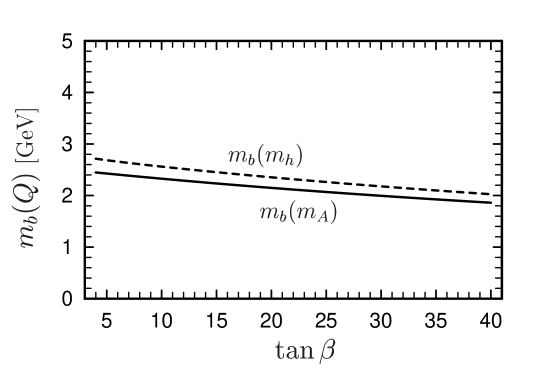
In the following we show the numerical improvement of the SUSY QCD corrections to the widths of Higgs boson decays to quarks and squarks. First we show in Fig. 1 the SUSY QCD running bottom quark mass at the scale of $h^{0}$, $m_{b}(m_{h})$ (dashed line), and at the scale of $A^{0}$, $m_{b}(m_{A})$ (full line), as a function of $\tan\beta$. The following values for the parameters are used: $(M_{\tilde{Q}}({\tilde{t}}),M_{\tilde{U}},M_{\tilde{D}})=(300,270,330)$ GeV, $A_{t}=150$ GeV, $A_{b}(Q)=-700$ GeV (where $Q=m_{h}$ or $m_{A}$), $m_{{\tilde{g}}}=350$ GeV, $\mu=260$ GeV, and $m_{A}=800$ GeV.

Figure 1: Running bottom mass as a function of $\tan\beta$. The on–shell value is $M_{b}=5$ GeV. Furthermore, $m_{b}(m_{h})_{\rm SM}\simeq 3.0$ GeV with $m_{h^{0}}=93$ to $103$ GeV, and $m_{b}(m_{A})_{\rm SM}=2.6$ GeV. The other parameters are given in the text.

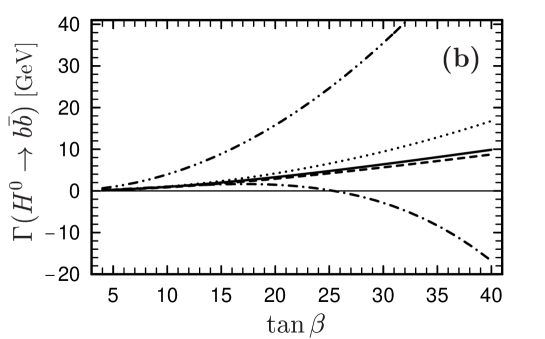
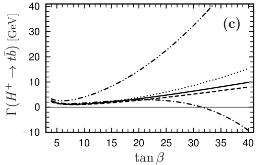
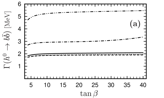
In Fig. 2 the tree–level and corrected widths of Higgs boson decays to bottom quarks are shown in two ways of perturbative expansion, (i) the strict on–shell scheme (dash–dot–dotted line: tree–level, dash–dotted line: one–loop corrected), and (ii) the improved scheme as discussed in section 3.2 (dashed: tree–level, full line: one–loop corrected), as a function of $\tan\beta$. The parameters used are the same as in Fig. 1 with $Q$ at the mass of the parent Higgs boson. (Notice that for case (i) $A_{b}=-700$ GeV is the on–shell value.) In addition, the tree–level decay width using (iii) the non–supersymmetric QCD running mass $m_{b}(m_{\phi})_{\rm SM}$ is shown (dotted line). One can clearly see that the difference between tree–level and corrected widths decreases dramatically from (i) to (ii), especially for decays of the heavier Higgs bosons $(H^{0},A^{0},H^{\pm})$. (The curves for $\Gamma(A^{0}\to b\bar{b})$ are practically the same as those for $\Gamma(H^{0}\to b\bar{b})$.) In particular, the physically meaningless “negative width” is absent for (ii). This demonstrates the improvement of the convergence of the SUSY QCD perturbation expansion by the method proposed in this paper. Furthermore, Fig. 2a shows that (iii) is indeed a good approximation for $h^{0}\to b\bar{b}$ in the large $m_{A}$ limit, Eq. (22). This is, however, not the case for the decays of the heavier Higgs particles to quarks, see the Figs. 2b and 2c.

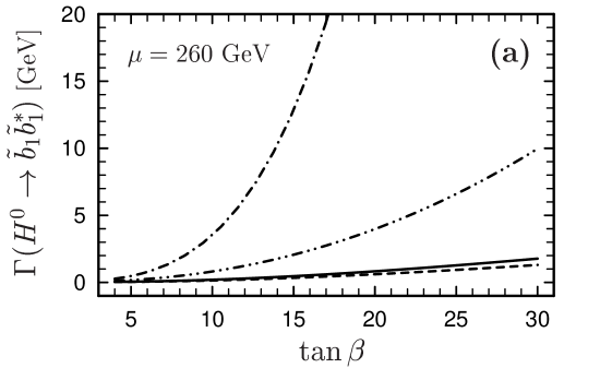
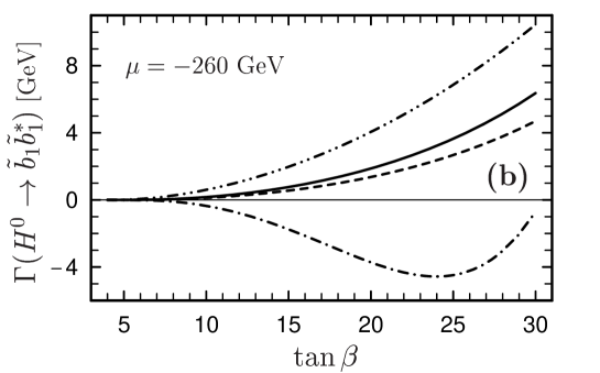
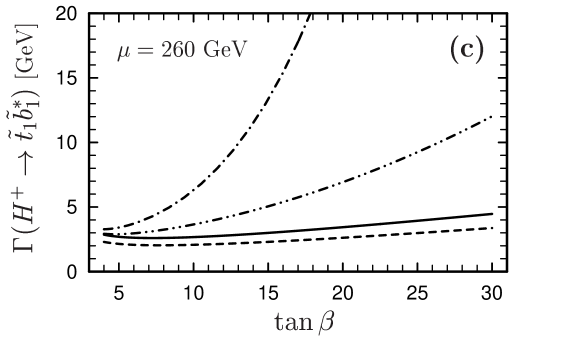
We next show the numerical improvement of the SUSY QCD corrections to the decay widths to squarks. Figure 3 shows the tree–level and corrected decay widths of $H^{0}\rightarrow{\tilde{b}}_{1}{\tilde{b}}_{1}^{*}$ for $\mu=260$ GeV and $-260$ GeV, and $H^{+}\rightarrow{\tilde{t}}_{1}{\tilde{b}}_{1}^{*}$ for $\mu=260$ GeV, as functions of $\tan\beta$. The other parameters are the same as in Fig. 2. We compare the strict on–shell perturbation expansion of [10] (i) and the improved one (ii) as described in section 4. The improvement of the perturbation expansion is again very clear. The results for $\Gamma(A^{0}\to{\tilde{b}}_{1}{\tilde{b}}_{2}^{*})$ are similar to those for $\Gamma(H^{0}\to{\tilde{b}}_{1}{\tilde{b}}_{1}^{*})$.

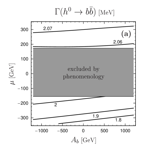
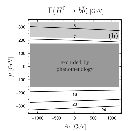
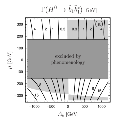
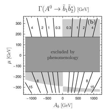
We now calculate the parameter dependence of the SUSY QCD corrected widths $\Gamma(h^{0}\rightarrow b\bar{b})$, $\Gamma(H^{0}\rightarrow b\bar{b})$, $\Gamma(H^{0}\rightarrow{\tilde{b}}_{1}{\tilde{b}}_{1}^{*})$, and $\Gamma(A^{0}\rightarrow{\tilde{b}}_{1}{\tilde{b}}_{2}^{*})$ for $\tan\beta=30$, which could not be presented in [8, 10] because the widths would have become negative. The results are shown in Figs. 4 and 5 as contour plots in the ($A_{b}(Q)$, $\mu$) plane for $\tan\beta=30$, with the SU(2) gaugino mass $M=117$ GeV, and the other parameters being the same as in Fig. 1.

As expected from Eq. (13), in Fig. 4 the corrections to $\Gamma(h^{0}\rightarrow b\bar{b})$ and $\Gamma(H^{0}\rightarrow b\bar{b})$ are mainly determined by $\mu$. Note also that the $\mu$ dependence is much stronger for $\Gamma(H^{0}\rightarrow b\bar{b})$ in Fig. 4b than for $\Gamma(h^{0}\rightarrow b\bar{b})$ in Fig. 4a, in accordance with the discussion in section 3.1.

As can be seen in Fig. 5a, the decay width of $H^{0}\rightarrow{\tilde{b}}_{1}{\tilde{b}}_{1}^{*}$ becomes large for large $|A_{b}(Q)|$ and/or large negative $\mu$. One can see that the tree–level invariance of the decay width under the sign change $(A_{b},\mu)\rightarrow(-A_{b},-\mu)$ is badly violated. This is due to the gluino loops.

Figure 2: Widths of Higgs particle decays into quarks as a function of $\tan\beta$. Case (i): dash–dot–dotted line corresponds to the on–shell tree–level, and dash–dotted to the on–shell one–loop result. Case (ii): dashed line corresponds to the improved tree–level, and full line to the improved one–loop result. Case (iii): dotted line corresponds to the tree–level result improved only by using $m_{b}(Q)_{\rm SM}$. For details, see the related text.

Figure 3: Widths of Higgs particle decays into squarks as a function of $\tan\beta$. Case (i): dash–dot–dotted line corresponds to the on–shell tree–level, and dash–dotted to the on–shell one–loop result. Case (ii): dashed line corresponds to the improved tree–level, and full line to the improved one–loop result. For details, see the related text.

Figure 4: Contour lines for the improved one–loop decay widths of Higgs particle decays into bottom quarks as a function of $A_{b}$ running and $\mu$. In (b) the light gray area shows the region where the on–shell one–loop result is negative. The other parameters are given in the text. The dark gray area is excluded by LEP and Tevatron data [28].

Figure 5: Contour lines for the improved one–loop decay widths of Higgs particles decay into bottom squarks as a function of $A_{b}$ running and $\mu$. The light gray areas show the region where the on–shell one–loop result is negative. The other parameters are given in the text. The dark gray area is excluded by LEP and Tevatron data [28].

Finally we comment on the $m_{{\tilde{g}}}$ dependence. It has been pointed out in [7, 9] that the gluino correction to quark modes decouples very slowly for increasing $m_{{\tilde{g}}}$ $(m_{{\tilde{g}}}>m_{{\tilde{q}}})$ with fixed squark parameters. This property can be understood from Eq. (13). The correction $\Delta_{b}$ scales as $(\ln m_{{\tilde{g}}})/m_{{\tilde{g}}}$ in this limit, decreasing much more slowly than the usual $1/M^{2}$ behavior.

6 Conclusion

The SUSY QCD corrections to the decays of MSSM Higgs bosons to quarks and squarks of the third gereration are phenomenologically very important. The existing formulae for the one–loop SUSY QCD corrections to their decay widths have been given in the on–shell expansion for quarks and squarks. However, for large $\tan\beta$, these formulae suffer from very bad convergence of the perturbation series, which makes the numerical results unreliable.

We have worked out a method for improving the SUSY QCD corrections to these widths. The essential point of the improvement is to define appropriate tree–level couplings of the Higgs bosons to quarks and squarks, in terms of the running quark masses $m_{q}(Q)$ both in non–SUSY and SUSY QCD, the running Higgs–squark trilinear couplings $A_{q}(Q)$, and the on–shell left–right mixing angle $\theta_{{\tilde{q}}}$ of squarks. We have also shown numerically that this method greatly improves the corrections to the decays to bottom quarks and squarks.

We finally note that the method of improvement for the Higgs boson couplings to quarks and squarks as presented in this paper is also useful in studying radiative corrections to other processes, such as the decays of a squark into chargino/neutralino and quark [32, 22], those into lighter squark and Higgs boson [11, 12], low energy four–fermi interactions with virtual charged Higgs boson [33], and associated production of Higgs bosons with quarks [34] and squarks [35].

References

• [1] For reviews, see:
H.P. Nilles, Phys. Rep. 110 (1984) 1;
H.E. Haber and G.L. Kane, Phys. Rep. 117 (1985) 75;
R. Barbieri, Riv. Nuov. Cim. 11 (1988) 1.
• [2] J.F. Gunion and H.E. Haber, Nucl. Phys. B272 (1986) 1; B402 (1993) 567 (E).
• [3] A. Djouadi, J. Kalinowski, and P.M. Zerwas, Z. Phys. C 70 (1996) 435.
• [4] A. Bartl, K. Hidaka, Y. Kizukuri, T. Kon, and W. Majerotto, Phys. Lett. B 315 (1993) 360;
A. Bartl, H. Eberl, K. Hidaka, T. Kon, W. Majerotto, and Y. Yamada, Phys. Lett. B 389 (1996) 538.
• [5] A. Djouadi, J. Kalinowski, P. Ohmann, and P.M. Zerwas, Z. Phys. C 74 (1997) 93.
• [6] A. Dabelstein, Nucl. Phys. B 456 (1995) 25.
• [7] J.A. Coarasa, R.A. Jiménez, and J. Solà, Phys. Lett. B 389 (1996) 312.
• [8] A. Bartl, H. Eberl, K. Hidaka, T. Kon, W. Majerotto, and Y. Yamada, Phys. Lett. B 378 (1996) 167.
• [9] R.A. Jiménez and J. Solà, Phys. Lett. B 389 (1996) 53.
• [10] A. Bartl, H. Eberl, K. Hidaka, T. Kon, W. Majerotto, and Y. Yamada, Phys. Lett. B 402 (1997) 303.
• [11] A. Arhrib, A. Djouadi, W. Hollik, and C. Jünger, Phys. Rev. D 57 (1998) 5860.
• [12] A. Bartl, H. Eberl, K. Hidaka, S. Kraml, W. Majerotto, W. Porod, and Y. Yamada, Phys. Rev. D 59 (1999) 115007.
• [13] E. Braaten and J.P. Leveille, Phys. Rev. D 22 (1980) 715;
M. Drees and K. Hikasa, Phys. Lett. B 240 (1990) 455; 262 (1991) 497 (E);
A. Méndez and A. Pomarol, Phys. Lett. B 252 (1990) 461.
• [14] S.G. Gorishny, A.L. Kataev, S.A. Larin, and L.R. Surguladze, Mod. Phys. Lett. A5 (1990) 2703; Phys. Rev. D 43 (1991) 1633;
A. Djouadi, M. Spira, and P.M. Zerwas, Z. Phys. C 70 (1996) 427;
A. Djouadi, J. Kalinowski, and M. Spira, Comput. Phys. Commun. 108 (1998) 56;
M. Spira, Fortschr. Phys. 46 (1998) 203.
• [15] R. Hempfling, Phys. Rev. D 49 (1994) 6168;
L.J. Hall, R. Rattazzi, and U. Sarid, Phys. Rev. D 50 (1994) 7048;
M. Carena, M. Olechowski, S. Pokorski, and C.E.M. Wagner, Nucl. Phys. B426 (1994) 269;
D.M. Pierce, J.A. Bagger, K. Matchev, and R. Zhang, Nucl. Phys. B491 (1997) 3.
• [16] M. Carena, S. Mrenna, and C.E.M. Wagner, Phys. Rev. D 60 (1999) 075010;
hep-ph/9907422.
• [17] P.H. Chankowski and S. Pokorski, hep-ph/9707497, in Perspectives on Supersymmetry, ed. by G. L. Kane (World Scientific, 1997);
K.S. Babu and C. Kolda, Phys. Lett. B 451 (1999) 77.
• [18] G. Passarino and M. Veltman, Nucl. Phys. B160 (1979) 151.
• [19] A. Denner, Fortschr. Phys. 41 (1993) 307.
• [20] J.A. Coarasa, D. Garcia, J. Guasch, R.A. Jiménez, and J. Solà, Phys. Lett. B 425 (1998) 329.
• [21] H. Eberl, A. Bartl, and W. Majerotto, Nucl. Phys. B 472 (1996) 481.
• [22] W. Beenakker, R. Höpker, T. Plehn, and P.M. Zerwas, Z. Phys. C 75 (1997) 349.
• [23] J. Guasch, J. Solà, and W. Hollik, Phys. Lett. B 437 (1998) 88;
H. Eberl, S. Kraml, and W. Majerotto, JHEP 9905 (1999) 016.
• [24] Y. Yamada, Phys. Rev. D 54 (1996) 1150.
• [25] D. Pierce and A. Papadopoulos, Nucl. Phys. B430 (1994) 278.
• [26] Y. Okada, T. Yanagida, and M. Yamaguchi, Prog. Theor. Phys. 85 (1991) 1; Phys. Lett. B 262 (1991) 54;
H. Haber and R. Hempfling, Phys. Rev. Lett. 66 (1991) 1815;
J. Ellis, G. Ridolfi, and F. Zwirner, Phys. Lett. B 257 (1991) 83.
• [27] M. Carena, M. Quirós, and C.E.M. Wagner, Nucl. Phys. B 461 (1996) 407.
• [28] A. Blondel, talk given at the CERN LEPC meeting, 9 Nov. 1999. For transparencies see http://alephwww.cern.ch/ALPUB/seminar/lepc_nov99/lepc.pdf;
A. Savoy–Navarro, talk at the International Europhysics Conference on High Energy Physics (HEP99), 15. – 21. July 1999, Tampere, Finland. For transparencies see http://neutrino.pc.helsinki.fi/hep99/Transparencies/session-07/Savoy-Navarro.pdf.
• [29] G. Altarelli, R. Barbieri, and F. Caravaglios, Int. J. Mod. Phys. A 13 (1998) 1031.
• [30] M. Drees and K. Hagiwara, Phys. Rev. D 42 (1990) 1709.
• [31] J.P. Derendinger and C.A. Savoy, Nucl. Phys. B 237 (1984) 307.
• [32] S. Kraml, H. Eberl, A. Bartl, W. Majerotto, and W. Porod, Phys. Lett. B 386 (1996) 175;
A. Djouadi, W. Hollik, and C. Jünger, Phys. Rev. D 55 (1997) 6975.
• [33] J.A. Coarasa, R.A. Jiménez, and J. Solà, Phys. Lett. B 406 (1997) 337.
• [34] Z. Kunszt, Nucl. Phys. B247 (1984) 339;
A. Djouadi, J. Kalinowski, and P.M. Zerwas, Z. Phys. C 54 (1992) 255; Mod. Phys. Lett. A7 (1992) 1765;
J. Kalinowski and M. Krawczyk, Phys. Lett. B 361 (1995) 66;
S. Dawson and L. Reina, Phys. Rev. D 60 (1999) 015003;
B. Grwadkowski, J.F. Gunion, and J. Kalinowski, Phys. Rev. D 60 (1999) 075011;
F. Borzumati, J.-L. Kneur, and N. Polonsky, Phys. Rev. D 60 (1999) 115011.
• [35] A. Djouadi, J.L. Kneur, and G. Moultaka, Phys. Rev. Lett. 80 (1998) 1830;
Nucl. Phys. B 569 (2000) 53;
G. Bélanger, F. Boudjema, T. Kon, and V. Lafage, Eur. Phys. J. C 9 (1999) 511;
A. Dedes and S. Moretti, Phys. Rev. D 60 (1999) 015007; Eur. Phys. J. C 10 (1999) 515;
G. Bélanger, F. Boudjema, and K. Sridhar, Nucl. Phys. B 568 (2000) 3.