SOLVING THE HIERARCHY PROBLEM WITH EXPONENTIALLY LARGE DIMENSIONS
Nima Arkani-Hamed, Lawrence Hall, David Smith and Neal Weiner
Department of Physics, University of California, Berkeley, CA 94530, USA
Theory Group, Lawrence Berkeley National Laboratory, Berkeley, CA 94530, USA
ABSTRACT

In theories with (sets of) two large extra dimensions and supersymmetry in the bulk, the presence of non-supersymmetric brane defects naturally induces a logarithmic potential for the volume of the transverse dimensions. Since the logarithm of the volume rather than the volume itself is the natural variable, parameters of O(10) in the potential can generate an exponentially large size for the extra dimensions. This provides a true solution to the hierarchy problem, on the same footing as technicolor or dynamical supersymmetry breaking. The area moduli have a Compton wavelength of about a millimeter and mediate Yukawa interactions with gravitational strength. We present a simple explicit example of this idea which generates two exponentially large dimensions. In this model, the area modulus mass is in the millimeter range even for six dimensional Planck scales as high as 100 TeV.

1 Introduction

It has recently been realized that the fundamental scales of gravitational and string physics can be far beneath $\sim 10^{18}$ GeV, in theories where the Standard Model fields live on a 3-brane in large-volume extra dimensions [1]. Lowering these fundamental scales close to the weak scale provides a novel approach to the hierarchy problem, and implies that the structure of quantum gravity may be experimentally accessible in the near future.

While this prospect is very exciting, two important theoretical issues need to be addressed for this scenario to be as compelling as the more “standard” picture with high fundamental scale, where the hierarchy is stabilized by SUSY dynamically broken at scales far beneath the string scale. First: what generates the large volume of the extra dimensions? And second: what about the successful picture of logarithmic gauge coupling unification in the supersymmetric standard model? The success is so striking that we do not wish to think it is an accident.

One way of generating a large volume for the extra dimensions involves considering a highly curved bulk. Indeed Randall and Sundrum have proposed a scenario where the bulk volume can be exponentially larger than the proper size of a single extra dimension [2]. Goldberger and Wise then showed how such a dimension could be stabilized [3]. In the original proposal of [1], however, the bulk was taken to be very nearly flat. Previous attempts at stabilizing large dimensions in this framework involved the introduction of large integer numbers in the theory, such as large topological charges [4, 5] or large numbers of branes [5]. In this paper, we instead demonstrate how to stabilize exponentially large dimensions in the framework of [1].

The set-up needed to accomplish this meshes nicely with recent discussions of how the success of logarithmic gauge coupling unification can be maintained with large dimensions and low string scale. In [6, 7, 8, 9, 10] it was argued that logarithmic gauge coupling unification may be reproduced in theories with (sets of) two large dimensions. If various light fields propagate in effectively two transverse dimensions, then the logarithmic Green’s functions for these fields can give rise to logarithmic variation of the parameters on our brane universe; in cases with sufficient supersymmetries, this logarithmic variation can exactly reproduce the logarithmic running of couplings seemingly far above the (now very low) string scale. This phenomena is another example of the bulk reproducing the physics of the desert, this time with quantitative precision. Of course, for the “infrared running” picture to work after SUSY breaking, we must assume that SUSY is not broken in the bulk but only directly on branes. This is the analogue of softly breaking SUSY at low energies in the usual desert picture.

It is interesting that these same ingredients: sets of two transverse dimensions with SUSY in the bulk, only broken on branes, can also be used to address the issue of large radius stabilization. Indeed, in the SUSY limit, there is no bulk cosmological constant and there is no potential for the radii; they can be set at any size. The crucial point is that once SUSY is broken on branes with a characteristic scale $\Lambda^{4}$, locality guarantees that no bulk cosmological constant is induced, and therefore the effective potential for the radius moduli does not develop any positive power-law dependence on the volume of the transverse dimensions. For two transverse dimensions, logarithmic variation of light bulk fields can then give rise to a logarithmic potential for the size, $R$, of the extra dimensions:

$$V(R)\sim\Lambda^{4}f(\mbox{log}(RM_{*}))$$ (1)

where $M_{*}$ is the fundamental scale of the theory. This can arise, for instance, from the infrared logarithmic variation of coupling constants on branes where SUSY is broken or from inter-brane forces [7, 10, 11]. Since $\log(R)$ rather $R$ itself is the natural variable, if the potential has parameters of $O(10)$, a minimum can result at log$({\overline{R}})\sim 10$, thereby generating an exponentially large radius and providing a genuine solution to the hierarchy problem, on the same footing as technicolor or dynamical SUSY breaking.

This idea is appealing and general; relying only on sets of two transverse dimensions (for the logarithmic dependence) and supersymmetry in the bulk (to stably guarantee the absence of a bulk constant which would induce power-law corrections to the effective potential for the radii). It makes the existence of large extra dimensions seem plausible. However, the discussions in [7, 10, 11] have only pointed out this possibility on general grounds but have not presented concrete models realizing the idea. In this paper we remedy this situation by presenting an explicit example of a simple theory with two extra dimensions, which stabilizes exponentially large dimensions. The interaction of branes with massless bulk scalar fields induces a logarithmic potential for the area $A$ of the transverse dimensions of the form

$$V(A)=-f^{4}+\frac{v^{4}}{\mbox{log}(AM_{*}^{2})}+w^{4}\mbox{log}(AM_{*}^{2}).$$ (2)

This potential is minimized for an area

$${\overline{A}}M_{*}^{2}=e^{v^{2}/w^{2}}$$ (3)

and so only a ratio of $v/w\sim 6$ is needed to generate an area to generate the $\sim($mm$)^{2}$ area needed to solve the hierarchy problem with $M_{*}\sim$ TeV. There is a single fine-tuning among the parameters $v,w$ and $f$, which are all of order $M_{*}$, to set the 4D cosmological constant to zero.

2 The Radion Signal

Since the potential for the radii of the extra dimensions vary only logarithmically, one might worry that the mass of the radius modulus about the minimum of the potential will be too light. In fact, the mass turns out to be just in the millimeter range, and gives an observable deviation from Newton’s law at sub-millimeter distances.

Consider a 6 dimensional spacetime with metric of the form

$$ds^{2}=g_{\mu\nu}(x)dx^{\mu}dx^{\nu}+R^{2}(x)\tilde{g}(y)_{mn}dy^{m}dy^{n},$$ (4)

where the geometry of $\tilde{g}$ is taken to be fixed at high energy scales; for example by brane configurations, as illustrated in the next section. The low energy 4D effective field theory involves the 4D graviton together with the radion field, $R(x)$, which feels the potential of eq. (1). After a Weyl rescaling of the metric to obtain canonical kinetic terms, the radion is found to have a mass

$$m^{2}_{R}\sim\frac{R^{2}V^{\prime\prime}(R)}{M_{Pl}^{2}}\sim\frac{\Lambda^{4}}{M_{Pl}^{2}}f^{\prime\prime}(\mbox{log}{R})\sim\left(\frac{\mbox{TeV}^{2}}{M_{Pl}}\right)^{2}\sim\mbox{mm}^{-2}.$$ (5)

Hence, an interesting general consequence of such logarithmic potentials is that the mass of the radion is naturally in the millimeter range for supersymmetry breaking and fundamental scales $\Lambda\sim M_{*}\sim$TeV. This order of magnitude result is important for mm range gravity experiments, because the Weyl rescaling introduces a gravitational strength coupling of the radion to the Standard Model fields, so that radion exchange modifies the Newtonian potential to

$$V(r)=-{G_{N}m_{1}m_{2}\over r}\;(1+2e^{-m_{R}r}).$$ (6)

For a radion which determines the size of an $n$ dimensional bulk, the coefficient of the exponential is $4n/(n+4)$, so that an observation of a coefficient corresponding to $n=2$ would be a dramatic signal of our mechanism.

It might be argued that, since $M_{*}$ is larger than 50–100 TeV for $n=2$ from astrophysics and cosmology ([12, 13]), $m_{R}$ will be sufficiently large that the range of the radion-mediated force will be considerably less than than a mm, making an experimental discovery extremely difficult. This conclusion is incorrect, for several reasons:

• The astrophysical and cosmological limits are derived from graviton emission and hence constrain the gravitational scale, which may be somewhat larger than the fundamental scale, $M_{*}$.

• It is the scale of supersymmetry breaking on the branes, $\Lambda$, which determines $m_{R}$, and this may be less than $M_{*}$, reducing $m_{R}$ and making the range of the Yukawa potential larger.

• The radion mass may be reduced from the order of magnitude estimate $m_{R}\approx\Lambda^{2}/M_{Pl}$ by powers of log $R$, depending on the function $f$ which appears in the potential (1), as occurs in the theory described in the next section.

• Finally, the cosmological and astrophysical limits on the fundamental scale are unimportant in the case that the bulk contains more than one 2D subspace, but as discussed in section 4, the radions still have masses $\sim$ mm^-1.

3 Explicit model

In this section we present a specific effective theory that stabilizes two large extra dimensions, without relying on input parameters with particularly large ($>10$) ratios. The framework for our model is as follows. Supersymmetry in the bulk guarantees a vanishing bulk cosmological constant. Embedded in the 6D spacetime is a set of parallel three-branes that can be regarded as non-supersymmetric defects. Following closely the example of [4], the tensions of these three-branes themselves compactify the extra dimensions. We take the bulk bosonic degrees of freedom to be those of the supergravity multiplet, namely, the graviton $g_{AB}$ and the anti-self-dual 2-form $A_{AB}$. The 2-form $A_{AB}$ does not couple to any of the three-branes and can be set to zero in our case. We can also have a set of massless bulk scalars $\phi_{i}$ contained in hypermultiplets. The relevant part of the Bosonic action is then

$$S=S_{Bulk}+S_{Brane}$$ (7)

where

$$S_{Bulk}=\int d^{4}xd^{2}y\sqrt{-G}\left(-2M^{4}R+\sum_{i}(\partial\phi_{i})^{2}+\cdots\right)$$ (8)

is the bulk action and

$$S_{Branes}=\int d^{4}x\sum_{i}\sqrt{-g_{i}}\left(-f_{i}^{4}+\sum_{a}{\cal L}_{a}(\psi_{a},\phi|_{a})+\cdots\right)$$ (9)

is the action for the branes [14]. Here the $f_{i}^{4}$ are the brane tensions and ${\cal L}_{i}$ are Lagrangians for fields $\psi_{i}$ that may live on the branes, which can also depend on the value of bulk fields $\phi$ evaluated on the brane $\phi|_{a}$. $G$ is the 6d metric, $g_{i}$ is the induced metric on the $i$’th brane, and we have set the bulk cosmological constant to zero.

Note that while $S_{Bulk}$ must be accompanied by all the extra fermionic terms to have SUSY in the bulk, the brane actions do not have to linearly realize SUSY at all, although they may realize SUSY non-linearly. In particular, there need not be any trace of superpartners on the brane where the Standard Model fields reside. The only reason we need SUSY in the bulk is to protect against the generation of a bulk cosmological constant $\Lambda_{bulk}$, which would make a contribution $\sim\Lambda_{bulk}A$ to the potential for the area modulus and spoil our picture with logarithmic potentials.

Our model has three 3-branes, two of which couple to scalars $\phi$ and $\phi^{\prime}$. The dynamics on the brane impose boundary conditions on the bulk scalar fields. In particular, imagine that the the brane defects create brane-localized potentials for $\phi$, which want $\phi$ to take on the value $v_{1}^{2}$ on one brane and $v_{2}^{2}$ on the other. This will lead to a repulsive contribution to the potential for the area. The same two branes will be taken to have equal and opposite magnetic charges for the scalar $\phi^{\prime}$, setting up a vortex-antivortex configuration for $\phi^{\prime}$ which will lead to an attractive potential. The balance between these contributions provides a specific realization of how competing dependences on $\log R$ can lead to an exponentially large radius without very large or small input parameters.

We begin by reviewing how the brane tensions can compactify the two extra dimensions [14, 15]. Suppose we ignore for the time being the branes’ couplings to bulk scalars, in which case the relevant terms in the action in the low-energy limit are

$$S=-\int d^{4}x\sum_{i}\sqrt{-g_{i}}{f_{i}}^{4}-2M^{4}\int d^{4}xd^{2}y\sqrt{-G}R.$$ (10)

For the case in which only a single brane is present, the static solution to Einstein’s equations is

$$ds^{2}=\eta_{\mu\nu}dx^{\mu}dx^{\nu}+{\cal G}_{mn}(y)dy^{m}dy^{n},$$ (11)

where ${\cal G}_{mn}$ is the 2D Euclidean metric everywhere but at the position of the three-brane, where it has a conical singularity with deficit angle

$$\delta={f^{4}\over 4M^{4}}.$$ (12)

As expected, this is in exact correspondence with the metric around point masses in 2+1 dimensional gravity [15]. As shown in Figure 1, the spatial dimensions transverse to the brane are represented by the Cartesian plane with a wedge of angle $\delta$ removed.

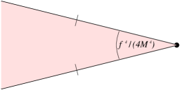
Figure 1: The two transverse dimensions in the presence of a three-brane with tension $f^{4}$. The shaded region is excluded, and the two borders of the excluded region are to be identified.

Adding a second brane removes a further portion of the Cartesian plane. In fact, if ${f_{1}^{4}\over 4M^{4}}+{f_{2}^{4}\over 4M^{4}}>2\pi$, then the excluded region surrounds the allowed portion, as in Figure 2.

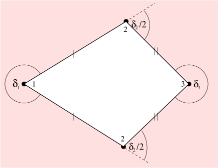
Figure 2: A compact space can be obtained given three branes whose corresponding deficit angles $\delta_{i}$ add up to $4\pi$. Identifications to be made are indicated by hash marks. Note that in contrast to the brane in Figure 1, branes 1 and 3 in this figure have tensions larger than $4\pi M^{4}$.

In this case Einstein’s equations have a static solution that features a compact space with spherical topology, provided that a third brane of tension $f_{3}^{4}=16\pi M^{4}-f_{1}^{4}-f_{2}^{4}$ is placed at the intersecting lines of exclusion. In general, a set of three-branes has a static solution with spherical topology if

$$\sum_{i}{f_{i}^{4}\over 4M^{4}}=4\pi,$$ (13)

that is, the deficit angles must add up to 4$\pi$.

If a set of branes compactifies the space in this manner, then the 4D effective theory is given by including in the action of (10) the massless excitations about the classical metric. Thus we replace $\eta_{\mu\nu}\rightarrow{\overline{g}}_{\mu\nu}(x)$ and allow ${\cal G}_{mn}(y)$ to fluctuate about $\delta_{mn}$ in the bulk. The induced metric on a given brane will differ from ${\overline{g}}_{\mu\nu}(x)$ by terms involving the fields associated with the brane separations, which we temporarily ignore. The curvature breaks up into two pieces $R^{(4)}$ and $R^{(2)}$, the Ricci scalars built out of ${\overline{g}}_{\mu\nu}(x)$ and ${\cal G}_{mn}(y)$, respectively. Then, using the Gauss-Bonnet Theorem for spherical topology,

$$\int d^{2}y\sqrt{{\cal G}}R^{(2)}=-8\pi,$$ (14)

along with the fact that $R^{(4)}$ has no $y$ dependence, we can integrate over the extra dimensions to obtain

$$S=-\int d^{4}x\sqrt{-\overline{g}}\left(\sum_{i}f_{i}^{4}-16\pi M^{4}+2(\int d^{2}y\sqrt{{\cal G}})M^{4}R^{(4)}\right).$$ (15)

In this action it is explicit that adjusting the deficit angles to add up to $4\pi$ is equivalent to tuning the 4D cosmological constant to zero.

To develop our specific model we consider the case of three three-branes on a space of spherical topology. Then the “shape” of the extra dimensions is fixed by the branes’ deficit angles, or equivalently, by their tensions. However, the size of the extra dimensions,

$$A=\int d^{2}y\sqrt{{\cal G}},$$ (16)

is completely undetermined. Moreover, the scalar associated with fluctuations of $A$, the radion, is massless and mediates phenomenologically unacceptable long-range forces. To stabilize the volume of the extra dimensions and give the radion a mass, we couple bulk scalar fields to two of the branes, which, for simplicity, we assume have equal tensions $f$. The scalar profiles will generate a potential $V_{\phi}(A)$ that is minimized for a certain value $\overline{A}$ of the volume of the compactified space. Adding the scalar action to (15) yields a total potential

$$V(A)=V_{\phi}(A)+\sum_{i}f_{i}^{4}-16\pi M^{4}.$$ (17)

The effective cosmological constant,

$$\Lambda_{eff}=V(\overline{A}),$$ (18)

can then be made to vanish by a single fine tuning of fundamental parameters. The back-reaction on the spatial geometry that is induced by the scalars is discussed below.

We work with two massless bulk scalars, $\phi$ and $\phi^{\prime}$, which induce repulsive and attractive forces, respectively. In treating the scalar fields, we will for simplicity ignore their back-reaction on the metric and assume that they propagate in the flat background with conical singularities set up by the branes. It is easy to see that the effect of back-reaction can be made parametrically small if the scalar energy scales are somewhat smaller than $M_{*}$, and none of our conclusions are affected.

Suppose that on branes 1 and 3 of Figure 3,

Figure 3: The boundary conditions on $\phi$. Identifications to be made are indicated by hash marks.

$\phi$ is forced to take on unequal values $v^{2}_{1}$ and $v^{2}_{3}$, respectively. This can for instance be enforced if the non-SUSY brane defects generate a potential for $\phi$ on the branes, analogous to what was considered in [3]. Because $\phi$ is massless in the bulk, we are free to perform a constant field redefinition and take $v^{2}_{1}=-v^{2}_{3}\equiv v^{2}$. We account for the brane thicknesses by enforcing these values for $\phi$ to hold along arcs of finite radius $r_{*}\sim 1/M_{*}$, and not just at individual points. The field configuration in the bulk is then given by solving Laplace’s equation with these boundary conditions.

Keeping in mind the identifications to be made between the various edges of the space in Figure 3, the symmetry of the problem tells us that the field configuration is found by solving the problem depicted in Figure 4, and then reflecting that solution appropriately.

Figure 4: A boundary-value problem that determines $\phi$. Here ${\mathbf{e}}_{\bot}$ refers to the unit vector normal to the relevant boundary, and lines of ${\mathbf{\nabla}\phi}$ are shown dashed. The solution for the full space of Figure 3 is given by first evenly reflecting across the bottom horizontal line, and then performing an odd reflection (i.e., $\phi\rightarrow-\phi$) across the vertical line where $\phi=0$.

For simplicity we consider instead a slightly different problem which, unlike that shown in Figure 4, is trivially solved.

Figure 5: The simplified boundary-value problem for $\phi$.

As indicated in Figure 5, we take the boundary at which $\phi=0$ holds to be an arc of radius $R$, rather than a straight line, so that the solution in this region is immediately found to be

$$\phi=v^{2}{\log{(R/r)}\over\log{(R/r_{*})}},$$ (19)

where $r$ measures the distance from the (missing) left vertex of the pie slice. The total energy of this configuration is

$$4\int d\theta\int_{r_{*}}^{R}drr{({\mathbf{\nabla}}\phi)^{2}\over 2}=\theta_{0}{v^{4}\over\log{(R/r_{*})}},$$ (20)

where $\theta_{0}=2\pi-{f^{4}\over 4M^{4}}$. Thus, $\phi$ sets up a $1/\log{R}$ repulsive potential. It is not difficult to prove using simple variational arguments that the same conclusion is reached when one solves the “real” problem involving the triangle rather than the pie slice.

Now suppose that the same two branes that couple to $\phi$ carry topological charge under a derivatively coupled field $\phi^{\prime}$. That is, under any closed loop containing a brane we have

$$\int{\mathbf{d}}{\mathbf{l}}\cdot{\mathbf{\nabla}}\phi^{\prime}=n\theta_{0}w^{2},$$ (21)

where $w$ is a fixed parameter with unit mass dimension and $n$ is an integer. Non-zero charge $n\neq 0$ is only possible if we make the identification

$$\phi\sim\phi+\theta_{0}w^{2}.$$ (22)

In order to be able to solve Laplace’s equation on a compact space, the branes must carry equal and opposite charges, which we take to correspond to $n=\pm 1$. The configuration for $\phi^{\prime}$ is then found by solving Laplace’s equation with ${\mathbf{\nabla}}\phi^{\prime}=\pm{w^{2}\over r_{*}}\mathbf{e_{\|}}$ on the branes (the gradient runs clockwise on one brane and counterclockwise on the other). This sets up the the vortex-antivortex field configuration for $\phi^{\prime}$ shown in Figure 6.

Figure 6: The configuration of $\phi^{\prime}$. Each brane carries a topological charge, which generates an attractive potential.

For simplicity, in order to calculate the energy in this configuration we once again work on a pie slice (Figure 7)

Figure 7: The simplified boundary-value problem for $\phi^{\prime}$ . Here $\mathbf{e_{\bot}}$ and $\mathbf{e_{\|}}$ are the unit vectors normal and parallel, respectively, to the relevant boundary.

rather than a triangle, and it is easily proved that this modification does not affect the essential scaling of the energy with the area. With this simplification the solution is

$$\phi^{\prime}=w^{2}\theta+C,$$ (23)

where $\theta$ is the angular coordinate and $C$ is an undetermined, irrelevant constant. The energy of the configuration is then found to be

$$4\int d\theta\int_{r_{*}}^{R}drr{({\mathbf{\nabla}}\phi^{\prime})^{2}\over 2}=\theta_{0}w^{4}\mbox{log}(R/r_{*}).$$ (24)

so we have found an attractive potential that will balance the repulsive contribution of (20). ¿From (20) and (24), we see that the full potential is

$$V(R)=\theta_{0}{v^{4}\over\log(R/r_{*})}+\theta_{0}w^{4}\log(R/r_{*})+\sum_{i}f_{i}^{4}-16\pi M^{4},$$ (25)

which is minimized when

$$R=\bar{R}=r_{*}e^{v^{2}/w^{2}}.$$ (26)

Even a mild ratio $v/w\sim 6$ yields an exponentially large radius $\bar{R}\sim 10^{16}r_{*}$. The effective cosmological constant,

$$\Lambda_{eff}=V(\bar{R})=\sum_{i}f_{i}^{4}-16\pi M^{4}+2\theta_{0}v^{2}w^{2},$$ (27)

can be made to vanish by a single tuning of $v$, $w$, and the brane tensions.

Note that we can now see explicitly that the presence of the non-supersymmetric brane defects can not generate a bulk cosmological constant. The presence of the branes leads to logarithmic variation for the bulk fields, which does indeed break SUSY and generate a potential for the area modulus. However, since any constant field configuration preserves SUSY, the SUSY breaking in the bulk must be proportional to the gradient of the bulk scalar fields, which drops as $1/r$ with distance $r$ away from the branes. Therefore, it is impossible to induce a cosmological constant, since this would amount to an constant amount of SUSY breaking throughout the bulk. In fact, a very simple power-counting argument shows that all corrections to the energy are logarithmic functions of the area.

Given a specific form for the logarithmic potential (25), we can work out the mass of the area modulus, which is

$$m^{2}_{R}\sim\frac{\bar{R}^{2}V^{\prime\prime}(\bar{R})}{M_{Pl}^{2}}\sim\frac{v^{4}}{M_{Pl}^{2}\mbox{log}^{3}(\bar{R}/r_{*})}.$$ (28)

Interestingly, $m_{R}$ is suppressed by (log$(\bar{R}/r_{*}))^{3/2}$ compared to the naive estimate $M_{*}^{2}/M_{Pl}$. Hence even for $v\sim M_{*}$ as large as 100 TeV, the range of the radion-mediated Yukawa potential is 0.1 mm – accessible to planned experiments.

4 Four and Six Extra Dimensions

Since the logarithmic form of the propagator occurs only in two dimensions, one may worry that the ideas in this paper are only applicable to the case of two large dimensions. This is the case most severely constrained by astrophysical and cosmological constraints [1, 12, 13], which demand the 6D Planck scale $M_{*}>$ 50 TeV, seemingly too large to truly solve the hierarchy problem. One possibility is that the true Planck scale of the ten dimensional theory could be $\sim$ O(TeV), and the 6D Planck scale of $\sim 50$ TeV could arise if the remaining four dimensions are a reasonable factor $O(10)$ bigger than a (TeV$)^{-1}$. But we don’t have to resort to this option. As pointed out in [7, 10], the presence of two-dimensional subspaces where massless fields can live is sufficient to generate logarithms. Take the case of four extra dimensions. Imagine one set of parallel 5-branes filling out the 12345 directions, and another set filling out the 12367 directions. They will intersect on 3-dimensional spaces where 3-branes can live. These 3-branes can act as sources for fields living on each of the 5-branes, which effectively propagate in two sets of orthogonal 2D subspaces. Once again, bulk SUSY can guarantee a vanishing “cosmological constant” for each of the 2D subspaces. The SUSY breaking at the intersections can set up logarithmically varying field configurations on the 5-branes that leads to a potential of the form $V(\mbox{log}A_{1},\mbox{log}A_{2})$ for the areas $A_{1},A_{2}$ of the 2D subspaces. Minimizing the potential, each radius can be exponentially large, and the ratio of the radii will also be exponential, but the value of $M_{Pl}$ will require the largest radius to be very much smaller than a mm. It would be interesting to build an explicit model along these lines.

Even without an explicit model, however, we can see that the scale of the radion masses is unchanged. The logarithmic potential still gives $m_{Ri}\approx\Lambda^{2}/M_{Pl}\approx\mbox{mm}^{-1}$, for $\Lambda\approx 1$ TeV. After Weyl rescaling, each radion couples with gravitational strength to the Standard Model and should show up in the sub-millimeter measurements of gravity.

5 Other ideas

There is an alternative way in which theories with two transverse dimensions can generate effectively exponentially large radii. The logarithmic variation of bulk fields can force the theory into a strong-coupling region exponentially far away from some branes, and interesting physics can happen there. This is the bulk analog of the dimensional transmutation of non-Abelian gauge theories, which generate scales exponentially far beneath the fundamental scale and trigger interesting physics, such as e.g. dynamical supersymmetry breaking [10]. It is tempting to speculate that such strong-coupling behavior might effectively compactify the transverse two dimensions. Recently, Cohen and Kaplan have found an explicit example realizing this idea [16]. They consider a massless scalar field with non-trivial winding in two transverse dimensions: a global cosmic string. Since the total energy of the string diverges logarithmically with distance away from the core of the vortex, we expect gravity to become strongly coupled at exponentially large distances. Indeed, Cohen and Kaplan find that the metric develops a singularity at a finite proper distance from the vortex core, but argue that the singularity is mild enough to be rendered harmless. What they are left with is a non-compact transverse space, with gravity trapped to an exponentially large area

$$\bar{A}M_{*}^{2}=e^{M_{*}^{4}/f_{\pi}^{4}}$$ (29)

where $f_{\pi}$ is the decay constant of the string. A ratio of $M_{*}/f_{\pi}\sim 2.5$ is all that is needed to solve the hierarchy problem in this case. This model is a natural implementation of the ideas of [1], to solve the hierarchy problem with large dimensions, together with the idea of trapping gravity in non-compact extra dimensions as in [17]. Unlike [2], however, the bulk geometry is not highly curved everywhere, but only near the singularity. Thus, gravity has essentially been trapped to a flat “box” of area $A$ in the transverse dimensions, and the phenomenology of this scenario is essentially the same as that of [1]. An attractive aspect of this scenario is that, unlike both our proposal in this paper and those of [2, 3], no modulus needs to be stabilized in order to solve the hierarchy problem. This also points to a phenomenological difference between our proposal and that of [16]. While both schemes generate an exponentially large area for two transverse dimensions, there is no light radion mode in [16] whereas we have a light radion with $\sim$mm^-1 mass.

6 Conclusions

In this paper, we have shown how to stabilize exponentially large compact dimensions, providing a true solution to the hierarchy problem along the lines of [1] which is on the same footing as technicolor and dynamical SUSY breaking. Of course, there are many mysteries other than the hierarchy problem, and the conventional picture of beyond the Standard Model physics given by SUSY and the great desert had a number of successes. So why do we bother pursuing alternatives? Are we to think that the old successes are just an accident?

A remarkable feature of theories with large extra dimensions is that the phenomena that used to be understood inside the energy desert can also be interpreted as arising from the space in the extra dimensions. Certainly all the qualitative successes of the old desert, such as explaining neutrino masses and proton stability, can be exactly reproduced with the help of the bulk [1, 19, 20, 18], in such a way that e.g. the success of the see-saw mechanism in explaining the scale of neutrino masses is not an accident. As we have mentioned, there is even hope that the one quantitative triumph of the supersymmetric desert, logarithmic gauge coupling unification, can be exactly reproduced so that the old success is again not accidental. We find it encouraging that it is precisely the same sorts of models-with two dimensional subspaces, SUSY in the bulk broken only on branes- which allows us to generate exponentially large dimensions. Hopefully, in the next decade experiment will tell us whether any of these ideas are relevant to describing the real world.

Acknowledgements

This work was supported in part by the Director, Office of Science, Office of High Energy and Nuclear Physics, Division of High Energy Physics of the U.S. Department of Energy under Contract DE-AC03-76SF00098 and in part by the National Science Foundation under grant PHY-95-14797.

References

- [1] N. Arkani-Hamed, S. Dimopoulos and G. Dvali, Phys. Lett. B429 263 (1998), hep-ph/9803315; I. Antoniadis, N. Arkani-Hamed, S. Dimopoulos and G. Dvali, Phys. Lett. B436 257 (1998), hep-ph/9804398; N. Arkani-Hamed, S. Dimopoulos and G. Dvali, Phys. Rev. D59 086004 (1999), hep-ph/9807344.
- [2] L. Randall and R. Sundrum, Phys. Rev. Lett. 83, 3370 (1999).
- [3] W.D. Goldberger and M.B. Wise, Phys.Rev.Lett. 83, 4922 (1999).
- [4] R. Sundrum, Phys. Rev. D59, 085010 (1999), hep-ph /9807348.
- [5] N. Arkani-Hamed, S. Dimopoulos and J. March-Russell, hep-th/9809124.
- [6] C. Bachas, hep-ph/9807415.
- [7] I. Antoniadis and C. Bachas, hep-th/9812093.
- [8] I. Antoniadis, C. Bachas, E. Dudas, hep-th/9906039.
- [9] L. Ibanez, hep-ph/9905349.
- [10] N. Arkani-Hamed, S. Dimopoulos and J. March-Russell, hep-th/9908146.
- [11] G. Dvali, hep-ph/9905204.
- [12] S. Cullen and M. Perelstein, Phys. Rev. Lett. 83 (1999) 268, hep-ph/9903422.
- [13] L. Hall and D. Smith, Phys. Rev. D60 (1999) 085008, 1999, hep-ph/9904267.
- [14] R. Sundrum, hep-ph/9805471.
- [15] S. Deser, R. Jackiw, and G. ’t Hooft, Ann. Phys. 152, 220 (1984).
- [16] A. G. Cohen and D.B. Kaplan, hep-th/9910132.
- [17] L. Randall and R. Sundrum, hep-th/9906064.
- [18] N. Arkani-Hamed and S. Dimopoulos, hep-ph/9811353.
- [19] N. Arkani-Hamed, S. Dimopoulos, G. Dvali and J. March-Russell, hep-ph/9811448.
- [20] N. Arkani-Hamed and M. Schmaltz, hep-ph/9903417.