USM-TH-83

Extra Dimensions in the Early Universe

Abstract

We investigate the possible occurrence of extra spatial dimensions ($D=3+\epsilon$) in the early universe. A detailed calculation is presented which shows that the crucial signal is the apparent inequality of the cosmological $Z$-term between matching Lyman alpha (Ly_α) and Lyman beta (Ly_β) spectral lines, both emission and absorption, when using the present epoch (laboratory) wavelengths. We present preliminary upper limits to the value of epsilon, to be improved by direct, more careful analysis of the spectra. We take catalogued quasar Ly_α forest data and perform Student’s t-test to determine whether we should reject the null hypothesis (no fractal dimensions). Finally, a $\chi^{2}$ analysis is done for fitting $\epsilon$ in the early universe. The statistical tests and experimental data are all consistent with $\epsilon=0$ for $Z\leq 3.3$, but the experimental data support non-zero $\epsilon$ values for $Z\geq 4$. However, it should be emphasized that the non-zero values of epsilon found for $Z\geq 4$ may be due to undiscovered systematic errors in the original data.

PACS: 98.62.Ra, 11.10.Kk, 98.62.Py, 98.80.Es

(To be published in Physics Letters B.)

Many modern physical theories predict [1] that space has more than 3 spatial dimensions, some of which would reveal themselves only at small distances. This means that because of an expanding universe, the effective dimension of space may be a time-dependent parameter. In fact, the dimension of space is an experimental quantity [2], whose present epoch value and past distant value may be different. Since we are interested in the possibility that the early universe had fractal ($D=3+\epsilon$ with $\epsilon\ll 1$) spatial dimensions, the natural place for investigation is in the spectra of distant ($Z=\frac{\Delta\lambda}{\lambda}>2.5$) quasars. In this regard, the quasar’s Lyman spectra and the existence of spectroscopic Ly_α forests [3] provide an ideal opportunity to probe the fractal nature of early universe space on an atomic length scale, provided we can identify a suitable experimental signal.

Past researchers have investigated the possibility of a time-varying fine structure constant ($\alpha$), using the hyperfine multiplets of absorption lines in quasar ionized iron and magnesium spectra, and obtaining an upper bound of $\delta\alpha/\alpha<1.1\times 10^{-5}$ [4]. In this paper we use ancient quasar light to probe the dimension of space in the early universe, specifically matching (same $Z$) Ly_α and Ly_β hydrogen lines. As far as we know, both the main idea of this paper and the specific matching lines technique have not been considered before. Therefore we discuss in detail the errors involved, which are both experimental and theoretical.

To lowest order in quantum corrections, the atomic electromagnetic potential is the solution of the Poisson equation, whose form depends on the spatial dimension In [5] the D(spatial)-dimensional Schrödinger equation is derived. From a mathematical point-of-view [6], expectation values in quantum mechanics can be analytically continued into continuous dimensions and it becomes meaningful to construct a Taylor’s expansion for $D=3+\epsilon$ with $\epsilon\ll 1$

$$<|H|>\big{|}_{D=3+\epsilon}=<|H|>\big{|}_{D=3}+\frac{d<|H|>}{dD}\big{|}_{D=3}\epsilon+\cdots\;.$$ (1)

Reference [5] has proven the generalized Hellmann-Feynman theorem

$$\frac{d<|H|>}{dD}\big{|}_{D=3}=<|\frac{\partial H}{\partial D}\big{|}_{D=3}|>$$ (2)

where $H$ is the D-dimensional Hamiltonian.

An interesting aspect of fractal dimensions is that the electric charge $e$ becomes a dimensional constant. The scaling is $e\sim l^{(D-3)/2}_{o}$. Thus a length parameter $l_{o}$ enters into the problem. In discussing the present-epoch Lamb shift, reference [5] has shown that if this length parameter is not very much smaller than the Planck length ($10^{-33}$ cm), then it makes a negligible contribution to atomic energy levels.

Using eqn. (2) we have calculated the shift in energy levels due to the first order $\epsilon$ contributions to atomic hydrogen, and these are given in Table 1. The atomic energy levels are

$$E(nl)=E(nl)|_{laboratory}+\Delta E(nl)\times\epsilon\;.$$ (3)

From these energy levels we obtain the Ly_α ($\alpha$) and Ly_β ($\beta$) rest frame transition wavelengths

$$\lambda_{\alpha}=\lambda_{\alpha}^{lab}+a\,\epsilon,\quad\;{\rm and}\quad\;\lambda_{\beta}=\lambda_{\beta}^{lab}+b\,\epsilon\;,$$ (4)

where $\lambda_{\alpha}^{lab}=1215.67\mbox{\normalsize\/ \AA}$ and $\lambda_{\beta}^{lab}=1025.72\mbox{\normalsize\/ \AA}$ are the laboratory (present epoch) wavelengths, and $a=1418.27\mbox{\normalsize\/ \AA}$ and $b=1111.18\mbox{\normalsize\/ \AA}$ are the corresponding shifts due to the extra dimensions. Equation (4) demonstrates that a fractal dimension of space affects the two primary cosmological transitions differently. From the physics viewpoint, the kinetic energy and centripetal terms in the D-dimensional Schrödinger equation are most sensitive to the presence of fractal dimensions and make the atomic energy levels ideal indicators of additional space-time dimensions.

epsilon contributions
state vector $|nl(j)>$	$\Delta E(nl)$
$|1s(1/2)>$	1/2
$|2s(1/2)>$	1/16
$|2p(1/2)>$ and $|2p(3/2)>$	1/16
$|3p(1/2)>$ and $|3p(3/2)>$	1/54
Lyman alpha	-7/16
Lyman beta	-13/27

Table 1: $\epsilon$ contributions in units of $\alpha^{2}\mu c^{2}=27.19658$ eV, where $\mu$ is the reduced electron’s mass.

The effect of a non-zero fractal dimension is as follows. When measurements are taken of matching (same hydrogen cloud) Ly_α and Ly_β lines (both absorption and emission), it will not be possible to obtain the same $Z$ shift using present epoch (i.e. laboratory) rest wavelengths. Conversely, since matching Ly_α and Ly_β lines must have the same cosmological $Z$, the measurement of the two red-shifted lines allows us to obtain the original early universe rest frame frequencies, and determine statistically whether early universe fractal dimensions exist. By equating $Z$ and $\epsilon$ for the two transitions, we obtain two equations in the two unknowns $\lambda_{\alpha}$, $\lambda_{\beta}$ which are the original early universe rest frame transitions. From either solution, using eqns. (4), $\epsilon$ can be deduced:

$$\epsilon=\frac{\lambda_{\alpha}^{obs}}{a}\frac{[\frac{\lambda_{\alpha}^{lab}}{a}-\frac{\lambda_{\beta}^{lab}}{b}]}{[\frac{\lambda_{\alpha}^{obs}}{a}-\frac{\lambda_{\beta}^{obs}}{b}]}-\frac{\lambda_{\alpha}^{lab}}{a}$$ (5)

where $\lambda_{\alpha}^{obs}$, $\lambda_{\beta}^{obs}$ are the respective Ly_α, Ly_β measured red-shifted transition wavelengths, and $\lambda_{\alpha}^{lab}$, $\lambda_{\beta}^{lab}$ are the laboratory measured wavelengths.

In order to obtain the unknown quasar rest frame transitions from the measured cosmological red shifted lines, one must have strict equality of the $Z$ factors. By choosing matching Ly_α and Ly_β lines, this is assured. Other spectra, such as metal ions, have narrower lines than the hydrogen Lyman, but finding two matching transitions in the same element is difficult. Using two different elements will introduce uncertainty as to the equality of the two $Z$. Finally, computing the epsilon expansion coefficients for elements other than hydrogen involves a considerable effort, with greater error in the theoretical $a$ and $b$ values compared to hydrogen.

Using standard error propagation, the error associated with $\epsilon$, $\delta\epsilon$, can be calculated. Thus

$$\delta\epsilon^{2}=\left\{\left[-{1\over a}+{\lambda_{\alpha}^{obs}\over a^{2}\left(\lambda_{\alpha}^{obs}/a-\lambda_{\beta}^{obs}/b\right)}\right]\delta\lambda_{\alpha}^{lab}\right\}^{2}+\left\{\left[{\lambda_{\alpha}^{obs}\over ab\left(\lambda_{\alpha}^{obs}/a-\lambda_{\beta}^{obs}/b\right)}\right]\delta\lambda_{\beta}^{lab}\right\}^{2}$$

$$+\left\{\left[-{\lambda_{\alpha}^{obs}\left(\lambda_{\alpha}^{lab}/a-\lambda_{\beta}^{lab}/b\right)\over a^{2}\left(\lambda_{\alpha}^{obs}/a-\lambda_{\beta}^{obs}/b\right)^{2}}+{\left(\lambda_{\alpha}^{lab}/a-\lambda_{\beta}^{lab}/b\right)\over a\left(\lambda_{\alpha}^{obs}/a-\lambda_{\beta}^{obs}/b\right)}\right]\sigma_{\lambda_{\alpha}^{obs}}\right\}^{2}$$

$$+\left\{\left[{\lambda_{\alpha}^{obs}\left(\lambda_{\alpha}^{lab}/a-\lambda_{\beta}^{lab}/b\right)\over ab\left(\lambda_{\alpha}^{obs}/a-\lambda_{\beta}^{obs}/b\right)^{2}}\right]\sigma_{\lambda_{\beta}^{obs}}\right\}^{2}$$

$$+\left\{\left[{\lambda_{\alpha}^{lab}\over a^{2}}+{{\lambda_{\alpha}^{obs}}^{2}\left(\lambda_{\alpha}^{lab}/a-\lambda_{\beta}^{lab}/b\right)\over a^{3}\left(\lambda_{\alpha}^{obs}/a-\lambda_{\beta}^{obs}/b\right)^{2}}-{\lambda_{\alpha}^{lab}\lambda_{\alpha}^{obs}\over a^{3}\left(\lambda_{\alpha}^{obs}/a-\lambda_{\beta}^{obs}/b\right)}-{\lambda_{\alpha}^{obs}\left(\lambda_{\alpha}^{lab}/a-\lambda_{\beta}^{lab}/b\right)\over a^{2}\left(\lambda_{\alpha}^{obs}/a-\lambda_{\beta}^{obs}/b\right)}\right]\delta a\right\}^{2}$$

$$+\left\{\left[-{\lambda_{\alpha}^{obs}\left(\lambda_{\alpha}^{lab}/a-\lambda_{\beta}^{lab}/b\right)\lambda_{\beta}^{obs}\over ab^{2}\left(\lambda_{\alpha}^{obs}/a-\lambda_{\beta}^{obs}/b\right)^{2}}+{\lambda_{\alpha}^{obs}\lambda_{\beta}^{lab}\over ab^{2}\left(\lambda_{\alpha}^{obs}/a-\lambda_{\beta}^{obs}/b\right)}\right]\delta b\right\}^{2}$$ (6)

Here $\delta\lambda^{lab}_{\alpha}$ and $\delta\lambda^{lab}_{\beta}$ are the uncertainties in the lab (present epoch) wavelengths (taken to be $0.01\AA$, since we average over the hyperfine Lyman doublet), $\sigma_{\lambda_{\alpha}^{obs}}$ and $\sigma_{\lambda_{\beta}^{obs}}$ are the standard deviations of the measured red-shifted lines, and $\delta a,\delta b$ are the theoretical uncertainties in the epsilon expansion values (taken as $\delta a/a=\alpha=\delta b/b$). This equation includes all the errors associated with the quantities determining the value of $\epsilon$, for each matching Ly_α and Ly_β data pair. For example, the absorption widths of Ly_β are larger than Ly_α due to contamination by lower redshift Ly_α lines. Thus the centroid of the line has an ambiguity, resulting in a possible non-zero $\epsilon$ for that pair, having nothing to do with $D\neq 3$. This spectral contamination leads to an increase in the line width, so even though $\epsilon$ picks up a non-zero contribution, so too does $\delta\epsilon$, and it is the relative magnitude of these two quantities which determines the significance of the data pair.

The SIMBAD database was searched for papers having either emission or absorption spectra containing matching Ly_α and Ly_β lines. Those spectra which have multiple very closely grouped Ly_α and Ly_β lines, indicating the presence of closely spaced hydrogen cloud groupings, were not used due to the possible ambiguity of assigning which Ly_α line goes with which Ly_β line. This non-ambiguity filter and the fact that of the many references identified in the database, very few contained tabular identification of both Ly_α and Ly_β lines, restricted the number of matching pairs to 11, given in Table 2. In all cases, the original authors (astronomers) identified the Lyman lines.

QSO	$\lambda^{obs}_{\alpha}$ (Å)	$\lambda^{obs}_{\beta}$ (Å)	FWHM	$\sigma_{\alpha}$ (Å)	$\sigma_{\beta}$ (Å)	ref
Q1206+119	4890.79	4126.63	50 km/s	0.3	0.2	[7]
Q1315+472	4342.76	3664.28	50 km/s	0.3	0.2	[7]
Q1315+472	4322.87	3647.27	50 km/s	0.3	0.2	[7]
Q1315+472	4220.69	3561.08	50 km/s	0.3	0.2	[7]
Q1623+268	4289.70	3619.42	50 km/s	0.3	0.2	[7]
BR 0401-1711	6383.5	5396.3	5 Å	1.8	1.8	[8]
BRI 1108-0747	6000.5	5050.7	5 Å	1.8	1.8	[8]
BRI 1114-0822	6755.5	5659.7	5 Å	1.8	1.8	[8]
BR 1117-1329	6130.6	5111.2	5 Å	1.8	1.8	[8]
Q0010+008	4963.7	4190.2	3.6 Å	1.3	1.3	[9]
Q0014+813	5253.29	4432.44	0.06 Å	0.02	0.04	[10]

Table 2: QSOs with matching Ly_α and Ly_β. Here $\lambda^{obs}_{\alpha}$ and $\lambda^{obs}_{\beta}$ are the measured redshifted transition wavelengths, FWHM is the spectral resolution of the data, and $\sigma_{\alpha}$ and $\sigma_{\beta}$ are the standard deviations.

We then transferred each authors’ data into Mathematica for analysis, and $\epsilon$ was computed for each matched pair using (5). We used weighted averages based on the quantum mechanical intensities for the laboratory wavelengths $\lambda_{\alpha}^{lab}$, $\lambda_{\beta}^{lab}$ from the (1/2-1/2) and (1/2-3/2) transitions. Next, we computed the uncertainty for each $\epsilon$, $\delta\epsilon$, based on the listed spectral resolution from each reference and the order($\alpha$) uncertainty due to higher order quantum corrections. Table 3 lists these results.

QSO	$<Z>$	aaa$\epsilon$	aa$\delta\epsilon$
Q1206+119	3.0222	-0.000059	0.00095
Q1315+472	2.5723	-0.00023	0.0011
Q1315+472	2.556	0.00052	0.0011
Q1315+472	2.48	0.00045	0.0011
Q1623+268	2.5287	0.000064	0.0011
BR 0401-1711	4.236	-0.022	0.0058
BRI 1108-0747	3.922	0.030	0.0074
BRI 1114-0822	4.495	0.094	0.016
BR 1117-1329	3.958	0.17	0.030
Q0010+008	3.076	-0.0059	0.0049
Q0014+813	3.32	0.00008	0.00019

Table 3: $\epsilon$ with its uncertainty $\delta\epsilon$ for each mean QSO $Z$.

These data have a mean for $\epsilon$ of 0.02436, with a standard deviation of 0.057. Figure 1 shows $\epsilon$ for each of the emission and absorption line pairs, against the mean QSO $Z$ value for the pair. We next employed Student’s t-test (10 degrees of freedom) to check the null hypothesis $\epsilon$ = 0. Computing the value for t gave 1.4056. Statistically, this means that to the level of significance of 0.05, we cannot reject $\epsilon$ = 0, but to the level of significance of 0.10, it can be rejected [11]. Finally a $\chi^{2}$ fitting gave $\epsilon$ = 0 with a goodness-of-fit probability of 0.2867.

Concerning the data, [10] ($Z$ = 3.32) taken with the Keck 10m instrument, is the highest quality. The uncertainty in $\epsilon$, $\delta\epsilon$, due to the error measurements in the red-shifted lines is considerably smaller than epsilon itself for the data of reference [8]. This can be an indicator that $\epsilon$ really is non-zero for high $Z\geq 4$ objects, or that the $Z\geq 4$ data are contaminated with some undetermined systematic error.

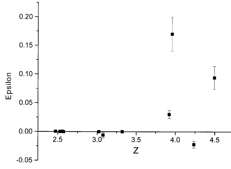
Figure 1: $\epsilon$ for each of the emission and absorption line pairs, against the mean $Z$ value for the QSO.

In conclusion, the statistical tests and experimental data are all consistent with $\epsilon=0$ for $Z\leq 3.3$, but the experimental data support non zero $\epsilon$ values for $Z\geq 4$. High spectral resolution data for $Z\geq 4$ would allow $\epsilon$ in the early universe to be better determined.

Acknowledgments: This research has made use of the SIMBAD database, operated at CDS, Strasbourg, France. We would also like to thank the SIMBAD staff for their assistance, and for providing one of us (DJB) with an account to search their database for high $Z$ QSOs.

References

- [1] See the recent review: ”Early History of Gauge Theories and Kaluza-Klein Theories”, Lochlain O’Raifeartaigh and Norbert Straumann, hep-ph/9810524; Also: Modern Kaluza-Klein Theories, T. Appelquist, A. Chodos and P. G. O. Freund (Eds.), Frontiers in Physics, vol. 65, Addison-Wesley, Reading, MA, 1987.
- [2] Anton Zeilinger and Karl Svozil, Phys. Rev. Lett. 54 (1985) 2553.
- [3] M. Rauch, Annu. Rev. Astron. Astrophys. 36 (1998) 267; C. R. Lynds, Astrophys. J. 164 (1971) L73; W. L. W. Sargent et al., Astrophys. J. Suppl. Ser. 42 (1980) 41.
- [4] J. K. Webb et al., Phys. Rev. Lett. 82 (1999) 884; See also: M. J. Drinkwater et al., Mon. Not. R. Astron. Soc. 295 (1998) 457; S. A. Levshakov, Mon. Not. R. Astron. Soc. 269 (1994) 339.
- [5] Berndt Müller and Andreas Schäfer, Phys. Rev. Lett. 56 (1986) 1215; J. Phys. A19 (1986) 3891.
- [6] David Hochberg and James T. Wheeler, Phys. Rev. D43 (1991) 2617.
- [7] Adam Dobrzycki, Astrophys. J. 457 (1996) 102.
- [8] David Tytler et al., Astron. J. 106 (1993) 426.
- [9] L. J. Storrie-Lombardi et al., Astrophys. J. 468 (1996) 121.
- [10] M. Rugers and C. J. Hogan, Astrophys. J. 459 (1996) L1.
- [11] 100 Statistical Tests, Gopal K. Kanji, Sage Publications, Thousand Oaks, California, 1999.