Moduli as Inflatons in Heterotic M-theory

Abstract:

We consider different cosmological aspects of heterotic M-theory. In particular we look at the dynamical behaviour of the two relevant moduli in the theory, namely the length of the eleventh segment ($\pi\rho$) and the volume of the internal six manifold ($V$) in models where supersymmetry is broken by multiple gaugino condensation. We look at different ways to stabilize these moduli, namely racetrack scenarios with and without non-perturbative corrections to the Kähler potential. The existence of different flat directions in the scalar potential, and the way in which they can be partially lifted, is discussed as well as their possible role in constructing a viable model of inflation. Some other implications such as the status of the moduli problem within these models are also studied.

1 Introduction

The formulation by Hořava and Witten [1] of the field theoretical limit of strongly coupled string theory (or M-theory) as an eleven-dimensional ($d=11$) supergravity (SUGRA) compactified on a manifold with boundaries (explicitly studied in the case of a Calabi–Yau (CY) manifold times the eleventh segment [2]), coupled to $d=10$ supersymmetric (SUSY) Yang–Mills theories, opened up new ways of trying to understand the different problems that we have come across in our attempt to use string theories to obtain a complete picture of the elementary particle world.

In particular we have in this theory two components of the boundary which contain one $E_{8}$ super-Yang–Mills sector each. They communicate through gravitational interactions and one of them is more strongly coupled than the other. Altogether the picture we get is that of two walls (so-called hidden and observable) that interact through gravity, the more strongly coupled being a straightforward candidate to give rise to the condensation of gauginos [3], the fermionic partners of gauge bosons.

Among the different phenomenological achievements of these constructions we find that the experimentally determined unification scale of $10^{16}$ GeV can be reconciled with the effective $d=4$ Planck scale of $10^{18}$ GeV [2, 4], the pattern of soft breaking terms can give gaugino masses of the order of scalar masses [5], and there are candidates for the QCD axion [6] and quintessence [7].

However, and despite all these successes, the two main issues concerning string theories in general remain unsolved, namely those of moduli stabilization and supersymmetry breaking. Whether these two are related or not is still an open question (see, for example, the recent discussion of [8]) but, for the remainder of this paper, we shall assume that they are. More precisely, we shall study the stabilization of the moduli (i.e. the dilaton $S$ and modulus $T$) through gaugino condensation in the hidden wall. These moduli are the superfields whose vacuum expectation values (VEVs) are directly related to two observable quantities, the volume of the CY manifold and the length of the eleventh segment. In order to reproduce the phenomenologically preferred values for the unification scale and coupling constant, those two quantities must be of order $(3\times 10^{16}\;{\rm GeV})^{-6}$ and $(4\times 10^{15}\;{\rm GeV})^{-1}$ respectively.

Therefore, given the scales at which gauginos condense ($\sim 10^{11}$ GeV), we will work directly with the $d=4$ effective theory coming from $d=11$ SUGRA, disregarding an intermediate $d=5$ effective theory in between the Calabi–Yau compactification scale, and that of the eleventh segment [4, 9]. Altogether, we follow the approach of Choi and collaborators [10] by also considering the effect of membrane instantons that result in a non-perturbative contribution to the Kähler potential.

Once we have defined a model within which we achieve SUSY breaking at the right scale, we can proceed to study the cosmological behaviour of these moduli fields. Inflation due to F-terms in the scalar potential has always been considered a generic problem of SUGRA theories essentially due to the absence of flat-enough directions. However several attempts have been made to build string-inspired inflationary potentials, having either the moduli [11, 12] or matter fields [13] as inflatons.

In our case we start our analysis of the cosmological viability of our model by noting very general features of the scalar potential defined by multiple gaugino condensation (or racetrack) models in the context of M-theory, namely the existence of flat and almost flat directions for two and more condensates, respectively. As mentioned before, flat directions are always of interest in cosmology, and indeed we study the capability of these models to drive inflation and, in particular, of the moduli fields to become suitable inflatons.

Together with inflation, the other main cosmological issue about string-derived models is the so-called moduli problem [14]. It turns out that, in general, moduli are very weakly interacting particles with VEVs of the order of the Planck scale and masses of the order of the electroweak scale, which makes them very dangerous relics from the point of view of the evolution of the Universe. In the final part of this paper we consider this problem, calculating their masses and pointing out which of them would be in a cosmologically dangerous range.

Therefore the plan of this paper is as follows. In section 2 we study the stabilization of the moduli through gaugino condensation in the hidden wall. First of all we point out a few general features of scalar potentials due to multiple gaugino condensation, which are independent of the form of the Kähler potential used, namely the presence of flat and almost flat directions. We shall also see that, in order to achieve the desired VEVs for the moduli, with SUSY broken at the right scale (given by a gravitino mass, $m_{3/2}$, of about $1$ TeV) we can either invoke pure multiple gaugino condensation (also denoted as the racetrack mechanism) or combine it with some non-perturbative corrections to the Kähler potential, which will ensure the cancellation of the cosmological constant at the minimum (the so-called Kähler stabilization). In order to illustrate these results we present a detailed calculation with a particular ansatz for $K_{\rm np}$.

In section 3 we consider the cosmological evolution of these fields. The presence of the flat directions demonstrated in section 2 opens up the possibility of achieving inflation with some combination of the moduli fields as the inflaton. We study the behaviour of the different candidates for inflatons, and we select the ones that give an acceptable pattern of inflation. Continuing with cosmological issues, in section 4 we study the moduli problem of these models. We calculate the moduli masses, and point out possible problems of those associated with the flat directions, as well as possible solutions. We conclude in section 5.

2 Stabilization of the moduli

As mentioned in the introduction, we want to study various phenomenological features of compactified heterotic M-theory constructions where SUSY is broken by gaugino condensation. The two dynamical quantities we need to stabilize are $\rho$, the length of the eleventh segment, and $V$, the volume of the internal manifold. Those are related to the chiral superfields $S$, $T$ through

$${\rm Re}\;S = (4\pi)^{-2/3}\kappa^{-4/3}V\;\;,$$

$${\rm Re}\;T = \left(4\pi\sum_{IJK}C_{IJK}/6\right)^{-1/3}\kappa^{-2/3}\pi\rho V^{1/3}\;\;,$$

where $\kappa^{2}$ is the $d=11$ gravitational coupling, and $C_{IJK}$ are the CY intersection numbers.

From now on we shall follow the notation of Ref. [10] and define the phenomenologically preferred values:

$$\langle{\rm Re}\;S\rangle = \langle S_{\rm R}\rangle=O(\alpha_{\rm GUT}^{-1})\;\;,$$

$$\langle{\rm Re}\;T\rangle = \langle T_{\rm R}\rangle=O(\alpha_{\rm GUT}^{-1})\;\;,$$

in units of the $d=4$ Planck mass, $M_{\rm P}$ ($=\kappa^{-1}\sqrt{\pi\rho V}$). In order to study the stabilization of these fields we need to calculate the scalar potential, which is made out of two functions, the superpotential $W$ and the Kähler potential $K$. The latter can be divided into two pieces, a perturbative one ($K_{\rm p}$), which admits an expansion in powers of $1/S_{\rm R}$, $1/T_{\rm R}$ (and can be determined in different M-theory limits [15, 16]), and $K_{\rm np}$, which contains all non-perturbative effects. Therefore we have

$$K=K_{\rm p}+K_{\rm np}=K_{0}+\delta K_{\rm p}+K_{\rm np}\;\;,$$ (3)

where

$$K_{0}=-\log(S+\bar{S})-3\log(T+\bar{T})$$ (4)

and $\delta K_{\rm p}$ stands for higher-order corrections to the perturbative expansion. In this context, $K_{\rm np}$ stands for the M-theory version of stringy non-perturbative effects [17], which are given by different types of instantons wrapping several cycles of the CY. These were computed first in [18] for the case of type IIA M-theory and the discussion was extended in [10] to heterotic M-theory. Out of the three different types of instantons we can have, membrane instantons wrapping the CY 3-cycle ($I_{1}\sim b\sqrt{S_{\rm R}}$), membrane instantons wrapping the CY 2-cycle ($I_{2}\sim 2\pi T$), and five-brane instantons wrapping the entire CY volume ($I_{3}\sim 2\pi S$), only the first ones are going to give a significant contribution to $K_{\rm np}$, which goes as $e^{-I_{1}}$.

As for the superpotential, we shall consider multiple gaugino condensation

$$W=\sum_{a}C_{a}e^{-\alpha_{a}f_{a}}+O(e^{-2\pi S},e^{-2\pi T})\;\;,$$ (5)

where $a$ labels the corresponding hidden gauge group $G_{a}$, $\alpha_{a}$ are the corresponding one-loop beta function coefficients ($\alpha_{a}=24\pi^{2}/(3N_{a}-M_{a})$ for SU($N_{a}$) with $M_{a}$ pairs of matter fields transforming as $N_{a}$, $\bar{N}_{a}$), the $C_{a}$ coefficients depend on $N_{a}$ and $M_{a}$, and $f_{a}$ are the gauge kinetic functions, defined as

$$f_{a}=\frac{1}{4\pi}\left(S-\frac{n_{a}}{2}T\right)+O(e^{-2\pi S},e^{-2\pi T})\;\;.$$ (6)

Their exact form is currently known for smooth CY compactifications [6, 19, 16], even in the presence of five-branes [20], and they have been studied for orbifold compactifications in [21].

Finally the scalar potential is given by

$$V=e^{K}\left\{\left|W_{S}+K_{S}W\right|^{2}(K_{S\bar{S}})^{-1}+\left|W_{T}+K_{T}W\right|^{2}(K_{T\bar{T}})^{-1}-3\left|W\right|^{2}\right\}\;\;,$$ (7)

where the subindices indicate derivatives of $W$ and $K$ with respect to the different fields.

The next step will be to minimize this potential, and study the possibility of finding minima with zero cosmological constant, i.e. we want the conditions $\partial V/\partial S=\partial V/\partial T=0$ (together with $V|_{\rm min}=0$ whenever it is possible) to be fulfilled for values of $S_{\rm R}$, $T_{\rm R}$ given by Eq. (LABEL:app). Before getting into the numerical details of our calculation, let us note a very distinctive feature of these kinds of potentials, namely the possibility of having flat directions along the imaginary components of $S$ and $T$. This fact was already noted in [10] for the case of two condensates, and is generalized here, independently of the form of $K$. It only relies on the form of the gauge kinetic functions $f_{a}$.

2.1 Imaginary directions

We will start our analysis by looking for minima in the imaginary directions of the moduli fields, $S_{\rm I}=\mathrm{Im}\;S$ and $T_{\rm I}=\mathrm{Im}\;T$. In the case of one single condensate, where the superpotential is $W=Ce^{-\alpha(S-nT/2)}$, the scalar potential of Eq. (7) is totally independent of the phase of the superpotential. Therefore both $S_{\rm I}$ and $T_{\rm I}$ will be flat directions of the scalar potential.

Let us now consider the case of a two-condensate racetrack model, where the superpotential of Eq. (5) is given by

$$W=W_{1}+W_{2}\;\;,$$ (8)

with $W_{1}=C_{1}e^{-\alpha_{1}(S-n_{1}T/2)}$ and $W_{2}=C_{2}e^{-\alpha_{2}(S-n_{2}T/2)}$. Intuitively, one expects that one of the phases can still be factored out from the scalar potential, as in the one-condensate case, leaving a flat direction in the potential. We can easily check this result by calculating the derivatives of the scalar potential with respect to the imaginary fields. From Eq. (7), we obtain the derivative with respect to $S_{\rm I}$:

$$\frac{\partial V}{\partial S_{\rm I}}=-2\ \mathrm{Im}\left({\frac{\partial V}{\partial S}}\right)=-\frac{\alpha_{2}-\alpha_{1}}{2\pi}\;e^{K}A\ \mathrm{Im}(\bar{W_{1}}W_{2})\;\;,$$ (9)

where

$$A=3-\frac{(K_{\bar{S}}-\alpha_{1}/4\pi)(K_{S}-\alpha_{2}/4\pi)}{K_{S\bar{S}}}-\frac{(K_{\bar{T}}+n_{1}\alpha_{1}/8\pi)(K_{T}+n_{2}\alpha_{2}/8\pi)}{K_{T\bar{T}}}$$ (10)

is a quantity independent of $S_{\rm I}$ and $T_{\rm I}$. Similarly, the derivative with respect to $T_{\rm I}$ is

$$\frac{\partial V}{\partial T_{\rm I}}=-2\ \mathrm{Im}\left({\frac{\partial V}{\partial T}}\right)=\frac{n_{2}\alpha_{2}-n_{1}\alpha_{1}}{4\pi}e^{K}A\ \mathrm{Im}(\bar{W_{1}}W_{2})\;\;,$$ (11)

with $A$ still given by Eq. (10). A sufficient condition for a stationary point is then

$$\mathrm{Im}(\bar{W_{1}}W_{2})=0\;\;,$$ (12)

which yields

$$\Phi^{-}_{\rm i}\equiv S_{\rm I}-\frac{n_{1}\alpha_{1}-n_{2}\alpha_{2}}{2(\alpha_{1}-\alpha_{2})}T_{\rm I}=\frac{4\pi^{2}k}{\alpha_{1}-\alpha_{2}}\;\;,$$ (13)

where we have defined a new field $\Phi^{-}_{\rm i}$ and $k$ is an integer. It is easy to check that $k$ even corresponds to a maximum and $k$ odd to a minimum. More importantly, this relation does not fix both $S_{\rm I}$ and $T_{\rm I}$, a good indication that there is a flat direction in the potential. Indeed, the direction orthogonal to $\Phi^{-}_{\rm i}$,

$$\Phi^{+}_{\rm i}\equiv\frac{n_{1}\alpha_{1}-n_{2}\alpha_{2}}{2(\alpha_{1}-\alpha_{2})}S_{\rm I}+T_{\rm I}\;\;,$$ (14)

is a flat direction of the potential, for which $\frac{\partial V}{\partial\Phi^{+}_{\rm i}}=0$ for all values of the fields.

So what happens if we have more than two condensates? Naively we would expect that, even though one of the phases can be factored out from the scalar potential as before, the remaining ones should be able to stabilize both directions in the imaginary fields. The superpotential is given by the general formula of Eq. (5), and the imaginary derivatives will be

$$\frac{\partial V}{\partial S_{\rm I}}=-\frac{e^{K}}{2\pi}\sum_{i<j}\left[A_{ij}(\alpha_{j}-\alpha_{i})\;\mathrm{Im}(\bar{W_{i}}W_{j})\right]\;,$$ (15)

and

$$\frac{\partial V}{\partial T_{\rm I}}=\frac{e^{K}}{4\pi}\sum_{i<j}\left[A_{ij}(n_{j}\alpha_{j}-n_{i}\alpha_{i})\;\mathrm{Im}(\bar{W_{i}}W_{j})\right]\;\;,$$ (16)

where

$$A_{ij}=3-\frac{(K_{S}-\alpha_{i}/4\pi)(K_{\bar{S}}-\alpha_{j}/4\pi)}{K_{S\bar{S}}}-\frac{(K_{T}+n_{i}\alpha_{i}/8\pi)(K_{\bar{T}}+n_{j}\alpha_{j}/8\pi)}{K_{T\bar{T}}}$$ (17)

are again independent of $S_{\rm I}$ and $T_{\rm I}$.

The condition for the existence of a flat direction, $a\frac{\partial V}{\partial S_{\rm I}}+b\frac{\partial V}{\partial T_{\rm I}}=0$ for some $a$ and $b$ independent of $S_{\rm I}$ and $T_{\rm I}$, becomes

$$0=\sum_{i<j}\left[A_{ij}\left(a(\alpha_{j}-\alpha_{i})+\frac{b}{2}(n_{j}\alpha_{j}-n_{i}\alpha_{i})\right)\;\mathrm{Im}(\bar{W_{i}}W_{j})\right]\;.$$ (18)

In the case of a single gauge kinetic function parameter, $n=n_{i}=n_{j}$ for all $(i,j)$, and $a=-nb/2$ is then an obvious solution. In other words, if all the $n_{i}$ are the same, there is always a flat direction in the imaginary fields, for any number of condensates in the hidden sector. On the other hand, if one of the $n_{i}$ differs from the others, it is impossible to find a solution to Eq. (18) holding for all $S_{\rm I}$ and $T_{\rm I}$, so all the flat directions in the imaginary fields become lifted.

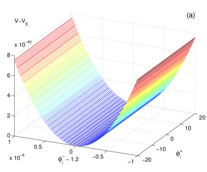
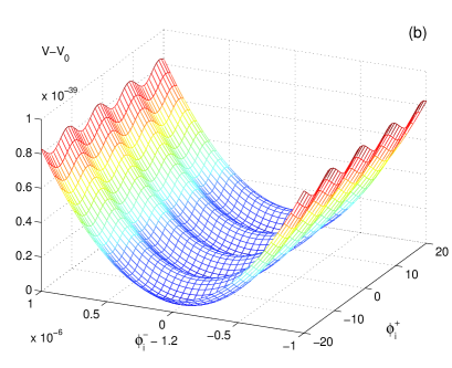
Figure 1: 3-d plot of the scalar potential $V$ as a function of $\Phi^{-}_{\rm i}=S_{\rm I}-T_{\rm I}/2$ and $\Phi^{+}_{\rm i}=S_{\rm I}/2+T_{\rm I}$ (in $M_{\rm P}$ units) for the case of (a) two condensates with $N_{1}=3$, $M_{1}=0$, $N_{2}=4$, $M_{2}=8$ and gauge kinetic function parameters $n_{1}=n_{2}=1$ and (b) three condensates, consisting of the previous two plus a third one given by $N_{3}=2$, $M_{3}=0$ and $n_{3}=0.5$. We can see that the flat direction of (a) is lifted in (b) by the presence of the third condensate. In both examples we have set the $K_{\rm np}$ parameters to $D=0.13$ and $B=120$, and fixed the real values of the fields to their minima $S_{\rm R}\sim 19$ and $T_{\rm R}\sim 15.9$ (see section 2.2). $V_{0}$ is the value of the potential at the minimum.

As an illustration of this vacuum structure for these models, we have plotted in Fig. 1 the scalar potential versus the orthogonal combinations of the imaginary fields, for an example of two and three condensates. We can clearly see in the second picture how the flat direction is lifted by the presence of the third condensate with a different gauge kinetic function parameter. We will explore the cosmological interest of these features in section 3.

2.2 Real directions

We will look now at the minimization of the potential, Eq. (7), along the real components, $S_{\rm R}$ and $T_{\rm R}$. In particular we are going to analyse two different situations: Kähler stabilization and pure racetrack models.

Let us start with the pure racetrack case, that is, a Kähler potential given only by its perturbative piece, $K=K_{0}$ in Eq. (3). The real directions are in a way similar to the imaginary directions, in the sense that the interplay between two condensates, through the superpotential contributions to the scalar potential of Eq. (7), will be able to fix the combination $\Phi_{\rm r}^{-}=S_{\rm R}-\frac{n_{1}\alpha_{1}-n_{2}\alpha_{2}}{2(\alpha_{1}-\alpha_{2})}T_{\rm R}$, whereas the orthogonal combination $\Phi^{+}_{\rm r}=\frac{n_{1}\alpha_{1}-n_{2}\alpha_{2}}{2(\alpha_{1}-\alpha_{2})}S_{\rm R}+T_{\rm R}$ will factor out from the superpotential contributions. However, contrary to the imaginary case, this direction will not be flat because of extra terms arising from the Kähler potential contributions to Eq. (7). We have checked that these Kähler terms will always yield a runaway potential, provided all the gauge kinetic parameters $n_{i}$ are the same. This is true for any number of condensates in the hidden sector. So if we want to find a minimum for the real fields, we need to introduce different $n_{i}$ or non-perturbative corrections to the Kähler potential.

To illustrate the first case, we have found a few examples where the real directions are indeed fixed with only two condensates having different gauge kinetic function parameters. These are presented in Table 1. The results are similar to the usual ones obtained in the weakly coupled case [22], in particular the potential energy at the minimum turns out to be always negative.

$N_{1}$	$M_{1}$	$n_{1}$	$N_{2}$	$M_{2}$	$n_{2}$	$S_{\rm R}$	$T_{\rm R}$	$m_{3/2}(\mathrm{GeV})$
3	8	1.00	2	0	1.06	17.6	20.7	1090
3	7	1.40	2	0	1.45	22.0	20.3	120
5	7	1.00	4	0	1.04	26.9	23.7	74

Table 1: Some examples of minima in a pure racetrack scenario.

We now turn to the second possibility, including non-perturbative corrections to the Kähler potential. In order to do that we choose a particular ansatz for $K_{\rm np}$ [23], which gives a zero cosmological constant at the minimum of the potential,

$$K_{\rm np}=\frac{D}{B\sqrt{S_{\rm R}}}\log\left(1+e^{-B(\sqrt{S_{\rm R}}-\sqrt{S_{0}})}\right)\;\;,$$ (19)

where we fix $S_{0}=19$, and the different vacua, for a given $W$, are functions of pairs of values ($D$, $B$).

Apart from having a different ansatz for $K_{\rm np}$, the rest of the vacuum structure is totally analogous to that found in [10]. The case of one condensate does not result in any minima with the right order of magnitude for $S_{\rm R}$, $T_{\rm R}$ (see Eq. (LABEL:app)), whereas two or more condensates yield the desired results, with the $K_{\rm np}$ correction stabilizing the previously runaway direction $\Phi_{\rm r}^{+}$. To obtain reasonable values for $S_{\rm R}$ and $T_{\rm R}$, we require the presence of hidden matter fields, transforming under the hidden gauge groups, in a way similar to what happened in weakly coupled heterotic string theories [22].

We will now consider the cosmological possibilities of both these types of solutions in turn.

3 Cosmological evolution

In order to study the cosmological evolution of the moduli fields we have to solve their equations of motion in an expanding Universe. These are given by

$$K_{S\bar{S}}(\ddot{S}+3H\dot{S})+K_{SS\bar{S}}\dot{S}^{2}+\frac{\partial{V}}{\partial{\bar{S}}} = 0$$

$$K_{T\bar{T}}(\ddot{T}+3H\dot{T})+K_{TT\bar{T}}\dot{T}^{2}+\frac{\partial{V}}{\partial{\bar{T}}} = 0\;\;,$$

with $H$, the Hubble constant, given by

$$H^{2}=\frac{1}{3}K_{S\bar{S}}\dot{S}\dot{\bar{S}}+\frac{1}{3}K_{T\bar{T}}\dot{T}\dot{\bar{T}}+\frac{V}{3}\;.$$ (21)

As we can see, the presence of non-canonical kinetic terms for $S$ and $T$ already imposes a few modifications in the above system, with respect to the usual canonically normalized fields. We will consider in turn the cases of two and three condensates.

Two condensates

Summarizing what was found in the previous section, we have four possible directions of the scalar potential, which are functions of the two complex moduli fields $S$ and $T$. Those corresponding to the combinations $\Phi^{-}_{\rm r,i}$ are, as we said before, fixed by the interplay between the two condensates, much as was done in the weakly coupled heterotic string [22]. Therefore, along these two directions, the behaviour from the cosmological point of view is very similar to the one in the stringy case, which was studied in Ref. [24], only that now the gauge kinetic functions are given by Eq. (6) rather than just $4\pi f_{a}=k_{a}S$ ($k_{a}$ is the Kac–Moody level of the corresponding gauge group). The conclusion of that study was that, along the $S$ direction (which is $\Phi^{-}$ now) the potential is too steep to the left of the minimum to guarantee that the field will settle down in the latter instead of rolling past. Moreover its kinetic energy is too big to drive inflation during its evolution.

We face here exactly the same situation and therefore conclude that, along the above-mentioned directions, no new features arise. However it is worth mentioning that, in the presence of a dominating background, this combination of fields could reach a scaling regime just like $S$ in the heterotic string case [25]. The effects of such background in these M-theory models will be studied elsewhere [26].

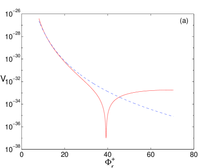
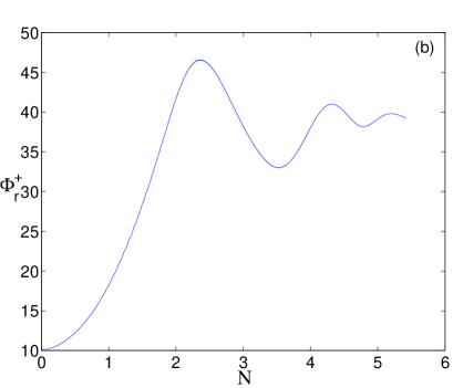
Figure 2: (a) Solid: $V$ as a function of $\Phi_{\rm r}^{+}$ (in $M_{\rm P}$ units) along the valley defined by $\Phi^{-}_{\rm r}=11.07$ for the same example as in Fig. 1a. Dashed: a simple approximation to $V$ given by $Q/(\Phi^{+}_{\rm r})^{9}$; (b) evolution of $\Phi^{+}_{\rm r}$ as a function of $N$ (the number of e-folds) along the same valley as before, but with $K_{np}$ parameters $B=3$ and $D=13.9924$.

Let us now turn to the analysis of the other two remaining directions, namely $\Phi^{+}_{\rm r,i}$. As mentioned before, $\Phi^{+}_{\rm i}$ is a totally flat direction in the case of two condensates, and therefore no evolution is expected. At this stage we could consider the effect of including the higher-order corrections indicated in Eqs. (5) and (6), given that they would introduce terms depending on $S_{\rm I}$ and $T_{\rm I}$. However, when we took these terms into account, we found that the numerical effect is minute, and that no significant differences with respect to the totally flat case can be seen. Nevertheless these corrections can give rise to very interesting potentials concerning the axion mechanism to solve the strong CP problem [6] or quintessence [7]. Neither is it worth considering higher order corrections to the Kähler potential, such as those parametrized by $\delta K_{\rm p}$ in Eq. (3), given that this function carries no dependence on the imaginary parts of either $S$ or $T$.

We are then left with the evolution along $\Phi^{+}_{\rm r}$. This is, a priori, the most promising direction along which to study the evolution of the fields, given that, as mentioned in section 2.2, this field only gets contributions to its scalar potential from the Kähler potential. That is, instead of having an exponential potential like $\Phi_{\rm r}^{-}$, it has a power-law type one. This is true for both the pure racetrack models, where $K_{\rm np}=0$, and the Kähler stabilization models. An example of the evolution of the $\Phi^{+}_{\rm r}$ for the latter models is shown in Fig. 2 for the same two condensing groups as in Fig. 1a, but with $K_{\rm np}$ defined by $B=3$, $D\sim 14$, this time. In this example the direction shown is the orthogonal to that defined by $\Phi^{-}_{\rm r}\sim 11.07$, and the imaginary fields were fixed to their minimum values. In Fig. 2a we have plotted the scalar potential as a function of $\Phi_{\rm r}^{+}$, as well as a quite accurate fit to its slope given by $Q/(\Phi_{\rm r}^{+})^{9}$, with $Q\sim 3.5\times 10^{-19}$. Concerning the cosmological behaviour, we have evolved both $\Phi_{\rm r}^{+}$ and $\Phi^{-}_{\rm r}$ simultaneously, in order to take into account the small oscillations that the latter has around its central value, defining a ‘valley’ in the potential as both fields evolve towards the minimum. As we see in Fig. 2b, a maximum of $\sim 5$ e-folds of evolution can be obtained before the field reaches its minimum (defined by $S_{\rm R}\sim 24.5$, $T_{\rm R}\sim 27$, i.e. $\Phi_{\rm r}^{+}=39.25$) and oscillates around it. Even though this is not a very promising candidate for an inflaton, it is interesting to note the fact that the field does stay at its minimum for a big fraction of initial conditions within this valley.

In fact, these kinds of inflationary models (defined by inverse power-law potentials) are denoted in the literature as ‘intermediate inflation’ [27], and the reason why, in this case, the inflationary period does not last for long enough is that neither $S$ nor $T$ have canonical kinetic terms. With non-minimal kinetic terms the evolution is considerably faster than that of a typical intermediate inflation model. Note that this is also true for the pure racetrack models.

Three condensates

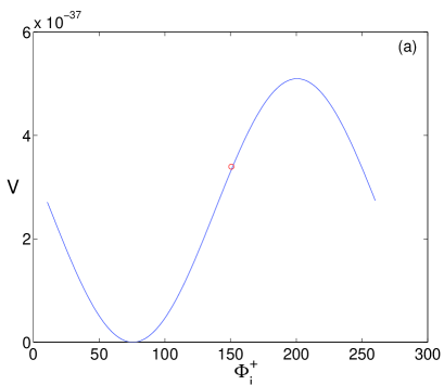
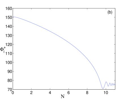
Figure 3: (a) Plot of the potential $V$ as a function of $\Phi^{+}_{\rm i}$ (in $M_{\rm P}$ units) along the bottom of the valley defined by $\Phi^{-}_{\rm i}={\rm constant}$, for the same example as in Fig. 1b, with $n_{3}=0.98$; (b) evolution of $\Phi^{+}_{\rm i}$ as a function of $N$ (the number of e-folds) along the same valley as before and initial conditions given by the circle shown in (a).

As we saw in section 2.1, with three condensates we now have the enticing possibility of lifting the flat direction in the imaginary fields $\Phi^{+}_{\rm i}$ with a sizeable effect. We will then be interested in the evolution of the field along this previously flat direction.

In order to illustrate the lifting of the flat direction, let us assume from now on that we have a perfectly well defined minimum with two condensates, i.e. we define $W_{0}$, given by Eq. (8), as our starting superpotential. Either by Kähler stabilization (with $n_{1}=n_{2}$) or pure racetrack (in which $n_{1}\neq n_{2}$ is required), the corresponding scalar potential provides us with minima for $\Phi_{\rm i}^{-}$ (given by Eq. (13)) and $\Phi_{\rm r}^{\pm}$ (as explained in section 2.2), whereas $\Phi_{\rm i}^{+}$, as defined in Eq. (14), is the flat direction.

Now let us add a third condensate to this system, in such a way that the position of the already determined minimum is not substantially affected. This will happen if the $\beta$ function coefficient of this third condensate is considerably smaller than that of the other two, so that $\alpha_{3}=24\pi^{2}/(3N_{3}-M_{3})\ll\alpha_{1},\alpha_{2}$. This third condensate, with gauge kinetic function given by $4\pi f_{3}=S-n_{3}T/2$, will contribute to the scalar potential through a term in the superpotential given by $C_{3}e^{-\alpha_{3}f_{3}}$. This will generate an extra piece in the scalar potential along the formerly flat direction given by

$$V_{\rm new}\approx V_{13}(1+\cos(\varphi_{13}))\;\;,$$ (22)

where

$$V_{13} = 2e^{K}C_{3}e^{-\alpha_{3}(S_{\rm R}-n_{3}T_{\rm R}/2)}\left[\frac{1}{K_{S\bar{S}}}(K_{S}W_{0}|_{\rm min}+{W_{0S}|_{\rm min}})\left(K_{S}-\frac{\alpha_{3}}{4\pi}\right)\right.$$ (23)

$$+ \left.\frac{1}{K_{T\bar{T}}}(K_{T}W_{0}|_{\rm min}+{W_{0T}|_{\rm min}})\left(K_{T}+\frac{n_{3}\alpha_{3}}{8\pi}\right)-3W_{0}|_{\rm min}\right]\;\;,$$

with $W_{0}|_{\rm min}=C_{1}e^{-\alpha_{1}(S_{\rm R}-n_{1}T_{\rm R}/2)}-C_{2}e^{-\alpha_{2}(S_{\rm R}-n_{2}T_{\rm R}/2)}$, $\Phi^{-}_{\rm i}$ is fixed at the value for which the two first condensates have opposite phases and

$$\varphi_{13}=\frac{1}{4\pi}\left[(\alpha_{3}-\alpha_{1})S_{\rm I}-(n_{3}\alpha_{3}-n_{1}\alpha_{1})\frac{T_{\rm I}}{2}\right]\;\;.$$ (24)

In Fig. 3a we have plotted the potential $V_{\rm new}$ versus $\Phi_{\rm i}^{+}$ for the same example as in Fig. 1b, this time with $n_{3}=0.98$. The shape of this potential follows, as expected, Eq. (22). Concerning the cosmological evolution of the now non-flat field $\Phi_{\rm i}^{+}$, this is shown in Fig. 3b for the same example as given in Fig. 3a with the initial condition there represented by a circle. This corresponds to starting the evolution with a potential energy equal to $60\%$ of the maximum of the cosine potential, and it lasts for less than 10 e-folds. The model corresponds to the so-called natural inflation [28].

Encouraged by these results, we will now try to find out under which conditions we could achieve more e-folds of inflation. It turns out that the closer $n_{3}$ is to $n_{1}$ the flatter the potential is along $\Phi_{\rm i}^{+}$. In fact for $n_{3}=n_{1}$ we should recover the flat direction that the two first condensates had defined. Therefore imposing $n_{3}\sim n_{1}$ should give us a potential as flat as we wish. This is shown in Fig. 4a, where we evolve the field $\Phi_{\rm i}^{+}$ for the same example as before, only that this time we set $n_{3}=0.995$. As we can see, we can easily obtain more than 60 e-folds of inflation.

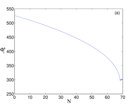
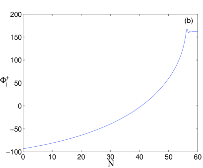
Figure 4: Evolution of $\Phi^{+}_{\rm i}$ (in $M_{\rm P}$ units) as a function of $N$ (the number of e-folds) along the bottom of the valley defined by $\Phi^{-}_{\rm i}={\rm constant}$, for: (a) the same Kähler stabilization model as in Fig. 3, with $n_{3}=0.995$ and similar initial conditions; (b) a pure racetrack model given by $N_{1}=5$, $M_{1}=7$, $N_{2}=4$, $M_{2}=0$, $N_{3}=3$, $M_{3}=2$, $n_{1}=n_{3}=1$, $n_{2}=1.04$ and initial conditions near the maximum of its potential.

The same is true for the pure racetrack case, which is shown in Fig. 4b. The example we have chosen is the last one of Table 1, to which we have added a third condensate given by $N_{3}=3$, $M_{3}=2$, $n_{3}=1$. In general these models suffer from the problem that the phenomenologically acceptable vacua correspond to potentials that are not flat enough. The closer we try to bring all three $n_{i}$ parameters to each other in order to create a smaller slope, the smaller the gravitino mass becomes. One of the best examples we have is the one shown here, where we obtain more than 50 e-folds of inflation, but at the price of starting the evolution almost at the maximum of the potential. From this model-building point of view, the models with Kähler stabilization are somehow favoured. Also note that, in order to perform the evolution of the fields in this pure racetrack models, we have had to cancel the negative vacuum energy by adding a constant to the scalar potential. This is equivalent to assuming that some unknown mechanism is responsible for the cancellation of the cosmological constant.

Finally let us add a few comments concerning the scale of these types of inflation. The energy scale of the potential is similar to the scale of the gaugino condensates, that is around $10^{11}\;\mathrm{GeV}$. As the model stands, a simple single-field slow-roll type of inflation, this would undoubtedly be too low to explain the cosmic microwave background anisotropy and large scale structure. This flat direction could eventually be incorporated in a hybrid inflation type of scenario [12, 29], where the density fluctuations can be generated with this sort of energy scale. This, however, would go far beyond the scope of this paper. Alternatively, this flat direction could be used to implement a scenario of weak inflation [30], of the type used to solve the moduli problem.

4 Moduli problem

We are going to conclude this analysis of the cosmological behaviour of the moduli in heterotic M-theory by revisiting the moduli problem from that point of view. Moduli are, in the weakly coupled heterotic string, very dangerous relics from the cosmological point of view, given that they have large vacuum expectation values (of the order of $M_{\rm P}$) and light masses (of the order of the gravitino mass, $m_{3/2}$). The potential cosmological problems of light, weakly interacting particles had already been pointed out in the context of supergravity [31] and superstrings [32], but were explicitly addressed for moduli in Refs. [14]. Altogether, if moduli decay they should do so before nucleosynthesis, in order not to spoil its predictions for the abundance of light elements. This imposes a lower bound of their masses given by

$$m_{S,T}\leq O(10\;{\rm TeV})\;.$$ (25)

On the other hand, if these particles do not decay they should not overclose the Universe today. This imposes an upper bound on their masses, in the absence of inflation, given by $m_{S,T}\geq 1\;{\rm keV}$. This bound applies both to the moduli and their fermionic partners, the modulini; in principle, it could be avoided with a period of inflation at a scale low enough to dilute them and avoid their regeneration in large amounts.

However, for the scalars there is an additional problem, which is that, at the end of inflation, these particles will probably be shifted from their zero temperature minima. It has been estimated that during their evolution towards their true minima, these fields will oscillate and their energy density will increase substantially. For stable moduli this imposes an upper bound on their masses given by

$$\frac{m_{\phi}}{100\;{\rm GeV}}\leq\left(10^{10}\frac{\phi_{\rm in}}{M_{\rm P}}\right)^{-4}\;\;,$$ (26)

where $\phi=S,T$ and $\phi_{\rm in}$ is the value of the shift at the end of inflation, which is typically of order $M_{\rm P}$ (actually, in the examples presented above it is of order $100\;M_{\rm P}$, see Figs. 3 and 4). From here we get extremely tight upper bounds for the masses of the stable moduli, of the order of $10^{-24}\;{\rm eV}$.

Several mechanisms have been proposed to cure this problem, the most promising of which is to invoke a period of thermal inflation [33] just before nucleosynthesis in order to dilute these unwanted relics. In particular, it has been shown in Ref. [34] that it can solve the overclosure problem of the stable moduli if their masses are in the range of $10\;{\rm eV}$ to $10^{4}\;{\rm GeV}$. This is particularly important for the forthcoming discussion.

Let us then turn to the issue of moduli masses in these heterotic M-theory models we have just analysed. We have calculated and diagonalized the mass matrix for the four real components, namely $S_{\rm R}$, $T_{\rm R}$, $S_{\rm I}$ and $T_{\rm I}$, both for the cases of Kähler stabilization and pure racetrack models. In both scenarios the results are rather similar and the eigenvectors do correspond to the directions $\Phi^{+}_{\rm r,i}$, $\Phi^{-}_{\rm r,i}$ defined in previous sections, which shows that our choice corresponds to the physical directions. To illustrate this, we present two examples where we have calculated the moduli masses.

• $K_{\rm np}\neq 0$. The example chosen is ${\rm SU}(3)_{M=0}\times{\rm SU}(4)_{M=8}\times{\rm SU}(2)_{M=0}$, with $n_{1}=n_{2}=1$

  $$m_{\Phi_{\rm r}^{-}},m_{\Phi_{\rm i}^{-}} \sim 3\times 10^{3}\;m_{3/2}$$

  $$m_{\Phi_{\rm r}^{+}} \sim 40\;m_{3/2}$$ (27)

  $n_{3}=0.98$	$\rightarrow$	$m_{\Phi_{\rm i}^{+}}$	$\sim$	$10^{-3}\;m_{3/2}$
  $n_{3}=0.995$	$\rightarrow$	$m_{\Phi_{\rm i}^{+}}$	$\sim$	$10^{-4}\;m_{3/2}$

• $K_{\rm np}=0$. The example chosen is ${\rm SU}(3)_{M=2}\times{\rm SU}(5)_{M=7}\times{\rm SU}(4)_{M=0}$, with $n_{1}=n_{2}=1$

  $$m_{\Phi_{\rm r}^{-}},m_{\Phi_{\rm i}^{-}} \sim 10^{4}\;m_{3/2}$$

  $$m_{\Phi_{\rm r}^{+}} \sim 2\;m_{3/2}$$ (28)

  $n_{3}=1.04$	$\rightarrow$	$m_{\Phi_{\rm i}^{+}}$	$\sim$	$7\times 10^{-4}\;m_{3/2}$
  $n_{3}=1.05$	$\rightarrow$	$m_{\Phi_{\rm i}^{+}}$	$\sim$	$6\times 10^{-4}\;m_{3/2}\;\;.$

As we can see, the combination of moduli associated with the steepest directions, $\Phi^{-}_{\rm r,i}$, are heavy enough to fulfil the lower bound given by Eq. (25), and it is the other two combinations of moduli, $\Phi^{+}_{\rm r,i}$, which are in trouble with the existing bounds. In particular, the mass associated with the almost flat direction $\Phi^{+}_{\rm i}$ is, as expected, smaller as $n_{3}$ is closer to either $n_{1}$ or $n_{2}$; it should be exactly zero in the limit in which it becomes equal to one of them, i.e. when we recover the flat direction typical of the two-condensate case. Such a light modulus is not likely to decay at all, and therefore the bound given by Eq. (26) should be applicable to it. A period of thermal inflation would then be desirable for these two lighter moduli not to become unwanted relics.

We have also analysed the possible reasons for this pattern of masses to be so different from that of the weakly coupled heterotic models, in which all moduli masses were of the order of $m_{3/2}$. Apart from the different curvatures of the potential along the different directions, which are now different and explain the existing hierarchy between the different combinations of moduli, the difference in magnitude can be attributed to the difference of the magnitude of the Kähler metric at the minimum of the potential. As we know, and as was pointed out in the previous section, the moduli $S$ and $T$ are not canonically normalized particles as the kinetic terms of their Lagrangian are given by

$${\cal L}_{\rm kin}=K_{S\bar{S}}D_{\mu}SD^{\mu}\bar{S}+K_{T\bar{T}}D_{\mu}TD^{\mu}\bar{T}\;\;.$$ (29)

In order to obtain the physical masses, we must transform the fields into canonically normalized ones, and the transformation induces inverse powers of $K_{S\bar{S}}$, $K_{T\bar{T}}$ in the mass matrix. So far, this was also the case in the weakly coupled heterotic string, the difference being the different magnitudes of these derivatives in the two theories. Before, the expected values for the moduli at the minimum were or order 1, and therefore these normalization factors would also have the same size (note that, for example, for $K_{0}$ we have $K_{S\bar{S}}\sim 1/(2S_{\rm R})^{2}$, $K_{T\bar{T}}\sim 3/(2T_{\rm R})^{2}$). However, in heterotic M-theory we look for minima of the potential corresponding to $S$, $T$ of order 20 (always in $M_{\rm P}$ units), which implies that the normalized masses are suppressed by factors of $10^{-4}$-$10^{-3}$, and therefore enhanced in absolute value.

5 Conclusions

In this paper we have studied the dynamics of the two typical M-theory moduli, namely the volume of the 6-dimensional manifold $V$ and the orbifold that parametrizes the $11^{\rm th}$ segment $\pi\rho$ in terms of the dilaton $S$ and an overall modulus $T$. Assuming gaugino condensation in the hidden wall as the source of SUSY breaking, we studied the resulting scalar potential for different numbers of condensates in the case of the so-called Kähler stabilization (where $K=K_{0}+K_{\rm np}$) and pure racetrack models ($K=K_{0}$). In both cases a determinant feature of the vacuum structure was the field dependence of the superpotential and scalar potential, essentially given in terms of the gauge kinetic functions for each condensing group, $4\pi f_{a}=S-n_{a}T/2$. The interplay between condensates therefore fixes a particular combination of $S$ and $T$ (which we denoted by $\Phi^{-}_{\rm r,i}$), the orthogonal ones ($\Phi^{+}_{\rm r,i}$) being potentially flat. While the potential flatness of $\Phi^{+}_{\rm r}$ is lifted by the presence of the Kähler potential, we have shown that indeed with one and two condensates $\Phi^{+}_{\rm i}$ is always flat, whereas for three or more condensates the flatness is preserved if all the gauge kinetic function parameters $n_{i}$ are the same.

After finding different examples of condensing groups leading to phenomenologically acceptable vacua, we proceeded to study the dynamical behaviour of these four combinations of moduli. While $\Phi^{-}_{\rm r,i}$ behave very much like the dilaton $S$ of the weakly coupled heterotic string, therefore are not suitable to be inflatons, we solved the evolution equations in an expanding Universe for the flatter directions given by $\Phi^{+}_{\rm r,i}$. With two condensates the potential along $\Phi^{+}_{\rm r}$ behaves as an inverse power-law, which would be inflating for long enough time if it weren’t for the fact that the field is not canonically normalized. As it stands, we only get a few e-folds of intermediate inflation. However, having lifted the flat direction $\Phi^{+}_{\rm i}$ with a third condensate, we have shown how to achieve a flat enough cosine potential for it, which leads to more than 60 e-folds of natural inflation. Therefore the axion $\Phi^{+}_{\rm i}$ becomes a suitable inflaton in heterotic M-theory.

Finally we have considered the status of the moduli problem in these models. While the steeper directions $\Phi^{-}_{\rm r,i}$ have associated masses well above the bound of $10\;{\rm TeV}$ required to solve the moduli problem for decaying particles, the flatter directions are too light to save it, and also above the existing upper bound for stable particles. Therefore a period of low-temperature thermal inflation would be required to dilute them. Concerning their magnitude, the size of the Kähler metric at the minimum of the potential is responsible for the enhancement in magnitude of these masses with respect to those characteristic of the weakly coupled heterotic case.