1. The two-pion distribution amplitude has been introduced in connection with pion pair production $\gamma^{*}\gamma\to\pi^{+}\pi^{-}$ in the limit of large $Q^{2}$ and small $s$ [1, 2]. This process is related by crossing to deeply virtual Compton scattering at large $Q^{2}$ and small $t$, which is known to factorize into a hard photon-parton scattering and a skewed parton distribution [1, 3, 4]. Hadron pair production factorizes in a completely analogous fashion into a short-distance dominated subprocess $\gamma^{*}\gamma\to q\bar{q}$ or $\gamma^{*}\gamma\to gg$ and a generalized distribution amplitude describing the soft hadronization of partons into two hadrons [5]. In Refs. [2] and [6] general properties of the two-pion distribution amplitude have been discussed. For small $s$ it has been calculated from the instanton model of the QCD vacuum [7].

On the other hand, in the kinematical region of large $s,\,-t,\,-u$, two photon annihilation into pion pairs is known to factorize into two single-pion distribution amplitudes and a hard-scattering amplitude to be calculated perturbatively [8]. The case of two real photons has been treated in Ref. [9]. The authors of Ref. [10] have discussed the general situation where both photons are virtual and investigated the applicability of perturbative QCD to exclusive large-angle processes.

We are going to show that in the limit $\Lambda^{2}\ll s\ll Q^{2}$, with $\Lambda$ being a typical hadronic scale of the order of 1 GeV, both factorization schemes merge. This allows us to represent the two-pion distribution amplitude of [2] in terms of the two ordinary single-pion distribution amplitudes as defined in [8]. We will show that the general properties of the two-pion distribution amplitude are satisfied in this representation, and discuss factorization properties, scaling behavior and helicity selection rules of the process.

The outline of the paper is as follows. First we will introduce our notation, define the two-pion distribution amplitude and discuss its properties. Then we show how to obtain the perturbative limit of the two-pion distribution amplitude from the hard-scattering picture and reproduce its general properties. We conclude with our summary.

Figure 1: Factorization of the process $\gamma^{*}\gamma\to\pi^{+}\pi^{-}$ for $Q^{2}\gg s$. The hard scattering subprocess is shown at leading order in $\alpha_{s}$, and the blob represents the two-pion distribution amplitude. The second contributing graph is obtained by interchanging the photon vertices.

2. We denote the momenta of the virtual and real photon by $q$ and $q^{\prime}$, respectively, and define $P=p+p^{\prime}$, where $p$ and $p^{\prime}$ are the pion momenta (for notation see also Fig. 1). Moreover, we use the quantities $Q^{2}=-q^{2}$ and $s=P^{2}$ as usual. For our purpose it is advantageous to choose a frame in which both the virtual photon and the produced partons are moving rapidly in the positive $z$-direction. We work in the Breit frame, where after introducing the lightlike vectors $v=(1,0,0,1)/\sqrt{2}$ and $v^{\prime}=(1,0,0,-1)/\sqrt{2}$ we can write

$$q = \frac{Q}{\sqrt{2}}\,(v-v^{\prime}),\quad q^{\prime}=\frac{Q^{2}+s}{\sqrt{2}Q}\,v^{\prime}.$$ (1)

The light-cone fraction of the quark with momentum $k$ is defined by

$$z=\frac{k^{+}}{P^{+}},$$ (2)

and we introduce a parameter $\zeta$, which describes how the produced pions share the total light-cone momentum $P^{+}$, in the following way:

$$\zeta=\frac{p^{+}}{P^{+}}.$$ (3)

The pion momenta can be written as

$$p=\frac{Q}{\sqrt{2}}\,\zeta v+\frac{s}{\sqrt{2}Q}\,(1-\zeta)v^{\prime}+p_{\perp},\quad p^{\prime}=\frac{Q}{\sqrt{2}}\,(1-\zeta)v+\frac{s}{\sqrt{2}Q}\,\zeta v^{\prime}-p_{\perp},$$ (4)

where $p_{\perp}$ is transverse to $v$ and $v^{\prime}$. The on-shell condition immediately provides a kinematical constraint for $\zeta$:

$$\zeta(1-\zeta)=\frac{m_{\pi}^{2}+{\bf p}_{\perp}^{2}}{s}\geq\frac{m_{\pi}^{2}}{s}.$$ (5)

Working in the limit of large $s$ we will henceforth neglect the pion mass. In the particular frame we are using, the minus and transverse components of $p$ and $p^{\prime}$ are small for $s\ll Q^{2}$. The relation between the longitudinal momentum fraction $\zeta$ and the momentum transfer $t$ is given by

$$\zeta=1+\frac{t}{Q^{2}+s}.$$ (6)

We then have, up to corrections of ${\cal O}(s/Q^{2})$,

$$t=-(1-\zeta)Q^{2},\quad u=-\zeta Q^{2}.$$ (7)

Having introduced our notation and kinematics we now turn to a discussion of the two-pion distribution amplitude $\Phi_{2\pi}^{q}$ for a quark flavor $q$. It is defined by the following matrix element of quark field operators [2]:

$$\Phi_{2\pi}^{q}(z,\zeta,s)=\frac{1}{2\pi}\int_{-\infty}^{\infty}dx^{-}e^{-iz(P^{+}x^{-})}\langle\pi^{+}(p)\pi^{-}(p^{\prime})|\,\overline{\Psi}_{q}(x^{-}v^{\prime})\gamma^{+}\Psi_{q}(0)\,|0\rangle,$$ (8)

where the integral is over the minus component of the spatial separation of the fields. Here we are explicitly using light-cone gauge $A^{+}=0$ for the gluon field, where the path-ordered exponential of gauge fields, usually present in (8) in order to give a gauge invariant expression, can be dropped. According to [2], factorization of the process $\gamma^{*}\gamma\to\pi^{+}\pi^{-}$ means that we can write its amplitude as a convolution of a hard scattering and the two-pion distribution amplitude. To leading order in $\alpha_{s}$ we have

$${\cal M}_{\lambda\lambda^{\prime}}(\zeta,s)=\frac{1}{2}\,\delta_{\lambda\lambda^{\prime}}\sum_{q}\,e^{2}e_{q}^{2}\,\int_{0}^{1}dz\,\frac{2z-1}{z\bar{z}}\,\Phi_{2\pi}^{q}(z,\zeta,s),$$ (9)

where here and in the following we use the generic notation $\bar{a}\equiv 1-a$. The sum in (9) is over all quark flavors. $e_{q}$ is the quark charge in units of the positron charge $e$, and $\lambda$ and $\lambda^{\prime}$ respectively denote the helicities of the virtual and real photon in the Breit frame. The helicity selection rule expressed through $\delta_{\lambda\lambda^{\prime}}$ has its physical origin in angular momentum conservation and the approximation of massless quarks in the hard scattering.

Note that the leading order expression is completely independent of the photon virtuality $Q$. The leading logarithmic corrections to (9) result from the evolution of the two-pion distribution amplitude. It is governed by the well-known ERBL evolution equations [8, 11] in the factorization scale $\mu^{2}$, which is naturally chosen to be of order $Q^{2}$ here. In contrast to the ordinary distribution amplitudes the two-pion distribution amplitude can in general be complex. Its imaginary part is due to final state interactions between the two pions, and to the formation of resonances and other intermediate hadronic states. Invariance under charge conjugation provides the following symmetry relation:

$$\Phi_{2\pi}^{q}(z,\zeta,s)=-\Phi_{2\pi}^{q}(\bar{z},\bar{\zeta},s).$$ (10)

It was also remarked in [2] and elaborated on in [6] that the two-pion distribution amplitude may be seen as the crossed version of skewed parton distributions, which naturally appear in deeply virtual Compton scattering off pions.

A powerful constraint on the $\zeta$ dependence of the two-pion distribution amplitude is that the $n$-th moment $\int_{0}^{1}dz\,(2z-1)^{n-1}\,\Phi_{2\pi}^{q}(z,\zeta,s)$ is a polynomial of order $n$ in $\zeta$ [6]. This is a consequence of Lorentz invariance and completely analogous to the so-called polynomiality condition for skewed parton distributions [12]. For the first moment one has in particular

$$\sum_{q}e_{q}\int_{0}^{1}dz\,\Phi_{2\pi}^{q}(z,\zeta,s)=(2\zeta-1)F_{\pi}(s),$$ (11)

where $F_{\pi}(s)$ is the timelike pion form factor. Our phase conventions for pion states are such that

$$\langle\pi^{+}(p)\pi^{-}(p^{\prime})|\,j^{\mu}(0)\,|0\rangle=e(p-p^{\prime})^{\mu}\,F_{\pi}(s),$$ (12)

where $j^{\mu}$ is the electromagnetic current.

3. In Ref. [2] the process $\gamma^{*}\gamma\to\pi^{+}\pi^{-}$ was considered in the kinematical region where the squared c.m. energy $s$ is much smaller than the photon virtuality $Q^{2}$. We will now turn to a perturbative investigation of this process in the well-known standard hard-scattering picture [8], where we impose $s,-t,-u\gg\Lambda^{2}$ and the additional constraint $Q^{2}\gg s$. The scattering amplitude is given by a convolution of a hard-scattering amplitude $T_{H}$ and two single-pion distribution amplitudes $\phi_{\pi}$ [9]:

$${\cal M}_{\lambda\lambda^{\prime}}(s,t,Q^{2})=\frac{f_{\pi}^{2}}{24}\,\int_{0}^{1}dx\,dy\,\phi_{\pi}(\bar{y},\mu_{F})\,\phi_{\pi}(x,\mu_{F})\,T_{H,\lambda\lambda^{\prime}}(x,y,s,t,Q^{2}),$$ (13)

with $f_{\pi}\simeq 133$ MeV, where the integral is over momentum fractions $x,\,y$ carried by the quarks in their respective parent hadrons (cf. Fig. 2). We only have to take into account the leading $q\bar{q}$ Fock state for each of the pions, since higher Fock state contributions are suppressed by powers of $\alpha_{s}/s$. In contrast to (9), the hard scattering in (13) thus involves only $u$ and $d$ quarks.

The single-pion distribution amplitudes embody soft physics, and their asymptotic form is known from the evolution equation. The general expansion of $\phi_{\pi}$ upon Gegenbauer polynomials is given by

$$\phi_{\pi}(x,\mu_{F})=6x\bar{x}\,\sum_{n\;{\rm even}}a_{n}(\mu_{F})\,C_{n}^{3/2}(2x-1),$$ (14)

where the coefficients obey ERBL evolution [8, 11]:

$$a_{0}=1,\quad a_{n}(\mu_{F})=\bigg{(}\frac{\alpha_{s}(\mu_{F})}{\alpha_{s}(\mu_{0})}\bigg{)}^{-\gamma_{n}/(2\beta_{0})}a_{n}(\mu_{0}),$$ (15)

and $\mu_{F}$ is the factorization scale. We will comment later on the question of choosing this scale in our process. A phenomenological investigation of the data for the $\pi\gamma$-transition form factor [13] shows that the shape of the single-pion distribution amplitude is close to the asymptotic form already at low scale [14]. This is consistent with other high-energy processes of the pion (see for instance [15, 16] and references therein). Hence it is sufficient to consider small deviations of the single-pion distribution amplitude from its asymptotic form by keeping only a finite number of Gegenbauer coefficients in (14).

In order to extract the large $s$-limit of the two-pion distribution amplitude $\Phi_{2\pi}^{q}$, we proceed by explicitly calculating (13), expanding the result in powers of $s/Q^{2}$, and comparing the leading term with expression (9).

Figure 2: The different classes of diagrams for the $\gamma^{*}\gamma\to\pi^{+}\pi^{-}$ amplitude in the hard-scattering approach.

The hard-scattering kernel $T_{H}$, which describes the process at parton level, is given by 20 Feynman diagrams. These 20 diagrams can be obtained by particle interchange from four basic diagrams, representatives of which are shown in Fig. 2. Note that for later use we have depicted two examples (B1, B2) for the second class of Feynman graphs.

In light-cone gauge the leading contributions from the diagrams of group B are independent of $Q$ and proportional to $1/s$. They turn out to be the dominant ones, and will be discussed in detail later on.

We now investigate the contributions from the diagrams in group A. The gluon propagator in light-cone gauge takes the form

$$\frac{i\delta_{ab}}{l^{2}+i\epsilon}\left(-g^{\mu\nu}+\frac{l^{\mu}q^{\prime\nu}+q^{\prime\mu}l^{\nu}}{l\cdot q^{\prime}}\right),$$ (16)

where $l$ is the momentum of the gluon and $q^{\prime}$ the one of the real photon. The $i\epsilon$ in the denominator of (16) can be dropped because the corresponding singularities only occur at the end-points of the $x$- and $y$-integrations in (13) and are canceled by the end-point zeroes of the single-pion distribution amplitudes (14). In Feynman gauge the diagrams of group A are of order $1/s$. To this order, however, the extra term in the light-cone gauge gluon propagator cancels the contribution from the $g^{\mu\nu}$-term. The remaining contributions to the amplitude are of order $1/Q$ for longitudinal and $1/Q^{2}$ for transverse polarization of the virtual photon, and hence suppressed compared with diagrams B. This could be expected on general grounds from a similar reasoning as in deep inelastic scattering, the $\pi\gamma$-transition form factor [8], or the factorization proofs of exclusive reactions [17]: a gluon which couples between hard and soft parts of the process can be eliminated by a gauge transformation to leading order in $1/Q$. In Feynman gauge the gluon exchange of diagrams A does contribute to leading order and precisely corresponds to the path ordered exponential of gauge fields in the definition of the two-pion distribution amplitude.

The contributions of the cat’s ears diagrams C and D are suppressed by powers of $1/Q^{2}$ for kinematical reasons: all three internal partons have virtualities of the order $Q^{2}$. In leading order, the hard-scattering amplitude of these diagrams is given by

$$T_{H}^{C+D}(x,y,t,u)\sim\frac{-2tu}{(u+yt)\,yt\,(\bar{x}u+yt)}+\frac{-2tu}{(u+\bar{y}t)\,\bar{y}t\,(xu+\bar{y}t)}+(x\leftrightarrow\bar{y},\,t\leftrightarrow u)\,,$$ (17)

where in general both $-t$ and $-u$ are of order $Q^{2}$ as we see in eq. (7). Hence these diagrams come at most with a factor $1/Q^{2}$.

A more detailed argument is needed when $\zeta$ is so close to 1 or 0 that $-t$ or $-u$ is much smaller than $Q^{2}$, while still being large compared with $\Lambda^{2}$. This is not excluded by the kinematical limit (5). If in addition $x$ or $y$ is close to its end-points the hard-scattering kernel in (17) becomes much larger than $1/Q^{2}$. One can however readily see that with the phase space suppression in the integrals over $x$ and $y$ and the end-point zeroes of the single-pion distribution amplitudes the corresponding contributions to the $\gamma^{*}\gamma$ amplitude (13) are again of order $1/Q^{2}$. The same holds for the contributions from diagrams A.

Having identified those graphs that represent the leading order contributions in perturbation theory, we now proceed by discussing the graphs of group B in more detail and relating them to the scheme of Ref. [2]. The interpretation of the right-hand parts of these diagrams in terms of a two-pion distribution amplitude requires the virtualities of the quark $p_{2}$ and the gluon $l$ in Fig. 2 to be much smaller than the dominant hard scale $Q^{2}$, since the very essence of factorization is that, up to the logarithmic effects of evolution, the two-pion distribution amplitude is independent of $Q^{2}$. This is indeed the case: explicitly we have $p_{2}^{2}=ys$ and $l^{2}=\bar{x}ys$ in diagram B1 and $p_{2}^{2}=\bar{x}s$ and $l^{2}=\bar{x}ys$ in diagram B2. The physical picture is then the following: a scattering of hardness $Q^{2}$ produces a quark and antiquark, which on a scale $Q^{2}$ are quasi on-shell. In a second step, with typical virtualities of order $s$, the quark or antiquark radiates a gluon which in turn splits into a second $q\bar{q}$-pair. Thirdly, the two quark-antiquark pairs rearrange to hadronize into two pions. In the scheme represented in Fig. 1 the second and third steps are described by the two-pion distribution amplitude. We stress that this intuitive physical picture only emerges in light-cone gauge, where the diagrams of group A are subdominant.

In the diagrams of group B the photon can couple either to a $u$ or to a $d$ quark. For a distinct quark flavor $q$ there are two leading order hard-scattering amplitudes, which we denote by $T_{H}^{q,B1}$ and $T_{H}^{q,B2}$, coming from diagrams B1 and B2, respectively. Each of these two terms includes the contribution from the corresponding graph obtained by permutation of the photon vertices. In case of the photons coupling to the $u$ quark the hard-scattering amplitude for diagrams B1 reads, up to corrections of ${\cal O}(s/Q^{2})$:

$$T_{H,\lambda\lambda^{\prime}}^{u,B1}(x,y,s,t,u)=-\frac{16\pi\alpha_{s}}{3}\,e^{2}e_{u}^{2}\,\delta_{\lambda\lambda^{\prime}}\,\frac{2}{\bar{x}ys}\,\frac{u+(2y-1)t}{\bar{y}(u+yt)}\,\frac{(2-x)u+yt}{\bar{x}u+yt}\,,$$ (18)

where $\alpha_{s}$ depends on a renormalization scale $\mu_{R}$. It appears natural to take $\mu_{R}^{2}$ of order $s$, which is the scale of the gluon virtuality in diagrams B. By exchange of $x\leftrightarrow\bar{y}$ and $t\leftrightarrow u$ in (18) one readily obtains the expression for $T_{H}^{u,B2}$. Coupling the photons to the $d$ quark results in the substitution $x\rightarrow\bar{x},\;y\rightarrow\bar{y}$ and $e_{u}^{2}\rightarrow e_{d}^{2}$. We see that to leading order the two incoming photons have the same helicity and that, consequently, the virtual photon is transversely polarized. Contributions from longitudinal polarization of the virtual photon are suppressed by $1/Q$. Photons with opposite helicities contribute with $1/Q^{2}$. This is in complete accordance with the helicity selection rule appearing in (9).

In order to make a direct comparison with (9), we express the amplitudes in terms of the variables $z$ and $\zeta$, defined in (2) and (3). To this end we change integration variables in (13). In the case where the photons couple to the $u$ quark we set

$$\bar{z}=\bar{\zeta}\,\bar{y} {\rm for\quad B1},$$ (19)

$$z=\zeta x\, {\rm for\quad B2},$$ (20)

while leaving unchanged the corresponding other variable, $x$ for diagrams B1 and $y$ for diagrams B2. From the kinematical constraint $0\leq x,y\leq 1$ it immediately follows that

$$\zeta\leq z\leq 1 {\rm for\quad B1},$$ (21)

$$0\leq z\leq\zeta {\rm for\quad B2},$$ (22)

i.e. in the two-pion distribution amplitude diagrams B1 and B2 contribute to distinct intervals of $z$, separated by the point $z=\zeta$. For the photons coupling to the $d$ quark we perform analogous substitutions, keeping in mind that $z$ is the momentum fraction of the quark in the two-pion distribution amplitude. After convoluting with the two single-pion distribution amplitudes $\phi_{\pi}$ and substituting as explained, we obtain the helicity amplitude (13) in the limit $\Lambda^{2}\ll s\ll Q^{2}$:

$${\cal M}_{\lambda\lambda^{\prime}}(\zeta,s)=\frac{1}{2}\,\delta_{\lambda\lambda^{\prime}}\,e^{2}e_{u}^{2}\,\frac{8\pi f_{\pi}^{2}}{9}\int_{0}^{1}dz\,\frac{2z-1}{z\bar{z}}\Bigg{\{} \Theta(\zeta-z)\,\frac{\zeta}{\zeta-z}\,\phi_{\pi}\bigg{(}\frac{z}{\zeta}\bigg{)}\;I(\bar{z},\bar{\zeta},s)$$

$$- \Theta(z-\zeta)\,\frac{\bar{\zeta}}{z-\zeta}\,\phi_{\pi}\bigg{(}\frac{\bar{z}}{\bar{\zeta}}\bigg{)}\,I(z,\zeta,s)\Bigg{\}}$$ (23)

$${}+(e_{u}^{2}\rightarrow e_{d}^{2},z\rightarrow\bar{z}),$$

where the first term in curly brackets originates from diagrams B2 and the second one from B1, and the integral $I(z,\zeta,s)$ is defined by

$$I(z,\zeta,s)=\int_{0}^{1}dx\,\frac{\alpha_{s}}{s}\,\frac{z+\bar{x}\zeta}{z-x\zeta}\,\frac{\phi_{\pi}(x)}{\bar{x}}\,.$$ (24)

We note that in the $e_{d}^{2}$ -term of (23) we have implicitly used isospin symmetry of the single-pion distribution amplitude, $\phi_{\pi}(x)=\phi_{\pi}(\bar{x})$, as is embodied in (14). Starting from (18) and the other contributions to $T_{H}$ it is straightforward to generalize our results to mesons without this symmetry, such as kaons. Since the factor in front of the curly brackets in (23) is odd under $z\rightarrow\bar{z}$ it immediately follows that

$$\Phi_{2\pi}^{u}(z,\zeta,s)=-\Phi_{2\pi}^{d}(\bar{z},\zeta,s).$$ (25)

According to our remark below eq. (13) it is also clear that there is no strange quark contribution:

$$\Phi_{2\pi}^{s}\equiv 0.$$ (26)

We are now able to read off the expression for the two-pion distribution amplitude by direct comparison with eq. (9):

$$\Phi_{2\pi}^{u}(z,\zeta,s)=\frac{8\pi f_{\pi}^{2}}{9}\Bigg{\{} \Theta(\zeta-z)\,\frac{\zeta}{\zeta-z}\,\phi_{\pi}\bigg{(}\frac{z}{\zeta}\bigg{)}\;I(\bar{z},\bar{\zeta},s)$$

$$- \Theta(z-\zeta)\,\frac{\bar{\zeta}}{z-\zeta}\,\phi_{\pi}\bigg{(}\frac{\bar{z}}{\bar{\zeta}}\bigg{)}\;I(z,\zeta,s)\Bigg{\}}.$$ (27)

In order to extract $\Phi_{2\pi}$, we have made an identification of the integrands, so it might be questionable whether such an identification is unique. However, the right-hand parts of diagrams B describe the two-pion distribution amplitude in any process at large invariant pion mass. In our calculation we have made an identification at fixed $z$, without using the particular $z$-dependence of the hard-scattering kernel for $\gamma^{*}\gamma\to q\bar{q}$. Thus our extraction of the two-pion distribution amplitude is unambiguous.

We immediately see that the result (27) satisfies the condition (10) of charge conjugation invariance. To evaluate the moments of (27) we revert the variable substitutions that lead from (18) to (23), i.e. for $z>\zeta$ we set $\bar{z}=\bar{\zeta}\bar{y}$, and for $z<\zeta$ we first replace $x\rightarrow\bar{y}$ and then set $z=\zeta x$. This gives

$$\int_{0}^{1}dz\,(2z-1)^{n}\,\Phi_{2\pi}^{u}(z,\zeta,s)=\frac{8\pi f_{\pi}^{2}}{9}\int_{0}^{1}dx\,dy\,\frac{\alpha_{s}}{s}\,\frac{\phi_{\pi}(x)}{\bar{x}}\,\frac{\phi_{\pi}(\bar{y})}{y}$$ (30)

$$\left[\zeta(2x\zeta-1)^{n}-\bar{\zeta}(1-2\bar{y}\bar{\zeta})^{n}-2\zeta\bar{\zeta}\sum_{\scriptstyle i=1\atop\scriptstyle{\rm odd}}^{n}\left(\begin{array}[]{c}n\\ i\end{array}\right)(x\zeta-\bar{y}\bar{\zeta})^{n-i}\ (1-x\zeta-\bar{y}\bar{\zeta})^{i-1}\right].\hskip 20.00003pt$$

We see that indeed the $(n+1)$-moment of the two-pion distribution amplitude is a polynomial in $\zeta$ of degree $n+1$ at most. For the first moment we explicitly have

$$\int_{0}^{1}dz\,\Phi_{2\pi}^{u}(z,\zeta,s)=(2\zeta-1)\,\frac{8\pi f_{\pi}^{2}}{9}\int_{0}^{1}dx\,dy\,\frac{\alpha_{s}}{s}\,\frac{\phi_{\pi}(x)}{\bar{x}}\,\frac{\phi_{\pi}(\bar{y})}{y}.$$ (31)

In the term multiplying $(2\zeta-1)$ we recognize the expression of $F_{\pi}(s)$ in the collinear hard-scattering approximation. Together with (25) and (26) our result thus fulfills the sum rule (11). We note that within the collinear hard-scattering picture one also finds that for large $s,-t,-u$ but $Q^{2}=0$ the helicity non-flip amplitude $\cal{M}_{\lambda\lambda^{\prime}}$ is proportional to the timelike pion form factor [9].

From (24) we see that the two-pion distribution amplitude (27) falls off like $1/s$, up to logarithmic corrections. Like for the pion form factor, such a power-law behavior is a characteristic feature of the collinear hard-scattering mechanism.

Note also that (27) is a purely real function within our phase convention, where the single-pion distribution amplitude is real. This is because the Born level hard-scattering diagrams B do not have $s$-channel cuts. These only occur at higher orders in $\alpha_{s}$, for instance in the self-energy corrections for the gluon. In the large-$s$ limit the ratio of imaginary and real part of the two-pion distribution amplitude is thus suppressed by $\alpha_{s}$.

Restricting ourselves to the asymptotic form of the single-pion distribution amplitude as an example,

$$\phi_{\pi}(x)=\phi_{\rm AS}(x)=6x\bar{x},$$ (32)

and taking an $x$-independent renormalization scale, the two-pion distribution amplitude takes the following form:

$$\Phi_{2\pi}^{u}(z,\zeta,s)=-32\pi f_{\pi}^{2}\,\frac{\alpha_{s}}{s}\Bigg{\{}\Theta(\zeta-z)\,\bigg{[}\frac{z}{2\zeta}+\frac{z\bar{z}}{\zeta\bar{\zeta}}\ln\frac{\zeta-z}{\bar{z}}\bigg{]}-\Theta(z-\zeta)\,\bigg{[}\frac{\bar{z}}{2\bar{\zeta}}+\frac{z\bar{z}}{\zeta\bar{\zeta}}\ln\frac{z-\zeta}{z}\bigg{]}\Bigg{\}}.$$ (33)

It is useful to introduce the $C$-even and $C$-odd parts of $\Phi_{2\pi}^{q}$,

$$\Phi_{2\pi}^{q,\pm}(z,\zeta,s)=\frac{1}{2}\left[\Phi_{2\pi}^{q}(z,\zeta,s)\pm\Phi_{2\pi}^{q}(z,\bar{\zeta},s)\right],$$ (34)

which project on the $\pi^{+}\pi^{-}$ system in states of definite $C$-parity. By virtue of (10) the $C$-even part $\Phi_{2\pi}^{q,+}(z,\zeta,s)$ is odd under $z\leftrightarrow\bar{z}$, while $\Phi_{2\pi}^{q,-}(z,\zeta,s)$ is even under this exchange. Figures 3 and 4 show the $C$-even and $C$-odd parts of the two-pion distribution amplitude (33).

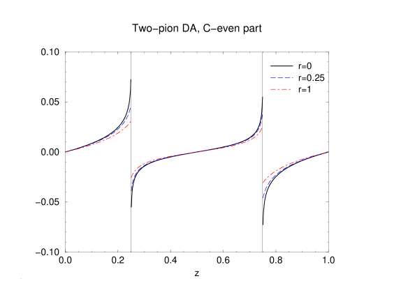
Figure 3: The $C$-even part of the two-pion distribution amplitude (33) at $\zeta=0.25$ and $s=20$ GeV² with various values of the cutoff parameter $r$ described in the text. The renormalization scale in $\alpha_{s}$ is chosen to be $s/4$.

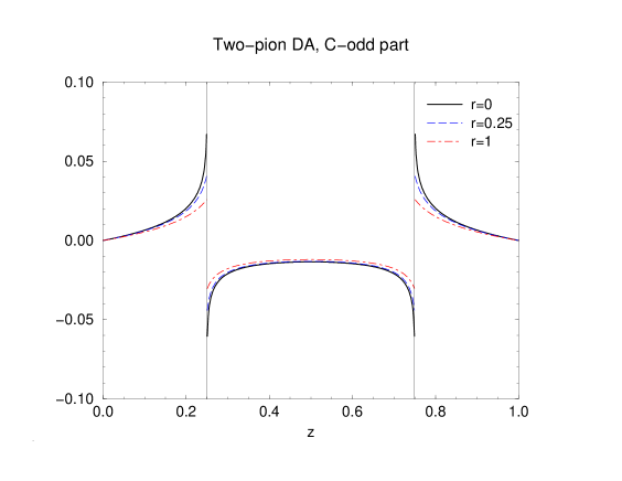
Figure 4: The $C$-odd part of the two-pion distribution amplitude (33). Parameters are as in Fig. 3.

The result (33) can easily be extended to more complicated single-pion distribution amplitudes. Using standard integrals it is possible to find the analytical form of the two-pion distribution amplitude including an arbitrary number of terms in the expansion (14). For the $a_{2}$-term for instance the integral (24) reads

$$I(z,\zeta,s)=36\,a_{2}\,\frac{\alpha_{s}}{s}\,\bigg{[}-\frac{1}{12}+5\bigg{(}\frac{z}{2\zeta}-\frac{z^{2}}{\zeta^{2}}\bigg{)}-\bigg{(}\frac{z}{\zeta}-5\frac{z^{2}}{\zeta^{2}}+5\frac{z^{3}}{\zeta^{3}}\bigg{)}\ln\frac{z-\zeta}{z}\bigg{]}.$$ (35)

We must now comment on the logarithmic singularities at $z=\zeta$ of the two-pion distribution amplitude (27), which are manifest in (33) and (35) and due to the fact that at that point the integral $I(z,\zeta,s)$ in (24) is divergent. They can be traced back to the singularity of $l\cdot q^{\prime}$ in the light-cone gauge gluon propagator (16) and show up as the denominator $\bar{x}u+yt$ in the hard-scattering amplitude $T_{H}^{u,B1}$ of eq. (18). This denominator cancels if one adds to (18) the contribution from diagrams B2, hence no divergence is encountered in the $\gamma^{*}\gamma$ amplitude given by (13). We have however made different variable substitutions in $T_{H}^{u,B1}$ and $T_{H}^{u,B2}$ in order to extract the two-pion distribution amplitude, and after this the cancellation no longer takes place.

Physically, the point $z=\zeta$ corresponds to the situation where one of the intrinsic quarks in a pion carries all of the pion’s momentum whereas the other quark has zero four-momentum, cf. eqs. (19) and (20). Of course, such a situation is unphysical and due to the limit of massless partons in combination with the collinear approximation employed when calculating the hard-scattering amplitude. The singularity in $\Phi_{2\pi}(z,\zeta,s)$ is a particular manifestation of the end-point singularities one encounters in the collinear hard-scattering approach, a problem that has been hotly debated for years [18]. In many applications, such as the $\gamma^{*}\gamma$ amplitude ${\cal M}_{\lambda\lambda^{\prime}}$, these singularities are canceled by the end-point zeroes of the distribution amplitudes $\phi_{\pi}$, and the result is finite. Note, however, that if $s$ is not large enough this result is strongly sensitive to the end-point regions, where the collinear approximation breaks down and perturbative QCD cannot be reliably used because the particle virtualities are small. In the case of the two-pion distribution amplitude the situation is even worse, since for $z=\zeta$ not all end-point singularities are canceled. For $z$ close to $\zeta$ the collinear hard-scattering approach can thus not be applied to the hadronic matrix element $\Phi_{2\pi}(z,\zeta,s)$ itself.

In order to understand this point on a more quantitative level, let us introduce for the moment a regularization for the integral (24) that cuts off the region where the longitudinal parton momenta are soft, i.e. where $x$ or $\bar{x}$ are smaller than $\Lambda^{2}/s$. Thus we replace the integration limits 0 and 1 in (24) by $r\,\Lambda^{2}/s$ and $1-r\,\Lambda^{2}/s$, respectively, where $r$ is a parameter that can be varied in order to investigate the sensitivity to the cutoff. In the limit $z\to\zeta$ the integral generates a logarithmic singularity $\propto\ln(\Lambda^{2}/s)$ which cancels the logarithm in the running coupling $\alpha_{s}$. One is thus left with an expression at leading-power level $1/s$ that formally is not of order $\alpha_{s}$. This should be taken as an indication that in the limit considered the two-pion distribution amplitude (27) is still sensitive to soft physics which cannot be accounted for in the standard hard-scattering picture. As already explained, in the $\gamma^{*}\gamma$ amplitude the logarithmic singularity drops out after integration over $z$ in (23), and our cutoff procedure only yields true power corrections of order $\Lambda^{2}/s$, which go beyond the accuracy of the hard-scattering approximation and can be neglected for sufficiently large $s$. Setting $\Lambda=1$ GeV, $r=1$, and taking the asymptotic single-pion distribution amplitude (32) we find for example at $s=20$ GeV² that ${\cal M}_{\lambda\lambda^{\prime}}$ decreases by 10% compared with the result for no cutoff. A similar suppression of the amplitude arises when the endpoint regions of the $z$-integration in (23) are cut off.

In Figs. 3 and 4 we show the results of our cutoff regularization for the two-pion distribution amplitude, with $\Lambda=1$ GeV and different values of $r$. We see that the results are sensitive to soft physics around $z=\zeta$, and become stable when $z$ is sufficiently far away from $\zeta$. From our discussion above it is natural to expect that the hard-scattering calculation becomes reliable when $|z-\zeta|$ is large compared with $\Lambda^{2}/s$.

Let us finally comment on the question of factorization scales. At which scale the single-pion distribution amplitudes in (23) and (24) should be taken is a priori not clear, since there are two large scales $s$ and $Q^{2}$ present in the hard-scattering diagrams. Likewise there is the question of the factorization scale in the two-pion distribution amplitude we have identified. The answer would require an analysis of the $\alpha_{s}$-corrections to the diagrams we have calculated here. Notice that at that level the two pions can not only originate from $q\bar{q}$ but also from a gluon pair, and that the ERBL evolution of the two-pion distribution amplitude for quarks mixes with the one for gluons [2]. One does therefore not expect a simple relation between the factorization scales of $\phi_{\pi}$ and of $\Phi_{2\pi}$ in (27). We also note that our results in Figs. 3 and 4, obtained with the asymptotic expression of $\phi_{\pi}(x)$, are far away from the asymptotic form of the two-pion distribution amplitude, whose $z$-dependence is given by $\Phi_{2\pi}^{+}\sim z(1-z)(2z-1)$ and $\Phi_{2\pi}^{-}\sim z(1-z)$.

4. To summarize: We have shown how to obtain the two-pion light-cone distribution amplitude in the perturbative limit, where both squared c.m. energy $s$ and photon virtuality $Q^{2}$ are large such that $\Lambda^{2}\ll s\ll Q^{2}$, where $\Lambda$ is of the order of 1 GeV. Working in the collinear hard-scattering picture we have identified the diagrams with handbag topology as the leading Feynman graphs and expressed the two-pion distribution amplitude in terms of the ordinary single-pion distribution amplitudes. Using light-cone gauge, we have explicitly checked that a gluon attached to the hard part of these diagrams leads to a suppression by a factor $1/Q$. This is in accordance with general theory, where it is well known that contributions from transverse gluons are power suppressed, whereas scalar and longitudinal gluons can be eliminated by choosing an appropriate gauge. In this approach we have been able to reproduce the scaling behavior and helicity selection rule of the process. We have verified the charge conjugation relation and the polynomiality condition for the two-pion distribution amplitude, and that its first moment equals the timelike pion form factor. Like the latter, our two-pion distribution amplitude falls like $1/s$, and to leading order in $\alpha_{s}$ is purely real.

Using expression (33) for the two-pion distribution amplitude we can write the amplitude for the process under consideration in the following simple form:

$${\cal M}_{\lambda\lambda^{\prime}}(\zeta,s)=\delta_{\lambda\lambda^{\prime}}\,e^{2}(e_{u}^{2}+e_{d}^{2})\,\frac{8\pi f_{\pi}^{2}\,\alpha_{s}}{s}\,\bigg{[}\frac{1}{\zeta}\ln\frac{1}{\bar{\zeta}}+\frac{1}{\bar{\zeta}}\ln\frac{1}{\zeta}\bigg{]},$$ (36)

where $\zeta$ must be sufficiently far from 0 and 1 to ensure $-t,-u\gg\Lambda^{2}$.

We are aware that, at this stage, the investigations presented in this work are above all theoretically motivated, since it will be difficult to obtain experimental data for the process $\gamma^{*}\gamma\to\pi^{+}\pi^{-}$ in the kinematical region we have considered. However, we have seen how two different types of factorization merge in the region where they are both applicable, and know the form which any model two-pion distribution amplitude, for instance the one proposed in [7], has to approach at large $s$.

Acknowledgments: This work is partially supported by the U.S. Department of Energy, contract DE-AC03-76SF00515, and M.D. acknowledges support by the Alexander von Humboldt Foundation. C.V. thanks the Deutsche Forschungsgemeinschaft for a graduate grant and furthermore M. Polyakov and C. Weiss for useful discussions.

References

- [1] D. Müller, D. Robaschik, B. Geyer, F.M. Dittes and J. , Fortschr. Phys. 42, 101 (1994), hep-ph/9812448.
- [2] M. Diehl, T. Gousset, B. Pire and O. Teryaev, Phys.Rev.Lett. 81, 1782 (1998), hep-ph/9805380.
- [3] X. Ji, Phys. Rev. Lett. 78, 610 (1997), hep-ph/9603249; Phys. Rev. D55, 7114 (1997), hep-ph/9609381.
- [4] A.V. Radyushkin, Phys. Lett. B380, 417 (1996), hep-ph/9604317; Phys. Rev. D56, 5524 (1997), hep-ph/9704207.
- [5] A.Freund, hep-ph/9903489.
- [6] M.V. Polyakov, Nucl. Phys. B555, 231 (1999), hep-ph/9809483.
- [7] M.V. Polyakov and C. Weiss, Phys. Rev. D59, 091502 (1999), hep-ph/9806390.
- [8] G.P. Lepage and S.J. Brodsky, Phys. Rev. D22, 2157 (1980).
- [9] S.J. Brodsky and G.P. Lepage, Phys. Rev. D24, 1808 (1981).
- [10] J.F. Gunion, D. Miller and K. Sparks, Phys. Rev. D33, 689 (1986).
- [11] A.V. Efremov and A.V. Radyushkin, Theor. Mat. Phys. 42, 97 (1980).
-
[12]
X. Ji, J. Phys. G24, 1181 (1998),
hep-ph/9807358;
A.V. Radyushkin, Phys. Lett. B449, 81 (1999), hep-ph/9810466. - [13] CLEO Collaboration, Phys. Rev. D57, 33 (1998), hep-ex/9707031.
-
[14]
I.V. Musatov and A.V. Radyushkin, Phys. Rev. D56, 2713 (1997), hep-ph/9702443;
P. Kroll and M. Raulfs, Phys. Lett. B387, 848, (1996), hep-ph/9605264. - [15] R. Jakob, P. Kroll and M. Raulfs, J. Phys. G22, 45 (1996), hep-ph/9410304.
- [16] T. Feldmann, hep-ph/9907491 (to be published in Int. J. Mod. Phys. A).
- [17] J.C. Collins, L. Frankfurt and M. Strikman, Phys.Rev. D56, 2982 (1997), hep-ph/9611433.
-
[18]
N. Isgur and C.H. Llewellyn Smith, Phys. Rev. Lett. 52, 1080 (1984); Phys. Lett. B217, 535 (1989);
A.V. Radyushkin, Nucl.Phys. A527, 153c (1991).