Quark-antiquark potential in the analytic approach to QCD

Abstract

The quark-antiquark potential is constructed by making use of a new analytic running coupling in QCD. This running coupling arises under “analytization” of the renormalization group equation. The rising behavior of the quark-antiquark potential at large distances, which provides the quark confinement, is shown explicitly. At small distances, the standard behavior of this potential originating in the QCD asymptotic freedom is revealed. The higher loop corrections and the scheme dependence of the approach are briefly discussed.

I Introduction

The description of quark dynamics inside hadrons remains an actual problem of elementary particle theory. The asymptotic freedom in quantum chromodynamics (QCD) enables one to investigate the quark interactions at small distances by making use of standard perturbation theory. The quark dynamics at large distances (the confinement region) lies beyond such calculations. For this purpose other approaches are used: phenomenological potential models [1], string models [2], bags models [3], lattice calculations [4], the explicit account of nontrivial QCD vacuum structure [5], and variational perturbation theory [6].

Recently Shirkov and Solovtsov proposed a new analytic approach to QCD [7]. Its basic idea is the explicit imposition of the causality condition, which implies the requirement of the analyticity in the $Q^{2}$ variable for the relevant physical quantities. The essential merits of this approach are the following: absence of unphysical singularities at any loop level, stability in the infrared (IR) region, stability with respect to loop corrections, and extremely weak scheme dependence. The analytic approach has been applied successfully to such problems as the $\tau$ lepton decays, $e^{+}e^{-}$-annihilation into hadrons, sum rules (see [8] and references therein).

In Refs. [9, 10] the analytic approach has been employed to the solution of the renormalization group (RG) equation. The analyticity requirement was imposed on the RG equation itself, before deriving its solution. Solving the RG equation, “analytized” (i.e., requiring analyticity) in the above-mentioned way, one gets, at one-loop level, a new analytic running coupling, which possesses practically the same appealing features as the Shirkov-Solovtsov running coupling [7] does. An essential distinction, that will play a crucial role in the present paper, is the IR singularity of the new analytic running coupling at the point $q^{2}=0$. It should be stressed here that such a behavior of the invariant charge is in a complete agreement with the Schwinger-Dyson equations, and, as it will be demonstrated in Sec. III, provides the quark confinement (see Sec. II for the details).

In this paper we shall adhere to the model [5, 11] of obtaining the quark-antiquark ($q\bar{q}$) potential by the Fourier transformation of the running coupling. However, the perturbative running coupling ${\alpha}_{\text{s}}(q^{2})$ does not enable one to obtain the rising $q\bar{q}$ potential without invoking additional assumptions [11].

The objective of this paper is to construct the quark-antiquark potential by making use of the new analytic running coupling. This potential proves to be rising at large distances (i.e., providing the quark confinement) and, at the same time, it incorporates the asymptotic freedom at small distances. It is essential that for obtaining this potential no additional assumptions, lying beyond the standard RG method in the quantum field theory and the analyticity requirement, will be used.

The layout of the paper is as follows. In Sec. II the derivation of the new analytic running coupling is presented and its properties are briefly discussed. In Sec. III the quark-antiquark potential, generated by the new analytic running coupling, is derived by making use of the Fourier transformation. Further, the asymptotic behavior of the potential at large and small distances is investigated. In Sec. IV the higher loop corrections and the scheme dependence of the potential are discussed briefly. For practical purposes, a simple approximate formula for the potential is proposed which interpolates its infrared and ultraviolet asymptotics. This formula is compared with the phenomenological Cornell potential. Proceeding from this, an estimation of the QCD parameter $\Lambda$ is obtained. In the Conclusion (Sec. V) the obtained results are formulated in a compact way, and the further studies in this approach are outlined.

II A new model for the QCD analytic running coupling

In the analytic approach to QCD, proposed by Shirkov and Solovtsov [7], the basic idea is the explicit imposing of the causality condition, which implies the requirement of the analyticity in the $Q^{2}$ variable for the relevant physical quantities. Later this idea was applied to the “analytization” (i.e., the procedure of analyticity requirement) of the perturbative series when calculating the QCD observables [8]. The results turned out to be quite encouraging. As was mentioned in the Introduction, the analytization of the perturbative series leads to the elimination of the unphysical singularities, to the higher loop correction stability and to a weak scheme dependence. However, the $Q^{2}$-evolution of some QCD observables (for instance, the structure function moments) is intimately tied with the solution of the RG equation. Our task here is to involve the analytization procedure into the RG formalism more profoundly.

Let us consider the RG equation of a quite general form for a quantity ${\sf A}(Q^{2})$ (it may be, for example, the gluon propagator, or the structure function moment). At the one-loop level this equation reads

$$\frac{d\ln{\sf A}(Q^{2})}{d\ln Q^{2}}=\gamma\,\widetilde{\alpha}^{(1)}_{\text{s}}(Q^{2}),$$ (1)

where $\gamma$ is the corresponding anomalous dimension (the negative noninteger number in the general case), $\widetilde{\alpha}^{(1)}_{\text{s}}(Q^{2})=1/\ln(Q^{2}/\Lambda^{2})$ is the one-loop perturbative running coupling. The solution of Eq. (1) can be written in the form

$${\sf A}(Q^{2})={\sf A}(Q^{2}_{0})\left[\frac{\widetilde{\alpha}^{(1)}_{\text{s}}(Q^{2}_{0})}{\widetilde{\alpha}^{(1)}_{\text{s}}(Q^{2})}\right]^{\gamma}.$$ (2)

From here it follows immediately, that this solution has unphysical singularities in the physical region $Q^{2}>0$. However, in many interesting cases mentioned above, the quantity ${\sf A}(Q^{2})$ must have correct analytic properties in the $Q^{2}$ variable (namely, there is the only cutoff $Q^{2}\leq 0$). One can demonstrate this proceeding from the first principles. So, for the gluon propagator this assertion follows from the causal Källén-Lehmann representation (see, e.g., [12]), and for the structure function moments this is a consequence of the Deser-Gilbert-Sudarshan integral representation (see, e.g., [13]). Thus, we come to a contradiction.

The point, which is crucial to our consideration, is the following. The RG equation in the form (1) involves, in fact, a contradiction. The left-hand side of this equation has no unphysical singularities in the $Q^{2}>0$ region, while its right-hand side has pole-type singularity at the point $Q^{2}=\Lambda^{2}$. The account of the higher loop contributions just introduces the additional unphysical singularities of the cut type in the physical region $Q^{2}>0$ and hence does not solve the problem.

In order to avoid this contradiction, we propose to use the following method [9, 10]. Before solving the RG equation (1) one should analytize its right-hand side as a whole. This prescription leads to the analytized RG equation, which, at the one-loop level, takes the form

$$\frac{d\ln{\sf A}(Q^{2})}{d\ln Q^{2}}=\gamma\,\widetilde{\alpha}^{(1)}_{\text{an}}(Q^{2}),$$ (3)

where $\widetilde{\alpha}^{(1)}_{\text{an}}(Q^{2})=1/\ln(Q^{2}/\Lambda^{2})+1/(1-Q^{2}/\Lambda^{2})$ is the perturbative running coupling analytized by making use of the Shirkov-Solovtsov prescription [7]. The solution of Eq. (3) can be presented in the form

$${\sf A}(Q^{2})={\sf A}(Q^{2}_{0})\left[\frac{{}^{\text{N}}\widetilde{\alpha}^{(1)}_{\text{an}}(Q^{2}_{0})}{{}^{\text{N}}\widetilde{\alpha}^{(1)}_{\text{an}}(Q^{2})}\right]^{\gamma},$$ (4)

where

$$^{\text{N}}\widetilde{\alpha}^{(1)}_{\text{an}}(Q^{2})=\frac{z-1}{z\ln z},\quad z=\frac{Q^{2}}{\Lambda^{2}}.$$ (5)

Comparing the solution (4) with Eq. (2) one infers that ${}^{\text{N}}\alpha^{(1)}_{\text{an}}(Q^{2})$ should be treated as a new one-loop analytic running coupling. Really, it possesses the same properties, as the one-loop running coupling analytized through the Shirkov-Solovtsov procedure. Namely, the new running coupling has the standard asymptotic behavior at $z\to\infty$ and it has no unphysical singularities in the $Q^{2}>0$ region. The latter follows directly from the causal representation of the Källén-Lehmann type, that holds for ${}^{\text{N}}\widetilde{\alpha}^{(1)}_{\text{an}}(Q^{2})$:

$$^{\text{N}}\widetilde{\alpha}^{(1)}_{\text{an}}(Q^{2})=\int_{0}^{\infty}\frac{{}^{\text{N}}\rho(\sigma)}{\sigma+z}d\sigma,\quad^{\text{N}}\rho(\sigma)=\left(1+\frac{1}{\sigma}\right)\frac{1}{\ln^{2}\sigma+\pi^{2}}.$$ (6)

The distinctive feature of the new running coupling, which will play the crucial role in the framework of our consideration, is its singularity at the point $Q^{2}=0$. It is worth noting that such a behavior of the invariant charge is in a complete agreement with the Schwinger-Dyson equations (see discussion in Ref. [14]), and, as it will be demonstrated in the next section, provides the quark confinement.

Summarizing all stated above, we propose the following model for the analytic running coupling. We define the new analytic running coupling ${}^{\text{N}}\alpha_{\text{an}}(Q^{2})$ as the solution of the analytized RG equation at the respective loop level. Here one has to choose the anomalous dimensions in such a way that the solution of the standard RG equation is the perturbative running coupling at the loop level considered. Thus, at the one-loop level, the new analytic running coupling has the form [9, 10]

$$^{\text{N}}\alpha^{(1)}_{\text{an}}(Q^{2})=\frac{4\pi}{\beta_{0}}\frac{z-1}{z\ln z},\quad z=\frac{Q^{2}}{\Lambda^{2}},$$ (7)

where $\beta_{0}=11-2\,n_{f}/3$ is the first coefficient of the $\beta$-function. At the higher loop levels there is only the integral representation for ${}^{\text{N}}\alpha_{\text{an}}(Q^{2})$. So, at the $i$-loop level we have

$$^{\text{N}}\alpha^{(i)}_{\text{an}}(Q^{2})=~{}^{\text{N}}\alpha^{(i)}_{\text{an}}(Q^{2}_{0})\frac{z_{0}}{z}\exp\left[\int_{0}^{\infty}\frac{\rho^{(i)}(\sigma)}{\sigma}\ln\left(\frac{\sigma+z}{\sigma+z_{0}}\right)d\sigma\right],$$ (8)

where $\rho^{(i)}(\sigma)=\left[\widetilde{\alpha}^{(i)}_{\text{s}}(-\sigma-i\varepsilon)-\widetilde{\alpha}^{(i)}_{\text{s}}(-\sigma+i\varepsilon)\right]/(2\pi i)$ is the spectral density, and $z_{0}=Q^{2}_{0}/\Lambda^{2}$ is the normalization point.

Figure 1 shows the new analytic running coupling computed at the one-, two-, and three-loop levels. It is clear from this figure that our analytic running coupling possesses the higher loop stability. Moreover, it can be shown that the singularity of the new analytic running coupling at the point $Q^{2}=0$ is of the universal type at any loop level. This is clear from the following simple consideration. When $z\to 0$ the basic contribution into Eq. (8) affords the integration over the small $\sigma$ region. The spectral density $\rho^{(i)}(\sigma)$ at any loop level has the same limit when $\sigma\to 0$: $\rho^{(i)}(\sigma)\to\rho^{(1)}(\sigma)=(\ln^{2}\sigma+\pi^{2})^{-1}$ [8]. Hence the new analytic running coupling (8) has the unique behavior when $z\to 0$.

III Quark-antiquark potential generated by the new analytic running coupling

Here we are going to use the new analytic running coupling for obtaining the interquark potential. We proceed from the standard expression [5, 11] for the $q\bar{q}$ potential in terms of the running coupling $\alpha(q^{2})$,

$$V(r)=-\frac{16\pi}{3}\int_{0}^{\infty}\frac{\alpha(q^{2})}{q^{2}}\frac{e^{i{\bf qr}}}{(2\pi)^{3}}\,d{\bf q}.$$ (9)

For the construction of the new interquark potential ${}^{N}V(r)$ we shall use the new analytic running coupling (7)

$$^{\text{N}}\alpha_{\text{an}}(Q^{2})=\frac{4\pi}{\beta_{0}}\frac{z-1}{z\ln z},\quad z=\frac{Q^{2}}{\Lambda^{2}}.$$ (10)

Upon the integration over the angular variables and the substitution $q/\Lambda\to q,\,r\Lambda\to R$ in Eq. (9), one gets

$$^{N}V(r)=-\frac{32}{3\beta_{0}}\Lambda\cdot\widetilde{V}(R),\quad R=\Lambda r,$$ (11)

where

$$\widetilde{V}(R)=\int_{0}^{\infty}\frac{q^{2}-1}{q^{2}\ln q^{2}}\frac{\sin(qR)}{qR}\,dq$$ (12)

is the dimensionless potential.

In order to perform the integration in Eq. (12) we consider the auxiliary function

$$I(n,R)=\lim_{a\to 0+}\int_{0}^{\infty}\frac{q^{n-1}}{\ln(a+q^{2})}\sin(qR)\,dq.$$ (13)

Here the parameter $a$ is introduced for shifting the origin of the cut along the imaginary axis Im $q$. It is obvious that

$$\widetilde{V}(R)=\frac{1}{R}\left[I(0,R)-I(-2,R)\right].$$ (14)

For even $n$ the integrand in Eq. (13) is an even function of $q$. Therefore

$$I(n,R)=\frac{1}{2}\>\mbox{\rm Im}\,\lim_{a\to 0+}J(n,a,R),$$ (15)

where

$$J(n,a,R)={\cal P}\!\!\int_{-\infty}^{\infty}\!\!F(q)\,dq,\quad F(q)=\frac{q^{n-1}e^{iqR}}{\ln(a+q^{2})}.$$ (16)

The sign ${\cal P}$ means the principal value of the integral.

The function $F(q)$ in Eq. (16) has the cuts $(-i\infty,-i\sqrt{a}]$, $\,[i\sqrt{a},i\infty)$ and simple poles at the points $q=\mp\sqrt{1-a}$. Let us consider the integral of the function $F$ along the contour $\Gamma$ shown in Fig. 2. The function $F(q)$ has no singularities inside the contour $\Gamma$, therefore $\oint_{\Gamma}\!F\,dq=0$. Contribution to this integral of the semicircle of infinitely large radius in upper half-plane (see Fig. 2) vanishes. Performing the integration along the two semicircles $c_{-}$ and $c_{+}$ of the vanishing radius and along the cut $C$ on the imaginary axis, we obtain

$$J(n,a,R) = i\pi\Biggl{\{}\frac{1}{2}\left[(\sqrt{1-a})^{n-2}e^{iR\sqrt{1-a}}\right.$$ (19)

$$+\left.(-\sqrt{1-a})^{n-2}e^{-iR\sqrt{1-a}}\right]$$

$$+2i^{n-2}\int_{\sqrt{a}}^{\infty}\frac{x^{n-1}e^{-Rx}}{\ln^{2}(x^{2}-a)+\pi^{2}}\,dx\Biggr{\}}.$$

Hence, for even $n$ the function $I(n,R)$ in Eq. (13) takes the form

$$I(n,R)=\pi\left[\frac{1}{2}\cos R-(-1)^{n/2}{\cal N}(R,n)\right],$$ (20)

where

$${\cal N}(R,n)=\int_{0}^{\infty}\frac{x^{n-1}e^{-Rx}}{\ln^{2}(x^{2})+\pi^{2}}\,dx.$$ (21)

It is rather complicated to perform the integration in Eq. (21) explicitly. Therefore we address the study of the asymptotics. First of all, we would like to know whether the $q\bar{q}$ potential ${}^{N}V(r)$ in Eq. (11) provides the quark confinement. For the investigation of the potential behavior at large distances it is enough to consider the asymptotic of the function ${\cal N}(R,n)$ in Eq. (21) when $R\to\infty$. This function can be represented in the following way

$${\cal N}(R,n)=(-1)^{n}\frac{\partial^{n}}{\partial R^{n}}\int_{0}^{\infty}\frac{e^{-Rx}}{x\left[\ln^{2}(x^{2})+\pi^{2}\right]}\,dx.$$ (22)

At large $R$ the basic contribution into Eq. (22) gives the integration over the small $x$ region. Let us transform ${\cal N}(R,n)$ identically:

$${\cal N}(R,n)=\frac{\partial^{n}}{\partial R^{n}}\int_{0}^{\infty}\frac{(-1)^{n}e^{-Rx}}{4x(\ln^{2}x+\pi^{2})}\left[1+\frac{3L}{1+L}\right]dx,$$ (23)

where $L=\pi^{2}/(4\ln^{2}x)$. Neglecting the second term in the square brackets in Eq. (23), we use the formula (4.361.2) from Ref. [15]:

$$\int_{0}^{\infty}\frac{e^{-\mu x}}{x(\ln^{2}x+\pi^{2})}dx=e^{\mu}-\nu(\mu),\quad\mbox{\rm Re}\;\mu>0,$$ (24)

where $\nu(\mu)$ is the so-called transcendental $\nu$-function [16]:

$$\nu(\mu)=\int_{0}^{\infty}\frac{\mu^{t}dt}{\Gamma(t+1)}.$$ (25)

Eventually, we obtain for $R\to\infty$,

$${\cal N}(R,n)\simeq\frac{(-1)^{n}}{4}\left[e^{R}-\nu(R)+\int_{0}^{-n}\frac{R^{t}dt}{\Gamma(t+1)}\right].$$ (26)

Taking into account Eqs. (14), (20), and (26) one can present the quark-antiquark potential (11) at large $R$ in the following way:

$$^{N}V(r)\simeq\frac{8\pi}{3\beta_{0}}\frac{\Lambda}{R}\left[2\left(e^{R}-\nu(R)\right)+\int_{0}^{2}\frac{R^{t}dt}{\Gamma(t+1)}\right].$$ (27)

The behavior of the potential ${}^{N}V(r)$ at $r\to\infty$ is determined by the last term in Eq. (27). Integration of this term by parts gives

$$\int_{0}^{2}\frac{R^{t}dt}{\Gamma(t+1)} = \frac{R^{2}}{2\ln R}\left[1+2\sum\limits_{k=1}^{\infty}\frac{f_{k}(2)}{\ln^{k}R}\right]$$ (29)

$$-\frac{1}{\ln R}\left[1+\sum\limits_{j=1}^{\infty}\frac{f_{j}(0)}{\ln^{j}R}\right],$$

where

$$f_{n}(t)=\left.\frac{d^{n}}{ds^{n}}\frac{(-1)^{n}}{\Gamma(s+1)}\right|_{s=t}.$$ (30)

In the limit $R\to\infty$, Eq. (29) takes the form

$$\int_{0}^{2}\frac{R^{t}dt}{\Gamma(t+1)}=\frac{R^{2}}{2\ln R}.$$ (31)

Therefore the quark-antiquark potential ${}^{N}V(r)$ proves to be rising at large distances

$$^{N}V(r)\simeq\frac{8\pi}{3\beta_{0}}\Lambda\cdot\frac{1}{2}\frac{\Lambda r}{\ln(\Lambda r)},\quad r\to\infty.$$ (32)

Thus the new analytic running coupling ${}^{\text{N}}{\alpha}_{\text{an}}(q^{2})$ [see Eq. (7)] leads to the rising quark-antiquark potential ${}^{N}V(r)$ which can, in principle, describe the quark confinement.

It is important to point out that the behavior of the potential ${}^{N}V(r)$ when $r\to 0$ has the standard form determined by the asymptotic freedom (see, e.g., Ref. [11]),

$$^{N}V(r)\simeq\frac{8\pi}{3\beta_{0}}\Lambda\cdot\frac{1}{\Lambda r\ln(\Lambda r)},\quad r\to 0.$$ (33)

Unfortunately, it is impossible to obtain the explicit dependence ${}^{N}V(r)$ for the whole region $0<r<\infty$. A simple interpolating formula, which can be applied for practical use, will be given in the next section.

IV Discussion

Let us discuss briefly the higher loop contribution. As was mentioned in the Sec. II, the singularity of $i$-loop analytic running coupling ${}^{\text{N}}\alpha^{(i)}_{\text{an}}(q^{2})$ at the point $q=0$ is of the universal type at any loop level. Therefore, when $q\to 0\,$ we have ${}^{\text{N}}\alpha^{(i)}_{\text{an}}(q^{2})\sim\,^{\text{N}}\alpha^{\text{(1)}}_{\text{an}}(q^{2})\,C^{i}$, where $C^{i}$ are constants. Taking into account that the maximal difference between ${}^{\text{N}}\alpha^{(i)}_{\text{an}}(q^{2})$ and ${}^{\text{N}}\alpha^{\text{(1)}}_{\text{an}}(q^{2})$ is in the small $q^{2}$ region, we arrive at the following conclusion. The account of the higher loop corrections leads to changing the slope of the $q\bar{q}$ potential ${}^{N}V(r)$ when $r\to\infty$. This corresponds to a simple redefinition of the parameter $\Lambda$ in Eq. (32) at the higher loop levels.

As far as the scheme dependence of this approach, we have to point out the following. It was shown in [9] that the solutions of the analytized RG equation at the higher loop level have extremely weak scheme dependence. In particular, the solutions of the RG equation with $\overline{\text{MS}}$ and MS schemes, are practically coinciding. Hence, at the higher loop level (there is no scheme dependence at the one-loop level), the use of different subtraction schemes leads to the slight variation of the $q\bar{q}$ potential.

Thus, neither higher loop corrections, nor scheme dependence, can affect qualitatively the result obtained in the previous section.

For the practical use of the new potential it is worth obtaining a simple explicit expression that approximates it sufficiently well. For this purpose one can use, for instance, the approximating function

$$U(r) = \frac{8\pi}{3\beta_{0}}\Lambda\left[\frac{1}{\ln R}\left(\frac{1}{R}+\frac{R}{2}\right)+\frac{1}{1-R}\left(\frac{3}{2}+Rf_{1}(2)\right)\right.$$ (35)

$$\left.+Rf_{1}(2)\left(\frac{1}{\ln^{2}R}-\frac{1}{(R-1)^{2}}+\frac{11}{12}\right)\right],$$

which has no any unphysical singularities and possesses the asymptotics (32) and (33). This function is obtained by smooth sewing the asymptotics

$${}^{N}V(r) \simeq \frac{8\pi}{3\beta_{0}}\Lambda\cdot\left[\frac{R}{2\ln(R)}+\frac{Rf_{1}(2)}{\ln^{2}(R)}\right],\quad R\to\infty,\nopagebreak$$ (36)

$${}^{N}V(r) \simeq \frac{8\pi}{3\beta_{0}}\Lambda\cdot\frac{1}{R\ln(R)},\quad R\to 0,\quad R=\Lambda r.$$ (37)

The formula (36) keeps explicitly the second leading term of the expansion (29), $f_{1}(2)=0.461$. Some terms have been introduced into Eq. (35) only for eliminating the singularity at the point $R=1$. It should be mentioned here that the next terms in the expansion (29) practically do not affect the shape of $U(r)$. Of course, the function (35) is not the unique interpolating function between asymptotics (36) and (37). Nevertheless, the comparison of $U(r)$ with the phenomenological potential

$$^{C}V(r)=-\frac{4}{3}\frac{a}{r}+\sigma r+\mbox{const}$$ (38)

(the so-called Cornell potential [1]) shows their almost complete coincidence (see Fig. 3). The fit has been performed with the use of the least square method in the physical meaning region $0.1\leq r\leq 1.0$ fm [5]. The varied parameter in Eq. (35) is $\Lambda$. The possibility of shifting the potential ${}^{C}V(r)$ in Eq. (38) by a constant was also used. A rough estimation of $\Lambda$ in the course of this fitting gives $\Lambda\simeq 500$ MeV. This is in agreement with the values obtained earlier in the framework of the analytic approach to QCD [8].

V Conclusion

In the paper the quark-antiquark potential is constructed by making use of the new analytic running coupling in QCD. This running coupling arises under analytization of the renormalization group equation before its solving. The rising behavior of the quark-antiquark potential at large distances, which provides the quark confinement, is shown explicitly. The key property of the new analytic running coupling, leading to the confining potential, is its infrared singularity at the point $q^{2}=0$. At small distances, the standard behavior of the potential, originating in the QCD asymptotic freedom, is revealed. It is also demonstrated that neither higher loop corrections, nor scheme dependence, can affect qualitatively the obtained result. The estimation of the parameter $\Lambda$ in this approach gives a reasonable value, $\Lambda\simeq 500$ MeV.

In further studies it would undoubtedly be interesting to consider in this approach the dependence of the $q\bar{q}$ potential on the quark masses.

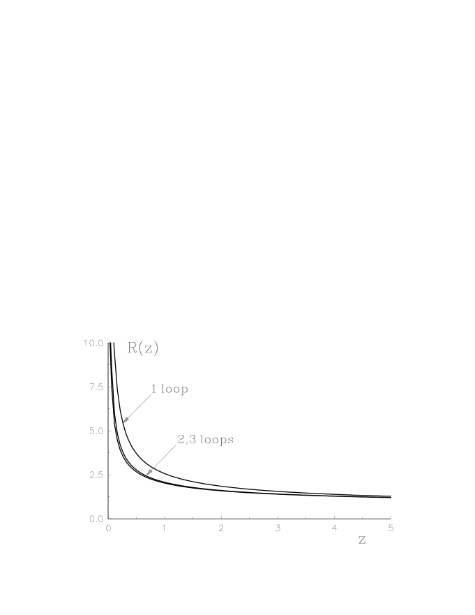
FIG. 1.: The normalized new analytic running coupling $R(z)=~{}^{\text{N}}\widetilde{\alpha}_{\text{an}}(Q^{2})/~\!{}^{\text{N}}\widetilde{\alpha}_{\text{an}}(Q^{2}_{0})$ at the one-, two-, and three-loop levels. The normalization point is $Q^{2}_{0}=10\Lambda^{2}$, $\,z=Q^{2}/\Lambda^{2}$.

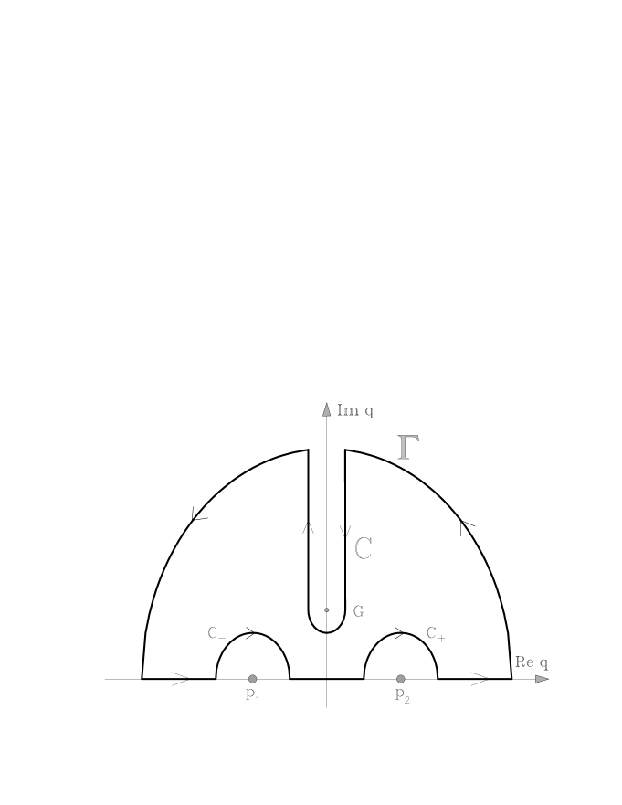
FIG. 2.: The integration contour in the complex $q$-plane. The notations are: $p_{1}=-\sqrt{1-a},\;$ $p_{2}=\sqrt{1-a},\;$ G= $i\sqrt{a}$.

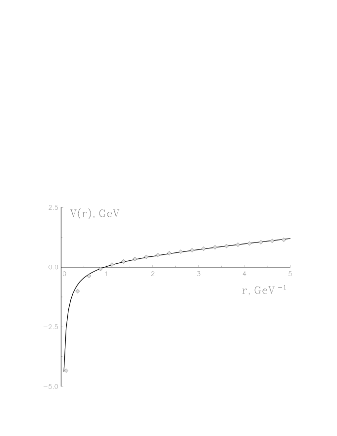
FIG. 3.: Comparison of the potential $U(r)$ given by Eq. (35) (solid curve) with the phenomenological Cornell potential ($\diamond$), Eq. (38). The values of the parameters are: $a=0.39$, $\sigma=0.182$ GeV² [5], $\Lambda=530\,$MeV, $n_{f}=5$.

- [1] E. Eichten et al., Phys. Rev. D 17, 3090 (1978); A. Martin, Phys. Lett. 93B, 338 (1980); C. Quigg and J. L. Rosner, ibid. 71B, 153 (1977).
- [2] B. M. Barbashov and V. V. Nesterenko, Introduction to the Relativistic String Theory (World Scientific, Singapore, 1990).
- [3] P. Hasenfratz and J. Kuti, Phys. Rep., Phys. Lett. 40C, 75 (1978); S. Adler and T. Piran, Rev. Mod. Phys. 56, 1 (1984).
- [4] G. S. Bali, C. Schlichter, and K. Schilling, Phys. Rev. D 51, 5165 (1995).
- [5] N. Brambilla and A. Vairo, “Quark Confinement and the Hadron Spectrum”, hep-ph/9904330.
- [6] I. L. Solovtsov, Phys. Lett. B 327, 335 (1994).
- [7] D. V. Shirkov and I. L. Solovtsov, Phys. Rev. Lett. 79, 1209 (1997); hep-ph/9704333.
- [8] I. L. Solovtsov and D. V. Shirkov, Theor. Math. Phys. 120, 482 (1999); hep-ph/9909305.
- [9] A. V. Nesterenko, Diploma thesis, Moscow State University, 1998.
- [10] A. V. Nesterenko, in Particle Physics on the Boundary of Millenniums, Proceedings of the 9th International Lomonosov Conference on Elementary Particle Physics, Moscow, Russia, 1999, edited by A. Studenikin (MSU and ICAS) (to be published).
- [11] J. L. Richardson, Phys. Lett. 82B, 272 (1979); R. Levine and Y. Tomozawa, Phys. Rev. D 19, 1572 (1979).
- [12] N. N. Bogolyubov and D. V. Shirkov, Introduction to the Theory of Quantized Fields (Interscience, New York, 1980).
- [13] W. Wetzel, Nucl. Phys. B139, 170 (1978).
- [14] A. I. Alekseev and B. A. Arbuzov, Mod. Phys. Lett. A 13, 1747 (1998); hep-ph/9704228.
- [15] I. S. Gradshteijn and I. M. Ryzhik, Table of Integrals, Series and Products (Academic, New York, 1994).
- [16] H. Bateman and A. Erdelyi, Higher Transcendental Functions (McGraw-Hill, New York, 1953-1955), Vol. 3.