Factorization scheme dependence
of the NLO inclusive jet cross section

Abstract

We study the factorization scheme dependence of the next-to-leading order inclusive one jet cross section $d\sigma/dE_{T}$. The scheme is varied parametrically along the direction that transforms the $\overline{\mathrm{MS}}$ scheme to the DIS scheme: we introduce a parameter $\lambda$ such that $\lambda=0$ is $\overline{\mathrm{MS}}$ and $\lambda=1$ is DIS. The factorization scale $\mu$ is also varied. We observe a change of $\pm 9\%$ in the cross section for $E_{T}=50\ \mathrm{GeV}$ when $\mu$ and $\lambda$ are varied in the range $-2\leq\lambda\leq 2$, $E_{T}/8\leq\mu\leq 2E_{T}$. This grows to $\pm 32\%$ for $E_{T}=400\ \mathrm{GeV}$.

Calculations in perturbative QCD involve conventions. For example, one conventionally uses the  MS  scheme for renormalization. Within the  MS  scheme, one needs to specify a renormalization scale $\mu_{\rm UV}$. If one does a calculation at next-to-next-to-leading order (NNLO), it is possible to vary the renormalization scheme by setting the third coefficient in the $\beta$ function, $b_{3}$. It is useful to study the dependence of the calculated cross sections on the chosen conventions. Thus, with a NNLO calculation of the total cross section for $e^{+}+e^{-}\to hadrons$, one can examine the dependence of the cross section on $\mu_{\rm UV}$ and $b_{3}$ [1]. Studies like this have a dual purpose. First, we learn about the extent to which our arbitrary choices affect the results. Second, we obtain an estimate, or at least an approximate lower bound, on the theoretical uncertainty in the calculated order $\alpha_{s}^{N}$ cross section arising from uncalculated terms of order $\alpha_{s}^{N+1}$ and higher. This is because among the uncalculated terms are contributions containing factors of $\ln(\mu_{\rm UV})$ and $b_{3}$ that cancel the $\mu_{\rm UV}$ and $b_{3}$ dependence in the calculated terms. We cannot find all of the $\alpha_{s}^{N+1}$ terms (since we lack the calculation), but at least we know the size of some of them.

In cross sections involving initial state hadrons, the theoretical formula contains parton distribution functions as factors. The calculated result at order $\alpha_{s}^{N}$ depends on the convention we use for collinear factorization. Put another way, the result depends on the definition of the parton distribution functions. In particular, the result depends on the factorization scale $\mu_{\rm coll}$ (the scale that appears in the parton distributions $f_{a/A}(x,\mu_{\rm coll})$). In NLO calculations of hard cross sections with initial state hadrons, it is common to examine the dependence of the result on $\mu_{\rm coll}$.

In this paper, we examine a bigger space of convention dependence. The dependence of the parton distribution functions on the factorization scale has the form

$$f_{a/A}(x,\tilde{\mu}) = f_{a/A}(x,\mu)$$ (3)

$$\mbox{}+{\alpha_{s}(\mu)\over 2\pi}\,\ln(\tilde{\mu}^{2}/\mu^{2})\int_{x}^{1}{d\xi\over\xi}\sum_{b}K^{(0)}_{ab}(x/\xi)\,f_{b/A}\!\left(\xi,\mu\right)$$

$$\mbox{}+{\cal O}(\alpha_{s}^{2}).$$

Here $K^{(0)}_{ab}(\xi)$ is the lowest order Altarelli-Parisi kernel. If we like, we can redefine the parton distributions according to

$$\tilde{f}_{a/A}(x,\mu) = f_{a/A}(x,\mu)$$ (5)

$$\mbox{}+{\alpha_{s}(\mu)\over 2\pi}\,\sum_{J=0}^{N}\lambda_{J}\int_{x}^{1}{d\xi\over\xi}\sum_{b}K^{(J)}_{ab}(x/\xi)\,f_{b/A}\!\left(\xi,\mu\right).$$

Here $K^{(0)}_{ab}(\xi)$ is still the Altarelli-Parisi kernel, so that if we put $\lambda_{0}=\ln\left(\tilde{\mu}^{2}/\mu^{2}\right)$ then the $J=0$ term amounts to a change of scale, considered at lowest order in $\alpha_{s}$. The essential new ingredient is that we now have added more terms with kernels $K^{(J)}_{ab}(\xi)$, which can be anything we please.

Let us suppose that we are calculating a cross section $\sigma$. If we calculate the hard scattering (partonic) cross section at leading order, then the order $\alpha_{s}$ change in definition of the parton distributions caused by varying one of the $\lambda_{J}$ will lead to a relative order $\alpha_{s}$ change in the cross section,

$${d\sigma\over d\lambda_{L}}\propto\sigma\times\alpha_{s}\hskip 28.45274pt({\rm LO}).$$ (6)

If we calculate the hard scattering cross section at ${\rm N}^{k}{\rm LO}$, then the ${\rm N}^{k}{\rm LO}$ contribution to the hard scattering functions will contain contributions proportional to the $\lambda_{J}$ raised to powers up to $k$, so that the $\lambda_{J}$ dependence is partially canceled and

$${d\sigma\over d\lambda_{L}}\propto\sigma\times\alpha_{s}^{k+1}\hskip 28.45274pt({\rm N}^{k}{\rm LO}).$$ (7)

Suppose that we have a calculation at ${\rm NLO}={\rm N}^{1}{\rm LO}$. Then the change in the cross section induced by changing some of the $\lambda_{J}$ provides an indication of uncalculated contributions to $\sigma$ that are suppressed by a factor $\alpha_{s}^{2}$. Looked at another way, changing some of the $\lambda_{J}$ provides an indication of the sensitivity of the calculation to the arbitrary choice of factorization convention.

Note that the question of the dependence on the factorization convention is analogous to the question of the dependence on the renormalization convention. However, in the case of renormalization we are really varying one quantity, $\alpha_{s}$, so that there is a one parameter space of conventions to explore if we work at first order, $\Delta\alpha_{s}\propto\alpha_{s}\times\alpha_{s}$. In the case of factorization, we are varying functions, the parton distribution functions, so that there are an infinite number of parameters to examine at first order, $\Delta f\propto f\times\alpha_{s}$.

In this paper, we restrict the parameter space by taking $N=1$, with $K^{(1)}$ being the kernel such that $\lambda_{1}=1$ corresponds to changing from the  MS  scheme to the DIS scheme. We examine the cross section $d\sigma/dE_{T}$ for $p\bar{p}\to{\rm jet}+X$ calculated at NLO and look at how this cross section depends on $\lambda_{0}$ and $\lambda_{1}$.

In our calculation, we eliminate the $J=0$ term in Eq. (5) and instead change the scale $\mu$ in the parton distributions directly, using the parton evolution that is incorporated in the CTEQ4M set of parton distributions. This differs from using the $J=0$ term at fixed $\mu$ by terms of order $\alpha_{s}^{2}$. Thus, we have a two dimensional parameter space of conventions to explore, specified by $\mu\equiv\mu_{\mathrm{coll}}$ and $\lambda\equiv\lambda_{1}$.

Using the program [2], we computed the one jet inclusive cross section $d\sigma/dE_{T}$, where $E_{T}$ is the transverse energy of the jet. Suitable modifications for implementing changes in scheme were made. Jet definitions followed the Snowmass cone algorithm with the cone radius $R=0.7$. We averaged over the rapidity $y$ in the range $0.1\leq|y|\leq 0.7$. The renormalization scale was fixed at $\mu_{\mathrm{UV}}=E_{T}/2$ to limit the number of variables. The factorization scale $\mu$ was varied in the range $E_{T}/8\leq\mu\leq 2E_{T}$. The factorization scheme parameter $\lambda$ was varied in the range $-2\leq\lambda\leq 2$, with $\lambda=0$ corresponding to the $\overline{\mathrm{MS}}$ scheme and $\lambda=1$ to the DIS scheme.

We calculate the DIS parton distribution functions from the $\overline{\mathrm{MS}}$ ones, with CTEQ4M as our standard starting distribution:

$$\tilde{f}_{a}(x,\mu,\lambda)=f_{a}^{\overline{MS}}(x,\mu)+\lambda\frac{\alpha_{s}(\mu)}{2\pi}\int_{x}^{1}\frac{d\xi}{\xi}\sum_{b}K^{(1)}_{ab}(x/\xi)f_{b}^{\overline{MS}}(\xi,\mu).$$ (8)

The kernel $K^{(1)}$ consists of the usual DIS functions [3],

$$K^{(1)}_{qq}(x)=-K^{(1)}_{gq}(x) = C_{F}\left[2\left(\frac{\ln(1-x)}{1-x}\right)_{+}-\frac{3}{2}\left(\frac{1}{1-x}\right)_{+}-(1+x)\ln(1-x)\right.$$ (10)

$$-\left.\frac{1+x^{2}}{1-x}\ln x+3+2x-\left(\frac{\pi^{2}}{3}+\frac{9}{2}\right)\delta(1-x)\right],$$

$$K^{(1)}_{qg}(x)=-\frac{1}{2n_{f}}K^{(1)}_{gg}(x) = T_{F}\left[\left((1-x)^{2}+x^{2}\right)\ln\!\left(\frac{1-x}{x}\right)-8x^{2}+8x-1\right],$$ (11)

with $q=u,\bar{u},d,\bar{d},$ … Here, $C_{F}=4/3$, $T_{F}=1/2$ and the other $K^{(1)}_{ab}$ are equal to zero.

The jet cross section is originally defined as

$$\sigma=\left(\frac{\alpha_{s}}{2\pi}\right)^{2}\int_{0}^{1}dx_{A}\int_{0}^{1}dx_{B}\sum_{a,b}f_{a}(x_{A})f_{b}(x_{B})\left[\hat{\sigma}_{0}(a,b,x_{A},x_{B})+\frac{\alpha_{s}}{2\pi}\,\hat{\sigma}_{1}(a,b,x_{A},x_{B})\right],$$ (12)

where $\hat{\sigma}_{0}$ is the leading-order (or Born) term, and $\hat{\sigma}_{1}$ is the next-to-leading-order term. We can selectively turn on or off the NLO term in the cross section. We reexpress this cross section in terms of the new parton distributions $\tilde{f}(x)$, dropping contributions suppressed by two powers of $\alpha_{s}$ compared to the Born cross section,

$$\sigma = \left(\frac{\alpha_{s}}{2\pi}\right)^{2}\int_{0}^{1}dx_{A}\int_{0}^{1}dx_{B}\sum_{a,b}\biggl{\{}\tilde{f}_{a}(x_{A})\tilde{f}_{b}(x_{B})\left[\hat{\sigma}_{0}(a,b,x_{A},x_{B})+\frac{\alpha_{s}}{2\pi}\,\hat{\sigma}_{1}(a,b,x_{A},x_{B})\right]$$ (15)

$$\mbox{}-\frac{\alpha_{s}}{2\pi}\sum_{J=0}^{1}\lambda_{J}\int_{x}^{1}\frac{d\xi}{\xi}\sum_{c}\left[K^{(J)}_{ac}(x_{A}/\xi)\tilde{f}_{c}(\xi)\tilde{f}_{b}(x_{B})+\tilde{f}_{a}(x_{A})K^{(J)}_{bc}(x_{B}/\xi)\tilde{f}_{c}(\xi)\right]$$

$$\hskip 113.81102pt\times\hat{\sigma}_{0}(a,b,x_{A},x_{B})\biggr{\}},$$

where $\lambda_{0}=\ln(4\mu^{2}/E_{T}^{2})$ and $\alpha_{s}=\alpha_{s}(\mu_{\mathrm{UV}})$. The added terms modify $\hat{\sigma}_{1}$ from the standard $\overline{\textit{MS\,}}$ scheme, that is the  MS  scheme where $\mu=E_{T}/2$. (Of course the $J=0$ term is already included in the standard program [2].) Changing both parton distribution and jet cross section definitions in this way exactly cancels out contributions of order $\alpha_{s}$ to the change in $\sigma$. What remains are the order $\alpha_{s}^{2}$ contributions and the extent of the change in the cross section gives us an estimate of these NNLO terms.

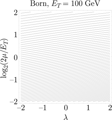
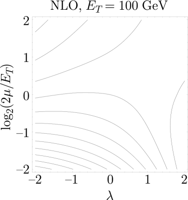
(a)	(b)

FIG. 1.: Contour plots of the Born and NLO jet cross section at $E_{T}=\mathrm{100\ GeV}$ with 1% contour lines

We first calculate the jet cross section $d\sigma/dE_{T}$ at Born level at the transverse energy $E_{T}=\mathrm{100{\ \rm GeV}}$. Fig. 1(a) shows a contour plot of the fractional difference of this computed cross section from the standard $\overline{\mathrm{MS}}$ cross section when $\lambda$ and $\mu$ are varied. The contours represent 1% changes in the cross section. The Born level cross section is very sensitive to changes in conventions; it varies by 40% from its standard value in the region shown in the plot.

In Fig. 1(b), we show the $\mu$ and $\lambda$ dependence of the cross section calculated at NLO. The NLO terms cancel out most of the convention dependence and a saddle region is observed. The maximal change from the standard cross section is only 8%. There is a rather broad region in the parameter space under consideration where the NLO cross section changes little.

In Fig. 2, we investigate how this result depends on $E_{T}$ in the range $\mathrm{50\ GeV}\leq E_{T}\leq\mathrm{400\ GeV}$. The sensitivities of both the Born cross section (not shown) and the NLO cross section to $\mu$ and $\lambda$ increase with increasing $E_{T}$. However, the Born cross section is always far more sensitive to the $\lambda$ and $\mu$ parameters than the NLO cross sections. At NLO, saddle regions are observed for all values of $E_{T}$ shown, although the saddle point is not always at the same position in the $\lambda\,\mu$ plane.

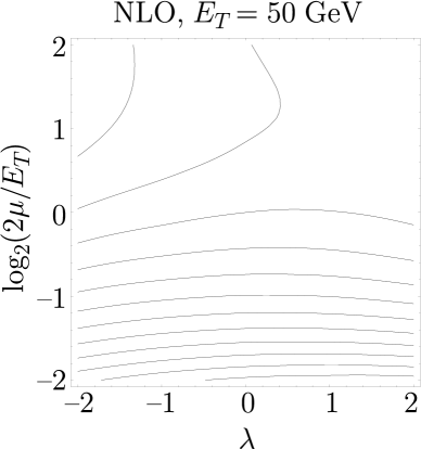
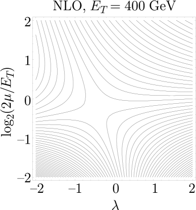
(a)	(b)

FIG. 2.: Contour plots of the NLO jet cross section at $E_{T}=\mathrm{50\ GeV}$ and $E_{T}=\mathrm{400\ GeV}$ with 1% contour lines

We can offer two comments about the results shown in Figs. 1 and 2. First, the choice $\mu=E_{T}/2$ is quite felicitous: with this choice, the dependence on $\lambda$ is almost nil. Second, there is a lot more convention dependence at $E_{T}=400{\ \rm GeV}$ than at $E_{T}=100{\ \rm GeV}$ or $E_{T}=50{\ \rm GeV}$. (One misses seeing this if one looks only at the $\mu$ dependence at $\lambda=0$. Instead, one needs to vary $\lambda$ and $\mu$ simultaneously.)

One can use the results of Figs. 1 and 2 to estimate a theoretical error to be ascribed to the calculation, as described in the introductory paragraphs. We can estimate the error as the amount by which the cross section changes when one makes a “substantial” change in $\mu$ and $\lambda$. But we need an a priori decision about what range of $\mu$ and $\lambda$ represents a substantial change. Evidently such a decision must be subjective but we cannot avoid making a choice.

Consider $\mu$ first. This parameter is supposed to represent the typical momentum that flows in loops of Feynman graphs for the process. For instance, a good guess would be $\mu=E_{T}\,\sin(R)$ where $R=0.7$ is the cone size. Thus $\mu=E_{T}/2$ is not an unreasonable guess. Clearly such an estimate cannot be good to much better than a factor of two, but our intuition is that the estimate should not be off by much more than a factor of two either. Thus we adopt a factor of two as a measure of a “substantial” scale change.

Now consider the parameter $\lambda$. The choice $\lambda=0$ represents the  MS  convention. The choice $\lambda=1$ represents the DIS convention, in which the contribution to deeply inelastic scattering from gluon initial partons is canceled by choice of convention. Since this represents a qualitative alteration in how deeply inelastic scattering appears to happen, it seems to us that $\Delta\lambda=1$ represents a “substantial” change.

We thus propose that the variation in the cross section when $\mu$ and $\lambda$ vary in the range $\{\Delta\log_{2}(\mu)=\pm 1,\Delta\lambda=\pm 1\}$ represents a minimum theoretical error in the sense that it would be a surprise (to us anyway) if the difference between the NLO result and a NNLO result were less than that. A more conservative error estimate would come from doubling the range: $\{\Delta\log_{2}(\mu)=\pm 2,\Delta\lambda=\pm 2\}$.

With this understanding, we can read error estimates off of Fig. 2. The minimum error estimate varies from 3% at $E_{T}=50{\ \rm GeV}$ to 7% at $E_{T}=400{\ \rm GeV}$. The conservative error estimate varies from 9% at $E_{T}=50{\ \rm GeV}$ to 32% at $E_{T}=400{\ \rm GeV}$.

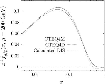
FIG. 3.: CTEQ4M, CTEQ4D and calculated gluon distribution at $\mu=\mathrm{200\ GeV}$

Klasen and Kramer have carried out an interesting investigation [4] that is in some respects similar to that reported here. They calculated the jet cross section at large $E_{T}$ using the CTEQ3D parton distributions, which are defined with the DIS convention. They compared this cross section to the cross section calculated using the CTEQ3M parton distributions, which are defined with the  MS  convention. In each case, they used the $\hat{\sigma}$ appropriate to the parton convention. They found a large difference. We agree with this result. We have calculated $d\sigma/dE_{T}$ at $E_{T}=400{\ \rm GeV}$ with $\mu=E_{T}/2$ using CTEQ4D parton distributions and the DIS version of $\hat{\sigma}$. We find that this DIS cross section is 33% greater than the corresponding  MS  cross section calculated using CTEQ4M parton distributions and the  MS  version of $\hat{\sigma}$. How can this be consistent with Fig. 2, which indicates that the DIS cross section ($\lambda=1$) differs from the  MS  cross section ($\lambda=0$) by less than 1% for $\mu=E_{T}/2$? The answer is that the DIS parton distributions obtained from the CTEQ4M distributions by using the transformation (8) are not the same as the CTEQ4D parton distributions.

We can comment in more detail. The CTEQ4D distributions are not obtained from the CTEQ4M distributions by using Eq. (8) but are instead obtained by fitting the world’s data using a DIS version of NLO theoretical formulas. In Fig. 3 we display the gluon distribution at $\mu=200{\ \rm GeV}$ as given by the CTEQ4M set, by the CTEQ4D set, and by the calculated transformation (8) from the CTEQ4M set. We see that the DIS gluon distribution calculated using Eq. (8) is negative for $x>0.5$ for $\mu=200{\ \rm GeV}$. The CTEQ4D gluon distribution is positive for all $x$. (This is a constraint imposed in the fitting procedure.) Thus the CTEQ4D gluon distribution is substantially larger at large $x$ than it might have been. This does not create a bad fit since there is essentially no data that constrains the gluon distribution at large $x$ [5]. The larger gluon distribution leads to a larger jet cross section. Thus the 33% change in the calculated cross section can be attributed to the uncertainties in fitting parton distributions, arising ultimately from the fact that the gluon distribution at large $x$ is not constrained by data.

In summary, we have investigated a two dimensional space of factorization schemes. The dependence of the jet cross section on the two parameters $\mu$ and $\lambda$ is moderate in the range $\mathrm{50\ GeV}\leq E_{T}\leq\mathrm{400{\ \rm GeV}}$. The sensitivity to $\mu$ and $\lambda$ increases as $E_{T}$ increases. Within the space investigated, the choice $\mu=E_{T}/2,\ \lambda=0$ (the  MS  scheme with a standard choice of scale) seems as good as other nearby choices. It will be interesting to see whether these conclusions change when we investigate a bigger space of factorization schemes.

REFERENCES

- [1] D. E. Soper and L. R. Surguladze, Phys. Rev. D 54, 4566 (1996).
- [2] S. D. Ellis, Z. Kunszt and D. E. Soper, Phys. Rev. D 40, 2188 (1989); Phys. Rev. Lett. 64, 2121 (1990); Z. Kunszt and D. E. Soper, Phys. Rev. D 46, 192 (1992).
- [3] G. Sterman et al., Rev. Mod. Phys. 67, 157 (1995).
- [4] M. Klasen and G. Kramer, Phys. Lett. B 386, 384 (1996).
- [5] J. Huston et al., Phys. Rev. D 58, 114034 (1998).