SLAC–PUB–8285

December 1999

Abstract

In these lectures I discuss the impact of soft hadronic physics on predictions for $B$ decays. Unfortunately our tools for calculating these effects are limited; even after the use of the best available tools the resulting theoretical uncertainties are difficult to delimit, and can obscure tests for the presence of beyond-Standard-Model physics. The first lecture reviews what tools are available, the second reviews in more detail two examples of how these tools can be used.

1 Lecture 1—Tools

1.1 What is the problem?

In these lectures I will follow the notation and definitions given by Yossi Nir in his lectures.[1] (For another excellent set of review lectures on CP Violation, including detailed references to the original literature see lectures by A. J. Buras [2]. For a recent book also covering this topic in detail see “CP Violation” by G. Branco et al. [3])

The physics of $B$ meson decays is governed by weak decay processes. Weak decays and any hard QCD effects are calculable by perturbation theory methods, but soft QCD effects not are directly calculable. Such effects are inevitably part of the meson decay process; they define the internal structure of mesons, the branching fractions to few and many-body channels, and the interactions between final-state hadrons once they have formed. Their impact can mask our ability to relate measurements to underlying Standard Model (CKM) parameters. This problem is a familiar one, it is not new in $B$ physics; in fact it is a much worse problem for lighter meson decays. The larger $B$ mass makes some of the physics more calculable, but even in the limit of extremely large $B$ mass there would be some work to do to deal with soft QCD effects.

Hard and soft QCD effects are separated by the scale of the momenta compared to the parameter $\Lambda_{QCD}$. This is the scale at which the strong coupling constant $\alpha_{s}$, as defined perturbatively, becomes infinite. Physically this scale sets the size of hadrons. Any freely propagating quark or gluon with momentum small compared to this scale is a fiction—such particles are not observed because of confinement. Said another way: in this regime QCD perturbation theory is not meaningful and nor are Feynman-type diagrams, which are after all just a short-hand for perturbative calculations. Any time you see a line in a diagram for a low-momentum quark or gluon you should be suspicious. In reality any such line comes dressed with a multitude of soft gluon emission and absorption processes, and also additional soft quarks and antiquarks. This part of QCD physics is not perturbatively calculable. To incorporate its very real effects we must resort to other tools. Conversely, for quarks or gluons with momenta large compared to the scale $\Lambda_{QCD}$ QCD perturbation theory is an effective and accurate tool.

“Hadronic effects” in my lecture title refers to the soft part of the physics. In my first lecture I will review what tools are available to treat the problem and briefly comment on the uses of these tools. For some further discussion of some of the topics that I treat rather briefly here see A. F. Falk [4]. In the second lecture I will turn to a few specific examples that illustrate in more detail how these tools can be used. Even with the best available tools some residual uncertainties about the impact of soft physics remains. The term “theoretical uncertainty” is used here to characterize impact of this poorly-calculated physics on the extraction of well-defined parameters such as the elements of the CKM matrix. One unfortunate consequence of these uncertainties is that they can mask possible new physics effects, as they obscure the relationship between the data and clean Standard Model predictions.

The goal is then to minimize the parts of the calculation affected (or should I say infected?) by these uncertainties. In addition one hopes that, eventually, comparison of data and calculations for many channels can provide some confidence in the reliability with which the residual uncertainties can be estimated. However it is important to remember that the estimates of these uncertainties are just that, estimates. They may be based on nothing more than a particular theorist’s gut feeling about the subject. The models and approximations used are often simply not well-controlled enough for one to know how big the corrections might be. It is not justifiable to treat these estimated uncertainties as if they were statistical errors. This is often done; procedures such combining these uncertainties in quadrature and quoting probabilities for a deviation of twice the theoretical error as if these were statistical standard deviations are all too common.

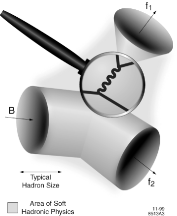
Figure 1: The hard and soft regions of a typical $B$ Decay. The shaded area contains many (undrawn) soft gluons and quark-antiquark pairs, only the hard process (within the magnifying glass) is perturbatively calculable.

Figure 1 indicates why the soft physics is usually unavoidable. We can use perturbation theory to calculate the part of the diagram within the inner magnifying lens, that is the short distance parts. The weak decay is short distance because the mass of the decaying $b$-quark is small compared to the $W$-mass, so the $W$ is highly virtual. At the same time (and here the difference with lighter mesons appears), the $b$-mass it is heavy enough that the produced quarks in general have momenta which are large compared to $\Lambda_{QCD}$. In addition hard gluons exchanged between these particles can be included perturbatively. However the initial and final hadron wave-functions, the quantities that describe these hadrons in terms of their quark content, are not perturbatively known, nor do they contain only hard quarks. Even if we take the simplest possible picture of a $B$-meson as a static heavy $b$-quark surrounded by some wave-function distribution for the light quark, that light quark has a typical momentum set by the size of the meson and hence, by definition, of order $\Lambda_{QCD}$. In most calculations of few-body decays this “spectator” quark (so-called because it does not participate in the weak decay except in the case of annihilation diagrams where it is clearly no longer a spectator), is assumed to hadronize as a valence quarks of one of the final mesons. This certainly does the book-keeping of charge etc. correctly, but it gives a deceptively simple diagrammatic picture. Such a quark cannot be included in the hard or short-distance part of the calculation; any estimates that depend on treating it as a freely propagating particle are at some level suspect.

In making the division between hard and soft physics an arbitrary and unphysical scale $\mu$ is introduced into the problem.[5] This scale must be chosen to be large compared to $\Lambda_{QCD}$ but is otherwise unconstrained. As is usual in QCD calculations one ends up with terms of the form $\alpha_{s}(\mu)ln(km_{b}/\mu)$ where k is some number (probably of order unity) and the scale $m_{b}$ enters because it is the quantity that defines the scale of momenta flowing in the hard quark lines. In order to avoid having this logarithm be large, it is convenient to choose $\mu$ of order $m_{b}$, provided that does not make $\alpha_{s}(\mu)$ too large. Here is where the $B$ system theoretical analysis is in much better shape than that for charm decays or especially for $K$-decays. The fact that $m_{b}$ is large compared to $\Lambda_{QCD}$ makes the hard/soft division a relatively clean business in $B$ physics.

In these two lectures I will confine my attention chiefly to two body (or quasi-two-body) decays, for the sake of specificity. The problem of dealing with soft hadronic physics effects is not unique to calculations of two body decays, nor are the general statements made below about methods and symmetry limits special to those decays. Many of the general approaches I mention here also have some applications for inclusive processes and for many body decays. My intent here is not to teach you to use any of the tools that I discuss, but rather to make you aware of them and of their uses, and their limitations. To actually learn to use these tools and approximation methods requires more time than we have available in these two lectures.

As was demonstrated in Yossi Nir’s lectures[1], two-body and quasi-two-body decays to states which are $CP$ eigenstates are of particular interest in neutral $B$ CP violation studies. Such states occur only for the case of two pseudoscalars, or one higher spin (typically spin 1 is studied) and one pseudoscalar, because for both these cases the decay of a spin-zero $B$ can give only one possible relative angular momentum for the two produced particles. Hence a state of definite CP is produced. For two higher spin particles, even when the particle content of the state is CP-self-conjugate, the $B$ decay produces an admixture of CP-even and CP-odd final states because both even and odd relative angular momenta between the two produced particles are allowed. In many cases such systems can be separated into states of definite CP via angular analysis of the decays of the two quasi-stable “final state” particles.[6] Then methods similar to those discussed here for the simpler modes can be applied, once sufficient data is available. Without this separation a “dilution” or cancelation effect occurs in the measured asymmetry; the CP-odd states contribute the same asymmetry as the CP-even ones except for an overall sign, so the two contributions partially cancel each other.

Methods for extracting CKM parameters from asymmetries in production of inclusive final states with a particular CP-self-conjugate quark content have been suggested.[7] These depend on estimates of the CP-even and CP-odd fractions of the decay final states. Such estimates are made at the quark level. They are reliable for the total inclusive rate because hadronization, being a strong interaction process, respects CP symmetry. Typically they suffer from large hadronic uncertainties once any cuts are introduced. Such cuts are unavoidable; they are needed either to define experimental apertures or to discriminate data from backgrounds. I will not discuss such methods further here.

1.2 Scales, Exact Limits and Expansions around them.

One of the things that makes the physics of $B$ decays complicated is that many scales can play some role in the problem. Roughly in order of increasing size these are

$$m_{u},m_{d},m_{s},\Lambda_{QCD},m_{c},m_{b},\mu$$

where the scale $\mu$ is an unphysical parameter introduced in QCD marking the division between hard and soft QCD effects calculations while $\Lambda_{QCD}$ is the scale that defines the running of the coupling in QCD.

For any significant hierarchy in these scales it is instructive to pursue the limit in which either the small scale is taken to zero, or the larger one to infinity. For example, since $\Lambda_{QCD}/m_{b}\ll 1$,and $\Lambda_{QCD}/m_{c}<1$ the heavy quark limit $m_{c}/m_{b}$ fixed, $m_{b}=\infty$ is a useful approximation to the real world. It is useful for two reasons. First the theory has additional symmetries which provide exact constraints in this limit. These constraints can be used to limit or relate various model parameters by requiring that the model have the correct limiting behavior. Second, one can calculate corrections to this limit as a power series in small quantities, namely ratios $\Lambda_{QCD}/m_{b}$ and $\Lambda_{QCD}/m_{c}$. This is called the heavy quark expansion. One has good control over the sizes of neglected corrections and hence over theoretical uncertainties due to these corrections. Unfortunately the second ratio, $\Lambda_{QCD}/m_{c}\approx 1/3$ is not so small in the real world; quantities where such terms are not suppressed have significant corrections to the limiting behavior. Cases where the leading correction is second order in this ratio are particularly attractive for this approach. Working down the scale hierarchy the following approximations and limits can be considered:

$(m_{s}-m_{d})/\Lambda_{QCD}<1$	Limit: $m_{u}=m_{d}=m_{s}$	SU(3) Invariance
$(m_{d}-m_{u})/\Lambda_{QCD}\ll 1$	Limit: $m_{u}=m_{d}$	Isospin Invariance
$m_{u}/\Lambda_{QCD}\ll 1,m_{d}/\Lambda_{QCD}\ll 1$	Limit: $m_{u}=0,m_{d}=0$	Chiral Invariance.

Each of these limits can be useful in restricting uncertainties in hadronic physics effects by introducing constrained parameterizations with somewhat controlled corrections. Examples will be discussed in more detail below, and in the second lecture. One point of caution: sometimes the interplay of more than one of these scales can limit the effectiveness of such expansions. Terms which might be treated as small because they contain inverse powers of a large mass cannot be disregarded if at the same time they contain inverse powers of a small mass.

Many of the methods for estimating matrix elements or form factors do not introduce any explicit $\mu$ dependence in them. Thus, at best, the estimates can be valid at only one value of $\mu$. Often we have no good arguments to choose that scale. It is not uncommon for theorists to characterize the uncertainty introduced by this error in matrix element calculations by looking at the variation of the result over the range from $m_{b}/2\leq\mu\leq 2m_{b}$. This choice of range has no theoretical justification. In some model calculations the natural scale for the model is a light hadron mass scale, too small a scale to be acceptable from the QCD point of view. Because of this mismatch between the scale at which the model estimate of the matrix elements can be made and the plateau region of the coefficient calculation it is difficult to characterize the size of the uncertainty in calculations that depend on such models. Methods such as lattice calculation where the matrix element calculation does have explicit scale dependence give much better hope for eventual results with well-controlled uncertainties.[8]

1.3 Heavy Quark Limit

This limit is most useful in the context of decays $B\rightarrow DX$, particularly the semi-leptonic processes; for example it provides important control over the theoretical uncertainties in the extraction of $V_{cb}$. The best cases are those where the leading correction is quadratic in the quantity $\Lambda_{QCD}/m_{c}$, since this ratio is not small enough for terms proportional to a single power of it to be a small correction. For channels with no final state charm particles one can use the heavy quark limit to relate $B$ decays to corresponding $D$ decays, for example extracting the behavior of form factors for $B$ decay from those measured in the $D$ decay case. The accuracy of this approach is limited, both by the accuracy with which the $D$ decays are measured and by $\Lambda_{QCD}/m_{c}$ corrections. There is a large literature on the subject of heavy quark limit calculations, I will not discuss these methods further here.[9]

The heavy quark limit is generally applied for hadronic $B$ decays only in combination with the factorization approximation. In the cases $DX$ it has been shown that factorization is valid in the heavy quark limit for a particular kinematic region.[10] For charmless decays the combination of the two methods adds uncontrolled theoretical uncertainties.

1.4 Isospin

Isospin analysis is a useful tool in some $B$ decays, principally for its role in separating gluon-mediated penguin contributions from tree-diagram contributions (see Yossi Nir’s lectures for definition of these two types of diagrams). The crucial point is that gluons have isospin zero which limits the isospin amplitudes to which they can contribute. The details of how the isospin information is used depends on the channel. I will review this in some further detail for a couple of channels below and in my second lecture.

For this young an audience it is probably necessary to start a discussion of isospin analysis by defining what is meant by isospin. Isospin is an SU(2) algebra in which the up and down quarks are treated as two identical members of a doublet. Note this strong interaction doublet is similar to, but not the same as, the weak SU(2) (sometimes also called weak isospin) doublet which pairs the up quark with a linear combination of down-type quarks

$$d\cos(\theta_{12})\cos(\theta_{13})+s\sin(\theta_{12})\cos(\theta_{13})+b\sin(\theta_{12})\sin(\theta_{13}).$$

Isospin is a symmetry of the strong interactions but not of electroweak, which clearly distinguish quark charges and flavors. It is also broken by quark mass terms. Historically the name isospin came about because physicists were familiar with the SU(2) algebra as the algebra of spin, and from the relationship of the multiplets of this symmetry to the isobars of nuclear physics (nuclei of equal A). From a modern perspective we can understand that hadrons form approximately degenerate isospin multiplets with mass differences small compared to the average mass of the multiplet because most hadron masses are dominated by $\Lambda_{QCD}$. The up-down quark mass difference is small on this scale, even though their mass ratio is far from 1. The exception is that pseudoscalar octet masses scale as $\sqrt{m_{q}\Lambda_{QCD}}$ and thus the effect of quark mass differences can give larger isospin breaking in this multiplet.

Isospin-breaking can also be significant in the neutral meson states. Ideally the two neutral quark-antiquark states have $I=0$ and ($I=1,I_{3}=0$): $\eta_{ud}$ and $\pi_{0}$ for the pseudoscalars, $\omega$ and $\rho$ for the vectors. In actuality, because the up and down quark masses are not identical, the mass eigenstates have small admixtures of the wrong isospin state. This can lead to important contributions that are neglected if the physical particles are treated as having a definite isospin. [11] (The notation $\eta_{ud}$ also serves to warn that, for the pseudo-scalars, the strange-antistrange combination is also mixed into the physical $\eta$ particle; $\eta_{ud}$ means that combination of $\eta$ and $\eta^{\prime}$ with no strange quark part.)

The photon and the $Z$ each couple to up and down quarks with a well-defined ratio of I=0 and I=1 couplings, for both vector and, in the case of the $Z$, axial vector couplings. These couplings are usually written in terms of coefficients $g_{1}^{X},g_{2}^{X}$ for coupling to $u$ and $d$ quarks respectively, with superscripts $X=V,A$ for the vector and axial vector couplings respectively. The combination $(g_{1}^{X}\pm g_{2}^{X})/\sqrt{2}$ are the definite isospin couplings. This relationship between coefficients gives a relationship between the amplitudes of definite isospin for a given $Z$-mediated or photon-mediated process if final state interactions are neglected. The final state interactions introduce corrections, including complex phases from absorptive parts, which are in general different in the different isospin states and cannot be calculated from first principles—that is without further assumptions.

Since photons and $Z$ bosons have $I=1$ as well as $I=0$ couplings to quark-antiquark states electroweak penguin effects cannot be removed by the same isospin analysis that eliminates QCD penguin effects. [12] Their impact varies from channel to channel, but must be considered. This limits the usefulness of isospin in removing hadronic uncertainties in the extraction of CKM parameters from CP violation in some weak decays. However in many channels the electroweak penguin effects can be shown to be small. Then the uncertainties that they induce in the extraction of CKM parameters are likewise small.

As an example of how isospin enters in $B$-decays let us consider the decays based on the quark process $b\rightarrow u\overline{u}d$. [13] These three final quarks can have either $I=1/2$ or $I=3/2$, thus we can label the quark transition as $\Delta I=1/2$ or $\Delta I=3/2$. The additional (spectator) quark (and hence the charged $B$ and $B_{d}$) are an isodoublet. Thus, combining this initial isospin with the transition isospin $\Delta I$, we find four possibilities $\Delta I=1/2,I_{f}=0$; $\Delta I=1/2,I_{f}=1$; $\Delta I=3/2,I_{f}=1$ and $\Delta I=3/2,I_{f}=2$ for these decays. The gluonic penguin can contribute only to the first two cases, because the gluon couples only to the $I=0$ combination of quarks $u\overline{u}+d\overline{d}$. Hence gluonic penguin contributions have $\Delta I=1/2$ only. Any pure $I=2$ contribution is thus unaffected by gluonic penguin contributions. Up to corrections from electroweak penguins, it has the property $\overline{A}_{2}/A_{2}=1$ in the Standard Model. Thus, if this contribution can be isolated, it can provide a relatively clean estimate of the related CKM parameter in channels where the electroweak penguin effects can be demonstrated to be small relative to the dominant terms.

Another reason to arrange the calculation in terms of isospin amplitudes is that final state interactions mix states of different charge structure but, since they are strong interaction effects, do not change isospin. Let us expand in the basis of strong interaction eigenstates $\,\left|\,{i^{I}}\right\rangle$, for which the scattering matrix is diagonal. The diagonal strong interaction scattering matrix contains an independent strong phase for each entry

$$\left\langle{j^{I}|{\cal H}|i^{I}}\right\rangle=\delta_{ij}e^{2i\delta^{I}_{i}}.$$ (1)

The eigenstates have definite isospin, but include both two-particle and many-particle components. Thus more than one eigenstate $\,\left|\,{i^{I}}\right\rangle$ exists for each isospin $I$.

The kinematic structure of each operator is different, thus the states of given isospin produced from the $B$ by two different operators are, in general, different linear combinations of the strong interaction eigenstates; we write $\left\langle{i^{I}|{\cal O}_{j}|B}\right\rangle=x^{I}_{i}({\cal O}_{j})$. The rescattering effect introduces the square root of the scattering matrix[14]; heuristically one sees this by noting that the process is not going from an in state to an out state, but starting “in the middle” from a pointlike local superposition and evolving to an out state. Finally, to consider a given two-body final state $f^{I}$ one needs the overlap $\left\langle{f^{I}|i^{I}}\right\rangle=a_{i}^{I}(f)$. Thus one can write

$$A^{I}({\cal O}_{j},f) = \Sigma_{i}<f^{I}|i^{I}>e^{i\delta^{I}_{i}}\left\langle{i^{I}|{\cal O}_{j}|B}\right\rangle$$ (2)

$$= \Sigma_{i}a^{I}_{i}(f)e^{i\delta^{I}_{i}}x^{I}_{i}({\cal O}_{j}).$$

This expression is not very useful since, in general, we cannot calculate any of the quantities in the right-hand side. However, it does serve to destroy a couple of myths that appear now and then in the literature. The first is that the only effect of rescattering is to introduce a phase in the isospin amplitudes. The second is that the strong phase for an amplitude with a given isospin is the same independent of the operator. A little playing with the above expression, say for the cases where there are just three strong eigenstates, will show that neither of these statements is true in general. One sees that they would each be true if there were only a single strong eigenstate excited for each isospin, or if the two-body state of definite isospin were by itself a strong interaction eigenstate. (In general, neither of these conditions is true.)

1.5 SU(3) Symmetry

This is another approximate strong interaction symmetry, very much like isospin except that in addition to equal mass up and down quarks the symmetry limit requires the strange quark mass to be degenerate with them. Since the ratio $(m_{s}-m_{d})/\Lambda_{QCD}$ is not so small, SU(3) breaking effects can be large. In $B$ decays the most common use of SU(3), beyond its isospin subgroup, is the application of results due to another SU(2) subgroup of the SU(3), traditionally called U-spin. U-spin treats the $s$ and $d$ quarks as a doublet of identical particles. For example, it relates rates where pions are replaced by kaons, and/or $B_{d}$ by $B_{s}$. [15]

In the factorization approximation, for any quantity where an axial current produces a pseudoscalar meson the SU(3)-breaking effect is known, it is the ratio $f_{K}/f_{\pi}$, which is measured to be $1.22\pm 0.01$. For the vector current producing a vector meson the relevant correction factor is $F_{K}/F_{\pi}$. Similar corrections occur for transition matrix elements. These corrections provide, presumably, a good first estimate of SU(3) breaking corrections, though there may be further corrections due to differences in final state scattering effects for the two different mesons. At the $B$ mass scale it is reasonable to assume that these are small corrections. However for many other contributions the use of the ratio $f_{K}/f_{\pi}$ (or $F_{K}/F_{\pi}$) to estimate the SU(3) breaking is not justified even in factorization approximation, and large theoretical uncertainties remain. In some calculations the two SU(3)-related amplitudes for these cases are allowed independently parameterized magnitudes and the SU(3) symmetry approximation is applied only to identify their strong phases. [16] Once again the corrections to this approximation are expected to be small at the $B$ mass. However I do not know how to quantify the expected size of “small” effects due to SU(3) breaking of the strong-rescattering phase relationships. In any particular case one can test the impact of relaxing this constraint by looking at how the fit for the CKM parameters of interest change with the difference between the two strong phases, but no clear statement prescription for what would be a “reasonable range” of phase differences to allow in such a treatment can be given.

1.6 Chiral Symmetry

The chiral limit and chiral perturbation theory are based on the approximation that the up and down quarks are massless in which case the pion is a Goldstone boson. This leads to an expansion of amplitudes for the production of an additional soft pion in terms of the amplitude without that pion and correction terms which occur as powers of the momentum of the soft pion scaled by $\Lambda_{QCD}$. (This scaling defines what is meant by soft in this context.) While this method has some uses in $B$ physics calculations [17] it is not a useful tool for the treatment of two body hadronic decays, since the pions produced in such decays are not soft. I will not discuss chiral expansions further in these lectures.

1.7 QCD Sum Rules

These are conditions derived from the analytic structure of QCD perturbation theory.[18] Sum rules typically relate certain matrix elements or derive constraints on their kinematic form in particular limits. Such constraints are useful in limiting the arbitrariness of models, for example those for form factors in semi-leptonic decays. The BaBar Physics Book contains an appendix which discusses this subject. I will not treat it further in these lectures.

1.8 Lattice calculation of matrix elements

Ideally we need a method for calculating the long distance contributions, that is the matrix elements, that correctly includes all soft physics. This would also give the correct sensitivity to the hard-soft division scale $\mu$. The method with the best hope of doing this is lattice calculation.[8] QCD sum rules can also be used to extract information about certain properties of form factors, but are not powerful enough to calculate the matrix elements themselves. Unfortunately, for most the cases of interest here, the same thing must be said about the lattice calculation of matrix elements, at least at the current state of the art.

For two-body $B$ decays these matrix elements are three-point functions connecting the initial $B$ to the two final-state particles. In actuality what is calculated on the lattice so far is a less-demanding two-point function, where one of the final particles has been “reduced in”.[19] It thus appears in the operator that is evaluated, rather than as a final state particle. This removes all sensitivity of the calculation to final state interaction phases, which are one of the major issues for CP-violation physics.[20] Furthermore, most of the relevant lattice calculations have so far only been made in the “quenched approximation” —which means in the approximation of suppressing any virtual quark-antiquark-loop contributions. As with experiments, lattice calculations then have a statistical uncertainty of their result and in addition non-statistical (or systematic) uncertainties arising from these various simplifying approximations. The former are readily estimated and clearly given in lattice results, the latter are hard to estimate and hence again significant theoretical uncertainties remain in most cases.

Where an unquenched calculation exists results are sometimes significantly different from unquenched results for the same quantity. We have no good understanding of how to quantify these differences prior to making the more difficult unquenched calculations. A growing number of unquenched calculations are appearing, but as yet no true three-body calculations. Again there is a large literature on this subject and I do not the time (nor the expertise) to cover it in detail.[8]

There are a number of quantities relevant to the extraction of CKM parameters from $B$ physics for which the lattice calculations are in much better shape than for the three body matrix elements discussed above. For quantities such as $F_{B}$, and many the various $B_{i}$ parameters (parameterizing the ratio of true matrix element to vacuum insertion approximation results for the QCD operators ${\cal O}_{i}$) unquenched calculations are beginning to be feasible. Reliable values (with uncertainties in the few percent range) are expected for most of these quantities within the next few years.

1.9 When are these methods useful?

I have summarized a fairly large “bag of tricks” for dealing with hadronic effects. Remembering Feynman’s dictum that if you have one good method you don’t need any others, the length of the list alone should give you an idea of the state of the problem! The applicability and efficacy of each of these methods varies from channel to channel. In the best cases we do not need any of them, because, as Yossi explained, when amplitudes with only a single weak phase dominate a decay, as is the case for the channel $J/\psi K_{S}$, the hadronic amplitudes cancel out in the ratio that defines the CP asymmetry. Then none of the uncertainties in calculating the matrix elements matter. Such a mode gives the cleanest relationship between a CKM matrix element phase and a measured asymmetry. Conversely the problems are worst when the same channel receives two comparable-magnitude contributions, say from suppressed tree diagrams and from penguin diagrams, or from two different penguin diagrams in a channel with no tree contributions, and the two contributions enter with different weak-phases, that is with different CKM matrix element coefficients. In each such case the relative strength and the relative strong phases of the two contributions affect the relationship between the measured asymmetry and any CKM parameter. One must then use whatever tools are available to try to make estimates of these effects, and equally important, to constrain the uncertainties in these estimates.

1.10 Approximations that do not come from exact limits

In many cases the methods described above are not sufficient to obtain all the desired information. When this is the case one is forced to resort to less-controlled approximations, which generally have some intuitive model as their underpinning. Such methods are very useful, for example to obtain estimates of the expected branching fraction for various channels. The most commonly used approximation is that of factorization, which I will discuss shortly. It is difficult to obtain any good estimate of the theoretical uncertainties introduced by such an approximations. Thus it is very difficult to find convincing evidence for non-Standard-Model contributions from any conflict between such estimates and measured results. However they are part of the standard toolkit for calculating $B$-decay processes and so are worth mention here.

1.11 Factorization

This approximation starts from the operator product expansion and provides an estimate of the matrix element of the local four-quark operators. One takes any such operator and finds any possible Fierz-rearrangement that groups the four quark fields into two that can create one of the final-state hadrons from a vacuum state, and two that describe a transition matrix element from the $B$ to the other final state hadron. All final state interactions between the two hadrons are ignored, as are any operators that cannot be arranged in this way. This is a very useful approximation as it allows a few-parameter model to describe many two-body decays, using transition matrix elements measured elsewhere, for example in semileptonic decays.

The idea behind this ansatz is that the region of the phase space where the two-body final state is most likely to be produced is that where two quarks that form a meson are produced moving roughly together and in a color-singlet combination. Since the operator that produces them is local, the state so made is a local color singlet state. Hence, unlike a real finite-sized hadron, it has a very small strong interaction cross section with the other quark-antiquark system. Since the two systems are rapidly moving apart, they are far separated from it before the local state has evolved into its final finite-sized configuration as a hadron. Thus it can be expected that no significant strong interaction rescattering occurs between the two mesons so formed. This “color-transparency” argument is attributed to Bjorken.[21]

When the two quarks that have the right flavor and tensor structure to form the single meson are not automatically in a color singlet state the color transparency argument is less immediately obvious. Effectively the requirement that the meson is formed projects out the color singlet part of the $\overline{q}_{\alpha}\Gamma_{i}q^{\prime\beta}$ operator (here $\Gamma_{i}$ denotes some gamma-matrix structure and $\alpha$ $\beta$ are color indices). The color counting then gives a suppression of $1/N_{c}$ since the “color-allowed” contribution

$$\Sigma_{\alpha}\left\langle{m_{1}|\overline{q}_{\alpha}\Gamma_{i}q^{\prime}|0}\right\rangle\Sigma_{\beta}\left\langle{m_{2}|\overline{q}_{\beta}\Gamma_{i}q^{\prime\beta}|B}\right\rangle\propto N_{C}^{2}$$ (3)

whereas the contribution

$$\Sigma_{\alpha}\Sigma_{\beta}\left\langle{m_{1}|\overline{q}_{\alpha}\Gamma_{i}q^{\prime\beta}|0}\right\rangle\ \left\langle{m_{2}|\overline{q}_{\beta}\Gamma_{i}q^{\prime\alpha}|B}\right\rangle\propto N_{C}\ .$$ (4)

This is the “color-suppressed” factorized contribution.

If the argument for neglecting final state interactions is rephrased in the language of strong interaction eigenstates given in the isospin section above, it looks much less attractive. As best I can see, it seems to say that the operators excite a linear combination of strong interaction eigenstates each of which gets a strong phase from rescattering, but in such a way that their vector sum is unchanged. (Another option, that looks even less plausible, is that the $B$-decay forms only a single strong interaction eigenstate involving any two pion component, and that that state has zero rescattering phase.)The general formalism instead suggests that configurations where the two quarks that make the final meson are not produced traveling together can contribute, via rescattering, to the two-body final state, even when naive expectations say that is unlikely. This contribution may indeed be small, but we cannot say how small. Our intuition rejects this possibility just because we know that for any given many-body state the probability of rescattering to two pions is typically small. However, at the $B$-mass, the cross section for two pions in an $s$-wave to scatter into many pions is not expected to be small. Thus the inverse process must also be possible for some configurations of the many particles. The problem is that any way of making the exclusive two body final state is suppressed, either because it involves a small corner of the four-quark phase space where two quarks happen to move together or because it involves a many particle to two particle rescattering. Intuition is generally a remarkably poor guide to discovering which of two unlikely events is more likely. I make this comment just to show how little we actually know—and that models can seem quite plausible in words but have little calculational basis. It is not that I know the color transparency argument is wrong—just that I know no way of proving that it is right either.

There have been a number of papers devoted to the impact of final state interactions, which are neglected in the factorization approximation. Some approach the problem generally, others consider specific channels. Some sample papers on this topic are given in the references. [22]

Recent work by Beneke, Buchalla, Neubert and Sachrajda [23] has introduced a more detailed study of how this factorization idea plays out in a one loop calculation, and at leading order in $\Lambda_{QCD}/m_{b}$ Their approach depends on certain assumptions, such as the dominance of the simple quark-antiquark state in the composition of the meson wave-function, compared to any contribution where additional soft quarks and antiquarks play a key role. It is not based on a rigorous operator product starting point, even in the infinite $m_{b}$ limit. They find that there are certain additional contributions that are ignored in the simplest factorization calculations, which means there are more input parameters to be determined in their calculations than in the usual factorization approximation calculations. However once these contributions are added they find that final state interactions are suppressed at the one loop level, because of cancelations of the type one would expect from color-transparency arguments such as that given above. They are currently in the process of extending their study to the level of two-loops.

One problem with the factorization approach is that is gives no scale dependence for the matrix elements. Since the coefficients are scale and renormalization-scheme dependent, naive factorization cannot be precisely true except possibly at some particular scale, and in conjunction with a particular choice of renormalization scheme. A common approach to this problem is to use the induced scale and scheme dependence as an estimate of the theoretical uncertainty of the method. However this is surely not a rigorous argument, firstly because the answer depends on the range of scales allowed, and secondly because it gives no estimate whatsoever of the contributions that are ignored in the factorization approximation. The best one can say is that this dependence sets a lower bound on the theoretical uncertainty. But of course what we really need is an upper rather than a lower bound on uncertainties.

1.12 Quark Hadron Duality

This set of theoretical buzz words has two basic versions—global duality and local duality. Global duality is the statement that when averaged appropriately over some range of center of mass energies the rate for a given process predicted by a quark level calculation must be the correct result for the rate at the hadron level. For certain quantities such as the ratio of the hadronic cross section to the $\mu^{+}\mu^{-}$ cross section in $e^{+}e^{-}$ scattering this can be demonstrated to follow from the analyticity structure of the propagator function $\Pi(s)$.[24]

Local duality is the same idea applied at a given center of mass energy. In $B$ decays we cannot vary the energy, it is the $B$ mass, so to relate the quark quantities we know how to calculate to the hadronic quantities we know how to measure we are forced to make this stronger assumption. There is no good justification for the truth of this assumption, nor is there any good way to estimate the size of the uncertainty it introduces. Even within the assumption of local duality there is a weaker and a stronger form. The weaker assumption is to apply duality arguments to calculate rates for a particular class of inclusive decays, the stronger assumption is to rely on details of the quark-level kinematics to predict the hadron-level properties. In fact at the end points and in resonance regions of the spectrum this last approximation must be wrong, because quark kinematics does not know about resonance widths and hadron masses, etc. As soon as one goes from a truly inclusive prediction to one that takes into account any experimental acceptance cuts the predictions tend to become dependent on this strongest form of the quark-hadron duality assumption, and the theoretical uncertainties increase accordingly.

1.13 Parameterized Amplitudes and Models

Another way that one can proceed is to introduce parameters for each diagram or each isospin amplitude. One then obtains constraints by relating the parameters describing similar contributions in different processes, via symmetries such as isospin and SU(3). Conversely one can use models to calculate the value of the parameters for each type of contribution. Here the hope is that, with enough channels studied, these parameterized amplitudes will eventually become sufficiently constrained to be predictive. The goal is that the estimates be reliable enough to make relatively definite predictions about some of the interesting quantities, and set relatively reliable constraints on the theoretical corrections to a given calculation. It is certainly true that with enough data from enough channels we can begin to get a better control. Whether that control will become good enough that we could unambiguously identify a non-Standard-Model contribution in channels where more than one amplitude contributes remains to be seen. The history of calculations of hadronic effects in $K$-decay processes, or even $D$-decays, does not give grounds for optimism. Here we are working in a very different kinematic regime and the asymptotic freedom of QCD and the heavy quark limit begin to work in our favor. Time alone will tell how well we can do.

2 Lecture 2—Examples

In this lecture I will review some examples where the tools of isospin analysis and SU(3) discussed in the previous lecture may be useful. I will also make a few comments on the impact of hadronic effects in extracting the magnitude of CKM matrix elements, such as $V_{ub}$.

2.1 Isospin analysis for $b\rightarrow u\overline{u}d$ channels

2.1.1 Two pions

In the case of two identical particles in an orbital-angular-momentum zero state (because they are two pseudoscalars coming from a $B$ decay) the set of isospin amplitudes described for this quark content in my first lecture ($\Delta I=1/2,I_{f}=0$; $\Delta I=1/2,I_{f}=1$; $\Delta I=3/2,I_{f}=1$; and $\Delta I=3/2,I_{f}=2$) is reduced. Bose statistics requires a state of even isospin, so that the overall state is even under the interchange of the two pions. Hence the $I_{f}=1$ amplitudes are all identically zero. This means only two tree amplitudes, $\Delta I=1/2,I_{f}=0$ and$\Delta I=3/2,I_{f}=2$, and only one penguin amplitude, $\Delta I=1/2,I_{f}=0$, contribute.

Gronau and London[13] showed how a measurement of rates for all three channels $B_{d}\rightarrow\pi^{+}\pi^{-}$, $B_{d}\rightarrow\pi^{0}\pi^{0}$, $B^{+}\rightarrow\pi^{+}\pi^{0}$ and their CP-conjugates, together with a time dependent asymmetry measurement for the charged pions only, can be used to isolate the weak phase of the $I_{f}=2$ contribution. In principal, this method provides a clean measurement of $\sin(2\alpha$), where $\alpha$ is the angle $\pi-\beta-\gamma$ in the unitarity triangle. Unfortunately the rates for all these channels are low,[25] and the rate for the difficult to measure $\pi^{0}\pi^{0}$ channel is expected to be even lower. It appears that the uncertainty of the measurement of this last channel will render the method impotent to obtain a precise result.[26] Put another way, for the foreseeable future the experimental uncertainty on the neutral-pion measurement will be at least as large as the theoretical uncertainty in the shift of the measured charge-channel asymmetry from the simple form sin($2\alpha$)sin($\Delta mt)$.

2.1.2 $\rho\pi$ channels and the Dalitz plot

For $B_{d}\rightarrow\rho\pi$ three channels contribute, namely the three possible charge assignments for the $\rho$ and the pion, all decaying to the same final state $\pi^{+}\pi^{-}\pi^{0}$. However, by the arguments given in the previous lecture, only two independent QCD-penguin amplitudes exist. One can take the three independent tree amplitudes to be one for each charge channel and the QCD penguin amplitudes to be one each for $I_{f}=0$ and $I_{f}=1$. (If one plans also to use charged $B$-decay amplitudes to three pions one additional tree amplitude enters; one must measure both the three-charged and the two-neutral, one charged pion final states before significant additional constraints are obtained in this way. The latter is more difficult experimentally, so I will here discuss a study involving only the neutral $B_{d}$-decays to three pions.)

Five independent amplitudes, one CKM parameter and only three channels looks a bit discouraging. However Art Snyder pointed out to me an important feature of the physics here that could be useful. In some regions of the Dalitz plot more than one of the three channels can contribute. Hence there might be information to be extracted from the interference effects in the overlap regions. Based on his suggestion we made a preliminary study of this channel and found that this is indeed the case. The number of parameters to be fitted requires a large data sample. [27] Further studies made as part of the BaBar Physics workshop confirm this conclusion, and find that, as one might expect, the inclusion of physics backgrounds from other resonances and from non-resonant $B\rightarrow 3\pi$ decays, as well as non-$B$ backgrounds make things even more difficult. However the analysis remains an intriguing if distant possibility, so I will describe a little how it works.

The amplitudes for the specific channel decays can be written

$$A^{+-} = (T^{+-}+P_{1}+P_{0})$$

$$A^{-+} = T^{-+}-P_{1}+P_{0}$$ (5)

$$A^{00} = T^{00}-P_{0}\ .$$

The assumption made in this approach is that each of the five contributing tree and penguin amplitudes for $B_{d}\rightarrow\rho\pi$ has an independent but fixed (i.e. not kinematically varying over the $\rho$ width) strong phase, along with a weak phase given by the Standard Model. The weak phase is different for the tree graph contributions and for the dominant penguin contributions. Further the weak phase of that penguin contribution cancels the weak phase of the mixing. Using the Unitarity of the CKM matrix the sub-dominant penguin contributions can be chosen to have the same weak phase as the tree amplitude; in all further discussion of phase structure these contributions are assumed to be included in the tree terms.[28] (Note however that in making numerical estimates these two types of contributions must be considered separately.)

The additional feature of this mode is that the full $B_{d}\rightarrow\pi^{+}\pi^{-}\pi^{0}$ is a sum of the three specific $\rho$-charge amplitudes. It thus contains known kinematically-varying strong phases that arise from the Breit-Wigner form of the $\rho$ resonances (more precisely stated from the $\pi\pi$ scattering phases shifts in the $\rho$ resonance region, which are parameterized by this form). Thus the amplitude for $B_{d}$ decay is given by

$$A(B_{d}\rightarrow\pi^{+}\pi^{-}\pi^{0}) = f(k^{+},k^{0})(T^{+-}+P_{1}+P_{0})$$ (6)

$$+ f(k^{-},k^{0})(T^{-+}-P_{1}+P_{0})+f(k^{+},k^{-}0)(T^{00}-P_{0})$$

where $f(k_{i},K_{j})$ is the Breit Wigner function

$$f(k_{i},k_{j}) = {cos(\theta)\over s-m_{\rho}^{2}+i\Pi(s)}$$

$$\Pi(s) = {m_{\rho}^{2}\over\sqrt{s}}\left({p\over p_{0}}\right)3\Gamma_{\rho}(m_{\rho}^{2})$$ (7)

where the $k_{i}$ are the momenta of the two pions, $s=(k_{1}+k_{2})^{2}$, and $\theta$ is the angle in the $\rho$ rest frame between $k_{1}$ and the direction opposite that of the boost from the $B$ rest frame. The function $\Pi(s)$ parameterizes the $\rho$ resonance shape. It is defined to give the correct threshold phase-space behavior and to incorporate the measured $\rho$ width, variations in the parameterization of this function are one of the sources of residual theoretical uncertainty of this analysis.

The angular dependence is that associated with the decay of a longitudinally-polarized $\rho$ meson of charge $(i+j)$ to two pions. The related amplitude for the $\overline{B}_{d}$ decay also contributes to the time-dependent rate for the decay of an initially pure $B_{d}$ or $\overline{B}_{d}$ state. Interference between the different $\rho$ bands is enhanced by the fact that the $\rho$ is longitudinally polarized and thus the cos($\theta$) form for its decay throws the events towards the corners of the Dalitz plot. This is seen in Fig. 2, which is taken from the BaBar Book and represents a simulation using amplitudes calculated from a particular model.[29]

Figure 2: The $\rho\pi$ contributions to the Dalitz plot for $B\rightarrow\pi^{+}\pi^{-}\pi^{0}$ .

The large strong phases from the resonant behavior and the interference of the different charge-channel contributions enhances the CP-violating asymmetry in the regions of the time-dependent Dalitz plot. A multiparameter maximum-likelihood fit to the broad $\rho$-band regions of the time-dependent Dalitz plot is made, with each tree and penguin amplitude parameterized by an arbitrary magnitude and strong phase, and with the weak phases as given by the Standard model. The asymmetries then depend only on one combination of weak phases, $\alpha=\pi-\beta-\gamma$ along with nine other parameters (the magnitude and strong phases of each of the five isospin amplitudes minus one irrelevant overall strong phase). In principal, provided the $\rho^{0}\pi^{0}$ contribution is large enough, this fit will allow one to extract not only a value of $\sin(2\alpha$) free of uncertainties due to penguin contributions, but also $\cos(2\alpha$), thereby removing some of the discrete ambiguities in the solution for the Unitarity triangle. In a realistic study additional parameters and assumptions must be made to parameterize non-resonant $B$ decays to three pions and also any other resonances that contribute significantly to the three-pion final state. It remains to be seen whether sufficient data can be collected to make this analysis effective when all the contributing channels and background contributions are taken into account. Certainly it will not be easy. It will require many years of data taking at a $B$ factory. Because the final state contains a $\pi^{0}$ this mode is not accessible to the current TeVatron experiments. Preliminary studies for dedicated hadron collider $B$ experiments suggest this mode may possibly be feasible for study, but further work on signal to background ratios is needed. I still hope that this mode can eventually give us a clean $\alpha$ measurement, but I recognize that the experimental challenge is significant. Some theoretical uncertainties in the value of $\alpha$ extracted in this way remain, due to the contribution of QED penguins, and also due to the assumed constant strong phases for the isospin amplitudes and the sensitivity to the $\rho$-shape. However these effects are estimated to be small. By the time this measurement is made I expect that their impact will be under much better control.

Isospin breaking effects must also be considered as a source of theoretical uncertainties when investigating these modes. The dominant correction comes from the fact that, due to isospin breaking of the quark masses, the physical $\pi^{0}$ and $\rho^{0}$ states each have a small admixture of the isospin zero quark combination. The consequence of this effect is largest in the $\pi\pi$ analysis as it reintroduces the $I_{f}=1$ amplitude that is otherwise forbidden by Bose statistics. For the $\rho\pi$ channel the impact of isospin breaking has been estimated to be small.

2.2 SU(3) in $K\pi$ and $\pi\pi$ and limits on $\gamma$

Here I will briefly describe an analysis to extract the Unitarity triangle angle $\gamma$ from the data on various channels for $B\rightarrow K\pi$ and $B\rightarrow\pi\pi$. The work I will discuss is that of Neubert and Rosner,[30] and the subsequent paper of Neubert. [31] This analysis provides an interesting example because it uses essentially the entire toolkit of methods, the Operator Product Expansion, diagrammatic classification of contributions, isospin and SU(3), and finally factorization approximation as a way to estimate SU(3) breaking corrections. However a careful selection of the quantities for which the least accurate approximations are used leads to a relatively small theoretical uncertainty for the final result. The simple rule of thumb is that the tool with large fractional uncertainty should, if possible, be restricted to determining a small part of the overall result.

The decays $B\rightarrow K\pi$ are interesting because the tree contributions $b\rightarrow su\overline{u}$ are Cabibbo suppressed. In fact it appears that the rate is dominated by the QCD penguin contributions. However, as in the $\pi\pi$ case, certain isospin channels do not have any such contribution. The quark transition $b\rightarrow u\overline{u}s$ can have $\Delta I=0,1$ and thus with the spectator quark added $I_{f}=1/2$ or $3/2$. The gluonic penguin contributes only to $\Delta I=0,I_{f}=1/2$. Here electroweak penguin contributions cannot be ignored, as they enter at approximately the same level as the Cabibbo-suppressed tree contributions, and for all isospin amplitudes. A major part of the work then comes in estimating the corrections due to electroweak penguin effects, and the uncertainty on these corrections.

The key to the analysis is to recognize that the $I_{f}=3/2$ arises only from tree diagrams and electroweak penguins. The key initial observation is that, in terms of the isospin-based amplitudes $A_{\Delta I,I_{f}}$

$$A(B^{+}\rightarrow\pi^{+}K^{0}) = A_{0,1/2}+A_{1,1/2}+A_{1,3/2}$$

$$-\sqrt{2}A(B^{+}\rightarrow\pi^{+}K^{0}) = A_{0,1/2}+A_{1,1/2}-2A_{1,3/2}\ .$$ (8)

Gluonic penguin diagrams contribute only to $A_{0,1/2}$. Neubert and Rosner define the following quantities

$$R_{*}={Br(B^{+}\rightarrow K^{0}\pi^{+})+Br(B^{-}\rightarrow\overline{K}^{0}\pi^{-})\over 2(Br(B^{0}\rightarrow K^{0}\pi^{+})+Br(\overline{B}^{0}\rightarrow K^{-}\pi^{0}))}=(1-\Delta_{*})^{2}\ .$$ (9)

One can make the weak and strong phase dependence explicit by writing

$$A(B^{+}\rightarrow K^{0}\pi^{+})=Pe^{i\phi_{P}}(e^{i\pi}+e^{i\gamma}e^{i\eta}\epsilon_{a})$$ (10)

where $\phi_{P}$ and $\eta$ are strong phases and, in terms of the diagrams,

$$P = |\lambda_{c}(P_{c}-P_{t}-1/3P_{EW,t})|$$

$$\epsilon_{a} = 7|\lambda_{u}(P_{u}-P_{c}-A)|/P\ .$$ (11)

Similarly one can write the ratio

$$-3A_{1,3/2}/P=\epsilon_{3/2}e^{\phi}_{3/2}(e^{i\gamma}+qe^{i\omega})$$ (12)

expanded so that the weak and strong phase structure of each term is made explicit. The notation is chosen so that the quantities $P$, $q$, $\epsilon_{a}$ and $\epsilon_{3/2}$ are real and all phases are explicit. Here $qe^{i\omega}$ is the ratio of electroweak penguin type contributions to the tree type contributions to $A_{3/2}$. Only the top-type diagram gives a significant electroweak penguin contribution and that enters with a coefficient $\lambda_{t}=-\lambda_{c}-\lambda_{u}$ but the $\lambda_{u}$ contribution is dropped in the above as it is too small to matter here.

I find it convenient to introduce the quantities

$$r_{3/2} = {-3A_{1,3/2}\over A(B^{+}\rightarrow K^{0}\pi^{+})}={-\epsilon_{3/2}e^{\phi_{3/2}-\phi_{P}}(e^{i\gamma}+qe^{i\omega})\over 1-e^{i\gamma}e^{i\eta}\epsilon_{a}}$$

$$\xi = {1-a(0+)\over 1+a(0+)}=\left|{A(B^{-}\rightarrow\overline{K}^{0}\pi^{-})\over A(B^{+}\rightarrow K^{0}\pi^{+})}\right|^{2}\ .$$ (13)

Then one can write

$$R_{*}^{-1}={|1+r_{3/2}|^{2}+\xi|1+\overline{r}_{3/2}|^{2}\over 1+\xi}\ .$$ (14)

In the above equations the CP-conjugated amplitudes are obtained from their CP partners by simply changing the sign of the weak phase $\gamma$ everywhere (since $e^{i\pi}=e^{-i\pi}$).

A major point of introducing all this notation is that the quantities $\epsilon_{a}$, $\epsilon_{3/2}$ and $qe^{i\omega}$ are all small, the first two because they are suppressed by the ratio $|\lambda_{u}/\lambda_{c}|$ and the last because it is a ratio of electroweak penguin to tree, albeit enhanced by the inverse CKM ratio $|\lambda_{c}/\lambda_{u}|$. Useful results can be obtained keeping only the leading effects of these quantities. Relatively large uncertainties in these quantities translate into only small uncertainties in $R_{*}$.

This statement (which is mine, not Neubert’s) is a bit of a cheat, since the sensitivity to $\gamma$ is not in the value of $R_{*}$ but in its deviation from 1, which is expected to be small for the same reason. The interest in this problem is sparked by preliminary data from CLEO which give $R_{*}=0.47\pm 0.27$. If the value of $R_{*}$ deviates significantly from 1 then the above equations can be used to put interesting constraints on the allowed range of gamma, provided we can constrain the quantities $\epsilon_{a}$, $\epsilon_{3/2}$ and $qe^{i\omega}$. The better we can constrain these parameters, the more likely we are to be able to determine whether beyond Standard Model physics is needed to explain the measurement. Further we will need some information on strong phase differences. However even generous ranges on these quantities may translate into constraints on the allowed range of gamma. So now let us pursue the question of how and how well we can calculate each of these quantities.

The quantities $qe^{i\omega}$ turns out to be cleaner than one would expect. In general two operators contribute for the tree amplitude and four for the electroweak penguin. However two of these latter four give very small contributions to this matrix element and can be neglected. The other two are Fierz-equivalent to the two tree-type operators. Furthermore only one linear combination of these two operators contributes in the SU(3) limit, the matrix element of the other must vanish. This is another application of Bose statistics, this time to the U-spin part of SU(3). Thus even though $qe^{i\omega}$ is a ratio of an electroweak penguin amplitude to a tree-type amplitude each is dominated by a single operator in the SU(3) limit. Furthermore and the two operators (for the two diagrams) are Fierz-equivalent to one-another. This means that only a single strong phase enters—the same for both these contributions, so that the ratio is fixed by the ratio of coefficients in this limit. Thus, Neubert writes $qe^{i\omega}=(1-\kappa e^{i\Delta_{3/2}})\delta_{+}$ where $\delta_{+}$ is given by the ratio of coefficients of the $I=3/2$ electroweak and tree operators that survive in the SU(3) limit and $\kappa e^{i\Delta_{3/2}}$ is the SU(3) breaking correction to this quantity. One can then estimate such corrections and the uncertainties in them. First one estimates SU(3) breaking correction $\kappa$ by calculating it in the factorization approximation. Neubert estimates this effect to be $(6\pm 6)\%$. In this approximation $\Delta_{3/2}=0$. This then gives $qe^{i\omega}\approx\delta_{EW}=(1-\kappa)\delta_{+}=0.64\pm 0.15$, where the large percentage error reflects the large theoretical uncertainties inherent in the SU(3) and factorization approximation as well as the smaller but still significant uncertainty in the evaluation of the ratio of operator coefficients that reflects small residual scale and scheme dependence of this ratio. He also includes the effect of allowing non-zero $\Delta_{3/2}$ values in this overall error estimation, noting that allowing a phase $|\Delta_{3/2}|\leq 90^{\circ}$ would yield only $|\omega|\leq 2.7^{\circ}$.

For the quantity $\epsilon_{3/2}$ one must again rely on SU(3), which relates the $B^{+}\rightarrow K\pi,I=3/2$ tree amplitude to the corresponding tree amplitude for $B^{+}\rightarrow\pi\pi,I=2$. The measured charged $B\rightarrow\pi K$ rates determines the magnitude of penguin amplitude in the denominator of epsilon, up to corrections of order $\epsilon_{a}$ which we will discuss below. Here one expects a large SU(3) correction. This is estimated again by calculating the correction in the factorization limit, taking the factorization model parameters $a_{1}^{ij}$ and $a_{2}^{ij}$ (where $ij=K\pi$ or $\pi\pi$) and the ratio $f_{K}/f_{\pi}$ from fits to data. The only model dependent part of this SU(3) correction calculation is the ratio $F(B\rightarrow K)/F(B\rightarrow\pi)$ which is 1 in the SU(3) limit. Models all agree with the range $1.1\pm 0.1$. Since this factor enters the $\epsilon_{3/2}$ factorization calculation with a relatively small coefficient, the impact of its large uncertainty on the overall correction factor is not great. Again one must assign some uncertainty to the difference between the factorization-model based estimate of the SU(3) correction and the actual SU(3) breaking effects, but it is reasonable to expect that this estimate has correctly accounted for the largest part of SU(3) breaking corrections. Including this and all the various sources of uncertainty, both theoretical and experimental, Neubert estimates about a $25\%$ uncertainty in the extracted value of $\epsilon_{3/2}$.

The remaining quantity $\epsilon_{a}$ is inherently small because it a ratio of Cabibbo-suppressed to Cabibbo-allowed terms. It would be a source of direct CP violation $\xi\neq 1$ and may eventually be constrained by measurement of the CP-asymmetry in $B^{\pm}\rightarrow K^{\pm}\pi^{0}$ decays. Another constraint comes from using SU(3) to relate these decays to the $B^{\pm}\rightarrow K^{\pm}K^{0}$ (or $\overline{K}^{0})$ decays. (For an alternate discussion of uncertainty introduced by this approach see M. Gronau and D. Pirjol [32]). Further, $\epsilon_{a}$ can be re-expressed in terms of a difference of $I=1/2$ and $I=3/2$ amplitudes that arises solely due to rescattering effects. Neubert uses all of these arguments to estimate a “reasonable” and a “conservative” (which in this context means a more generous) range for this quantity and then explores how the constraints on gamma vary as one varies $\epsilon_{a}$ over these ranges.

My point in describing this calculation is not to present the results, which you can read in Neubert’s paper, and which indeed will change with time as experimental numbers improve. What I want to show is how the tools of SU(3) limit and factorization can be combined to obtain results which are better than either tool used separately. First the SU(3) limit prediction is calculated. Then the correction to that limit is calculated using the factorization approximation. Thus the uncertainty from factorization in the result is the uncertainty in the correction to SU(3) rather than the uncertainty in the entire effect. This is clearly an improvement over a straightforward use of either uncorrected SU(3) or simple factorization estimates to calculate the entire effect.

Even when such tricks are used to the full extent available still the question remains: how big is the uncertainty in the result after all is said and done? Unfortunately the answer is never clean. But clearly the problem is much reduced if we are debating whether an effect is $6\%$ or twice as big rather than whether it is $50\%$ or twice that. The challenge to theorists is to make the sources of their uncertainties clear, and to do as honest a job as possible of constraining them. Here work remains to be done. Neubert’s paper gives an example of a serious attempt to explore such questions in a systematic way, for a particular set of decays.

2.3 Theoretical Uncertainties

In the end, whatever the estimates might be, it is important to remember that theoretical uncertainty is not statistical; it is simply wrong to talk about the probabilities of certain results as if these estimates were in fact gaussian-based standard deviations. It is also very misleading to combine different sources of theoretical error by adding them in quadrature, though one sees this done frequently in the literature.

A false division between theoretical uncertainties and systematic errors in an experimental value is often made—at least in the minds of theorists making the initial predictions. A theorist makes a clean prediction with small theoretical errors for a quantity—say, for example, the CP-violating asymmetry in inclusive $b\rightarrow u\overline{u}d$ decays. The theorist is happy. However that quantity is in fact impossible to measure, since any real experiment has aperture limitations and in addition must apply cuts to separate the signal from background, in the example above both that from sources other than $B$-decays and that from the dominant $b\rightarrow c\overline{q}q^{\prime}$ decays. The impact of these cuts on the relationship of the measurement to the prediction must be evaluated based on some theoretical models. This is where the large theoretical errors will typically appear.

Experimentalists now often quote their uncertainties by separating out such effects as theoretical uncertainties rather than by including them in the overall systematic uncertainties. My point here is that the magnitude of this theoretical uncertainty typically will have nothing to do with the magnitude of the theoretical uncertainty for this measurement given in the original theoretical predictions. Such experiment-dependent theoretical uncertainties belong neither to the domain of pure theory nor to the domain of experiment, but live at the interface between them. They do, however, suffer the usual disease of theoretical errors—they are not statistical effects. It would be very helpful if theorists making their clean predictions could at least consider and briefly discuss what impact experimental cuts will have on the validity of their prediction. I do not mean the theorist should define specific cuts, but rather should discuss the question of whether the result can survive any cuts at all without serious degradation.

My remarks above are borne out in a well-known way in the case of the extraction of the magnitude of the CKM-parameter $V_{ub}$ from semileptonic $B$-decay data. Two general classes of methods are in the market—one uses exclusive decays and has obvious theoretical uncertainties related to the form factors (that is the QCD matrix elements) that govern the particular decay in question. The other uses inclusive semi-leptonic decays and is thus at first sight very clean. But the experiment must make cuts to remove the $b\rightarrow cl\nu$ backgrounds. The prediction for the cut data sample has comparable theoretical uncertainties to the exclusive decay cases. Eventually we need to explore both kinds of methods, since the theoretical uncertainties for the two approaches are essentially different.

Recently new predictions for extracting this same parameter from hadronic measurements have appeared. Again one group of theorists advocates an inclusive approach, and others advocate certain exclusive channels. Both are interesting; both will probably have significant theoretical errors once the real experimental limitations on the inclusive methods are understood.

In all these cases, whether semi-leptonic or hadronic decays are considered, one cannot use any of the more rigorous tools discussed above to estimate the theoretical uncertainties introduced due to experimental cuts or those due to form-factor estimates. One is forced to resort to models. Often the models work at the quark rather than the hadron level and then apply the notion of quark-hadron duality which is the assumption that the two-body hadron kinematics reflects the underlying quark kinematics. This is called “local quark-hadron duality”. It is not a justifiable assumption.

Estimates of theoretical errors in such cases tend to be very subjective. There really is no clean way to obtain them. The most common method is to try a few models and take the range of the results as the range of theoretical uncertainties. This is risky, since all the models on the market may contain the same unjustified assumption (for example that a particular form factor can be parameterized as a simple pole). Nonetheless it is common practice and perhaps the best we can do. My advice is one should simply be aware when this is the nature of the theoretical error estimate and treat the resulting numbers with a sufficient amount of salt. The recent history of statements about errors in estimates of $\epsilon^{\prime}/\epsilon$ should be a clear object lesson to experimenters on the reliability of theoretical error estimates.

References

- [1] Y. Nir Lectures, Lectures at SLAC Summer Institute (1999), in this volume.
- [2] A. J. Buras, Lectures at Lake Louise Winter Institute Feb. 1999, hep-ph/9905437 (1999).
- [3] G. Branco, L. Lavoura and J. Silva “CP Violation”, Oxford University Press (1999).
- [4] A. F. Falk, Chapter 2 of ‘The BaBar Physics Book: Physics at an Asymmetric Factory’, (SLAC report SLAC-R-504), hep-ph/9812217.
- [5] K.G. Wilson, Phys. Rev. 179, 1499 (1969).
- [6] J. R. Dell’Aquila and C.A. Nelson, Phys. Rev. D33, 101 (1986); B. Kayser et al., Phys. Lett. B237, 3339 (1990); I. Dunietz et al., Phys. Rev. D43, 2193 (1991).
- [7] M. Beneke, G. Buchalla, and I. Dunietz, Phys. Lett. B393, 123 (1997).
- [8] S. Aoki, Talk at 22nd International Lepton Photon Conference, Stanford August (1999); Stephen R. Sharpe, Talk at 29th ICHEP 98, Vancouver, Canada, 23-29 Jul 1998, hep-lat/9811006.
- [9] M. Neubert, Talk HEP 97, Jerusalem, Israel (1997), hep-ph/9801269.
- [10] M. J. Dugan and B. Grinstein, Phys. Lett. B255, 583 (1991); J. F. Donoghue and A. A. Petrov, Phys. Lett. B393, 149 (1996).
- [11] For the effects of isospin breaking in decays see, for example, S. Gardner hep-ph/9809479; hep-ph/9906269.
- [12] R. Fleischer, Z. Phys. C62, 81 (1994); M. Gronau, O. F. Hernandez, D. London, J. L. Rosner, Phys. Rev. D52, 6374 (1995); A. J. Buras, R. Fleischer, Phys. Lett. B365, 390 (1996), R. Fleischer, Phys. Lett. B365, 399 (1996).
- [13] M. Gronau and D. London, Phys. Rev. Lett. 65, 3381 (1990).
- [14] K. M. Watson, Phys. Rev. 88, 1163 (1952); R. N. Cahn and M. Suzuki, hep-ph/9708208 (1997); M. Suzuki and L. Wolfenstein , Phys. Rev. D60, 074019 (1999).
- [15] See, for example, M. Gronau, J. L. Rosner, and D. London, Phys. Rev. Lett. 73, 21 (1994); M. Gronau, O. F. Hernandez, D. London, and J. L. Rosner, Phys. Rev. D50, 4529 (1994).
- [16] M. Gronau and J. L. Rosner, Phys. Rev. Lett. 76, 1200 (1996).
- [17] For example, see M. B. Wise, Phys. Rev. D45, 2188 (1992); G. Burdman and J. F. Donoghue, Phys. Lett. B280, 287 (1992); H.-Y. Cheng, C.-Y. Cheung, W. Dimm, G.-L. Lin , Y.C. Lin, T.-M. Yan, H.-L. Yu, Phys. Rev. D48, 3204 (1993).
- [18] M. A. Shiftman, A. I. Vainshtein, V. I. Zakharov, Nucl. Phys. B147, 385 (1979); L. J. Reinders, H. Rubinstein and S. Yazaki, Physics Reports 127, 1 (1985); P. Ball, V. M. Braun Phys. Rev. D55, 5561 (1997); BaBar Physics Book, Appendix D, SLAC Report 504 (1998); P. Ball, V. M. Braun, Phys. Rev. D58, 094016 (1998).
- [19] H. Lehmann K. Symanzik and W. Zimmerman, Nuovo Cimento 1, 1425 (1955).
- [20] S. Sharpe, private communication.
- [21] J. D. Bjorken Nucl. Phys. Proc. Suppl. 11, 325 (1989).
- [22] J. F. Donoghue, hep-ph/9607352 (1996); M. Gronau , J. L. Rosner, Phys. Lett. B439, 171 (1998); M. Gronau, J. L. Rosner Phys. Rev. D58, 113005 (1998); A. F. Falk, A. L. Kagan, Y. Nir, A. A. Petrov, Phys. Rev. D57, 4290 (1998); A. F. Falk, Talk at QCD 98, hep-ph/9806538; Alexey A. Petrov, Talk at Kaon 99, hep-ph/9909312.
- [23] M. Beneke, G. Buchalla, M. Neubert, C. T. Sachrajda, Phys. Rev. Lett. 83, 1914 (1999).
- [24] E. Poggio, H. Quinn and S. Weinberg, Phys. Rev D13, 1958 (1976).
- [25] CLEO Conference Report 99-14, Y. Kwon et al., see www.lns.cornell.edu/public/CONF/1999.
- [26] BaBar Physics Book, SLAC Report 504 (1998), Paul Harrison and Helen Quinn editors, Chapter 6.
- [27] H. R. Quinn and A. E. Snyder, Phys. Rev. D48, 2139 (1993).
- [28] H. Quinn in Review of Particle Physics, European Physical Journal C, Volume 3 1-4, p. 558 (1998).
- [29] J. Charles, Phys. Rev. D59, 054007 (1999).
- [30] Matthias Neubert and Jonathan L. Rosner, Phys. Lett. B441, 403 (1998); Matthias Neubert and Jonathan L. Rosner, Phys. Rev. Lett. 81, 5076 (1998).
- [31] Matthias Neubert , SLAC-PUB-8122, to be published in the Proceedings of 17th International Workshop on Weak Interactions and Neutrinos (WIN 99), Cape Town, South Africa, 24-30 Jan 1999, hep-ph/9904321.
- [32] Michael Gronau and Dan Pirjol, CLNS-99-1604 (1999), hep-ph/9902482.