Instanton effective action formalism for 2-point and 4-point functions
Abstract
We provide an instanton effective action formalism in terms of which one can investigate the nonperturbative generation of 2-point and 4-point functions.
I Introduction
To understand the physics above the electroweak scale one needs to understand nonperturbative dynamics. If Nature turns out to be supersymmetric not far above the electroweak scale then one seems to require nonperturbative dynamics to understand how supersymmetry breaks. Otherwise, a process of dynamical symmetry breaking is required to avoid unnatural fine tuning.
An important feature of nonperturbative dynamics, is the formation of composite order parameters – fermion n-point functions that are generated nonperturbatively through strong dynamics. Much work has been done on 2-point functions because of the role they play in chiral symmetry breaking, which is not only relevant to QCD, but also to physics beyond the standard model.
Recently [1, 2] it was pointed out that 4-point functions may play an important role in flavor scale physics, high above the electroweak scale. The argument is as follows. The situation at such high scales is that fermions are (effectively) massless so that a chiral symmetry exists. Above the electroweak scale there would not be any 2-point functions that involve fermions with electroweak quantum numbers, because these would break the electroweak symmetry. The same applies to any other n-point function that breaks the electroweak symmetry. There are however some 4-point functions involving fermions with electroweak quantum numbers that are allowed at scales above the electroweak scale. One can distinguish five such 4-point functions on the basis of the chiralities of their external lines: three are chirality preserving and two are chirality changing. The chirality preserving 4-point functions can obviously respect any chiral symmetry. The chirality changing 4-point functions can be invariant under a chiral isospin symmetry, which may contain the of the electroweak symmetry, but these 4-point functions break larger chiral symmetries. If it can be generated nonperturbatively, such a 4-point function would signal the following breaking pattern
| (1) |
(The subscript indicates a vectorial symmetry.) Hence, these chirality changing 4-point functions act as order parameters for this partial breaking of chiral symmetries, which may occur at scales high above the electroweak scale. (Note that all fermions transform nontrivially under chiral isospin, which implies that masses are not allowed.)
The significance of this is that the partial chiral symmetry breaking gives a new scale high above the electroweak scale. The surviving chiral isospin symmetry can contain the of the electroweak symmetry, which means that this mechanism can exist for standard model fermions. It is therefore not necessary to introduce new non-standard model fermions to produce flavor scale physics. As a result dynamical models may become simpler.
For 4-point functions to act as order parameters they must appear at higher scales than 2-point functions do. One can imagine that for certain combinations of number of colors, , and number of flavors, , the critical coupling for the formation of 2-point functions may be higher than the critical coupling for the formation of 4-point functions. In an asymptotically free theory the 4-point functions would then be formed at a higher scale than the 2-point functions. The separation between these scale may be larger for large numbers of flavors than it would be in QCD-like theories where the coupling runs relatively quickly. Under these circumstances one would have the breaking pattern of (1) at the higher scale where the 4-point functions form and lower down, when 2-point functions form, the chiral isospin symmetry would break to a vectorial isospin symmetry. In some cases, for large enough numbers of flavors, an infrared fixed point may prevent the coupling from reaching the critical value for the formation of 2-point functions. All this is of course still speculation. The question therefore is, under what circumstances ( and ), if any, would a nonperturbatively generated 4-point function appear at higher scales than 2-point functions do?
One can start by assuming that the favorable situation exists for 4-point functions to form at a much higher scale than 2-point functions. This means that one can assume that fermions remain massless. It allows one to formulate an effective action for these 4-point functions, making the chiralities of the fermions explicit. Thus one can distinguish the above mentioned five different 4-point functions. Such an analysis was done in [2], considering only gauge exchanges. The outcome was that in the limit of a large number of colors, none of the five 4-point functions can be generated nonperturbatively. Since the analysis in [2] excluded instanton dynamics, the question naturally arises whether 4-point functions can perhaps be generated through instanton dynamics.
The instanton [3, 4] is an important nonperturbative effect that appears in non-Abelian gauge theories. The relevence of instantons in the formation of 2-point functions and, by implication, in chiral symmetry breaking has been realized long ago [5, 6]. Subsequently many authors elucidated various aspects of this mechanism for chiral symmetry breaking. For reviews see [7, 8].
Unlike the 2-point function case, calculations of the nonperturbative generation of 4-point functions through instantons has received very little if any attention so far. At present there does not seem to exist a formalism in which one can treat this problem. Therefore the purpose of this paper is to provide an effective action formalism for the calculation of the instanton contribution to the formation of 4-point functions. Because such a formalism requires as part of its derivation a consistent treatment of 2-point functions, it also provides the means to calculate the instanton contribution to their formation. Our formalism provides a consistent framework for deriving the gap equations of the relevant n-point functions through the stationarity of the effective action. The instanton contributions to the effective action are represented as diagrams that are generated from Feynman rules. These rules include a nonlocal instanton vertex for the fermion zeromodes and a fermion propagator. The nonlocal instanton vertex differs from the usual effective ’t Hooft vertex [4] in the sense that, unlike the latter, it is valid at distance scales smaller than the instanton size.
The coupling strengths in our diagrammatic language are given by: the sizes of the n-point functions and the coefficient of the instanton vertex, which depends on the gauge coupling, number of colors and number of flavors in a complicated way. For a specific size of the coefficient of the instanton vertex, the sizes of the actual n-point functions determine whether the expansion in terms of diagrams converges. Given a specific instanton coefficient, one can assume that there is some maximum size for the n-point functions for which the expansion still converges. If the actual global minimum of the effective action lies beyond the point where the n-point function reaches this maximum size, the usefulness of this formalism would be limited. However, in the case of a continuous phase transition the n-point function would have a sufficiently small value in the interesting region near the transition.
A semi-classical approximation is made to the action from which the effective action is derived. This implies that the theory behaves like a free theory apart from the presence of a background gauge field. In addition it is assumed that the instanton ensemble is fairly dilute – the average size of the instantons, , is smaller than the average separation between them, . On the basis of this diluteness we drop terms in our derivation that would be suppressed by factors of the average size over the average separation . As a result our derivation does not contain interference between zero and non-zeromodes; the overall non-zeromode determinant factorizes into non-zeromode determinants for each instanton; and the classical instanton gauge interactions fall away. The instanton vertex for the fermion zeromodes captures the important dynamics, therefore these effects are of secondary importance.
The derivation is presented in the following steps. We start in Section II by introducing the necessary source terms in the action, providing some definitions of the various functionals and defining our notation. The first part of the derivation, Section III, explains how the fermion fields are treated. An important part of this involves the treatment of the zeromodes. The result of this part is a fermion modal propagator and a nonlocal fermion vertex for the zeromodes. The next part, concerning the gauge fields, is presented in Section IV. Once all the quantum fields are integrated out one is left with an expression that can be interpreted in terms of Feynman diagrams. The relevant Feynman rules are discussed in Section V. The derivation of the effective actions then follows in Section VI. It utilizes the procedures of De Dominicis and Martin [9]. In Section VI A we derive the effective action for 2-point functions and compare it to the CJT effective action [10]. Then in Section VI B, starting with the 2-point effective action and setting the mass part of the full propagator equal to zero, we discuss the derivation of the effective action for the 4-point functions. This complicated derivation is in essence identical to the one that is provided in [2] and its details are therefore not repeated here. We conclude with a few important remarks in Section VII.
II Notation
We are considering the instanton-induced formation of fermion 2-point and 4-point functions in an gauge theory with massless (Dirac) fermions in the fundamental representation. In the semi-classical approximation we expand the action around the classical background field configurations, :
| (2) |
where denotes the “quantum” gauge field. The gauge coupling is incorporated into the gauge field and appears explicitly in the gauge kinetic term. All terms in the action with more than two quantum fields (gauge, ghost or fermion fields) are dropped. In the resulting semi-classical action , the quantum fields only interact with the background configuration but not with each other.
For the purpose of investigating the formation of 2-point and 4-point functions, we introduce the following nonlocal 2-fermion source term
| (3) |
and nonlocal 4-fermion source term
| (4) |
The implicit color and flavor indices are contracted on the sources in (3) and (4). In the diagrammatic formalism developed here, these nonlocal sources are treated as 2-fermion and 4-fermion vertices respectively. We also have the usual local source terms for the fermion fields:
| (5) |
The partition functional and generating functional are defined (in Euclidean space) as
| (6) |
Here, is the functional measure over all the fields in the action, and the Euclidean action is
| (7) |
The 2-point function is formally given by
| (8) |
while the 4-point function is
| (9) |
We perform the Legendre transformation in two steps. The first step gives an effective action for 2-point functions, , in the presence of the nonlocal source, . The second gives the complete effective action for 2-point and 4-point functions, . We are however only interested in the case where fermions remain massless. Therefore we fix the full propagator to be massless and denote the resulting effective action for 4-point functions by in terms of the amputated 4-point functions, .
In order to simplify our expressions we replace the fermion fields in the nonlocal source terms by functional derivatives with respect to the local sources, using the shorthand
| (10) |
Then these terms are pulled out of the functional integral:
| (11) |
The derivation is presented using the partition functional without the nonlocal sources,
| (12) |
up to the point where the nonlocal sources start to play a role.
III Fermion zeromodes
We first consider the fermion fields. One can split the action into a fermion part and a pure gauge part that contains no fermion fields:
| (13) |
The fermion terms in the Lagrangian in are
| (14) |
where the Dirac operator,
| (15) |
contains only the background gauge field, .
In the presence of instantons (i.e. when the background gauge field has a nontrivial winding number) the Dirac operator possesses fermion zeromodes. It is singular and cannot be inverted. One can avoid this problem by performing a projection onto the subspace of non-zeromodes and inverting the operator on this subspace only. For one instanton with massless fermions there are zeromodes. Considering a specific configuration (size, position and color orientation) of this instanton, one can separate the subspace spanned by the zeromodes from the rest which makes up the non-zeromodes. The Dirac operator annihilates the zeromodes, therefore we have
| (16) | |||||
| (17) |
where the operator projects onto the non-zeromodes, while is the projection operator onto the zeromodes; furthermore , , , , etc.
For several instantons and anti-instantons the would-be zeromodes of each one are not necessarily zeromodes of the total configuration. In fact the would-be zeromodes mix and give a spectrum of eigenvalues around zero. In our approach we keep all the would-be zeromodes separate from the rest of the fermion modes. In what follows we shall proceed to call them ‘zeromodes’ even though they are not always actual zeromodes of the total configuration.
Now we define the zeromode and non-zeromode subspaces for any specific background configuration with multiple instantons. The zeromodes of all the instantons and anti-instantons span a subspace of the space of all fermion fields. We separate this subspace and refer to it as the space of all zeromodes. The remaining part is called the space of all non-zeromodes. Note that the splitting of the space of fermion fields into zeromodes and non-zeromodes depends on the background configuration.
For ensembles of instantons and anti-instantons the Dirac operator gives a small but nonzero overlap between the zeromodes of neighboring instantons and anti-instantons. Therefore, for instanton ensembles we have, in addition to the terms in (17), the terms
| (18) |
where the superscripts and indicate that the zeromode belongs respectively to an instanton or an anti-instanton.
The cross terms of (18) are responsible for the dynamics that produce the delocalization of the fermion wave function when chiral symmetry breaking occurs. It thus plays a crucial role in the nonperturbative formation of fermion n-point functions through instantons. Without the cross terms there would be no fermion interconnection between instantons and anti-instantons other than through the interference between zeromodes and non-zeromodes via the Dirac operator.
These interference terms,
| (19) |
give contributions to the fermion propagator that mix zeromodes and non-zeromodes. However, to leading order in ( is the average instanton separation and is the average instanton size) the non-singular part of the fermion propagator does not have terms that connect zeromodes to non-zeromodes [11]. This is related to the fact that, to leading order in , the complete fermion determinant factorizes into a zeromode part and a non-zeromode part [11, 12].
Our aim is now to find a way to invert the Dirac operator, and arrive at propagators that correspond to the various types of fermion modes, while avoiding the singularities. The remainder of this section addresses this issue.
According to the preceding discussion one can express the partition functional of (12) as
| (21) | |||||
Here, is the functional measure over the fermion fields and is the functional measure over the gauge fields (quantum plus background) and the ghost fields. Using and , we pulled the cross terms of (18) out of the functional integral over fermion fields and represented them as one cross term. It must remain under the gauge functional integral because it still depends on the background gauge fields through the Dirac operator in (15).
Integrating over the non-zeromodes, we find
| (23) | |||||
where is the measure over the fermion zeromodes and is the determinant of the part of the Dirac operator associated with non-zeromodes, calculated on the subspace of non-zeromodes. The non-zeromode propagator is defined by
| (24) |
The next step is to perform the integration over the fermion zeromodes. Consider first the case of only one instanton. At the end we shall generalize the result to multiple instantons. We write the two zeromode terms in the exponent in (23) as a sum over flavors,
| (25) |
where are Grassmann variables for the zeromodes and denote c-number spacetime functions of the fermion zeromodes. For an explicit form of these functions see [6].
Performing the functional integral over zeromodes, we get
| (26) |
where denotes the functional measure over the Grassmann variables of the fermion zeromodes. The subscripts on the brackets indicate that the enclosed sources, Grassmann variables and zeromode functions are all associated with the same flavor. The result is an object that, from a diagrammatic point of view, behaves like an n-point propagator ().
It would be more convenient to turn this n-point function into an n-fermion vertex. We achieve this by adding the following source terms to the Euclidean action in (7):
| (27) |
Here each zeromode source has associated with it a new source, , and similarly an is associated to . (Integrations over the relevant spacetime coordinates are understood.)
The addition of these terms is strictly formal. The two types of sources serve merely as variables with respect to which the functional derivatives are taken. In essence, both types of sources are associated with zeromodes and are in that respect not different. However, the way they appear in the expression implies that their dynamics are different. The introduction of these source terms changes the partition functional. So now we define a new partition functional which includes these sources. Upon setting we recover .
The idea is now to amputate the n-point propagator by writing
| (28) |
Here we use the functional derivatives and . The subscripts on the right-hand side indicate that both the functional derivatives and the zeromode functions inside the brackets are associated with the same flavor.
So now we have
| (30) | |||||
The generalization of (30) for multiple instantons and anti-instantons is straightforward. The only difference is that the number of zeromodes increases. When the background configuration contains instantons and anti-instantons the product of all zeromodes in (30) runs over instead of factors.
Now we allow the cross term,
| (31) |
to operate on the propagators
| (32) |
The vertex, , connects zeromodes of instantons to anti-instantons while the bare propagator, , is associated with zeromodes of a specific instanton or anti-instanton. One can use the vertex to get a propagator that connects the zeromodes of different instantons:
| (33) |
Here propagates zeromodes between instantons and anti-instantons (the negative sign is due to the Grassmann nature of the sources). The bare propagator connects zeromodes between instantons and source vertices.
In order to simplify the notation we combine all the propagators into one,
| (34) |
and call it () the modal propagator. Its various parts, as shown in (34), depend on the background configuration in a complicated way. However, the expressions for these parts are known [11, 12, 13].
The resulting expression of the partition functional is
| (35) |
where denotes the total number of zeromodes.
We have now completed the derivation of the fermion propagator. All fermion fields have been successfully integrated out and we have a single propagator for the fermion fields. In addition we have a nonlocal -fermion vertex that describes the interactions of fermion zeromodes.
IV Gauge fields
At this point the only remaining quantum fields are the ghost and gauge boson fields that appear in the gauge action . In the semi-classical approximation the functional measure can be split into a functional measure over the remaining quantum fields, , and the measure over the collective coordinates (CC’s) that specify the background field configuration. We denote the collective coordinates by .
To evaluate the functional integral over the quantum fields, we split the gauge action into two parts: . Here consists of the kinetic terms for the ghosts and gauge bosons and the sum of the classical actions of the individual instantons. The functional integral of the part containing leads to the ’t Hooft amplitude without fermions [4]. The part of the gauge action, , that contains mixtures of different instantons and anti-instantons behaves like an interaction terms and is therefore denoted by . The latter contains no quantum fields. After integrating over the color orientations of the instantons the surviving part of is of [14]. We therefore drop from our analysis.
The fermion contribution in the ’t Hooft amplitude can be separated into a zeromode and a non-zeromode part. The non-zeromode part comes from the non-zeromode determinant which first appeared in (23). For fermions with mass , the zeromodes give a factor of , where is the renormalization scale. In the case of massless fermions, one needs additional fermion dynamics in the theory to take care of the zeromodes. Without this additional dynamics the instanton amplitude for massless fermions would vanish. In our case this dynamics is provided by the nonlocal sources or, in the effective action language, by the n-point functions.
To leading order in the non-zeromode part of the fermion determinant factorizes into separate non-zeromode determinants for each instanton [11, 12]. For instantons and anti-instantons we have:
| (36) |
where denotes a Dirac operator with only one instanton in the background field configuration.
We shall first discuss the integration over quantum gauge fields for one instanton and then at the end generalize the result for multiple instantons. Apart from the fermion dynamics that must account for the fermion zeromodes, the ’t Hooft vacuum-to-vacuum tunneling amplitude for one instanton is given by
| (37) |
where is the product of the same determinant and gauge functional integral evaluated in the absence of any instantons. Hence is a collective coordinate independent normalization constant.
The vacuum-to-vacuum tunneling amplitude in (37) becomes [4]
| (38) |
where the dependence on the gauge coupling is contained in
| (39) |
Here is the renormalization scale and . The running of the coupling in (38) is determined by . As such it gives one-loop running for the coupling that appears in the exponent in . The expression can be extended to higher orders which would cause the coupling in the monomial-part of to run as well. The prefactor in (38) is
| (40) |
with , to one loop in MS-bar [15]. Here includes a color volume factor that comes from the integral over all color orientations. This integral only gives the volume of the relevant factor group, , where is the subgroup that leaves the instantons invariant. This prefactor does not include the effect of the gauge dependence in the remaining dynamics. The complete integral over color orientations can be seen as a product of a color volume factor and an averaging over the gauge structure of the remaining dynamics. The latter, which we consider next, gives a tensor structure that indicates how color indices are contracted.
The gauge dependence of the remaining dynamics appears in the color orientation of the fermion zeromodes. One can represent this as
| (41) |
where and are gauge transformations operating on the zeromode functions to give all possible color orientations. The integral over all color orientations can therefore be written as
| (42) |
where is the Haar measure for the gauge group in which the SU(2) group of the instanton is embedded. The result of the integral in (42) for an arbitrary number of flavors, , is quite complicated. However, it simplifies significantly in the case of a large number of colors, , when one neglects the terms that are subleading in . The result is
| (43) |
where the and -indices are permutated together. Permuting the flavor indices instead of color indices, one finds that if such a permutation is odd the term receives a negative sign due to the Grassmann nature of the functional derivatives. The flavor permutations therefore lead to an antisymmetric -tensor:
| (44) |
Here is the number of flavors. The first index on each zeromode or derivative is a flavor index and the second one is a color index. Note that the flavors of the first bilinears are just those produced by the index of the product, while those on the second bilinears are contracted with the -tensor, and thus give a permuted version of the flavors on the first bilinears. One can see that for only two flavors this expression resembles the first term of the ’t Hooft vertex in [4].
We now write (35) for the one instanton case as
| (45) |
where the object plays the role of a nonlocal vertex:
| (46) |
with . A similar expression exists for anti-instantons, which we denote by . The only difference is that the zeromode functions, and , have the opposite helicities.
The quantum gauge and ghost fields interact with one instanton at a time. For this reason, when we generalize to configurations with many instantons, we get a factor of for each instanton. There is a or , for each respective instanton and anti-instanton in the background configuration. At the same time each instanton comes with a complete set of collective coordinates.
The resulting expression is
| (47) |
where each and introduces its own integral over its associated collective coordinates. The understanding is that is part of the integrand of the overall collective coordinate integral.
We now recover the original partition functional with the nonlocal sources using
| (48) |
V A diagrammatic language
In [2, 9, 10] the diagrammatic language of the underlying gauge theory was exploited to express the effective action as a functional of the relevant n-point functions. For instanton physics the necessary diagrammatic language is provided by the Feynman rules that can be derived from the expressions for in (47) and (48). These include rules for:
-
the 2-fermion and 4-fermion sources, and , that are represented by nonlocal 2-fermion and 4-fermion vertices in the diagrams;
-
the nonlocal -point instanton vertices, and ;
-
the modal propagator , represented by fermion lines, and
-
an integral over the collective coordinates of all the instantons involved in the diagram.
According to these rules is the sum of all vacuum diagrams in the presence of the collective coordinate independent nonlocal sources and . The modal propagator depends on all the collective coordinates of the background configuration. As a result disconneted diagrams do not factorize. However, if one assumes that the instanton ensemble is fairly dilute, the overall collective coordinate integral can be separated into a product of integrals – one for each connected part of the diagram. This is because the modal propagator depends only weakly on the collective coordinates of far away instantons. Under the above assumption each connected diagram only depends on the instantons that are directly involved, so that exponentiates. Therefore consists of the sum of all (collective coordinate integrated) connected vacuum diagrams.
VI The effective actions
The effective action is the Legendre transform of the sum of all connected vacuum diagrams with respect to the nonlocal sources. The Legendre transform formally replaces the dependence on these sources by a dependence on the n-point functions. However, to find the explicit expressions one must perform a resummation of the vacuum diagrams in terms of the n-point functions. This resummation hides the sources inside the n-point functions except in the term that is explicitly removed by the Legendre transform. Thus it leads to an expression for the effective action in terms of these n-point functions.
De Dominicis and Martin [9] provided diagrammatic procedures for the systematic resummation of vacuum diagrams in terms of the relevant n-point functions (up to 4-point functions). We use these procedures to derive the effective actions for 2-point and 4-point functions. While in the 2-point case we allow chirality breaking structures that can generate dynamical masses, in the 4-point case we specialize to situations in which unbroken chiral symmetries protect fermions from acquiring masses.
A The 2-point effective action
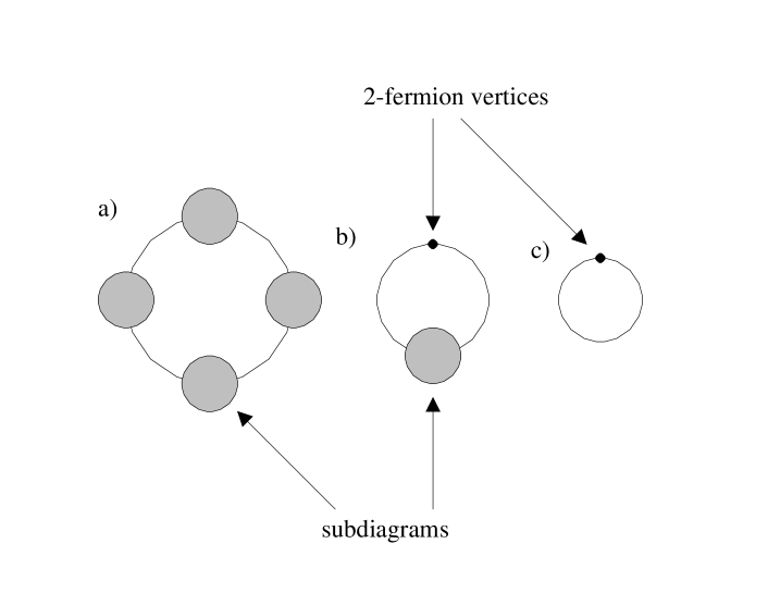
We first define a few useful concepts [9]. A cycle of lines or an m-cycle in a vacuum diagram is a set of fermion lines with the property that when we cut all these lines the vacuum diagram separates into disjoint 2-point diagrams (see Figure 1a). When one and only one of these 2-point diagrams consists of only one 2-fermion vertex the cycle of lines is called trivial with respect to this type of 2-fermion vertex (see Figure 1b and c).
Next we define the (connected, collective coordinate integrated) 2-particle irreducible (2PI) vacuum diagrams as those vacuum diagrams that contain only nontrivial 1-cycles and trivial 2-cycles with respect to the 2-fermion vertex . (Note that the only trivial 1-cycle, Tr, shown in Figure 1c, is thus excluded.) The sum of all 2PI vacuum diagrams is denoted by .
One can now readily define the (connected, collective coordinate integrated) 2PI 2-point diagrams in terms of the 2PI vacuum diagrams through a functional derivation in the 2-fermion vertex . The sum of all amputated 2PI 2-point diagrams is given by
| (49) |
In this expression we show the dependence on the propagator to indicate that the lines in these diagrams represent the modal propagator, . We note that has the same collective coordinate integrals that has, because is independent of the collective coordinates.
One can construct the sum of all 2-point diagrams from the sum of all 2PI 2-point diagrams, , by simply replacing the modal propagator with the full propagator . Thus represents the sum of all 2-point diagrams.***The diagrams in are by definition 2PI with respect to the full propagator . However when the full propagator inside these diagrams are replaced by the sum of diagrams in which fermion lines represent , the diagrams in are not necessarily 2PI anymore.
Now we introduce the topological equation [9]:
| (50) |
where is the number of cycles of lines in a vacuum diagram, is the total number of lines in the diagram, and is the number of 2PI skeletons. A 2PI skeleton is what remains of a 2PI vacuum diagram after one has cut out all 2-fermion vertices. The topological equation (50) holds for every vacuum diagram separately.
One can use this topological equation to construct a resummation equation for the sum of all vacuum diagrams. This resummation equation, which will make it possible to write the sum of all vacuum diagrams in terms of the 2-point functions, is given by
| (51) |
Each term on the right-hand side of this equation is formed by counting each vacuum diagram as many times as the number of the corresponding elements (cycles, lines or skeletons) that appear in it. According to (51) these three terms give back the sum of all vacuum diagrams, .
One forms by constructing all cycles:
| (52) |
The minus sign inside the summation is because of the fermion loop. To form one closes off the sum of all 2-point diagrams (minus the modal propagator) with :
| (53) |
The minus sign in front is because we are closing off a fermion loop. The term is formed by replacing all the ’s inside the sum of all 2PI vacuum diagrams, , by the full propagator and add to this Tr, because is also a 2PI skeleton and Tr is excluded from the definition of 2PI vacuum diagrams. So we have
| (54) |
When we place (52), (53) and (54) into (51) the result is
| (55) |
One can simplify this by using the following expression that relates and ,
| (56) |
which represents the resummation of self-energy diagrams. Then we have
| (57) |
The Legendre transform for 2-point functions removes the last term, leaving us with an effective action for 2-point functions
| (58) |
The 2PI vacuum diagrams in are constructed with Feynman rules that differ from those mentioned in Section V only in that there is no 2-fermion nonlocal source vertex anymore and the modal propagator is now replaced by the full propagator . The other terms in (58) are referred to as the ‘one-loop’ terms.
This expression resembles the CJT effective action [10],
| (59) |
The differences are that contains the modal propagator , instead of the bare propagator ; the traces, Tr, in include an integration over the collective coordinates, and includes the term , which, after the collective coordinate integration, becomes a constant that is removed through normalization.
Taking the functional derivative of with respect to the full propagator, one obtains a gap equation for the full propagator:
| (60) |
The collective coordinate integral of in momentum space equals the bare propagator multiplied by a momentum-dependent scalar form factor. If one restricts to be the one–instanton (and one–anti-instanton) amplitude and considers the small mass limit, one can show that the gap equation in (60) reproduces the Carlitz and Creamer gap equation [6] to leading order in small mass.
B The 4-point effective action
The generation of 4-point functions by instantons is elucidated by the complete effective action which is found by performing a second Legendre transform:
| (61) |
This operation actually only affects the sum of all 2PI vacuum diagrams, , in (58). The remaining terms in that expression are independent of .
Here, as explained in Section I, we are interested in the case when the fermions remain massless. By fixing the full fermion propagator to one that has no mass term, one can distinguish right-handed and left-handed fermion fields. The nonlocal 4-fermion source term in (4) is for this purpose replaced by
| (63) | |||||
These five chirality structures are the only ones that can be included without completely breaking the chiral symmetry and thereby generating a dynamical mass for the fermions. In this expression color, flavor and Dirac indices are implicitly contracted on the sources. It turns out to be more convenient to work with the five amputated 4-point functions that have the same chiral structures as the sources in (63). The chirality changing 4-point functions, and and the chirality conserving 4-point functions, , and are used instead of the corresponding ’s. The resulting 4-point effective action, , is stationary with respect to variations in the ’s. These stationarity conditions coincides with those of in , because is kept fixed.
In [2] the procedures of [9] are adapted to gauge theories and a 4-point effective action is obtained in terms of the five amputated ’s:
| (67) | |||||
The derivation of (67) is based on diagrammatic arguments from [2, 9] which are also applicable to the instanton case at hand. The only difference in this case is the set of Feynman rules, which are discussed below. We do not reproduce the derivation of (67) here. The one-loop terms of (58) are dropped from the 4-point effective action because they do not contain ’s and would therefore not affect the 4-point gap equations.
The first term in (67) contains the result of the summation of 4-particle reducible diagrams, i.e. those that can be separated into two disjoint parts by cutting two pairs of fermion lines. The two fermion lines in these pairs can flow in the same direction (-type) or in opposite directions (-type). The products of ’s and other operators in (67) indicate that the associated 4-point functions are connected to each other by a pair of fermion lines of either the -type or -type. The type of fermion pair involved is indicated by the subscript on the brackets. The other operators in (67) are defined as follows in terms of sequences of ’s:
| (68) | |||
| (69) |
The last term in (67), , is the sum of all 4PI†††The definition of 4PI is such that the possibility to remove only a by cutting four lines in a diagram does not imply that the diagram is not 4PI. However, the diagram consisting of two interconnected is not 4PI. See [2, 9] for the exact definition of 4PI. vacuum diagrams, calculated with the relevant Feynman rules. These Feynman rules differ from those mentioned in Section V in that there are no nonlocal source vertices anymore. Instead the 4-point functions now act as 4-fermion vertices. Furthermore, the modal propagator is replaced by the full propagator. We still have the -point instantons vertices, and and each diagram must still be integrated over the collective coordinates of all instantons in the diagram.
The term contains an infinite set of diagrams. Therefore any specific calculation would require a consistent truncation scheme, similar to those employed in applications of the Dyson-Schwinger equation.
VII Conclusions
The instanton effective action formalism presented here makes it possible to investigate the nonperturbative formation of 2-point and 4-point functions. In this way one can determine whether and under what circumstances these n-point functions can act as order parameters that signal the (partial) breaking of a chiral symmetry. Our effective actions are derived using the diagrammatic procedures developed in [2, 9]. These diagrammatic procedures require as input a diagrammatic language, Feynman rules, in terms of which the diagrams can be expressed. We have presented here such a diagrammatic language for instantons. The key features of it are:
-
the nonlocal -point instanton vertices, which can be seen as the natural generalization of the effective ’t Hooft vertex to high energy scales;
-
the modal propagator that propagates the different fermion modes, including the zeromodes, while avoiding the singularities of the Dirac operator.
One success of this formalism that is already apparent without doing any specific calculations is the fact that the 2-point effective action reproduces the Carlitz and Creamer gap equation [6] in the small mass limit.
It is perhaps useful to compare this formalism to the instanton liquid model [7, 8]. The most obvious difference is the fact that the instanton liquid formalism is a statistical physics approach whereas the formalism here is a quantum field theory approach. The instanton liquid model contains statistical quantities like average instanton size and average instanton separation. The effective action formalism, on the other hand, is formulated in terms of the resummation of Feynman diagrams containing the instanton dynamics in terms of vertices and propagators.
Another obvious difference is the fact that the instanton liquid approach specifically includes the instanton interactions, , which we dropped. Due to this it might appear that our formalism neglects an important part of the physics that governs the behavior of instantons. The point is that the instanton liquid model addresses a different regime than what we intend to address through our formalism. Instanton liquid models are mostly employed in the low energy phenomenology of QCD. In this regime the coupling constant is fairly large and the instanton ensemble, although dilute enough to use a semi-classical approximation, is not dilute enough to neglect instanton interactions. For example, Dyakonov and Petrov pointed out in [14] that the coefficient of the instanton interaction term is large in the absence of fermions. One of the crucial aspects in their analysis is the stabilization of the instanton ensemble. The instanton interactions, which are on average repulsive, provide the mechanism for this stabilization.
In contrast to this, the effective action formalism attempts to answer questions about the generation of order parameters. These are expected to appear at high energy scales when the coupling constant is still fairly small. Furthermore, if the phase transitions associated with these symmetry breakings are continuous – second order or higher – the order parameters would be small close to the transition point. The order parameters are therefore ideal expansion parameters. Terms containing small powers of the order parameters will dominate the analysis. The diluteness factor is related to the tunneling amplitude, which contains positive powers of the order parameter. One can thus see that terms with factors of diluteness come with high powers of the order parameter and are therefore suppressed in the region where these order parameters are small.
Yet it must be acknowledged that the diluteness terms do represent important physics. This can be seen from the fact that without them the effective potential would not be bounded below.‡‡‡It is a well known fact[16] that the 2-point effective potential – which in our case does not differ significantly from the CJT effective potential – is unbounded below even without dynamics. This is a problem related to the nonlocality of the 2-fermion sources. The dynamics given by the instanton vertices is purely attractive and by increasing the size of the order parameter one lowers the energy of the potential. The repulsiveness of the diluteness terms are required to make the potential bounded from below. This aspect is however irrelevant for the investigation into the nature of the second order phase transitions that interests us.
It is in principle possible to include the diluteness terms in the effective action formalism. One simply needs to derive “Feynman rules” for these types of interactions. However, the resulting formalism would be awkward. One of the reasons for neglecting them is because they depend on statistical physics quantities. Their inclusion would therefore lead to a mixed statistical physics–quantum field theory formalism.
Acknowledgements
We are grateful to Bob Holdom for helpful discussions. One of us (FSR) also wants to thank Stephen Selipsky for explaining certain aspects of instantons to him.
REFERENCES
- [1] B. Holdom, Phys. Rev. D54, 1068 (1996); Phys. Rev. D57, 357 (1998).
- [2] F. S. Roux, T. Torma and B. Holdom, to appear in Phys. Rev. D, (1999).
- [3] A. A. Belavin, A. M. Polyakov, A. S. Schwartz and Y. S. Tyupkin, Phys. Lett. B59, 85 (1975).
- [4] G. ’t Hooft, Phys. Rev. D14, 3432 (1976).
-
[5]
D. G. Caldi, Phys. Rev. Lett. 39, 121 (1977);
C. G. Callan, R. F. Dashen and D. J. Gross, Phys. Rev. D17, 2717 (1977). - [6] R. D. Carlitz and D. B. Creamer, Ann. of Phys. 118, 429 (1979).
- [7] D. I. Diakonov,“Chiral-symmetry breaking by instantons,” hep-ph/9602375.
- [8] E. V. Shuryak, Rev. Mod. Phys. 70, 323 (1998).
- [9] C. de Dominicis and P. C. Martin, J. Math. Phys. 5, 31 (1964).
- [10] J. M. Cornwell, R. Jackiw and E. Tomboulis, Phys. Rev. D10 2428 (1974).
- [11] L. S. Brown and D. B. Creamer, Phys. Rev., D18, 3695 (1978).
- [12] C. Lee and W. A. Bardeen, Nucl. Phys. B153, 210 (1979).
- [13] L. S. Brown, R. D. Carlitz, D. B. Creamer and C. Lee, Phys. Lett. B71, 103 (1977).
- [14] D. I. Diakonov and V. Y. Petrov, Nucl. Phys. B205, 259 (1984).
- [15] M. Lüscher, Nucl. Phys. B245, 483 (1982).
- [16] T. Banks and S. Raby, Phys. Rev. D14, 2182 (1976).