Width difference in the $B_{s}$-$\bar{B}_{s}$ system with lattice NRQCD

Abstract

We present a lattice calculation of the $B_{s}-\bar{B}_{s}$ transition matrix element through a four-quark operator ${\cal O}_{S}$ = $\bar{b}(1-\gamma_{5})s\ \bar{b}(1-\gamma_{5})s$, which gives a leading contribution in the calculation of the width difference $\Delta\Gamma_{s}$ in the $1/m_{b}$ expansion. The NRQCD formulation is used to describe $b$ quark on the lattice. Using the next-to-leading formula of Beneke et al., we obtain $(\Delta\Gamma/\Gamma)_{s}$ = 0.151(37)(45)(17), where the first error reflects the uncertainty of the $B_{s}$ meson decay constant, the second error comes from our calculation of the matrix element of ${\cal O}_{S}$, and the third represents unknown $1/m_{b}$ correction.

I Introduction

The mixing and decays of the $B_{s}^{0}-\bar{B}_{s}^{0}$ system play a complementary role to the $B^{\pm}$ and $B_{d}^{0}-\bar{B}_{d}^{0}$ systems in studying the flavor mixing and CP violation [1]. In particular, if the width difference of the $B_{s}^{0}-\bar{B}_{s}^{0}$ system is sufficiently large, the angle $\phi_{3}$($\gamma$) of the unitarity triangle can be measured through untagged modes such as $B_{s}\rightarrow D_{s}^{(*)}K^{(*)}$ or $B_{s}\rightarrow D^{*}\phi$ [2, 3], which would be promising not only because the method is theoretically clean but also feasible at future hadron colliders.

The width difference $\Delta\Gamma_{B_{s}}$ of the $B_{s}-\bar{B}_{s}$ systems is calculated most reliably using the heavy quark expansion [4], and the size of a ratio $(\Delta\Gamma/\Gamma)_{B_{s}}$ is roughly estimated as $(\Delta\Gamma/\Gamma)_{B_{s}}$ = 0.16(${}^{+0.11}_{-0.09}$). Now that the perturbative error has been reduced by the recent calculation of the next-to-leading order (NLO) QCD corrections [5], the largest remaining uncertainty comes from the matrix elements $\langle\bar{B}_{s}|{\cal O}_{X}(\mu_{b})|B_{s}\rangle$ ($X=L$ or $S$) of four-quark operators

$${\cal O}_{L} = \bar{b}\gamma_{\mu}(1-\gamma_{5})s\ \bar{b}\gamma_{\mu}(1-\gamma_{5})s,$$ (1)

$${\cal O}_{S} = \bar{b}(1-\gamma_{5})s\ \bar{b}(1-\gamma_{5})s.$$ (2)

Lattice QCD is one of the most suitable tools for the nonperturbative computation of matrix elements such as the decay constants and the bag parameters. In fact a number of extensive studies, including ours [6], have already been done to obtain $B_{L}$ [7], which is a matrix element of the former operator ${\cal O}_{L}$ normalized by its vacuum saturation approximation. On the other hand, the matrix element $B_{S}$ for the latter operator ${\cal O}_{S}$ has been calculated in Ref. [8] only for the heavy-light meson around charm quark mass regime. It is required to perform a thorough study of $B_{S}$ in order to give a reliable prediction of the $B_{s}$ width difference. The matrix element of ${\cal O}_{S}$ is also required in the evaluation of the amplitude $\Delta M$ of the $B_{(s)}-\bar{B}_{(s)}$ mixing, if we assume the physics beyond the Standard Model such as the supersymmetric models [9].

In this paper, we present a quenched lattice calculation of the matrix element of ${\cal O}_{S}$ using the NRQCD formalism [10] for heavy quark and the $O(a)$-improved Wilson action [11] for light quark. The NRQCD formalism is formulated as an inverse heavy quark mass expansion, and our action and operators consistently include entire $O(p/m_{Q})$ terms, where $p$ denotes a typical spatial momentum of a heavy quark inside a heavy-light meson. Higher order contribution of $O(p^{2}/m_{Q}^{2})$ is also studied by introducing all necessary terms, and we find those effect is small for the $b$ quark mass.

In this work one-loop matching of the operator ${\cal O}_{S}$ between continuum and lattice regularizations is performed in the limit of infinitely heavy quark mass, so that the systematic error of $O(\alpha_{s}/(am_{Q}))$ is not removed. Since the $b$ quark mass in the lattice unit is not extremely large, $O(\alpha_{s}/(am_{Q}))$ gives a non-negligible effect in our final result, which could be as large as about 10% in a naive order counting argument.

Using the NLO formula of Ref. [5] and our results for the matrix elements of ${\cal O}_{S}$ as well as of ${\cal O}_{L}$ [6], we obtain a prediction $(\Delta\Gamma/\Gamma)_{B_{s}}$ = 0.151(37)(45)(17). The first error originates in the $B_{s}$ meson decay constant $f_{B_{s}}$ = 245(30) MeV [7] used to normalize the matrix elements, and the second is from our calculation of the matrix element of ${\cal O}_{S}$. The error from $B_{L}$ is negligible, since it gives only a small contribution to the width difference. The last error is a crude estimate of the $O(1/m_{b})$ correction as discussed in Refs. [4, 5].

This paper is organized as follows. We briefly summarize the NLO formula of Ref. [5] for the width difference in the next section. We present the perturbative matching of the operator ${\cal O}_{S}$ in Section III, while the detail of the one-loop calculation is given in Appendix. We describe our simulation methods in Section IV, and our results for the matrix element and the width difference are given in Section V. In section VI, we attempt to estimate the size of $O(\alpha_{s}/(am_{Q}))$ error, which is specific to our work with NRQCD. Section VII is devoted to a comparison of our result with a previous work by Gupta et al. [8], who obtained the same matrix element using the relativistic lattice action around charm quark mass. Finally our conclusion is given in Section VIII. A preliminary report of this work is included in Ref. [12].

II Width difference of $B_{s}$ mesons

In this section we briefly summarize the formula to give the width difference of $B_{s}$ mesons, which was obtained by Beneke et al. in Ref. [5].

The width difference in the $B_{s}-\bar{B}_{s}$ system is given by

$$\Delta\Gamma_{B_{s}}=-2\frac{1}{2M_{B_{s}}}\langle\bar{B}_{s}|\mbox{Im\ }i\int d^{4}xT{\cal H}_{eff}(x){\cal H}_{eff}(0)|B_{s}\rangle,$$ (3)

where ${\cal H}_{eff}$ is a $\Delta B$=1 weak transition Hamiltonian. The main contribution comes from a transition $b\bar{s}\rightarrow c\bar{c}$ followed by $c\bar{c}\rightarrow\bar{b}s$, and other contributions mediated by penguin operators are also included [5].

Using the $1/m_{b}$ expansion, the transition operator $\mbox{Im\ }i\int d^{4}xT{\cal H}_{eff}(x){\cal H}_{eff}(0)$ is represented by the local four-quark operators ${\cal O}_{L}$ and ${\cal O}_{S}$, which leads to the following formula at the next-to-leading order [5],

$$\left(\frac{\Delta\Gamma}{\Gamma}\right)_{B_{s}} = \frac{16\pi^{2}B(B_{s}\rightarrow Xe\nu)}{g(z)\tilde{\eta}_{QCD}}\frac{f_{B_{s}}^{2}M_{B_{s}}}{m_{b}^{3}}|V_{cs}|^{2}$$ (5)

$$\times\left(G(z)\frac{8}{3}B_{L}(m_{b})+G_{S}(z)\frac{5}{3}\frac{B_{S}(m_{b})}{{\cal R}(m_{b})^{2}}+\sqrt{1-4z}\delta_{1/m}\right).$$

Here, the quantity $B(B_{s}\rightarrow Xe\nu)$ is the semi-leptonic decay branching ratio. The factors $g(z)=1-8z+8z^{3}-z^{4}-12z^{2}\ln z$ ($z=m_{c}^{2}/m_{b}^{2}$) and $\tilde{\eta}_{QCD}$ represent the phase space factor and the QCD correction, respectively. The coefficients $G(z)$ and $G_{S}(z)$ are functions including the next-to-leading QCD corrections, and their numerical values are given in Table 1 of Ref. [5].

$B_{L}(m_{b})$ and $B_{S}(m_{b})$ are the $B$ parameters defined with the $\overline{MS}$ scheme at the renormalization scale $\mu_{b}=m_{b}$. Their definitions are

$$B_{L}(\mu_{b}) \equiv \frac{\langle\bar{B}_{s}|{\cal O}_{L}(\mu_{b})|B_{s}\rangle}{\frac{8}{3}\langle\bar{B}_{s}|A_{0}|0\rangle\langle 0|A_{0}|B_{s}\rangle}=\frac{\langle\bar{B}_{s}|{\cal O}_{L}(\mu_{b})|B_{s}\rangle}{\frac{8}{3}f_{B_{s}}^{2}M_{B_{s}}^{2}},$$ (6)

$$B_{S}(\mu_{b}) \equiv \frac{\langle\bar{B}_{s}|{\cal O}_{S}(\mu_{b})|B_{s}\rangle}{\frac{5}{3}\langle\bar{B}_{s}|P(\mu_{b})|0\rangle\langle 0|P(\mu_{b})|B_{s}\rangle}=\frac{\langle\bar{B}_{s}|{\cal O}_{S}(\mu_{b})|B_{s}\rangle}{-\frac{5}{3}f_{B_{s}}^{2}M_{B_{s}}^{2}}\times{\cal R}(\mu_{b})^{2}.$$ (7)

In the last expression in Eq. (7), we change the normalization of $\langle\bar{B}_{s}|{\cal O}_{S}(\mu_{b})|B_{s}\rangle$ with the decay constant $f_{B_{s}}$ by factoring out the ratio

$${\cal R}(\mu_{b})\equiv\left|\frac{\langle 0|A_{0}|B_{s}\rangle}{\langle 0|P(\mu_{b})|B_{s}\rangle}\right|.$$ (8)

Using the equation of motion the ratio ${\cal R}(\mu_{b})$ is expressed in terms of the quark masses $m_{b}$ and $m_{s}$ as

$${\cal R}(\mu_{b})=\frac{\bar{m}_{b}(\mu_{b})+\bar{m}_{s}(\mu_{b})}{M_{B_{s}}},$$ (9)

where $\bar{m}_{b}(\mu_{b})$ and $\bar{m}_{s}(\mu_{b})$ denote the quark masses defined with the $\overline{MS}$ scheme at scale $\mu_{b}$.

Finally $\delta_{1/m}$ denotes $1/m_{b}$ corrections, which may be estimated using the factorization approximation [4].

Numerically evaluating the coefficients in the right hand side of Eq. (5), we obtain

$$\left(\frac{\Delta\Gamma}{\Gamma}\right)_{B_{s}}=\left(\frac{f_{B_{s}}}{245{\rm MeV}}\right)^{2}\left[0.008B_{L}(m_{b})+0.150\frac{B_{S}(m_{b})}{{\cal R}(m_{b})^{2}}-0.086\right],$$ (10)

where we choose a recent world average of unquenched lattice simulations $f_{B_{s}}$ = 245(30) MeV for the central value of the decay constant [7]. In the following sections we present a calculation of the parameter $B_{S}(m_{b})/{\cal R}(m_{b})^{2}$. Our calculation of $B_{L}(m_{b})$ is already available in Ref. [6].

III Operator matching

In this section, we present the perturbative matching of continuum operator ${\cal O}_{S}$ to the corresponding operators defined on the lattice. We follow the calculation method in Ref. [13], where the one-loop matching of the operator ${\cal O}_{L}$ is presented.

Following the definition in Ref. [5], we adopt modified minimal subtraction ($\overline{MS}$) with the Naive Dimensional Regularization (NDR) scheme for the continuum operator ${\cal O}_{S}(\mu_{b})$, in which $\gamma_{5}$ anticommutes with all $\gamma_{\mu}$’s. The subtraction of evanescent operators is done with the definition given by Eqs. (13)-(15) of Ref. [5]. The renormalization scale $\mu_{b}$ is set to the $b$ quark mass $m_{b}$.

While in the numerical simulations we apply the NRQCD formalism [10] to the heavy quarks, in the perturbative calculation the heavy quarks are treated as a static quark [14]. More comments on this approximation will be given in the end of this section. The light quarks and gauge fields are described by the $O(a)$-improved SW quark action [11] and the standard Wilson (plaquette) action, respectively, in both of the perturbative calculation and the numerical simulations.

The operators involved in the calculation are

$${\cal O}_{S} = \bar{b}^{i}P_{L}s^{i}\ \bar{b}^{j}P_{L}s^{j},$$ (11)

$$\tilde{{\cal O}}_{S} = \bar{b}^{i}P_{L}s^{j}\ \bar{b}^{j}P_{L}s^{i},$$ (12)

$${\cal O}_{L} = \bar{b}^{i}\gamma_{\mu}P_{L}s^{i}\ \bar{b}^{j}\gamma_{\mu}P_{L}s^{j},$$ (13)

$${\cal O}_{P} = 2\ \bar{b}^{i}\gamma_{\mu}P_{L}s^{i}\ \bar{b}^{j}\gamma_{\mu}P_{R}s^{j}+4N\ \bar{b}^{i}P_{L}s^{i}\ \bar{b}^{j}P_{R}s^{j},$$ (14)

$${\cal O}_{R} = \bar{b}^{i}\gamma_{\mu}P_{R}s^{i}\ \bar{b}^{j}\gamma_{\mu}P_{R}s^{j},$$ (15)

$${\cal O}_{SD} = \bar{b}^{i}P_{L}(\vec{\gamma}\cdot a\vec{D})s^{i}\ \bar{b}^{j}P_{L}s^{j},$$ (16)

$${\cal O}_{LD} = \bar{b}^{i}\gamma_{\mu}P_{L}(\vec{\gamma}\cdot a\vec{D})s^{i}\ \bar{b}^{j}\gamma_{\mu}P_{L}s^{j},$$ (17)

$${\cal O}_{PD} = 2\ \bar{b}^{i}\gamma_{\mu}P_{R}(\vec{\gamma}\cdot a\vec{D})s^{i}\ \bar{b}^{j}\gamma_{\mu}P_{L}s^{j}+4N\ \bar{b}^{i}P_{R}(\vec{\gamma}\cdot a\vec{D})s^{i}\ \bar{b}^{j}P_{L}s^{j},$$ (18)

where $P_{L}$ and $P_{R}$ are chirality projection operators $P_{L/R}=1\mp\gamma_{5}$. Color indices $i$ and $j$ run from one to $N$ for SU($N$) gauge theory and $a$ denotes lattice spacing. In the continuum, in which the chiral symmetry for light quark is preserved, the operator ${\cal O}_{S}$ mixes only with $\tilde{{\cal O}}_{S}$ and ${\cal O}_{L}$. On the lattice, however, the chiral symmetry is explicitly broken with the SW action, so that additional operators with opposite chirality, ${\cal O}_{P}$ and ${\cal O}_{R}$, appear in the operator matching.

Other operators ${\cal O}_{SD}$, ${\cal O}_{LD}$ and ${\cal O}_{PD}$ are higher dimensional operators introduced to cancel a discretization error of $O(\alpha_{s}a)$. However we neglect this discretization error in the numerical simulations. The result of $O(a\alpha_{s})$ matching coefficients is presented only for future use.

Here we show the one-loop result of the matching. We leave the detail of the calculations for Appendix A. The continuum operator ${\cal O}_{S}(\mu_{b})$ is expressed by lattice operators ${\cal O}_{X}^{\rm lat}(1/a)$ as follows [15],

$${\cal O}_{S}(\mu_{b}) = \Bigg{[}\ 1+\frac{\alpha_{s}}{4\pi}\Bigg{\{}\frac{4}{3}\ln\left(a^{2}m_{b}^{2}\right)+\frac{16}{3}\ln\left(\frac{\mu_{b}^{2}}{m_{b}^{2}}\right)-3.86\Bigg{\}}\Bigg{]}{\cal O}_{S}^{\rm lat}(1/a)$$ (22)

$$+\frac{\alpha_{s}}{4\pi}\Bigg{[}\ -\frac{2}{3}\ln\left(a^{2}m_{b}^{2}\right)+\frac{1}{3}\ln\left(\frac{\mu_{b}^{2}}{m_{b}^{2}}\right)+3.91\Bigg{]}{\cal O}_{L}^{\rm lat}(1/a)$$

$$+\frac{\alpha_{s}}{4\pi}\ \Big{[}\ 0.77\ \Big{]}{\cal O}_{P}^{\rm lat}(1/a)+\frac{\alpha_{s}}{4\pi}\ \Big{[}\ 0.13\ \Big{]}{\cal O}_{R}^{\rm lat}(1/a)$$

$$+\frac{\alpha_{s}}{4\pi}\ \Big{[}\ -6.88\ \Big{]}{\cal O}_{SD}^{\rm lat}(1/a)+\frac{\alpha_{s}}{4\pi}\ \Big{[}\ 2.58\ \Big{]}{\cal O}_{LD}^{\rm lat}(1/a)+\frac{\alpha_{s}}{4\pi}\ \Big{[}\ 1.15\ \Big{]}{\cal O}_{PD}^{\rm lat}(1/a).$$

The operator $\tilde{{\cal O}}_{S}$ is eliminated from the right hand side using a identity $\tilde{{\cal O}}_{S}=-{\cal O}_{S}-\frac{1}{2}{\cal O}_{L}$, which is valid up to $O(p/m_{Q})$.

The heavy-light axial vector current $A_{0}$ is also necessary to normalize the matrix element. The one-loop matching of $A_{0}$ is already known as [16, 17, 13]

$$A_{0} = Z_{A}(1/a)A_{0}^{\rm lat}(1/a)+Z_{A_{D}}(1/a)A_{D0}^{\rm lat}(1/a)$$ (23)

$$= \Bigg{[}1+\frac{\alpha_{s}}{4\pi}\left[\ 2\ln(a^{2}m_{b}^{2})-16.561\ \right]\ \Bigg{]}\ A_{0}^{\rm lat}(1/a)-\frac{\alpha_{s}}{4\pi}[\ 13.01\ ]\ A_{D0}^{\rm lat}(1/a),$$ (24)

where $A_{0}$ and $A_{D0}$ are defined as

$$A_{0} = \bar{b}\gamma_{0}\gamma_{5}s,$$ (25)

$$A_{D0} = \bar{b}\gamma_{0}\gamma_{5}(\vec{\gamma}\cdot a\vec{D})s.$$ (26)

The higher dimensional operator $A_{D0}$ is introduced to remove the $O(\alpha_{s}a)$ errors.

In Eqs. (22) and (24), we apply the tadpole improvement [18] using $u_{0}=1/8\kappa_{c}$ as an average link variable. The normalization of the light quark filed is $\sqrt{1-3\kappa/4\kappa_{c}}$.

To obtain the matching coefficient for $B_{S}/{\cal R}^{2}$ we combine Eqs. (22) and (24), and linearize the perturbative expansion in $\alpha_{s}$. Omitting the higher dimensional operators, which we neglect in the following numerical simulations, we obtain

$$B_{S}(\mu_{b})/{\cal R}(\mu_{b})^{2} = \Bigg{[}\ 1+\frac{\alpha_{s}}{4\pi}\Bigg{\{}-\frac{8}{3}\ln\left(a^{2}m_{b}^{2}\right)+\frac{16}{3}\ln\left(\frac{\mu_{b}^{2}}{m_{b}^{2}}\right)+29.26\Bigg{\}}\Bigg{]}\hat{B}_{S}^{\rm lat}$$ (29)

$$+\frac{\alpha_{s}}{4\pi}\Bigg{[}\ -\frac{2}{3}\ln\left(a^{2}m_{b}^{2}\right)+\frac{1}{3}\ln\left(\frac{\mu_{b}^{2}}{m_{b}^{2}}\right)+3.91\Bigg{]}\hat{B}_{L}^{\rm lat}$$

$$+\frac{\alpha_{s}}{4\pi}\ \Big{[}\ 0.77\ \Big{]}\hat{B}_{P}^{\rm lat}+\frac{\alpha_{s}}{4\pi}\ \Big{[}\ 0.13\ \Big{]}\hat{B}_{R}^{\rm lat},$$

where $\hat{B}_{X}^{\rm lat}$ ($X$ = $S$, $L$, $P$, or $R$) are ‘$B$ parameters’ defined by

$$\hat{B}_{X}^{\rm lat}=\frac{\langle{\cal O}_{X}^{\rm lat}(1/a)\rangle}{-\frac{5}{3}\langle A_{0}^{\rm lat}(1/a)\rangle^{2}},$$ (30)

which we measure in the numerical simulations.

Before closing this section, we should clarify the remaining uncertainty arising from the static approximation in the matching coefficients. In the simulation, the heavy quarks are described by the NRQCD action including the $O(p/m_{Q})$ or $O(p^{2}/m_{Q}^{2})$ corrections consistently. The $b$ quark field, which constitutes the operators measured in the simulation, is also improved through the same order as the action by the inverse Foldy-Wouthuysen-Tani transformation $R^{-1}$ as

$$b = R^{-1}\left(\begin{array}[]{c}Q\\ \chi^{\dagger}\end{array}\right),$$ (33)

where $Q$ and $\chi^{\dagger}$ are the two-component quark and anti-quark fields in the NRQCD action. Therefore the truncation error only starts from $O(p^{2}/m_{Q}^{2})$ or $O(p^{3}/m_{Q}^{3})$, which depends on the accuracy of our action and operators, even at the tree level matching. On the other hand, the static approximation in the perturbative calculation only leads to a lack of finite mass effects in the matching coefficients, but does not change the truncation error. Therefore, using the matching coefficients derived in this section the result has the $O(\alpha_{s}/(am_{Q}))$ error.

IV Simulations

The numerical simulations to extract $\hat{B}_{X}^{\rm lat}$ are almost the same as in our previous paper [6], in which we calculated $B_{L}$. We carried out a quenched simulation on 250 $16^{3}\times 48$ lattices at $\beta$=5.9. The inverse lattice spacing from the string tension is 1.64 GeV. We employ the SW action for light quark [11] with mean field improved $c_{sw}=1/{u_{0}}^{3}$ with $u_{0}=0.8734$. The heavy quark is treated by two sets of NRQCD actions and fields [10] as was done in Ref. [6]: one is truncated at $O(p/m_{Q})$ and the other includes entire $O(p^{2}/m_{Q}^{2})$ corrections. We use the difference between the results from these sets to estimate the size of truncation error of the $p/m_{Q}$ expansion.

For the strong coupling constant used in the perturbative matching, we choose the $V$-scheme coupling $\alpha_{V}(q^{*})$ with $q^{*}=1/a$, $2/a$ or $\pi/a$. Their numerical values are $\alpha_{V}(1/a)$ = 0.270, $\alpha_{V}(2/a)$=0.193 and $\alpha_{V}(\pi/a)$ = 0.164.

Other details of our simulations, such as the exact definition of the NRQCD action and the mass parameters used, are found in the previous paper [6].

V Results

Figure 1 shows the mass dependence of $\hat{B}^{\rm lat}_{X}$ ($X$ = $S$, $L$ or $P$) defined in Eq. (30). $\hat{B}^{\rm lat}_{R}$ is equal to $\hat{B}^{\rm lat}_{L}$ because of a symmetry under parity transformation. The light quark mass is interpolated to the strange quark mass. Since the light quark mass dependence is very small, in the following analysis we do not consider the error arising from the interpolation. The inverse heavy-light meson mass $1/M_{P_{s}}$, for which the light quark mass is also interpolated to the strange quark mass, is used as a horizontal axis.

The difference between two results with different accuracies of the $p/m_{Q}$ expansion does not exceed a few percent at the $b$ quark mass, as explicitly presented in the figure by different symbols: circles for $O(p/m_{Q})$ and triangles for $O(p^{2}/m_{Q}^{2})$ accuracy. It justifies the use of the nonrelativistic expansion for the $b$ quark.

As we pointed out in the previous paper [6], the vacuum saturation approximation (VSA) gives a good approximation of the lattice data. In the static limit, it becomes $\hat{B}_{S}^{(VSA)}$=1, $\hat{B}_{L}^{(VSA)}$ = $-8/5$ and $\hat{B}_{P}^{(VSA)}$ = $-64/5$. For the finite heavy quark mass, the axial current and the pseudoscalar density involved in the VSA have different matrix elements. As a result, a mass dependence appears in the VSA of $\hat{B}_{X}$, as plotted by crosses (a flat line for $\hat{B}_{L}$) in Fig. 1. It is remarkable that the VSA explains the $1/M_{P_{s}}$ dependence of the data very nicely.

We combine the results for $\hat{B}^{\rm lat}_{X}$ to obtain $B_{S}(\mu_{b})/{\cal R}(\mu_{b})^{2}$ using Eq. (29). The renormalization scale $\mu_{b}$ is set to the $b$ quark pole mass $m_{b}$ = 4.8 GeV according to Ref. [5]. Figure 2 presents the $1/M_{P_{s}}$ dependence of $B_{S}(m_{b})/{\cal R}(m_{b})^{2}$ obtained with the $O(p/m_{Q})$ (circles) and $O(p^{2}/m_{Q}^{2})$ (triangles) accuracies and using $\alpha_{V}(2/a)$=0.193 as a coupling constant in the perturbative matching. Typical size of the perturbative error may be evaluated by comparing the results obtained with different coupling constants. For this purpose, we also calculate the results with $\alpha_{V}(\pi/a)$=0.164 and $\alpha_{V}(1/a)$=0.270, which are considered in the larger error bars in Fig. 2. We find that they give at most 5% differences at the $b$ quark mass.

Our numerical results interpolated to the physical $B_{s}$ meson mass $M_{B_{s}}$ = 5.37 GeV are

• for $O(p/m_{Q})$ accuracy

  $$\frac{B_{S}(m_{b})}{{\cal R}(m_{b})^{2}}=\left\{\begin{array}[]{lll}1.51(3)&\mbox{\ at\ }&q^{*}=\pi/a\\ 1.54(3)&\mbox{\ at\ }&q^{*}=2/a\\ 1.61(3)&\mbox{\ at\ }&q^{*}=1/a\end{array}\right.,$$ (34)

• for $O(p^{2}/m_{Q}^{2})$ accuracy

  $$\frac{B_{S}(m_{b})}{{\cal R}(m_{b})^{2}}=\left\{\begin{array}[]{lll}1.56(3)&\mbox{\ at\ }&q^{*}=\pi/a\\ 1.59(3)&\mbox{\ at\ }&q^{*}=2/a\\ 1.67(3)&\mbox{\ at\ }&q^{*}=1/a\end{array}\right.,$$ (35)

where the error represents the statistical error. The variation due to the choice of the coupling constant $\alpha_{V}(q^{*})$ is explicitly shown.

We attempt to estimate the size of systematic uncertainty in our result using an order counting of missing contributions. As we found in the previous paper [6], the dominant uncertainties are

$$O(\alpha_{s}/(am_{Q}))\sim 15\%,$$ (36)

$$O(\alpha_{s}^{2})\sim 10\%,$$ (37)

$$O(a^{2}\Lambda_{QCD}^{2})\sim O(a\Lambda_{QCD}\alpha_{s})\sim 5\%,$$ (38)

when we assume $\Lambda_{QCD}\sim$ 300 MeV and $\alpha_{s}\sim$ 0.3. Although a naive order counting yields $O(\alpha_{s}/(am_{Q}))\sim$ 10%, we take more conservative estimate $\sim$ 15%, which is suggested in the study of bilinear operators as we will discuss in the next section. The effect of the truncation of the nonrelativistic expansion is negligible as we explicitly see in the difference between the two simulations of the $O(p/m_{Q})$ and $O(p^{2}/m_{Q}^{2})$ accuracies.

We finally obtain

$$\frac{B_{S}(m_{b})}{{\cal R}(m_{b})^{2}}=1.54(3)(30),$$ (39)

where the first error represents the statistical error, while the second is obtained by adding the sources of systematic uncertainty in quadrature.

Using this result and the result for $B_{L}(m_{b})$ previously obtained in Ref. [6], $B_{L}(m_{b})$ = 0.75(2)(12), we find

$$\left(\frac{\Delta\Gamma}{\Gamma}\right)_{B_{s}}=0.151(37)(45)(17),$$ (40)

from Eq. (10). The first error comes from the uncertainty in the decay constant $f_{B_{s}}$ = 245(30) MeV, which is taken from the current world average of unquenched lattice calculations [7]. The second reflects the error in the calculation of $B_{S}/{\cal R}^{2}$ presented above, and the last is obtained by assuming that the size of error in the $1/m_{b}$ correction $\delta_{1/m}$ in Eq. (5) is $\pm$ 20%. The current experimental bound is $(\Delta\Gamma/\Gamma)_{B_{s}}<$ 0.42 [19].

The central value of our result in Eq. (40) is much larger than the estimate 0.054${}^{+0.016}_{-0.032}$ obtained by Beneke et al. [5]. The main reasons are

• The unquenched lattice result of $f_{B_{s}}$ is about 15–20% larger than the previously known quenched result.

• The central value of our result for $B_{S}/{\cal R}^{2}$ is larger than the previous value obtained from the relativistic lattice calculation [8], which is used in Ref. [5]. We will compare our result with theirs in section VII.

VI finite mass effects in the matching coefficients

In this section, we attempt to estimate the size of $O(\alpha_{s}/(am_{Q}))$ error arising from the lack of necessary one-loop correction, by taking the ratio ${\cal R}(m_{b})$ defined in Eq. (8) as an example. Although the $O(\alpha_{s}/(am_{Q}))$ errors in bilinear operators and in the bag parameters are independent, it would still be useful to explicitly see the size of the error in a quantity, for which the correct one-loop coefficient is known.

We compare the values of ${\cal R}(m_{b})^{2}$ obtained with the following methods.

1. The quantity ${\cal R}(m_{b})^{2}$ may be explicitly calculated in lattice simulation by measuring the matrix elements of axial-vector and pseudoscalar density. Results of the JLQCD collaboration obtained with the NRQCD action [20] are plotted in Fig. 3 as a function of $1/M_{P_{s}}$. One-loop matching to the continuum operator are calculated for two different lattice actions: static (filled circles) and NRQCD (open circles) [21].

2. The equation of motion may be used to obtain

   $${\cal R}(m_{b})^{2}=\left(\frac{\bar{m}_{b}(m_{b})+\bar{m}_{s}(m_{b})}{M_{B_{s}}}\right)^{2}.$$ (41)

   For the phenomenological values $\bar{m}_{b}(m_{b})$=4.1–4.4 GeV and $\bar{m}_{s}(2{\rm GeV})$=0.06–0.17 GeV [22], which corresponds to $\bar{m}_{s}(m_{b})$=0.05–0.14 GeV, we obtain ${\cal R}(m_{b})^{2}$=0.66(5), which is shown by a star in Fig. 3.

The data obtained with the correct NRQCD matching coefficients (open circles) show a nice agreement with the phenomenological estimate (star). This suggests that the error in the calculation of the matrix element with correct matching coefficient is under good control. On the other hand, the data with the static matching coefficients (filled circles) are significantly lower, indicating a large systematic errors of $O(\alpha_{s}/(am_{Q}))$. The difference of ${\cal R}(m_{b})^{2}$ between the two matching calculations is around 15% for the $B_{s}$ meson mass. We use this number for the estimation of the systematic error of $O(\alpha/(am_{Q}))$ for $B_{S}(m_{b})/{\cal R}(m_{b})^{2}$ in Sec. V.

VII Discussion

It is instructive to compare our result with the previous lattice calculation by Gupta, Bhattacharya and Sharpe [8], who used the Wilson fermion action for heavy quark with the mass around charm quark. Conversion of their result to the definition used in this paper is given in Ref. [5], which yields $B_{S}(2.33~{}{\rm GeV})$=0.81 and $\tilde{B}_{S}(2.33~{}{\rm GeV})$=0.87. A $B$-parameter for the operator $\tilde{{\cal O}}_{S}$ (12) is denoted as $\tilde{B}_{S}$. With the renormalization group evolution, it becomes $B_{S}(m_{b})$=0.75 and $\tilde{B}_{S}(m_{b})$=0.85 at $\mu_{b}=m_{b}$. The error was not quoted except for the statistical one, which is 0.01 for each quantity. In order to compare the results obtained with different heavy quark mass, it is necessary to remove a logarithmic dependence on the heavy quark mass. We, therefore, define $\Phi_{B_{S}}(m_{b})$ as

$$\Phi_{B_{S}}(m_{b})=\Bigg{[}\ 1-2\frac{\alpha_{s}(m_{b})}{4\pi}\ln\bigg{(}\frac{m_{Q}^{2}}{m_{b}^{2}}\bigg{)}\ \Bigg{]}\ B_{S}(m_{b})+\frac{2}{5}\frac{\alpha_{s}(m_{b})}{4\pi}\ln\bigg{(}\frac{m_{Q}^{2}}{m_{b}^{2}}\bigg{)}\ \tilde{B}_{S}(m_{b}),$$ (42)

where $m_{Q}$ denotes the heavy quark mass used in the simulation. In the calculation of Gupta et al. [8] it is about the charm quark mass $m_{Q}$ = $m_{c}$ = 1.4 GeV. Using the coupling constant $\alpha_{s}(m_{b})$= 0.22 corresponding to $\Lambda_{\overline{MS}}^{(4)}$=0.327 GeV and ${\cal R}(m_{b})^{2}$ obtained with the method 2 in the previous section, we obtain

$$\Phi_{B_{S}}^{\rm GBS}(m_{b})/{\cal R}(m_{b})^{2}=1.20,$$ (43)

which may be compared with our result of $B_{S}(m_{b})/{\cal R}(m_{b})^{2}$ in Eq. (39).

The central value of our result is significantly higher than Eq. (43), which is one of the reasons of our larger value of $\left(\frac{\Delta\Gamma}{\Gamma}\right)_{B_{s}}$ compared to that of Ref. [5]. We note, however, that the calculation with the unimproved relativistic action could suffer from large $O(am_{Q})$ error, which is not even estimated in Ref. [8]. In our NRQCD calculation, on the other hand, all possible systematic uncertainties are considered, but unfortunately the large systematic error of $O(alpha_{s}/am_{Q})$ is left to be removed. Thus, at this stage we conclude that that the present accuracy of both calculations is not enough for a detailed comparison.

VIII Conclusion

The width difference $\Delta\Gamma_{s}$ in the $B_{s}-\bar{B}_{s}$ mixing is expressed by the matrix elements of local four-quark operators in the $1/m_{b}$ expansion. The operator ${\cal O}_{S}$ gives a dominant contribution among them and the nonperturbative calculation of its matrix element is essential for a reliable calculation of the width difference [4, 5]. We calculated a parameter $B_{S}(m_{b})/{\cal R}(m_{b})^{2}$, which is the matrix element normalized with a square of the $B_{s}$ meson decay constant as defined in Eq. (7), using lattice NRQCD formalism for heavy quark.

From a quenched simulation at $\beta$=5.9 with the $O(a)$-improved light quark action, we obtain $B_{S}(m_{b})/{\cal R}(m_{b})^{2}$ = 1.54(3)(30), where statistical and systematic errors are given in that order. By explicitly performing two calculations with the different accuracies, we found that the $O(p^{2}/m_{Q}^{2})$ corrections in the NRQCD action and operators is only a few percent. One of the dominant sources of the systematic error is a lack of one-loop matching coefficients with finite mass corrections. We used the one-loop coefficients for the static action instead, which introduces a systematic error of order $\alpha_{s}/(am_{Q})\sim$ 15%.

The large remaining uncertainty in our final result for $(\Delta\Gamma/\Gamma)_{s}$, Eq. (40), comes partly from the error in our calculation of $B_{S}(m_{b})/{\cal R}(m_{b})^{2}$. Another important source is present in the $B_{s}$ meson decay constant $f_{B_{s}}$, as it appears as $f_{B_{s}}^{2}$ in the formula.

We also discussed a comparison of our result with the previous one. We found that the central value of our result is significantly larger. However, since both calculations suffer from large systematic uncertainties, it would be fair to say that the discrepancy between the two results is not significant at the present level.

A

A matrix element of the continuum operator ${\cal O}_{S}$ with free quark external states is expressed at one-loop order as

$$\langle{\cal O}_{S}(\mu)\rangle = \Bigg{[}\ 1+\frac{\alpha_{s}}{4\pi}\Bigg{\{}\frac{13N^{2}-18N+9}{4N}+\frac{-3N^{2}+2N+5}{2N}\ln\left(\frac{\lambda^{2}}{m_{b}^{2}}\right)$$ (A5)

$$\hskip 156.49014pt+\frac{3N^{2}-4N-1}{N}\ln\left(\frac{\mu^{2}}{m_{b}^{2}}\right)\Bigg{\}}\Bigg{]}\langle{\cal O}_{S}\rangle_{0}$$

$$+\frac{\alpha_{s}}{4\pi}\Bigg{[}-\frac{11N-9}{2N}-\frac{N+1}{N}\ln\left(\frac{\lambda^{2}}{m_{b}^{2}}\right)-\frac{2(N-2)}{N}\ln\left(\frac{\mu^{2}}{m_{b}^{2}}\right)\Bigg{]}\langle\tilde{{\cal O}}_{S}\rangle_{0}$$

$$-\frac{\alpha_{s}}{4\pi}\frac{3(N-1)}{4N}\langle{\cal O}_{L}\rangle_{0}$$

$$+\frac{\alpha_{s}}{4\pi}\left[-\frac{2\pi}{3}\frac{1}{a\lambda}\right]\langle{\cal O}_{PD}\rangle_{0},$$

where $\langle{\cal O}_{X}\rangle_{0}$ denotes a tree level matrix element of operator ${\cal O}_{X}$, and the gluon mass $\lambda$ is introduced to regularize the infrared divergence. The evanescent operators are subtracted according to Eqs.(13)-(15) of Ref. [5]. The expression is expanded in $1/m_{b}$ and only the leading terms are written.

The corresponding expression for the lattice operator is [23, 24]

$$\langle{\cal O}_{S}^{\rm lat}(1/a)\rangle = \Bigg{[}\ 1+\frac{\alpha_{s}}{4\pi}\Bigg{\{}\frac{-3N^{2}+2N+5}{2N}\ln\left(a^{2}\lambda^{2}\right)+\frac{N^{2}-1}{2N}\left(f+f^{I}+e^{(R)}+u_{0}^{(2)}\right)$$ (A13)

$$\hskip 62.59605pt+\frac{N^{2}-2}{N}d_{1}-\frac{1}{2N}c+\frac{2N-1}{6N}(v+v^{I})-\frac{N+1}{3N}J_{1}\Bigg{\}}\ \Bigg{]}\langle{\cal O}_{S}\rangle_{0}$$

$$+\frac{\alpha_{s}}{4\pi}\Bigg{[}-\frac{N+1}{N}\ln\left(a^{2}\lambda^{2}\right)+d_{1}+\frac{1}{2}c+\frac{N-2}{6N}(v+v^{I})+\frac{N+1}{3N}J_{1}\Bigg{]}\langle\tilde{{\cal O}}_{S}\rangle_{0}$$

$$+\frac{\alpha_{s}}{4\pi}\ \frac{1}{4}\ \Big{[}d_{2}-d^{I}\Big{]}\langle{\cal O}_{P}\rangle_{0}$$

$$+\frac{\alpha_{s}}{4\pi}\ \frac{N-1}{2N}\ \Big{[}w+w^{I}\Big{]}\langle{\cal O}_{R}\rangle_{0}$$

$$+\frac{\alpha_{s}}{4\pi}\frac{(N+1)(N-2)}{N}\left[-(1-c_{\rm sw})\ln\left(a^{2}\lambda^{2}\right)-\left(V+V^{I}\right)\right]\langle{\cal O}_{SD}\rangle_{0}$$

$$+\frac{\alpha_{s}}{4\pi}\frac{1}{2}\left[\ (1-c_{\rm sw})\ln\left(a^{2}\lambda^{2}\right)+\left(V+V^{I}\right)\right]\langle{\cal O}_{LD}\rangle_{0}$$

$$+\frac{\alpha_{s}}{4\pi}\left[-\frac{2\pi}{3}\frac{1}{a\lambda}-\frac{1}{4}\left(U+U^{I}\right)\right]\langle{\cal O}_{PD}\rangle_{0},$$

where the constants $c$, $d_{1}$, $d_{2}$, $e^{(R)}$, $f$, $v$, $w$ $d^{I}$, $f^{I}$, $v^{I}$, $w^{I}$ $U$, $U^{I}$, $V$, $V^{I}$ and $J_{1}$ are defined in Ref. [14, 25, 23, 24, 13] and their numerical values are tabulated in Table I. The coefficients with the superscript $I$ denotes the terms appearing with the $O(a)$-improvement. $u_{0}^{(2)}$ comes from the tadpole improvement of the light quark wave function renormalization, and is also given in Table I.

Matching above results and using a Fierz relation $\langle\tilde{{\cal O}}_{S}\rangle_{0}=-\langle{\cal O}_{S}\rangle_{0}-\frac{1}{2}\langle{\cal O}_{L}\rangle_{0}$, which is satisfied in the static limit, we obtain for $N$=3

$${\cal O}_{S}(\mu) = \Bigg{[}\ 1+\frac{\alpha_{s}}{4\pi}\Bigg{\{}\ 10+\frac{4}{3}\ln\left(a^{2}m_{b}^{2}\right)+\frac{16}{3}\ln\left(\frac{\mu^{2}}{m_{b}^{2}}\right)-\frac{4}{3}\left(f+f^{I}+e^{(R)}+u_{0}^{(2)}\right)$$ (A21)

$$\hskip 182.09763pt-\frac{4}{3}d_{1}+\frac{2}{3}c-\frac{2}{9}(v+v^{I})+\frac{8}{9}J_{1}\ \Bigg{\}}\ \Bigg{]}{\cal O}_{S}^{\rm lat}(1/a)$$

$$+\frac{\alpha_{s}}{4\pi}\Bigg{[}\ \frac{3}{2}-\frac{2}{3}\ln\left(a^{2}m_{b}^{2}\right)+\frac{1}{3}\ln\left(\frac{\mu^{2}}{m_{b}^{2}}\right)+\frac{1}{2}d_{1}+\frac{1}{4}c+\frac{1}{36}(v+v^{I})+\frac{2}{9}J_{1}\Bigg{]}{\cal O}_{L}^{\rm lat}(1/a)$$

$$-\frac{\alpha_{s}}{4\pi}\ \frac{1}{4}\ \Big{[}d_{2}-d^{I}\Big{]}{\cal O}_{P}^{\rm lat}(1/a)$$

$$-\frac{\alpha_{s}}{4\pi}\ \frac{1}{3}\ \Big{[}w+w^{I}\Big{]}{\cal O}_{R}^{\rm lat}(1/a)$$

$$+\frac{\alpha_{s}}{4\pi}\ \frac{4}{3}\ \Big{[}\ (1-c_{\rm sw})\ln\left(a^{2}\lambda^{2}\right)+V+V^{I}\Big{]}{\cal O}_{SD}^{\rm lat}(1/a)$$

$$+\frac{\alpha_{s}}{4\pi}\ \frac{-1}{2}\ \Big{[}\ (1-c_{\rm sw})\ln\left(a^{2}\lambda^{2}\right)+V+V^{I}\Big{]}{\cal O}_{LD}^{\rm lat}(1/a)$$

$$+\frac{\alpha_{s}}{4\pi}\ \frac{1}{4}\ \Big{[}U+U^{I}\Big{]}{\cal O}_{PD}^{\rm lat}(1/a).$$

A result with $c_{sw}$=1 is used in Eq. (22).

$c$	4.53
$d_{1}$	5.46
$d_{2}$	$-$7.22
$d^{I}$	$-$4.13
$e^{(R)}$	4.53
$f$	13.35
$f^{I}$	$-$3.64
$v$	$-$6.92
$v^{I}$	$-$6.72
$w$	$-$1.20
$w^{I}$	0.82
$J_{1}$	$-$4.85
$U$	4.89
$U^{I}$	$-$0.29
$V$	$-$7.14
$V^{I}$	1.98
$u_{0}^{(2)}$(link)	$-\pi^{2}$
$u_{0}^{(2)}$($\kappa_{c}$)	$-$8.00

TABLE I.: Numerical values of parameters appearing in the one-loop lattice integrals.

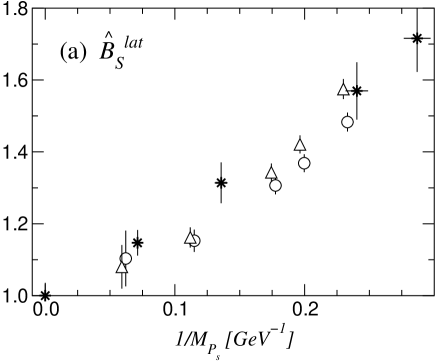
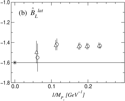
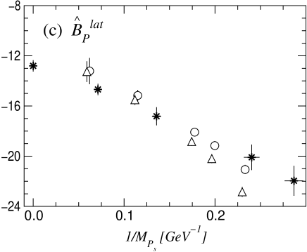
FIG. 1.: $1/M_{P_{s}}$ dependence of (a) $\hat{B}_{S}^{\rm lat}$, (b) $\hat{B}_{L}^{\rm lat}$ (=$\hat{B}_{R}^{\rm lat}$), and (c) $\hat{B}_{P}^{\rm lat}$. The results with $O(p/m_{Q})$ accuracy (circles) are compared to those with $O(p^{2}/m_{Q}^{2})$ (triangles) accuracy. The vacuum saturation approximation is shown by crosses.

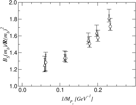
FIG. 2.: $1/M_{P_{s}}$ dependence of $B_{S}(m_{b})/{\cal R}(m_{b})^{2}$. Results with the $O(p/m_{Q})$ (circles) and $O(p^{/}m_{Q}^{2})$ (triangles) accuracies are shown. The smaller error bars represent statistical errors, while the uncertainties, obtained from a quadratic sum of the statistical uncertainty and difference between the central values with $\alpha_{V}(1/a)$ and $\alpha_{V}(\pi/a)$, are shown by the larger error bars. The central values are obtained with $\alpha_{V}(2/a)$.

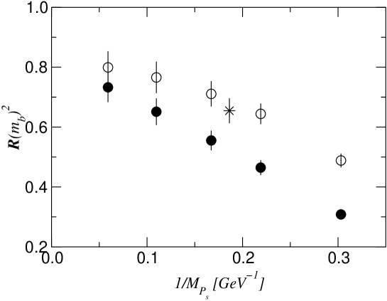
FIG. 3.: $1/M_{P_{s}}$ dependence of ${\cal R}(m_{b})^{2}$ evaluated with the method 1 (circles) and 2 (star). See the text for the detail. Open and filled symbols are obtained with and without the $1/(am_{Q})$ corrections in the one-loop coefficients.

REFERENCES

- [1] For a recent review, see for example, A.J. Buras and R. Fleischer, in Heavy Flavours II, eds A.J. Buras and M. Lindner, p.65, (World Scientific, Singapore, 1998).
- [2] I. Dunietz, Phys. Rev. D 52, 3048 (1995).
- [3] R. Fleischer and I. Dunietz, Phys. Lett. B 387, 361 (1996); Phys. Rev. D 55, 259 (1997).
- [4] M. Beneke, G. Buchalla and I. Dunietz, Phys. Rev. D 54, 4419 (1996).
- [5] M. Beneke, G. Buchalla, C. Greub, A. Lenz and U. Nierste, Phys. Lett. B 459, 631 (1999).
- [6] S. Hashimoto, K-I. Ishikawa, H. Matsufuru, T. Onogi, and N. Yamada, Phys. Rev. D 60, 094503 (1999).
- [7] S. Hashimoto, plenary talk presented at the XVII International Symposium on Lattice Field Theory (Lattice 99), Pisa, July, 1999, hep-lat/9909136.
- [8] R. Gupta, T. Bhattacharya, and S.R. Sharpe, Phys. Rev. D 55, 4036 (1997).
- [9] G.C. Branco, G.C. Cho, Y. Kizukuri, and N. Oshimo, Phys. Lett. B 337, 316 (1994); Nucl. Phys. B449, 483 (1995); D.A. Demir, A. Masiero, and O. Vives, Phys. Rev. Lett. 82, 2447 (1999).
- [10] B.A. Thacker and G.P. Lepage, Phys. Rev. D 43, 196 (1991); G.P. Lepage, L. Magnea, C. Nakhleh, U. Magnea, and K. Hornbostel, Phys. Rev. D 46, 4052 (1992).
- [11] B. Sheikholeslami and R. Wohlert, Nucl. Phys. B259, 572 (1985).
- [12] N. Yamada, S. Hashimoto, K-I. Ishikawa, H. Matsufuru, and T. Onogi, talk given at the XVII International Symposium on Lattice Field Theory (Lattice 99), Pisa, July 1999, hep-lat/9910006.
- [13] K-I. Ishikawa, T. Onogi, and N. Yamada, Phys. Rev. D 60, 034501 (1999).
- [14] E. Eichten and B. Hill, Phys. Lett. B 234, 511 (1990); Phys. Lett. B 240, 193 (1990).
- [15] K-I. Ishikawa, T. Onogi, and N. Yamada, talk given at the XVII International Symposium on Lattice Field Theory (Lattice 99), Pisa, July 1999, hep-lat/9909159.
- [16] A. Borrelli and C. Pittori, Nucl. Phys. B385, 502 (1992).
- [17] C.J. Morningstar and J. Shigemitsu, Phys. Rev. D 59, 094504 (1999).
- [18] G.P. Lepage and P.B. Mackenzie, Phys. Rev. D 48, 2250 (1993).
- [19] A. Borgland et al. (DELPHI collaboration), DELPHI 99-109 CONF 296, reported at EPS-HEP99.
- [20] K-I. Ishikawa et al. (JLQCD Collaboration), Phys. Rev. D 61, 074501 (2000).
- [21] K-I. Ishikawa, T. Onogi, M. Sakamoto, N. Tsutsui, N. Yamada, and S. Hashimoto, work in progress.
- [22] For example, see C. Caso et al. (Particle Data Group), Eur. Phys. J. C 3, 1 (1998).
- [23] M. Di Pierro and C.T. Sachrajda (UKQCD Collaboration), Nucl. Phys. B534, 373 (1998).
- [24] V. Giménez and J. Reyes, Nucl. Phys. B545, 576 (1999).
- [25] J. Flynn, O. Hernandez, and B. Hill, Phys. Rev. D 43, 3709 (1991).