Charm counting and $B$ semileptonic branching fraction

Abstract:

We review recent measurements as well as phenomenological background ofthe semileptonic branching fraction of $b$ hadrons and number of charm produced per decay of $b$ hadrons.

1 Introduction

The puzzle of inclusive non-leptonic $B$ decay was first pointed out in around 1994 [1, 2] when the theoretical prediction was considered to be difficult to accommodate 12% or less for the semileptonic branching ratio $B_{\rm s.l.}$ of $B$ meson while the measurement published by the CLEO collaboration was [3]

$$B_{\rm s.l.}=10.49\pm 0.46{\rm\%}\quad(\Upsilon(4S)).$$ (1)

The discrepancy was particularly stark when viewed in the two-dimensional plane of $n_{c}$ vs $B_{\rm s.l.}$, where $n_{c}$ is the average number of charm or anticharm created per $B$ decay [1, 2, 5]. The experimental value of $n_{c}$ was [4]

$$n_{c}=1.10\pm 0.05\,.$$ (2)

while the naive expectation was around 1.16. This was because when the uncertainties of the theory, in particular the charm quark mass, were tweaked to reduce $B_{\rm s.l.}$, it increased the inclusive non-leptonic decay rates which resulted in too large a value for $n_{c}$ compared to measurement. We have now new measurements related to this subjects which we will review below together with phenomenological background.

2 Definitions

By $B_{\rm s.l.}$, we mean the average branching fraction for direct electron production. The average is taken over the hadrons containing $b$ quark produced in a given environment. It is usually assumed that the electronic branching fraction is the same as the muonic branching fraction. In reality $B_{\rm s.l.}$ is average over weakly-decaying hadrons containing one $b$ quark. In the case of experiments running on the $\Upsilon(4S)$ resonance, the average is over $B^{+}$ and $B^{0}$ and their charge conjugate hadrons  produced nearly equal amount, and for the experiments running on $Z^{0}$, the average is taken over $B^{+}$, $B^{0}$, $B_{s}^{0}$, and baryons containing one $b$ quark which we denote as $N_{b}$. $N_{b}$ is in turn the mixture of $\Lambda_{b}(udb)$, $\Sigma_{b}(usb)$, $\Xi_{b}(dsb)$, and $\Omega_{b}(ssb)$. The relative fractions are roughly $B^{+}$:$B^{0}$:$B_{s}^{0}$:$N_{b}$ = 4:4:1:1; or more precisely [6]

$$\begin{array}[]{r@{\qquad\arrvsp}l}B^{+}\qquad\vspace{5 pt}&39.7^{+1.8}_{-2.2}{\rm\%}\\ B^{0}\qquad\vspace{5 pt}&39.7^{+1.8}_{-2.2}{\rm\%}\\ B_{s}^{0}\qquad\vspace{5 pt}&10.5^{+1.8}_{-1.7}{\rm\%}\\ N_{b}\qquad\vspace{5 pt}&10.1^{+3.9}_{-3.1}{\rm\%}\\ \end{array}$$

The charm count $n_{c}$ is the number of weakly-decaying charm or anticharm hadrons produced in the decay of one $b$-hadron, and it is again the average over the $b$-hadrons produced in the given environment. one usually counts the total number of $D^{+}$, $D^{0}$, $D_{s}^{+}$, $\Lambda_{c}$, $\Xi_{c}$. One exception is chamonium which is counted as two charms if it decayed by $c\bar{c}$ annihilation. Namely, a $J/\Psi$ meson produced in $b$-hadron decays are counted as two, while $\Psi^{\prime\prime}$ which decays predominantly to $D\bar{D}$ is counted when $D$ mesons are counted.

3 Theoretical tools

The basis of the predictions for $B_{\rm s.l.}$ and $n_{c}$ is the assumption is quark hadron duality which essentially states that the sum of rates to hadronic final states with a given flavor quantum number is the same as the sum of the rates at quark level to the same quantum numbers. There are two versions of this assumption: one is the global duality which applies to the case where the relevant rates are averaged over some range of c.m. energy. An example is the semileptonic decay of a $b$ hadron where the hadronic system in the final state can have different c.m. energies. Namely, in $b\to c\ell\nu$, the $c$ quark in the final state and the spectator quark that used to be in the parent $b$-hadron will form the hadronic system of the final state, and the c.m. energy of the system has a distribution over some range. The inclusive semileptonic rate is then estimated by taking the integration over it.

Another is the local duality where the rates of real hadronic final states are the same as the quark-level rates even if the c.m. energy of the hadronic system is fixed. This assumption is required to calculate the inclusive non-leptonic rates where all particles in the final states are hadrons. This is considered to be a stronger assumption than the global duality; since there are three quarks plus the spectator quark in the final state, however, one hopes that sufficient averaging over is involved to make the quark-level calculation reliable.

Then, the quark-level estimation is usually performed in the the heavy-quark expansion [7] and the perturbative QCD in the framework of the operator-product expansion [8]. The specific application starts with the optical theorem for the partial decay rate

$$\Gamma(B\to f) =$$

$${1\over m_{B}}{\rm Im}\langle B|i\int d^{4}xT({\cal L}_{\rm eff}(x)\hbox{\vrule height=10.0pt,depth=20.0pt,width=0.0pt}_{\makebox[0.0pt]{\hss$\overbrace{\sum_{f}|f\rangle\langle f|}$\hss}}{\cal L}_{\rm eff}(0))|B\rangle\,.$$

After expansion in terms of $1/m_{b}$, one obtains

$$\Gamma(B\to f) = \Gamma_{0}\Big{[}a\Big{(}1+{\lambda_{1}\over 2m_{b}^{2}}+{3\lambda_{2}\over 2m_{b}^{2}}\Big{)}$$ (4)

$$b{\lambda_{2}\over m_{b}^{2}}+{\cal O}({1\over m^{3}_{b}})\Big{]}\,,$$

where $\Gamma_{0}=G_{F}^{2}m_{b}^{5}/192\pi^{3}$, and the coefficients $a,b$ contains the effect of phase space, the Wilson coefficients estimated by perturbative QCD, and the CKM factors. The parameters $\lambda_{1}$ and $\lambda_{2}$ incorporates non-perturbative effects. The parameter $\lambda_{1}$ corresponds to $-\langle\vec{p}_{b}^{2}\rangle$ where $\vec{p}_{b}$ is the fermi-motion momentum of the $b$ quark inside the hadron, and one can identify the factor $1+\lambda_{1}/2m_{b}^{2}$ as the time delation factor for the decaying $b$ quark. There is a large uncertainty associated with the definition as well as the estimation of $\lambda_{1}$ varying from 0 to $\sim-0.7$ GeV². However, the effect on the non-leptonic decay rate is less than 2 %. The chromo-magnetic effect is contained in the parameter $\lambda_{2}$ which can be reliably estimated from the splitting of $B^{*}$ and $B$ mesons:

$$\lambda_{2}={m_{B}^{*2}-m_{B}^{2}\over 4}\sim 0.12{\rm GeV}^{2}\,.$$ (5)

Overall perturbative effect included in $\lambda_{1,2}$ is less than a few %. There are, however, non-perturbative effects that are not included in $\lambda_{1,2}$ such as possible large final-state interactions in $b\to c\bar{c}s$ mode where the particles in the final state are moving quite slowly.

The semileptonic branching fraction is then estimated as

$$B_{\rm s.l.}={\Gamma_{\rm s.l.}\over 2.22\Gamma_{\rm s.l.}+\Gamma_{\rm had}}={1\over 2.22+r_{\rm had}}\,,$$ (6)

where the factor 2.22 accounts for the total rate of $\ell\nu X$ $(\ell=e,\mu,\tau)$ in unit of $\Gamma_{\rm s.l.}$ (1 for $e$, 1 for $\mu$, and 0.22 for $\tau$), and $r_{\rm had}$ is the total non-leptonic rate again in unit of $\Gamma_{\rm s.l.}$:

$$r_{\rm had}=r_{\bar{u}d}+r_{\bar{c}s}+r_{\rm rare}\,.$$ (7)

Here, $r_{\bar{u}d}$ ($r_{\bar{c}s}$) is the rate for the decays caused by $b\to c\bar{u}d^{\prime}$ ($b\to c\bar{c}s^{\prime}$) transitions where $d^{\prime}$ ($s^{\prime}$) is the appropriate Cabibbo mixture of $d$ and $s$ quarks, and $r_{\rm rare}$ includes all charmless hadronic decays including penguins and $b\to u$ transitions. The value of $r_{\rm rare}$ is estimated in the standard model to be [9, 10]

$$r_{\rm rare}=0.25\pm 0.10\,.$$ (8)

The decays caused by $b\to u\bar{c}s^{\prime}$ transition is not included in the above classifications, but it is quite small at around 0.4% branching fraction.

A complete next-to-leading calculation of $r_{\bar{u}d}$ has been performed [11] which gives

$$r_{\bar{u}d}=4.0\pm 0.4\,,$$ (9)

where naively we expect $3$ for the color factor. The uncertainties involved are the renormalization scale $\mu$, quarks masses $m_{c}$ and $m_{b}$, and the assumption of quark hadron duality. The quark masses are constrained by the heavy-quark expansion relation

$$m_{b}-m_{c} = m_{B}-m_{D}$$ (10)

$$+\;{\lambda_{1}+3\lambda_{2}\over 2}\Big{(}{1\over m_{b}}-{1\over m_{c}}\Big{)}+{\cal O}({1\over m_{b}^{3}})$$

$$\sim 3.40\pm 0.06{\rm GeV}\,.$$

Thus, in the following, it is understood that changing $m_{b}$ will change $m_{c}$ accordingly. The value of $r_{\bar{u}d}$ as a function of $\mu/m_{b}$ is shown in the figure LABEL:fg:rud for $m_{b}=4.5$ GeV.

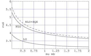
Figure 1: The estimate of $r_{\bar{u}d}$ for LO, NLO, and NLO + HQE estimations.

One notes that there is a substantial difference between the leading order (LO) estimation and the next-to-leading (NLO) estimation, and that the scale dependence of the NLO is not much better than that of LO. Both features are not encouraging with respect to the reliability of the final number. The correction due to the nonperturbative effects that are within the framework of the heavy-quark expansion (HQE) are small as mentioned earlier.

The uncertainty associated with the estimation of $r_{\bar{c}s}$ is generally considered to be larger than that for $r_{\bar{u}d}$. It is more sensitive to the quark masses and it was realized that there is a large QCD correction with finite charm quark mass due to a hard gluon emission from one the charm quarks in the final state [12, 13]. The correction enhanced the rate by about 30%. Also, the slow velocity of charm quarks makes it susceptible to final-state interactions [5].

Since the $b\to c\bar{u}s^{\prime}$ mode has one charm, the $b\to c\bar{s}^{\prime}$ has two charms, and the ’rare’ mode has no charm, the number of charm per $B$ decay $n_{c}$ is given by

$$n_{c} = 1+Br_{\bar{c}s}-Br_{\rm rare}$$ (11)

$$= 1+{r_{\bar{c}s}-r_{\rm rare}\over 2.22+r_{\rm had}}\,.$$

The theoretical values for $B_{\rm s.l.}$ and $n_{c}$ are [14]

$$\begin{array}[]{c@{\arrvsp}cc}\mu/m_{b}\hfil\vspace{5 pt}&1&1/2\cr B_{\rm s.l.}({\rm\%})\hfil\vspace{5 pt}&12.0\pm 1.0&10.9\pm 1.0\cr n_{c}\hfil\vspace{5 pt}&1.20\pm 0.06&1.21\pm 0.06\cr\end{array}$$ (12)

The quark masses used is $m_{c}/m_{b}=0.29$ or equivalently $m_{b}\sim 4.8$ GeV. It is seen that when $\mu$ is decreased $B_{\rm s.l.}$ goes down while $n_{c}$ is relatively stable; on the other hand, as $m_{c}/m_{b}$ is reduced $b\to c\bar{c}s^{\prime}$ rate increases with respect to $\Gamma_{\rm s.l.}$ and as the result $B_{\rm s.l.}$ goes down and $n_{c}$ goes up. If we would like to do away with the uncertainty in the $b\to c\bar{c}s^{\prime}$ mode, one could eliminate $r_{\bar{c}s}$ from the expression of $B_{\rm s.l.}$ and $n_{c}$ and obtain

$$n_{c}=2-(2.22+r_{\bar{u}d}+2r_{\rm rare})B_{\rm s.l.}\,,$$ (13)

which is a linear relation between $n_{c}$ and $B_{\rm s.l.}$ and the dominant error is that in $r_{\bar{u}d}$ if we are to trust the standard estimation of $r_{\rm rare}$. Using the values for $B_{\rm s.l.}$ (1), $r_{\bar{u}d}$ (9), and $r_{\rm rare}$ (8), $n_{c}$ becomes $1.30\pm 0.06$ which is to be compared with $1.10\pm 0.05$ (2). This 2.5 $\sigma$ discrepancy largely prompted proposals of new physics that boosts $r_{\rm rare}$ [1, 2, 15].

Sizes of corrections that affect $B_{\rm s.l.}$ and $n_{c}$ are shown in the table 1.

	naive	NLO($m_{c}=0$)	NLO($m_{c}\not=0$)
$r_{\ell\nu}$	2.22	2.22	2.22
$r_{\bar{u}d}$	3.0	4.0	4.0
$r_{\bar{c}s}$	1.2	1.6	2.1
$B_{\rm s.l.}$	0.16	0.13	0.12
$n_{c}$	1.16	1.17	1.21
$Br_{\rm cs}$	0.18	0.20	0.25

Table 1: Effects of various corrections affecting $B_{\rm s.l.}$ and $n_{c}$.

After all the corrections, the theoretical value of $B_{\rm s.l.}$ has come down and more or less consistent with the measurement. However, it is accomplished by boosting $r_{\bar{c}s}$ and it increased the estimation of $n_{c}$.

4 Measurements of $B_{\rm s.l.}$

On $\Upsilon(4S)$, the state-of-the-art is the correlated di-lepton method [16] where one $B$ is tagged by a high-momentum lepton and a lepton is searched for on ‘the other side. This allows one to separate the direct $b\to\ell^{-}$ from the cascade $b\to c\to\ell^{+}$ using the charge correlation of the tagged-side lepton and the signal-side lepton. This reduces the model dependence due to the subtraction of the cascade component. The effect due to the $B^{0}-\bar{B}^{0}$ mixing can be unfolded in each momentum bin by solving

$$\begin{array}[]{rl}{dN_{+-}\over dp}&=N_{\ell}\epsilon\left[{dB_{b}\over dp}(1-\chi)+{dB_{c}\over dp}\chi\right]\vspace{5 pt}\\ {dN_{\pm\pm}\over dp}&=N_{\ell}\epsilon\left[{dB_{b}\over dp}\chi+{dB_{c}\over dp}(1-\chi)\right]\end{array}$$ (14)

where $\chi=0.080\pm 0.012$ is the mixing parameter, $N_{+-}$ ($N_{++}$) is the observed number of opposite-sign (same-sign) dileptons, $N_{\ell}$ is the total number of tagging leptons, $\epsilon$ is the lepton detection efficiency, and $dB_{b}/dp$ ($dB_{c}/dp$) is the direct (cascade) lepton spectrum from $B$. The measurement (1) was made with this technique. The spectra thus obtained is shown in the figure 2.

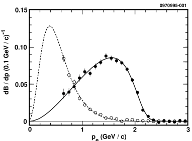
Figure 2: Unfolded spectra for direct (black circles) and cascade leptons (open circles) by the CLEO collaboration.

In principle, the leptons from the wrong-sign cascade $b\to\bar{c}\to\ell^{-}$, which can occur through $b\to c\bar{c}s$ where the $c\bar{c}$ pair fragment to $D\bar{D}_{(s)}X$, can contaminate the direct lepton sample. The momentum of such leptons, however, is low enough that the effect was found to be negligible.

The table 2 shows recent dedicated measurements of $B_{\rm s.l.}$ on the $Z^{0}$ peak. Values of $B_{\rm s.l.}$ obtained in global fits to electro-weak parameters are not included in this list.

Experiment	$B_{\rm s.l.}$(%)
ALEPH 95 [17]	$11.01\pm 0.10\pm 0.30$
L3 96 [18]	$10.68\pm 0.11\pm 0.46$
OPAL 99 [19]	$10.83\pm 0.10\pm 0.20^{+0.20}_{-0.13}$
DELPHI 99 [20]	$10.65\pm 0.07\pm 0.25^{+0.28}_{-0.12}$

Table 2: Recent measurements of $B_{\rm s.l.}$ at LEP. The model dependence is separated out as the last error for OPAL and DELPHI.

The Aleph analysis used a charge correlation method similar to the CLEO measurment above while single lepton sample was also used.

Figure 3: The $p_{T}$ pectra for direct and cascade leptons by the ALEPH collaboration.

The lepton spectrum obtained by ALEPH is shown in the figure 3. The spectrum is shown as functions of $p_{T}$ with respect to jet axis, and this makes the analysis sensitive to the contamination from the wrong-sign cascade $b\to\bar{c}\to\ell^{-}$.

The measurement by the L3 collaboration [18] combines separate measurements of $b\to e\nu X$, $\mu\nu X$, and $\nu X$. The neutrino mode is detected by large missing energy. The final number for $B_{\rm s.l.}$ is then obtained by a fit to the three samples. Charge correlations are not used.

The $B_{\rm s.l.}$ measurement reported by OPAL [19] begins by enhancing $Z^{0}\to b\bar{b}$ events by a lifetime flavor tagging technique based on neural net. The $b$-hemisphere sample is thus selected with a purity of 92% and an efficiency of 30%. Lepton is searched in the jet opposite to the tagged side. Two neural net variables $NN_{b\ell}$ and $NN_{bc\ell}$ are formed using $(p,p_{T})$ of the lepton, energy of the lepton-side jet, charge correlation of the lepton and the jet containing the lepton and that of the lepton and the most energetic jet on the tagging side, and impact parameter of the lepton. Also, the energy of the subjet containing the lepton is also used to enhance the sensitivity to $b\to c\to\ell^{+}$, and the scalar sum of $p_{T}$ of the lepton jet is used to enhance the sensitivity against light quark jets. Then, a maximum likelihood fit is performed on $NN_{b\ell}$ and $NN_{bc\ell}$ to extract number of direct leptons and cascade leptons.

Figure 4: The result of maximum likelihood fit to the neural net variable $NN_{bl}$ by the OPAL collaboration.

The result of the fit is shown in the figure 4. There are substantial difference in distribution shape for the three components which allows the separation among them. In addition to the direct $b\to\ell$ branching fraction, the fit also gives the cascade lepton branching ratio:

$$Br(b\to c\to\ell^{+})=8.40\pm 0.16\pm 0.21^{+0.33}_{-0.29}{\rm\%}\,.$$ (15)

Both for $B_{\rm s.l.}$ in the table as well as in the above, the last error represents model dependencies since the fit does require the lepton spectra for $b\to\ell$ and $b\to c\to\ell$ as well as fragmentation functions. The inclusion of the charge correlations in the fit, however, reduces the systematic error due to model dependences.

The DELPHI collaboration has combined four independent analyses:

1. The traditional single lepton counting on the opposite side to a hemisphere $b$-tagged by vertexing and lepton without charge correlation, plus di-lepton sample with charge correlation. Fitting the $(p,p_{T})$ distribution of the lepton(s), $B_{\rm s.l.}$ is extracted as

   $$B_{\rm s.l.}=10.66\pm 0.11\pm 0.24^{+0.25}_{0.12}{\rm\%}\,.$$ (16)

2. The $b$-hemisphere is tagged by vertexing and lepton on the opposite side, then two parameters are formed:

   $$\begin{array}[]{rcl}\lambda_{Q}&=&(\hbox{tag-side jet charge})\\ &&\times(\hbox{lepton charge})\vspace{5 pt}\\ k^{*}&=&p_{\rm lepton}\hbox{in the c.m. of $b$-hadron}\end{array}$$

   The $b$ vertex information is used to move to the c.m. of the $b$-hadron in order to obtain the absolute lepton momentum there since it has better separation power than $p_{T}$ for the cascade leptons. Then, a fit to the $(\lambda_{Q},k^{*})$ distribution gives

   $$B_{\rm s.l.}=10.74\pm 0.13\pm 0.41^{+0.46}_{0.30}{\rm\%}\,.$$ (17)

3. The analysis uses all hadronic events and employ a multi-variate method to separate flavors in which $(p,p^{\rm in}_{T},p_{T}^{\rm out})$ of leptons are reconstructed for each flavor where $p^{\rm in}_{T},p_{T}^{\rm out}$ are the $p_{T}$ with and without the lepton in calculating the jet axis. The result is

   $$B_{\rm s.l.}=10.64\pm 0.11\pm 0.25^{+0.37}_{-0.44}{\rm\%}\,.$$ (18)

4. In this analysis, the $b$ vertex is identified and then the charge of $b$ is determined by a neural net using jet charges and charged kaons etc. Then, the lepton momentum in the $b$-hadron c.m. system is fit separately for two relative charges of leptons giving

   $$B_{\rm s.l.}=10.81\pm 0.12\pm 0.26^{+0.35}_{-0.52}{\rm\%}\,.$$ (19)

The value of $B_{\rm s.l.}$ in the table is the combined result of the four measurements above where correlations among the measurements are taken into account. Also obtained are

$$Br(b\to c\to\ell^{+}) = 7.88\pm 0.13\pm 0.27^{+0.38}_{-0.32}{\rm\%}$$

$$Br(b\to c\to\ell^{-}) = 1.71\pm 0.13\pm 0.36^{+0.25}_{-0.19}{\rm\%}$$

Averaging the $B_{\rm s.l.}$ values of the four LEP experiments, the $B_{\rm s.l.}$ on $Z^{0}$ is

$$B_{\rm s.l.}=10.79\pm 0.17{\rm\%}\quad(Z^{0})\,.$$ (20)

5 Charm counting

There have been two types of charm counting reported so far. One way is to use the vertex information without explicitly reconstructing exclusive charm decays. The more traditional method is to exclusively reconstruct each charm hadrons. Recent results of the latter method are the CLEO result (2) and

$$n_{c}=\left\{\begin{array}[]{c}1.23\pm 0.036\pm 0.028\pm 0.053\\ \hbox{(ALEPH 96)}\\ 1.166\pm 0.031\pm 0.059\pm 0.054\\ \hbox{(DELPHI 99)}\\ \end{array}\right.\,,$$ (21)

measured on $Z^{0}$. The last error reflects the uncertainty in the branching fractions of charmed hadron decays. In the ALEPH analysis, the vertex $b$ tag was used to enhance $Z\to b\bar{b}$ events, and then the exclusive charm decays were counted. For DELPHI, the two sources of charm, $b\to c$ and $Z\to c\bar{c}$, were separated by the energy distribution of the charmed hadron and the vertex information, then the charm count was extracted using the measured value of $R_{b}$ which gives the total number of $Z\to b\bar{b}$ events. The breakdown the charm count is given in the table 3 together with results from OPAL which did not give the total count.

(%)	CLEO 96 [4]	ALEPH 96 [21]	OPAL 96 [22]	DELPHI 99 [23]
$D^{0}$	63.6$\pm$3.0	60.5$\pm$3.6	53.5$\pm$4.1	60.05$\pm$4.29
$D^{+}$	23.5$\pm$2.7	23.4$\pm$1.6	18.8$\pm$2.0	23.01$\pm$2.13
$D_{s}^{+}$	11.8$\pm$1.7	18.3$\pm$5.0	20.8$\pm$3.0	16.65$\pm$4.50
$\Lambda_{c}$	3.9$\pm$2.0	11.0$\pm$2.1	12.5$\pm$2.6	8.90$\pm$3.00
$\Xi_{c}^{0.+}$	2.0$\pm$1.0	6.3$\pm$2.1	$-$	4.00$\pm$1.60
$(c\bar{c})\times 2$	5.4$\pm$0.7	3.4$\pm$2.4	$-$	4.00$\pm$1.29

Table 3: Breakdown of charm counting by exclusive reconstruction of charm hadrons. Charmonia are indicated as $(c\bar{c})$. The CLEO result is the average over $B^{0}$ and $B^{+}$ while the LEP results are the average over $B^{0}$, $B^{+}$, $B_{s}$, and bottom baryons.

Some comments are in order. First, the CLEO result is the average over $B^{0}$ and $B^{+}$ while the LEP results are the average over $B^{0}$, $B^{+}$, $B_{s}$, and $N_{b}$ (bottom baryons). Thus one expects that the LEP results should have larger values for $D_{s}^{+}$ and charmed baryons; this is verified by the measurements.

Charmonia are indicated by $(c\bar{c})$ in the table, and it refers to the $c\bar{c}$ annihilating portion of $J\Psi$, $\Psi^{\prime}$, $\chi_{0,1,2}$, $\eta_{c}$, and $h_{c}$. Of which $J\Psi$, $\Psi^{\prime}$, and $\chi_{1}$ are actually detected, and theoretical prediction is used for $\eta_{c}$. If factorization works, $\chi_{1}$ and $h_{c}$ are not expected to be produced by $V-A$ interaction. For $\chi_{c2}$, CLEO has used its own measurement $Br(B\to\chi_{c2})=0.23\pm 0.10$%. This ‘signal, however, is now gone; thus, the number in the table as well as (2) should be reduced by 0.0023 which, luckily, is not a big change.

For $\Xi_{c}$, ALEPH and DELPHI used the CLEO measurement of $Br(B\to\Xi_{c})$ and added $Br(\Lambda_{b}\to\Xi_{c})$ prediction by JETSET. However, the value used by ALEPH $Br(B\to\Xi_{c})=3.9\pm 1.5$% [24] is now superceded by $Br(B\to\Xi_{c})=2.0\pm 1.0$% [24] which is used correctly by DELPHI. The older value was based on the assumption that the semileptonic rate of $\Xi_{c}$ is the same as that of $D$ which, together with the measured $\Xi_{c}$ lifetime, gave the branching fraction of the hadronic mode used in the detection of $\Xi_{c}$. However, the interference of the spectator $s$ quark and the $c\to s$ transition was found to substantially enhance the semileptonic decay rate of $\Xi_{c}$ [25]. The change in $Br(B\to\Xi_{c})$ largely reflects this correction. The CLEO value of $n_{c}$ and that in the table as well as the DELPHI values already include this correction. The ALEPH number, however, needs to be reduced; the corrected number is

$$n_{c} = 1.211\pm 0.036\pm 0.035\pm 0.053$$ (22)

$$\quad\hbox{(ALEPH, $\Xi_{c}$ corrected)}\,.$$

If we add the DELPHI values for $(c\bar{c})$ and $\Xi_{c}$ to the OPAL measurements for the rest of charmed hadrons, we obtain

$$n_{c} = 1.14\pm 0.06\pm 0.05$$ (23)

$$\hbox{(OPAL+$\Xi_{c},(c\bar{c})$ by DELPHI)}\,.$$

The branching fractions of $D^{0}$, $D^{+}$, and $D_{s}^{+}$ used in the charm counting are all normalized to $Br(D^{0}\to K^{-}\pi^{+})$. Thus, about 90% of $n_{c}$ is controlled by it; namely, $n_{c}$ is roughly inversely proportional to the value of $Br(D^{0}\to K^{-}\pi^{+})$ used in the analyses. The 1996 particle data group value is $Br(D^{0}\to K^{-}\pi^{+})=3.83\pm 0.12$%. Even though the uncertainty is included in the systematic errors stated, it is worthwhile to examine this number in some detail. There is a new precise measurement by ALEPH [26] tagging $D^{*+}\to D^{0}\pi^{+}$ by the $p_{T}$ of the slow pion in jet, which gave

$$Br(D^{0}\to K^{-}\pi^{+})=3.897\pm 0.094\pm 0.117{\rm\%}\,.$$

This is the method used by previous dominant measurements of the quantity. A slightly different technique was employed by CLEO where the mode $B\to D^{*+}\ell\nu$ was used to tag $D^{0}$. This requires reconstruction of $B\to D^{*+}\ell\nu$ using the lepton and the slow pion from $D^{*+}$ only. The figure 5 shows the recoil mass distribution of $\ell\pi$ pair for right-sign and wrong-sign samples. There is a clear signal for the right-sign combinations.

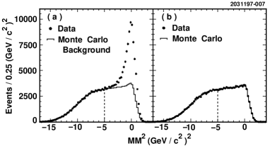
Figure 5: The recoil mass distribution of $B\to D^{*+}\ell\nu$ where the lepton and the soft pion only are detected. The right-sign [wrong-sign] $\ell\pi$ pairs are shown in (a) [(b)].

The result was

$$Br(D^{0}\to K^{-}\pi^{+})=3.81\pm 0.15\pm 0.16{\rm\%}\,.$$

These numbers are consistent with each other and there does not seem to be a big problem in $Br(D^{0}\to K^{-}\pi^{+})$. There is also a CLEO measurement [28] of $Br(D^{0}\to K^{-}\pi^{+})$ by requiring that $B\to X\ell\nu$ is saturated by the flavor-specific $D^{0,+}$ production apart from $b\to u\ell\nu$ and $b\to D_{s}^{+}X\ell\nu$ with the result $Br(D^{0}\to K^{-}\pi^{+})=3.69\pm 0.20$%. Since this number is obtained by forcing the charm counting in semileptonic sector to come out correct, it is not suited to use in the charm counting in general.

Another way to count the number of charm in $b$ decay is to extract it from the vertex information. This has an advantage of not dependent on the measured values of charm decay branching fractions. One such analysis was performed by DELPHI [29] where the $b$ vertex tag was used and the vertex information in the opposite side was used to form the probability that all tracks with positive lifetimes come from the primary vertex ($P^{+}_{H}$). Then, the distribution of $-\log P^{+}_{H}$ was fit with monte-carlo shapes of $b\to 0c$, $1c$, and $2c$ samples together with the $Z^{0}\to udsc$ backgrounds. The $-\log P^{+}_{H}$ distribution for the 1994 data and the result of the fit is shown in the figure 6.

Figure 6: Fit to the $-\log P^{+}_{H}$ distribution (1994 data) by $b\to 0c$, $1c$, $2c$, and background, where $P^{+}_{H}$ is the probability that all tracks with positive lifetimes come from the primary vertex.

The double charm and no-charm branching fraction thus obtained are

$$Br_{2c} = 0.136\pm 0.042\,,$$

$$Br_{0c} = 0.033\pm 0.021\,.$$

The zero-charm value includes the hidden-charm contribution $Br_{c\bar{c}}$ of charmonia decays estimated to be $0.026\pm 0.004$ which leaves

$$Br_{\rm rare}=0.007\pm 0.021$$

as the ‘rare’ branching fraction. This should be compared to the standard model prediction of $r_{\rm rare}B_{\rm s.l.}=0.026\pm 0.011$. The total number of charm was then estimated using $Br_{2c}$ only as

$$n_{c} = 1+Br_{2c}+Br_{c\bar{c}}-r_{\rm rare}B_{\rm s.l.}$$

$$= 1.147\pm 0.041\pm 0.008\,,$$

where $r_{\rm rare}B_{\rm s.l.}=0.016\pm 0.08$ was used.

6 Comparison of theory and experiment

We will take (20) as $B_{\rm s.l.}$ at $Z^{0}$ and convert it to $\Upsilon(4S)$ value by multiplying $\tau_{B}/\tau_{b}$:

$$B_{\rm s.l.}=11.07\pm 0.19\quad(Z^{0},\hbox{corrected})\,.$$

For $B_{\rm s.l.}$ on $\Upsilon(4S)$, we use the 1998 particle data group value:

$$B_{\rm s.l.}=10.45\pm 0.21{\rm\%}\quad(\Upsilon(4S))\,.$$ (24)

The discrepancy in $B_{\rm s.l.}$ between the $Z^{0}$ value and the $\Upsilon(4S)$ value is then 2.2 $\sigma$.

For $n_{c}$ at $Z^{0}$, we will first take the average of the ALEPH result corrected for $\Xi_{c}$ (22), the OPAL result supplemented by DELPHI numbers for $\Xi_{c}$ and charmonia (23), and the DELPHI result (21) to obtain

$$n_{c}=1.178\pm 0.035\pm 0.054\quad(Z^{0},{\rm exclusive})\,,$$ (25)

where the last error is due to charm decay branching fractions. Taking the average of this and the measurement using vertex information (5), we finally get

$$n_{c}=1.16\pm 0.04\quad(Z^{0})\,.$$ (26)

The results are shown in the figure 7 together with

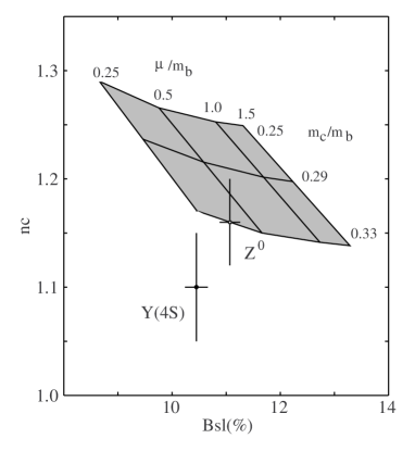
Figure 7: Comparison of experiment and theory for $B_{\rm s.l.}$ and $n_{c}$. The measurement on $Z^{0}$ and those on $\Upsilon(4S)$ are shown separately. The value of $B_{\rm s.l.}$ on $Z^{0}$ is corrected to correspond to the average of $B^{0}$ and $B^{+}$.

the theoretical expectation [14]. Compared to a few years ago, the $Z^{0}$ values have moved slightly toward the $\Upsilon(4S)$ values both in $B_{\rm s.l.}$ and $n_{c}$. The discrepancy between the measurements on $Z^{0}$ and those on $\Upsilon(4S)$ is still uncomfortable. If one takes the measurement on $\Upsilon(4S)$, the discrepancy between experiment and theory is alarming, and such discrepancy would be eliminated if we assume enhanced $r_{\rm rare}$ beyond the value of the standard model which would decrease the theoretical prediction of $B_{\rm s.l.}$ and also decrease that of $n_{c}$. If one takes the $Z^{0}$ values, however, the experiment and theory are consistent.

- [1] I.I. Bigi, B. Blok, M.A. Shifman, and A. Vainstein, Phys. Lett. B 323 (408) (1994).
- [2] A.F. Falk, M.B. Wise, and I. Dunietz Phys. Rev. D 51 (1183) (1995).
- [3] B. Barish et al. (CLEO collaboration), Phys. Rev. Lett. 76 (1570) (1996).
- [4] L. Gibbons et al. (CLEO collaboration), Phys. Rev. D 56 (3783) (1997).
- [5] I. Dunietz, J. Incandela, F.D. Snyder, and H. Yamamoto, Eur. Phys. J. C 1 (211) (1998).
- [6] Particle Data Group, Eur. Phys. J. C 3 (41) (1998). C3, 41 (1998).
- [7] M. Neubert, Phys. Rept. 245 (259) (1994) and references therein.
- [8] K. Wilson, Phys. Rev. 179 (1449) (1969); Phys. Rev. D 3 (1818) (1971).
- [9] G. Buchalla, I. Dunietz, and H. Yamamoto, Phys. Lett. B 364 (188) (1995).
- [10] H. Simma, G. Eilam, and D. Wyler, Nucl. Phys. B 352 (367) (1991).
- [11] E. Bagan, P. Ball, V.M. Braun, P. Gosdzinsky, Nucl. Phys. B 432 (3) (1994).
- [12] E. Bagan, P. Ball, V.M. Braun, P. Gosdzinsky, Phys. Lett. B 342 (362) (1995); [Erratum: Phys. Lett. B 374 (363) (1996)]; E. Bagan, P. Ball, B. Fiol, P. Gosdzinsky, Phys. Lett. B 351 (546) (1995).
- [13] M.B. Voloshin, Phys. Rev. D 51 (3948) (1995).
- [14] M. Neubert, C.T. Sachrajda, Nucl. Phys. B 483 (339) (1997).
- [15] B. Grzadkowski and W.-S. Hou, Phys. Lett. B 272 (383) (1991); A.L. Kagan, Phys. Rev. D 51 (6196) (1995); L. Roszkowski and M. Shifman, Phys. Rev. D 53 (404) (1996).
- [16] H. Albrecht et al. (ARGUS collaboration), Phys. Lett. B 318 (397) (1993).
- [17] The ALEPH collaboration, EPS95 conference reference, eps0404.
- [18] M. Acciarri et al. (L3 Collaboration) Z. Physik C 71 (379) (1996).
- [19] The OPAL collaboration, CERN preprint CERN-EP/99-078 (1999), submitted to Eur. Phys. J. C.
- [20] The DELPHI collaboration, Paper submitted to the HEP’99 Conference, Tampere, Finland, DELPHI 99-111 CONF 298 (1999).
- [21] D. Buskulic et al. (ALEPH collaboration), Phys. Lett. B 388 (648) (1996).
- [22] G. Alexander et al. (OPAL collaboration), Z. Physik C 72 (1) (1996).
- [23] The DELPHI collaboration, CERN preprint CERN-EP/99-66 (1999), submitted to Eur. Phys. J. C.
- [24] J.P. Alexander et al. (CLEO collaboration), Phys. Rev. Lett. 74 (3113) (1995); Errata: Phys. Rev. Lett. 75 (4155) (1995).
- [25] M.B. Voloshin, Phys. Lett. B 385 (369) (1996).
- [26] R. Barate et al. (ALEPH collaboration), Phys. Lett. B 403 (367) (1997).
- [27] M. Artuso et al. (CLEO collaboration), Phys. Rev. Lett. 80 (3193) (1998).
- [28] T.E. Coan et al. (CLEO collaboration), Phys. Rev. Lett. 80 (1150) (1998).
- [29] P. Abreu et al. (DELPHI collaboration), Phys. Lett. B 426 (193) (1998).