Report of the Beyond the Standard Model Working Group of the 1999 UK Phenomenology Workshop on Collider Physics (Durham)333To appear in Journal of Physics G
Abstract
The Beyond the Standard Model Working Group discussed a variety of topics relating to exotic searches at current and future colliders, and the phenomenology of current models beyond the Standard Model. For example, various supersymmetric (SUSY) and extra dimensions search possibilities and constraints are presented. Fine-tuning implications of SUSY searches are derived. The implications of Higgs (non)-discovery are discussed, as well as the program HDECAY. The individual contributions are included seperately. Much of the enclosed work is original, although some is reviewed.
Abstract
We re-analyse the best SUGRA discovery channel at the LHC, in order to re-express coverage in terms of a fine-tuning parameter and to extend the analysis to higher TeV. Such high values of have recently been found to have a focus point, leading to relatively low fine-tuning. It is found that even for as high as 3 TeV, mSUGRA can still be discovered for GeV. For GeV and (corresponding to the focus point), all points in mSUGRA with a fine tuning measure up to 220 are covered by the search.
Abstract
We discuss fine-tuning constraints on supergravity models. The tightest constraints come from the experimental mass limits on two key particles: the lightest CP even Higgs boson and the gluino. We also include the lightest chargino which is relevant when universal gaugino masses are assumed. For each of these particles we show how fine-tuning increases with the experimental mass limit, for four types of supergravity model: minimal supergravity, no-scale supergravity (relaxing the universal gaugino mass assumption), D-brane models and anomaly mediated supersymmetry breaking models. Among these models, the D-brane model is less fine tuned.The experimental prospects for an early discovery of Higgs and supersymmetry at LEP and the Tevatron are discussed in this framework.
Abstract
The properties of gluinonium are briefly reviewed. We then discuss possibilities for detection at run II of the Tevatron via peaks in the di-jet invariant mass spectrum.
Abstract
We discuss possible experimental signatures and distinctions between two models with extra dimensions. In the first model a number of large extra dimensions is postulated, while the second involves the addition of only one extra dimension, but with a metric which is non-factorisable into 4+1 separate dimensions (Randall-Sundrum model).
Abstract
A number of potential new physics processes can give rise to events containing isolated charged leptons and missing at LEP2. Most attention in this field has been focussed on the pair production of equal mass particles, which leads to events containing two leptons of roughly equal momenta. In this report we discuss potential new physics processes with the following experimental signatures: (i) events containing two leptons of unequal momenta; (ii) events containing a single visible lepton and no other activity in the detector.
Abstract
We briefly review precision electroweak fits, focussing upon their implications for the standard model Higgs mass. We review attempts to extend the analysis beyond the Standard Model in order to obtain information upon Higgs masses in a general scenario.
Abstract
We briefly review the effects of singlet scalars on the Higgs sector.
Abstract
The upper limit on the lightest -even Higgs boson mass, , is analysed within the MSSM as a function of for fixed and . The impact of recent diagrammatic two-loop results on this limit is investigated. We compare the MSSM theoretical upper bound on with the lower bound obtained from experimental searches at LEP. We estimate that with the LEP data taken until the end of 1999, the region can be excluded at the 95% confidence level. This corresponds to an excluded region within the MSSM for and TeV. The final exclusion sensitivity after the end of LEP, in the year 2000, is also briefly discussed. Finally, we determine the upper limit on within the Minimal Supergravity (M-SUGRA) scenario up to the two-loop level, consistent with radiative electroweak symmetry breaking. We find an upper bound of for in this scenario, which is slightly below the bound in the unconstrained MSSM.
Abstract
The program HDECAY determines the decay widths and branching ratios of the Higgs bosons within the Standard Model and its minimal supersymmetric extension, including the dominant higher-order corrections. New theoretical developments are briefly discussed and the new ingredients incorporated in the program are summarised.
1 Introduction
The ‘Beyond the Standard Model’ working group addressed the prospects for searches for supersymmetry, the phenomenology of large extra dimensions and the phenomenological implications of lower bounds upon the Higgs boson mass. The present status of large extra dimensions, SUSY breaking and searches for SUSY and leptoquarks were well covered in the plenary talks by G Ross and J Womersley.
There were three broad subgroups: Higgs phenomenology, SUSY breaking/large extra dimensions and the study of events containing isolated charged leptons and missing at LEP2. These subgroups had their own agendas of seminar presentations, discussions and reports. Summaries from each subgroup were given to the rest of the Beyond the Standard Model working group, and indeed the other working groups of the workshop. Much of the following work is original and carried out at the workshop, whereas some is the result of literature reviews.
The minimal supergravity (mSUGRA) reach potential of the LHC is readdressed in section 2. The exclusion limits are produced in terms of a naturalness parameter. In section 3, the fine-tuning implications of supersymmetric particle masses are presented in various SUSY breaking scenarios. The possibilities of detecting gluino-gluino bound states at run II of the Tevatron are examined in section 4. The experimental signatures and fits to current data of two models of extra dimensions are presented in section 5. In section 6, events containing isolated leptons and missing at LEP2 are discussed as a means of detecting, e.g., single chargino and production. Lower bounds upon the Higgs mass from LEP2 have been steadily increasing in the last two years, and the next sections address this empirical information. We present a review of what the precision electroweak fits imply once one retreats from the SM Higgs sector in section 7. Stealthy Higgs models that may be undetectable by the LHC are reviewed in section 8. State-of-the art upper limits upon the lightest Higgs boson mass in the general (R-parity conserving) MSSM and M-SUGRA are presented in section 9. Within the MSSM, using the most recent and prospective future LEP2 data, limits on are derived. Continuing work upon the Higgs decay program HDECAY was carried out at the workshop and the program is reviewed in section 10.
2 Naturalness Reach of the Large Hadron Collider in Minimal SUGRA
B C Allanach, J P J Hetherington, M A Parker, G G Ross, B R Webber
Recent work [1] has shown that MSSM scalar masses as large as 2 to 3 TeV can be consistent with naturalness. This occurs near a ‘focus point’ where the renormalisation group trajectories of the mass squared of a Higgs doublet () cross close to the electroweak scale. As a result, the electroweak symmetry breaking is insensitive to ultraviolet boundary conditions upon SUSY breaking parameters [1]. Previous predictions of the discovery reach of the LHC into mSUGRA parameter space went only as far as TeV [2]. The purpose of this work is to extend this reach to 3 TeV and to present it in terms of a naturalness measure. While interpretation of a naturalness measure is inevitably subjective, we advocate its use as a single parameter for defining the search reach of a collider in the context of a particular model. The naturalness coverage could then be used to compare between different colliders/experiments/models etc.
At tree-level, the boson mass is determined to be
| (1) |
by minimising the Higgs potential. refers to the ratio of Higgs vacuum expectation values (VEVs) and to the Higgs mass parameter in the MSSM superpotential. In mSUGRA, has the same origin as the super-partner masses (). Thus as search limits put lower bounds upon super-partners’ masses, the lower bound upon rises, and consequently so does . A cancellation is then required between the first and second terms of equation 1 in order to provide the measured value of . Various measures have been proposed in order to quantify this cancellation [4].
The definition of naturalness of a ‘fundamental’ parameter employed in reference [1] is
| (2) |
From a choice of a set of fundamental parameters , the fine-tuning of a particular model is defined to be . Our choice of free, continuously valued, independent and fundamental mSUGRA parameters also follows ref. [1]:
| (3) |
where GeV is the GUT scale.
We now turn to the discussion of the LHC mSUGRA search. In the ATLAS TDR [2] the best reach was found through a 1 lepton plus jets plus missing transverse momentum signal, which looks mainly for chargino decays to lepton and sneutrino. The following cuts were employed, which are the same as those as in refs. [2, 3] except where those original cuts are included in parenthesis:
-
•
GeV
-
•
At least 2 jets, with rapidity , and GeV.
-
•
1 lepton, , GeV, lying further in space than 0.4 units from the centre of any jet with cone-size 0.4 (0.7) (less than 5 GeV of energy within 0.3 units of the lepton).
-
•
(4) where , are transverse two-component lepton and missing respectively.
-
•
(5) where are the eigenvalues of the sphericity matrix , the sum being taken over all detectable final state particles, and being the two-component transverse momentum attributed to the cell.
mSUGRA events were simulated by employing the ISASUSY part of the ISAJET7.42 package [5] to calculate sparticle masses and branching ratios, and HERWIG6.1 [6] to simulate the events themselves. Fig. 1 shows the contour for 10 signal events passing the above cuts as a black line in the plane for mSUGRA with GeV, , GeV, and for fb-1 of luminosity (equivalent to a one year of running in the low luminosity mode). Background at regions of parameter space with such high energy cuts is estimated to be negligible. The discovery contour is overlaid upon the density of naturalness (displayed as background) as defined above. was calculated numerically to one-loop accuracy in soft masses, with two-loop accuracy in supersymmetric parameters and step-function decoupling of sparticles. Dominant one-loop top/stop corrections are added to the Higgs potential and correct equation 1. This approximation was also used to calculate the black (excluded) regions in figure 1. We note that the horizontal piece of the bottom black region results from the limit GeV, whereas the diagonal piece is from the constraint of electroweak symmetry breaking. This last constraint is very sensitive to , and moves to the right and off the plot for GeV. We note that while the naturalness contours displayed in Figure 1 are of the same shape as those calculated before [1], the fine tuning is some 50% higher. This is due [4] to the approximation of using an incomplete one-loop potential, and will be rectified [7] (as will the approximation of using constant over the plane).
References
References
- [1] J.L Feng et al, Phys. Rev.D61 (2000) 075005, hep-ph/9908309
- [2] ATLAS Collaboration, Detector and Physics Performance TDR, Volume II, Technical Report CERN/LHCC 99-15, (1999) CERN
- [3] H Baer et alPhys. Rev.D53 (1996) 6241
- [4] See for example R. Barbieri and A. Strumia, Phys. Lett.B433 (1998) 63; B. de Carlos and J.A. Casas, Phys. Lett.B320 (1993) 320
- [5] H. Baer et alhep-ph/9810440
- [6] HERWIG6.1 collaboration, http://home.cern.ch/seymour/herwig/herwig61.html, Cavendish-HEP-99/03
- [7] B.C. Allanach et alwork in progress
3 Fine-Tuning Constraints on Supergravity Models
M Bastero-Gil, G L Kane and S F King
When should physicists give up on low energy supersymmetry? The question revolves around the issue of how much fine-tuning one is prepared to tolerate. Although fine-tuning is not a well defined concept, the general notion of fine-tuning is unavoidable since it is the existence of fine-tuning in the standard model which provides the strongest motivation for low energy supersymmetry, and the widespread belief that superpartners should be found before or at the LHC. Although a precise measure of absolute fine-tuning is impossible, the idea of relative fine-tuning can be helpful in selecting certain models and regions of parameter space over others111For a complete list of references and a fuller discussion of these results see M. Bastero-Gil, G. L. Kane and S. F. King, hep-ph/9910506..
The models we consider, and the corresponding input parameters given at the unification scale, are listed below:
-
1.
Minimal supergravity
(6) where as usual , and are the universal scalar mass, gaugino mass and trilinear coupling respectively, is the soft breaking bilinear coupling in the Higgs potential and is the Higgsino mass parameter.
-
2.
No-scale supergravity with non-universal gaugino masses222This is in fact a new model not previously considered in the literature, although the no-scale model with universal gaugino masses is of course well known. As in the usual no-scale model, this model has the attractive feature that flavour-changing neutral currents at low energies are very suppressed, since all the scalar masses are generated by radiative corrections, via the renormalisation group equations, which only depend on the gauge couplings which are of course flavour-independent.
(7) -
3.
D-brane model
(8) where and are the goldstino angles, with , and is the gravitino mass. The gaugino masses are given by
(9) and there are two types of soft scalar masses
(10) -
4.
Anomaly mediated supersymmetry breaking
(11)
Our main results are shown in Figures 2-5, corresponding to SUGRA models 1-4 above. In all models, fine-tuning is reduced as is increased, with preferred over . Nevertheless, the present LEP2 limit on the Higgs and chargino mass of about 100 GeV and the gluino mass limit of about 250 GeV implies that is of order 10 or higher. The fine-tuning increases most sharply with the Higgs mass. The Higgs fine-tuning curves are fairly model independent, and as the Higgs mass limit rises above 100 GeV come to quickly dominate the fine-tuning. We conclude that the prospects for the discovery of the Higgs boson at LEP2 are good. For each model there is a correlation between the Higgs, chargino and gluino mass, for a given value of fine-tuning. For example if the Higgs is discovered at a particular mass value, then the corresponding chargino and gluino mass for each can be read off from Figures 2-5.
The new general features of the results may then be summarised as follows:
-
•
The gluino mass curves are less model dependent than the chargino curves, and this implies that in all models if the fine-tuning is not too large then the prospects for the discovery of the gluino at the Tevatron are good.
-
•
The fine-tuning due to the chargino mass is model dependent. For example in the no-scale model with non-universal gaugino masses and the D-brane scenario the charginos may be relatively heavy compared to mSUGRA.
-
•
Some models have less fine-tuning than others. We may order the models on the basis of fine-tuning from the lowest fine-tuning to the highest fine-tuning: D-brane scenario generalised no-scale SUGRA mSUGRA AMSB.
-
•
The D-brane model is less fine-tuned partly because the gaugino masses are non-universal, and partly because there are large regions where , , and are all close to zero However in these regions the fine tuning is dominated by , and this leads to an inescapable fine-tuning constraint on the Higgs and gluino mass.
4 Gluino-gluino bound states
V Kartvelishvili and R McNulty
If the decay of a gluino into a quark-squark pair is forbidden kinematically and parity is conserved, the gluino can only decay into a quark-antiquark pair an a neutralino, via a virtual squark, with a far longer lifetime. In this case the usual strategies for gluino searches using high jets and missing transverse energies are far less efficient — the jets are more numerous and hence softer, while the missing energy is smaller. Consequently, the reach for gluino searches is significantly reduced and it is quite difficult to obtain a model-independent limit.
In this case, however, there is a possibility of observing the gluino indirectly, by detecting a gluino-gluino bound state(see [1, 2] and references therein). This has the advantage that the conclusions which can be drawn from a search for such states hold in a very wide class of supersymmetry models. In addition, the detection of such a state would lead to a relatively precise determination of the gluino mass, which could not be obtained easily by observing the decay products of the gluino itself, as some of these escape undetected.
Gluino-gluino bound states (sometimes called gluinonium) can be detected as narrow peaks in the di-jet invariant mass distributions. The main problem is the high background from QCD high jets, and thus it is vital to have two-jet invariant mass resolution as good as possible.
4.1 Properties of gluinonium
As strongly interacting fermions, gluinos have a lot in common with heavy quarks. There are important differences though:
-
•
gluino has no electroweak coupling, so its lifetime is defined by its strong decays. For our case of interest, , this means that gluino lives long enough to form a bound state;
-
•
gluino is a colour octet; the potential between two gluinos is attractive not only if they are in a colour-singlet state, but also if they are in colour octet states, both symmetric and antisymmetric;
-
•
gluino is a Majorana fermion (i.e. is its own antiparticle), and some gluinonium states are forbidden due to the Pauli principle.
Table 1. Spin-parities for the allowed low lying states of gluinonium with . The three columns correspond to the colour singlet state 1 and the symmetric and antisymmetric colour octet states and respectively.
The resulting spectra of low-lying gluinonium states [3] are shown in Table 1. The allowed colour singlet 1 and symmetric octet states have the same values as the charmonium states with , while the allowed antisymmetric colour octet states have the same values as the charmonium states with . In particular, the lowest lying colour singlet and symmetric colour octet states are the pseudoscalars and with , while the lowest lying antisymmetric colour octet state is vector gluinonium with .
All three states decay via gluino-gluino annihilation. The pseudoscalars decay mainly to two gluons [3] with decay widths , while vector gluinonium decays predominantly into pairs [4] with a decay width about . Although much larger than the free gluino decay width, these widths are still very small compared to the gluinonium mass . The size of all three states is of order , which is much smaller than the confinement length, thus justifying the relative stability of the colour octet states (see [1, 4]).
So, the vector gluinonium is a heavy compact object which behaves rather like a heavy gluon, except that its coupling to quarks is much stronger than its coupling to gluons. Hence it is most readily produced via annihilation and the Tevatron is a promising place to look, being a source of both valence quarks and valence antiquarks. In contrast, the pseudoscalar states and couple predominantly to gluons, and can be produced equally well in both and collisions via the gluon-gluon fusion mechanism. Their production cross-section increases more rapidly with energy than that for vector gluinonium, and there is more chance of detecting them at the LHC.
4.2 Vector gluinonium at the Tevatron
The vector gluinonium is produced and decays in collisions via the subprocess
| (12) |
where we use the symbols and to distinguish light and heavy quarks333Obviously, -quarks contribute only if the gluino is heavy enough, and even then for the range of gluino masses accessible at the Tevatron this contribution is strongly suppressed by the available phase space..
The nature of the background depends on . At Tevatron energies, the range of interest lies mainly in large values , where the luminosity of colliding pairs prevails over that of gluon-gluon pairs. In this region, the main sources of two-jet background are the subprocesses
| (13) |
where the first two have the angular dependence , peaking sharply at , where is defined in c.m. frame of the two jets. In contrast, the signal from the subprocess (12) has a much weaker dependence, . Hence, a cut should improve the signal-to-background ratio.
The usefulness of heavy quark tagging is clearly brought out by considering the production ratios for the various final states in both the signal (12) and background (13). The relative contribution of the three background subprocesses in (13) at small is given by [4]
| (14) |
while for the signal (12) one has
| (15) |
Hence by tagging the heavy quark jets one reduces the background by a factor of , while retaining 40% of the signal.
At smaller gluinonium masses GeV, initial gluons contribute much more significantly to the background, even with heavy quark jet tagging, through the subprocess
| (16) |
This makes the signal-to-background ratio hopelessly small for any realistic di-jet invariant mass resolution. However, this region of gluino masses is already covered by other methods.
4.3 Simulation
So, most of the two-jet QCD background at large invariant masses arises from light quark and gluon jets, and the signal-to-background ratio can be significantly enhanced by triggering on heavy quark jets [4]. To check that this makes the detection of vector gluinonium a viable possibility at the upgraded Tevatron, we have simulated both the gluinonium signal and the 2-jet QCD background using PYTHIA 5.7. The vector gluinonium production and decay was simulated by exploiting the fact that behaves much like a heavy with axial current and lepton couplings set to zero and a known mass-dependent vector current coupling to quarks, chosen to comply with the corresponding decay width after taking into account appropriate colour and flavour counting. This effective coupling included the non-Coulomb corrections and an enhancement due to the fact that numerous radial excitations of the , which could not be separated from it for any reasonable mass resolution, will also contribute. These yield an overall factor of between 1.8 and 1.6 depending on , and the resulting effective vector coupling falls exponentially from at GeV to at GeV. This signal sits on a much larger background, which has been simulated on the assumption that it arises entirely from the leading order QCD subprocesses for heavy quark pair production (13) and (16). A constant factor has been used for both signal and background.
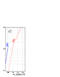
The cross section for vector gluinonium production at the upgraded Tevatron with its energy increased to 2 TeV is shown in Fig. 1. Only decays into heavy quark-antiquark pairs were taken into account, and the tagging efficiency for at least one - or -quark jet was assumed to be . The cut on the jet angle in the two-jet c.m frame was , and the cut on jet rapidity was . The signal-to-background ratio was found to be around at the peak for the assumed two-jet invariant mass resolutions of 25 GeV, 30 GeV and 38 GeV at GeV, 320 GeV and 450 GeV respectively. One can hope to see the gluinonium signal from gluinos with masses up to 220 GeV as a 5 standard deviation peak, and the signal from gluinos with masses up to 260 GeV as a 3 standard deviation peak. Note that the statistical significance of the peak is essentially inversely proportional to the two-jet invariant mass resolution, so the reach can be significantly extended if some way is found to improve the latter.
4.4 Conclusion
We conclude that gluinonium states can be detected as narrow peaks in the di-jet invariant mass spectra, effectively complementing more traditional gluino searches, in the case when the gluino is lighter than the squarks.
In collisions one expects copious production of vector gluinonium, which decays predominantly to pairs. The high efficiency of the heavy quark jet tagging together with the boost of the Tevatron energy and luminosity should allow one to reach gluino masses of 220-260 GeV at TeV and 1000 pb-1, with realistic efficiencies, resolutions and experimental cuts taken into account. It is crucial, however, to improve tagging efficiency for both and quark jets, as well as the two-jet invariant mass resolution for these jets.
References
References
- [1] H.R. Haber and G.L.Kane, Phys. Rep.117, 75 (1984).
- [2] E.Chikovani, V.Kartvelishvili, R.Shanidze and G.Shaw, Phys. Rev. D53, 6653 (1996).
- [3] W.Y. Keung and A. Khare, Phys. Rev. D29, 2657 (1984); J.H. Kühn and S. Ono, Phys. Lett. B142, 436 (1984); T. Goldman and H.E. Haber, Physica 15D, 181 (1985).
- [4] E.G. Chikovani, V.G. Kartvelishvili and A.V. Tkabladze, Z. Phys.C43, 509 (1989); Sov. J. Nucl. Phys.51 546, (1990).
5 Experimental Signatures from Theories with Extra Dimensions
J Grosse-Knetter, J Holt and S Lola
An important issue in extending the Standard Model of Particle Physics, is the hierarchy problem, arising from the existence of two vastly different fundamental scales ( and ). There are ways to evade this problem, such as technicolour and supersymmetry. A third solution which has recently received considerable attention, is to identify the Planck scale with the electroweak scale, by introducing extra dimensions into which gravitons are able to propagate. Here, we discuss some experimental aspects of two classes of such models.
5.1 Models with large Extra Dimensions
The first set of models considered here is the proposal of [1] where the Plank scale, , is related to the scale of gravitational interactions, in a space which includes extra compact dimensions of radius . In this case, one finds that [1], where is the number of the extra dimensions: for which is obviously excluded. However, already for , . No effects of the extra dimensions on Standard Model fields in accelerators have been observed, one therefore assumes that our 4-dimensional world lies on a brane while the gravitons (which feel the extra dimensions) can propagate on the bulk. Since momentum in extra dimensions is seen as mass in four dimensions, in computing graviton emission one has to sum over a tower of massive Kaluza-Klein states, with masses . The coupling to any single mode has the normal gravitational strength (, where ), while the mass of each mode is very small. However the large multiplicity of modes, given approximately by , where denotes the energy that is available to the graviton, increases the effective coupling dramatically.
The Feynman rules for the new vertices [2] are calculated from , where labels the Kaluza-Klein modes. Some features for the interactions that arise in this class of models, which are important for accelerator searches, are the following: (i) the interactions are flavour-independent. (ii) the individual modes are very light and couple very weakly, thus may not be produced on resonance. (iii) the spin-2 nature of the graviton can be determined via angular distributions of the cross sections. (iv) the effective coupling scales as and therefore a strong energy dependence (with increase of the cross sections as the energy increases) should appear.
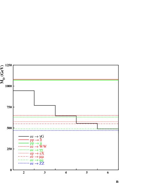
5.2 Limits on Models with Large Extra Dimensions
The effects of gravity in models with large extra dimensions, have been searched for using the data from a number of experiments in different channels. No evidence for these effects has been found and lower limits on the parameter , as a function of the number of extra dimensions, , have been obtained from the different sets of data. Some of these limits, taken from [3] together with the results presented below from HERA DIS, are shown in figure 7. The limits coming from at LEP II show a strong dependence on the number of extra dimensions. The cross-section for this process depends on the phase space available to the emitted gravitons which depends on . The other limits are derived from processes which involve virtual exchange of gravitons. The effective string scale has been taken to be equal to . The graviton exchange can interfere constructively or destructively with the Standard Model processes, set by a parameter ; the above limits are for
The best limits under these assumptions come from the TEVATRON from di-lepton production using a combination of CDF and D0 data. Limits from CDF alone on di-jet production are very competitive, suggesting that improved sensitivity could be obtained by including D0 di-jet data. Combining all the channels studied by L3 at LEP II, gives a lower limit on of 860 GeV [3] from approximately 50 of data. The four LEP collaboration now have a total of more than 1.6 worth of data collected at energies above GeV. Combining all results sensitive to virtual graviton exchange, from all four experiments, could give results which would compete with those from the TEVATRON.
5.3 Fits to HERA DIS data
One of the processes with sensitivity to effects predicted from Kaluza-Klein models with large extra dimensions is the neutral-current (NC) deep-inelastic scattering (DIS) of positrons off protons. Effects are expected through the exchange of gravitons coupling to both and in addition to the SM-exchange of photons and bosons [6]. These additional contributions (expected at large , lead to an enhancement in the cross section , where is the squared four-momentum transferred between positron and proton.
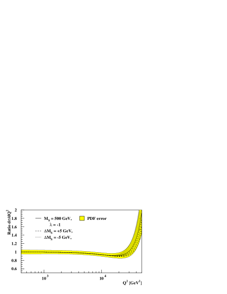
Fitting the cross section expected from the combination of the SM and graviton exchange to recent NC DIS data from ZEUS [7] (similar results are expected from corresponding H1 data [8]) using CTEQ4 PDFs yields CL limits of GeV ( and GeV ( in agreement with expectations based on preliminary data [6]. The results are illustrated in figure 8(a) as the ratio of fitted cross section to that expected from the SM.

It was further investigated whether the recent HERA NC DIS data [9] can provide additional information on the mass-scale of extra dimensions. For this purpose NC DIS data were simulated based on the uncertainty expected from the luminosity of the existing data sample. Fits similar to above were performed as shown in figure 8(b) yielding GeV ( and GeV (. Thus no stricter limits than already obtained from the data should be expected.
The predicted cross-sections for process at the TEVATRON and HERA, are sensitive to uncertainties in the parton distributions functions (PDFs) of the proton. We first estimate the uncertainties in arising from PDF uncertainties in fits to HERA DIS data. For this purpose results are used from a NLO QCD fit [7] to measurements of proton structure functions and quark asymmetries from collider and fixed target experiments. The fit propagates statistical and correlated systematic errors from each experiment to corresponding errors in the PDFs which are used to determine uncertainties in the cross section , including contributions from graviton exchange. The result is shown as ratio of (SM+graviton) for GeV and to (SM) in figure 9 (left). The band shows the uncertainty in the ratio (SM+graviton)/(SM) arising from PDF uncertainties. The latter was compared to the variation in the ratio as changes, for nominal PDFs. These are shown by the dashed and dotted lines, where incremental changes in of 5 GeV are made. This procedure shows that only small errors in , of approximately 15 GeV, arising from PDF uncertainties should be expected.

Similar effects from PDF uncertainties are expected for fits to TEVATRON data. To check the effect of PDF uncertainties on this limit the Drell-Yan cross section ( being the hard scale, ie the mass) is determined in leading-order QCD with two different PDF sets444The PDF uncertainties from the QCD fit described above were only available for hard scales corresponding to GeV, so below the range sensitive to graviton exchange and could thus not be used here. including contributions from graviton exchange, in figure 9 (right). This analysis indicates that uncertainties in the limits on resulting from PDF uncertainties should be expected to be of order 10 to 20 GeV.
5.4 Randall–Sundrum in at LEP II
So far, we have been referring to models with more than one extra dimensions and with a factorisable metric. One can instead envisage a case where a large mass hierarchy may be generated by an exponential “warped” factor of a small compactification radius, , in a case of a 5-dimensional non-factorisable geometry [4]. It turns out that a field with a fundamental mass parameter on the visible world appears to have a physical mass , where is a scale of order the Planck scale, relating the 5-dimensional Planck scale to the cosmological constant. The interaction Lagrangian in the 4-dimensional effective theory indicates that, while the zero mode couples with the usual 4-dimensional strength, the massive KK states are relatively unsuppressed. Thus, unlike the previous case of more than one factorisable extra dimension, now (i) the individual modes are heavier (). (ii) the individual modes couple with weak interaction strength thus may be produced on resonance. (iii) as one increases the centre of mass energy, one may hope to probe a multi-resonance effect.
For instance, for the first mode, the mass, and the width, , of the resonance are given by and where is the first non-zero root of the Bessel function and is a constant which depends on the number of decay channels. Moreover, by making the substitution in the formulas obtained for factorisable extra-dimensions, one can proceed to calculate any process. Clearly, as grows, the resonant peaks are substituted by a contact-interaction behaviour.

The possibility of finding a Randall-Sundrum resonance with a mass as low as 100-200 GeV in at LEP II has been investigated. It would be possible to hunt for such a resonance by examining the distribution of the number of muon events observed as a function of the invariant mass, , of the pair of muons, taking advantage of initial state radiation which provides access to invariant masses below the centre–of–mass energy of the LEP collision energy, .
Born–level predictions for the cross–section, , of the Randall–Sundrum model with GeV and are shown in figure 10. The mass of the first resonance is approximately 150 GeV. In principle the parameter which determines the width can be calculated. For the studies presented here was chosen so that the width of the first resonance was 1 GeV. The QED convoluted cross–section as a function of is given by . The radiator function, , was computed for bins of for the by computing the Born–level cross–section and in the Standard Model. This was then applied to the predictions including the Randall–Sundrum resonance. The QED convoluted cross-section for a centre–of–mass energy of 200 GeV is shown in figure 10(b). The predicted numbers of events figure 10(c), for a luminosity 200 . The distribution has been smeared to take into account the experimental resolution, which was obtained from a simulation of the DELPHI detector.
The difference between the the Randall–Sundrum Model and the Standard Model, , is shown in figure 10(d) in terms of the number of statistical standard deviation on the expected numbers of events. Even taking into account the resolution on , it is clear that a Randall–Sundrum resonance with the parameters given above would be observable at LEP II given 200 at GeV. In reality each of the LEP experiments have this much data collected at centre–of-mass energies between 192 and 202 GeV. The spread of energies should not significantly change the ability to observe such a resonance, or place limits in the () plane. A fit could include all centre of mass energies and all other final states in collisions sensitive to the presence of a Randall–Sundrum mode.
References
References
- [1] N. Arkani-Hamed, S. Dimopoulos and G. Dvali, Phys. Rev. D59 (1999) 086004.
- [2] G.F. Giudice, R. Rattazzi and J.D. Wells, Nucl. Phys. B544 (1999) 3.
- [3] L3 Collaboration, M Acciarri et al., Phys. Lett. B464 (1999) 135; P. Mathews et al., hep-ph/9904232 (1999); A.K. Gupta et al., hep-ph/9904234 (1999).
- [4] L. Randall and R. Sundrum, Phys. Rev. Lett. 83 (1999) 3370.
- [5] H. Davoudiasl, J.L. Hewett and T.G. Rizzo, hep-ph/9909255.
- [6] P. Mathews, S. Raychaudhuri and K. Sridhar, Phys. Lett. B455 (1999) 115.
- [7] ZEUS Collaboration, J. Breitweg et al., Eur. Phys. Jnl. C11 (1999) 427.
- [8] H1 Collaboration, C. Adloff et al., DESY 99-107 (1999), hep-ex/9908059.
- [9] H1 Collaboration, Abstract No 157b, presented at HEP99, Tampere, Finland, July 1999; ZEUS Collaboration, Abstract No 549, ibid.
- [10] CDF Collaboration, F. Abe et al., Phys. Rev. D59 (1999) 052002; D0 Collaboration, B. Abbott et al., Phys. Rev. Lett. 82 (1999) 4769.
6 Some Alternative Tests of Standard Supersymmetry with Events Containing Isolated Leptons and Missing at LEP2
D Hutchcroft, J Kalinowski, R McNulty, G Wilson, T Wyatt
In the Standard Model (SM), low multiplicity events containing charged leptons and significant missing transverse momentum, , arise from the final state . The most important SM process contributing to this final state is production in which both W’s decay leptonically: W (with ), thus producing events containing an “acoplanar”555The acoplanarity angle is defined as 180∘ minus the angle between the two lepton candidates in the plane transverse to the beam direction. pair of observed leptons. The SM subprocess leading to the final state W-e tends to produce events containing a single observed lepton, since the e+ has a high probability to be scattered at a small angle to the beam direction and thus escape detection.
Events containing charged leptons and are also an experimental signature for the production of new particles that decay to a charged lepton accompanied by one or more invisible particles. For example, acoplanar di-lepton events are a signal for the pair production of new particles such as:
- charged scalar leptons (sleptons):
-
, where may be a selectron (), smuon () or stau (), is the corresponding charged lepton and is the lightest neutralino.
- charged Higgs bosons:
-
.
- charginos:
-
(“2-body” decays) or (“3-body” decays).
A typical candidate event is shown in figure 11.
The LEP detectors provide hermetic detection for showering and minimum ionising particles, typically down to an angle of around 0.04 rad with respect to the beam direction. This means that the potential background from SM processes such as , which have four charged leptons in the final state (of which only two are observed in the detector), can be reduced to a low level. Such potential backgrounds do, however, mean that the scaled missing transverse momentum of selected events, /, has to be required to exceed around 0.04.
A general search for the anomalous production of events of this type can be made by comparing the number and general properties of the selected data with the expectations from the SM. However, because of the very large SM cross-section of around 2 pb, such a search is sensitive only to fairly large deviations from the SM expectations. When searching for a particular new particle the sensitivity can be increased by considering an event as a potential candidate only if the properties of the observed event are consistent with expectations for the particular new physics signal under consideration.
An important property of the selected events that allows new physics sources to be distinguished from the SM final states is the momentum of the observed leptons. The SM from are characterised by the production of two leptons, both with / around 0.5. In the SM events both observed leptons tend to have low momentum. In the new physics signal events the momentum distribution of the expected leptons varies strongly as a function of the mass difference, , between the parent particle (e.g., selectron) and the invisible daughter particle (e.g., lightest neutralino), and, to a lesser extent, , the mass of the parent particle. When performing a search at a particular point in and , the SM background can be minimised by considering an event as a potential candidate only if the momenta of the observed leptons are consistent with expectations.
The results of the lepton identification and angular distributions may also help to reduce the SM background in some searches. In SM events from , equal numbers of , and are produced and there is no correlation between the flavours of the two charged leptons in the event. Some new physics sources of acoplanar lepton pair events, such as slepton pair production, would produce events in which the two leptons have the same flavour. The charge-signed angular distribution of the leptons in the SM events shows a strong peak in the forward direction due to the dominance of the neutrino exchange amplitude and the V-A nature of W decay. This is in contrast to the expectation, for example, in smuon, stau and charged Higgs production, in which the angular distribution is forward-backward symmetric and peaked towards , due to the scalar nature of these particles.
There is a risk in this approach that the increased sensitivity in the particular individual search channels considered may be obtained at the cost of a lack of generality of the overall search. In order to avoid the danger that a new physics baby might be thrown out with the SM bathwater, it is important to ensure that the widest possible range of experimental signatures from potential new physics sources is searched for.
Searches for new physics in the acoplanar di-lepton channel including the data up to = 189 GeV have been published by OPAL [1] and ALEPH [2]. Similar searches including the data up to = 183 GeV have been published by L3 [3] and DELPHI [4]. These analyses tend to focus primarily on the pair production of equal mass particles such as charged scalar leptons (, ), or leptonically decaying charged Higgs bosons and charginos. In this case, the two observed leptons are expected to have the same momentum spectrum, so that one searches for events containing two high (low) momentum leptons in the case of high (low) .
A possible source of acoplanar lepton pair events with unequal momentum leptons is the associated production of left- and right-chiral selectrons (), since these particles, in general, have different masses. For example, figure 12 shows, for two-body decays , the kinematically allowed ranges of the momenta of the two observed electrons as a function of the lightest neutralino mass, , for the specific choice of GeV, GeV and = 200 GeV. It can be seen that for low (and thus high ) the momentum distributions of the two electrons overlap substantially, but that as increases (and thus becomes small) the momentum distributions become quite separated.
Another feature of production that makes it potentially interesting is that, because results from the t-channel exchange of a , the expected production cross-section depends on . This may be contrasted with the dependence of the cross-section for s-channel production of and . Near to the kinematic limit the cross-section for may be an order of magnitude higher than the pair production cross-section for the lightest selectron. This is illustrated in figure 13, in which we compare the cross-sections [5] for and as a function of . The cross-sections are shown for the specific choices GeV , GeV and = 200 GeV. However, the general features of the plot — that is around 100–500 fb and is about an order of magnitude larger than — are true for a fairly large range of , and .
A feasibility study for a search at the example point GeV, GeV, GeV and = 200 GeV, has been performed using SM and selectron Monte Carlo events [6] processed with a full simulation of the OPAL experiment. From the sample of events that pass a general selection of acoplanar di-lepton events, the lepton identification was required to be consistent with an electron pair and the lepton momenta were required to be in the ranges: ; . (These are significantly broader than the kinematically allowed ranges from figure 12 in order to allow for the effects of detector resolution.) A selection efficiency of around 65% was achieved with a SM expected background of 8 fb. With an integrated luminosity of 500 pb-1 per experiment collected at LEP2, such searches are clearly feasible and should be performed.
How to organise such a search does present some problems, however. In the more standard search for pair production of equal mass particles there are two unknown masses, e.g., and . Signal Monte Carlo events have to be generated, event selection cuts or multivariate discriminants have to be optimised, and limits have to be calculated, at each point in a finely spaced grid that covers the whole of the kinematically allowed region of this 2-D parameter space. This is time consuming, but achievable. A search for the associated production of unequal mass particles involves three unknown masses, e.g., , and . Further work is needed to determine how best to perform the experimental search and present limits in this 3-D parameter space.
The associated production of clearly motivates the search for events containing two electrons of unequal momentum. However, this is no reason to limit the experimental search to electron pair events. In addition to grounds of experimental generality, specific new physics models predict the possibility of observing acoplanar lepton pairs of unequal momentum with arbitrary lepton flavour. For example, [7] describes the scenario of production in which one W decays normally and the other decays via followed by . If the mass difference between and is less than about 2 GeV the direct searches for followed by , such as [1], are insensitive because the events contain two very soft leptons with insufficient to be selected as acoplanar di-lepton candidates. In contrast, the events considered above have a large from the normally decaying W. The soft lepton from the decay is visible down to a of 50–100 MeV.
It is interesting to search also for the anomalous production of events containing a single observed lepton. This has been done by the LEP experiments, e.g., in the context of their selection of “single W” events (W-e final state) [8]. An example of a potential new physics source of such events is the final state e, with the e+ scattered at a small angle to the beam direction and thus unobserved. An additional interest in this process is provided by the fact that, whereas the pair production of charginos is clearly limited to , the final state e is kinematically possible for . Unfortunately, the expected cross-section is quite small. For the specific example: GeV, GeV and = 200 GeV, the expected cross-section is about 20 fb [9]. A feasibility study using Monte Carlo events [6] processed with a full simulation of the OPAL experiment suggests that a selection efficiency of about 60% can be achieved for such events by requiring a single lepton, significant and no other activity in the event. However the predicted SM background is around 200 fb. Although the lepton momentum may give some additional discrimination, it looks difficult to achieve the sensitivity required to observe the expected cross-section. Another potential source of events containing a single observed lepton is the final state , although the expected cross-section is even smaller than for e.
References
References
- [1] OPAL Collaboration, G. Abbiendi et al, hep-ex/9909552, CERN-EP/99-122
- [2] ALEPH Collaboration, R. Barate et al, Phys. Lett. B469 (1999) 303.
- [3] L3 Collaboration, M. Acciarri et al, Eur. Phys. J. C4 (1998) 207.
- [4] DELPHI Collaboration, P. Abreu et al, Eur. Phys. J. C6 (1999) 385.
- [5] We calculated these cross-sections using the program MSMLIB from Gerado Ganis (private communication).
-
[6]
The selectron samples were generated with
Susygen: S. Katsanevas and S. Melachroinos,
in Physics at LEP2,
edited by G. Altarelli, T. Sjöstrand and
F. Zwirner, CERN 96-01, Vol. 2 (1996) p. 216.
S. Katsanevas and P. Morawitz, Comp. Phys. Comm. 112 (1998)
227.
The most important SM samples were generated with: Koralz 4.0: S. Jadach, B.F.L. Ward, Z. Wa̧s, Comp. Phys. Comm. 79 (1994) 503, and the generator of J.A.M. Vermaseren, Nucl. Phys. B229 (1983) 347.
All samples were processed with the full simulation program of the OPAL experiment: J. Allison et al, Nucl. Instr. Meth. A317 (1992) 47. - [7] J. Kalinowski, Acta Phys. Polon. B28 (1997) 1437; J. Kalinowski and P. M. Zerwas, Phys. Lett. B400 (1997) 112.
-
[8]
L3 Collaboration, M. Acciarri et al, Phys. Lett. B436 (1998) 417.
ALEPH Collaboration, R. Barate et al, Physics Letters Phys. Lett. B462 (1999) 389. - [9] We calculated this result by using the effective photon approximation and the results on photon-electron scattering in S. Hesselbach and H. Fraas, Phys. Rev. D55 (1997) 1343.
7 Implications of LEP Precision Electroweak Data for Higgs Searches Beyond the Standard Model
B C Allanach, J J van der Bij, G G Ross, M Spira
Figure 14 displays the implications of the combined LEP Electroweak Working Group fit to the minimal Standard Model for the mass of the Higgs boson. From the figure, one can extract
| (17) |
even accounting for the theoretical uncertainty in its determination. The figure shows that the value of most favoured by the fit is already excluded by the direct searches at LEP, favouring imminent discovery within the context of the Standard Model. It is tempting to infer from the fit that any model beyond the Standard Model must have something that behaves just like a Higgs boson with mass less than 230 GeV, providing the LHC, for example, with complete coverage in its Higgs search. We now provide brief reviews of recent literature which critically examine this inference.
A number of authors [3, 4] have used effective Lagrangians to describe low energy effects of beyond the standard model physics. Assuming the Standard Model with Higgs , one can add the effective Lagrangian pieces [4]
| (18) |
where and are expected to be of order one. represents the mass scale associated with new physics and is a measure of the size of its dimensionless couplings (of order 4 for a strongly coupled theory). The terms in Equation 18 then parameterise the effect of the new physics upon the Higgs. They lead to corrections to the Peskin-Takeuchi and parameters [5]
| (19) |
which are extracted from electroweak fits and strongly constrain physics beyond the SM. Without the operators in Equation 18, and one retains the prediction in Equation 17. When the additional operators are included, the authors of reference [4] conclude that satisfactory electroweak fits are obtained if
| (20) |
without unnatural magnitudes of the parameters .
Another approach [3] abandons the Higgs completely and asks the question: can the electroweak data be explained by the SM without a Higgs but with some unspecified (other) new physics. The parameter then defines the scale of the physics responsible for the electroweak symmetry breaking. Gauged chiral Lagrangians provide a model independent description of the effect of the electroweak symmetry breaking physics upon low energy phenomena. The Lagrangian is constructed from the Goldstone bosons coming from the electroweak symmetry breaking. The appear in the group element , where are Pauli matrices, normalised to , and GeV is the scale of the symmetry breaking. The gauge bosons appear through their field strengths, and , as well as through the covariant derivative, . The gauged chiral Lagrangian is built from these objects. It can be organised in a derivative expansion,
| (21) |
where
| (22) | |||||
and . , are the dimensionless couplings associated with the new physics and have been normalised so they would be naturally of order 1 for a strongly interacting sector at TeV. From equation 22, the authors of [3] obtain
| (23) |
When incorporated into a fit of electroweak precision observables, the above scheme provides acceptable fits without unnatural cancellations between and and the second terms in and for
| (24) |
Some comments about this last result are in order. The main concern about the result is that the mechanism of electroweak symmetry breaking would be hidden from the LHC. However, if the scale of the new physics were of order 3 TeV, the LHC might still see some signals of strongly interacting ’s, for example longitudinal pair production [6]. It remains to be seen whether a model can be built which gives , and of the correct values to fit the electroweak data. For example the most naive technicolour theories predicted the wrong sign for compared to the fit and were consequently ruled out [5]. The model then has to simultaneously not generate four-fermion effective interactions which are excluded by current data. The above analysis does not include these fermion interactions.
In the SM with Higgs, replaces in equation 23. The coefficient in front of the logarithm is the same in both cases. Since we do not know (or ), and are not uniquely predicted. However, the Higgs-mass or independent combination
| (25) |
is a firm prediction of the standard model. With the precise measurement of , a second Higgs mass independent prediction can be made based on the parameter. We think it would be useful, in order to test whether the data are in agreement with the standard model independent of the mechanism of electroweak symmetry breaking, that two-dimensional plots in space be made, particularly because the fit to the SM is only moderately good.
References
References
- [1] LEP C collaboration meeting, CERN, Nov 1999
- [2] LEP electroweak working group, see http://www.cern.ch/LEPEWWG/plots/
- [3] J.A. Bagger, A.F. Falk and M. Swartz, hep-ph/9908327
- [4] R.S. Chivukula and N. Evans, Phys. Lett.B464 (1999) 244
- [5] M.E. Peskin and T. Takeuchi, Phys. Rev. Lett.65 (1990) 964
- [6] ATLAS Collaboration, Detector and Physics Performance TDR, Volume II, Technical Report CERN/LHCC 99-15, (1999) CERN.
8 The stealthy type of Higgs models
J J van der Bij
8.1 Introduction
Understanding of the electroweak symmetry breaking mechanism is one of the main tasks in particle physics. The establishment of the structure of the Higgs sector would be a break-through in our knowledge about matter. So it is important to think about alternatives to the Standard Model Higgs sector. Most alternatives give rise to some effects at low energy, that can be measured at LEP and are therefore already constrained. However the simplest possible extension, by scalar singlets, does not give rise to extra radiative corrections at the one-loop level and is therefore indistinguishable from the Standard Model as far as precision measurements at LEP1 are concerned. While leaving the gauge-sector of the Standard Model unchanged singlets can have important effects within the Higgs sector of the model. For example strong interactions can be present. These effects can significantly change the Higgs signal at future colliders. Singlets change the Higgs signal in two ways, mixing and invisible decay, which can appear separately or in combination.
8.2 Mixing
A pure mixing model for singlets was analysed in ref. [1]. This model is the simplest possible extension of the Standard Model, containing only two extra parameters. The Lagrangian of the Higgs sector is given by:
where is the standard Higgs doublet and X a real scalar singlet. After spontaneous symmetry breaking and diagonalisation of the mass matrix one finds two Higgs with different masses and each having a reduced coupling to matter : , . The branching ratio of decay products is the same as for the standard model with the same mass. This model will therefore give rise to two Higgs peaks at the LHC, each with reduced significance. In the mass range where the Higgs can only be studied by rare decays this could marginalise the Higgs signal. The situation is however worse. One can consider not just one X-field, but many [2]. In this case the Higgs signal can be spread out over a large energy range, thereby hiding the Higgs signal at the LHC. However at a linear -collider one can use the process to study this process.
8.3 Invisible decay
To check the influence of a hidden sector we will study the coupling of a Higgs boson to an O(N) symmetric set of scalars [3]. The effect of the extra scalars is practically the presence of a possibly large invisible decay width of the Higgs particle. When the coupling is large enough the Higgs resonance can become wide even for a light Higgs boson.
The scalar sector of the model consists of the usual Higgs sector coupled to a real N–component vector of scalar fields, denoted by Phions in the following. The Lagrangian density is given by,
where is the standard Higgs doublet. Couplings to fermions and vector bosons are the same as in the Standard Model. The ordinary Higgs field acquires the vacuum expectation value . For positive the –field acquires no vacuum expectation value. After spontaneous symmetry breaking one is left with the ordinary Higgs boson, coupled to the Phions into which it decays. Also the Phions receive an induced mass from the spontaneous symmetry breaking which is suppressed by a factor . If the factor N is taken to be large, the model can be analysed with –expansion techniques. By taking this limit the Phion mass is suppressed, whereas the decay width of the Higgs boson is not. Because the Higgs width is now depending on the Higgs Phion coupling its value is arbitrary. Therefore the main effect of the presence of the Phions is to give a possibly large invisible decay rate to the Higgs boson. The invisible decay width is given by
The model is different from Majoron models [4], since the width is not necessarily small. The model is similar to the technicolor–like model of ref. [5].
It is clear that looking for an invisibly decaying wide Higgs resonance is essentially hopeless at the LHC. One should therefore study the signal at a linear -collider. A typical exclusion plot is given in figure 1. from ref. [6].
8.4 The general case
In the general case there will be both mixing and invisible decay. This can be arranged i.e. by spontaneously breaking the O(N) symmetry in the model above or by allowing interactions in the first model. A model of this type was presented in ref. [7]. The general picture consists therefore of a Higgs sector that consists of an arbitrary number of mass peaks, with an arbitrary invisible width. The analysis of this general situation is not significantly different from the special cases studied above. The general conclusion is that the LHC might very well be unable to establish a Higgs sector of this type. However an -collider will be able to study such a Higgs sector using the process [3, 6, 8]. This can be done in a clean way using the decay of the Z boson to leptons if a high luminosity is provided.

References
References
- [1] A. Hill, J. J. van der Bij, Phys. Rev. D36, 3463 (1987).
- [2] N. V. Krasnikov, Mod. Phys. Lett. A13, 893 (1998).
- [3] T. Binoth, J. J. van der Bij, Z. Phys. C75, 17 (1997) and references therein.
- [4] J. Valle et al. LEP2 Higgs Report, CERN 96-01, 350 (1996).
- [5] R. S. Chivukula, M. Golden, Phys. Lett. B267, 233 (1991).
- [6] T. Binoth, J. J. van der Bij, contribution to the Linear Collider Workshop, Sitges 1999.
- [7] J. D. Bjorken, Int. J. Mod. Phys. A7, 4221 (1992).
- [8] J. R. Espinosa, J. F. Gunion, Phys. Rev. Lett. 82, 1084 (1999).
9 Upper limit on in the MSSM and M-SUGRA vs. prospective reach of LEP
A Dedes, S Heinemeyer, P Teixeira-Dias and G Weiglein
9.1 Introduction
Within the MSSM the masses of the -even neutral Higgs bosons are calculable in terms of the other MSSM parameters. The mass of the lightest Higgs boson, , has been of particular interest, as it is bounded to be smaller than the boson mass at the tree level. The one-loop results [1, 2, 3, 4] for have been supplemented in the last years with the leading two-loop corrections, performed in the renormalisation group (RG) approach [5, 6], in the effective potential approach [7] and most recently in the Feynman-diagrammatic (FD) approach [8, 9]. The two-loop corrections have turned out to be sizeable. They can change the one-loop results by up to 20%.
Experimental searches at LEP now exclude a light MSSM Higgs boson with a mass below 90 GeV [10, 11, 12, 13]. In the low region, in which the limit is the same as for the Standard Model Higgs boson, a mass limit of even has been obtained [10, 11, 12, 13]. Combining this experimental bound with the theoretical upper limit on as a function of within the MSSM, it is possible to derive constraints on . In this paper we investigate, for which MSSM parameters the maximal values are obtained and discuss in this context the impact of the new FD two-loop result. Resulting constraints on are analysed on the basis of the present LEP data and of the prospective final exclusion limit of LEP.
The Minimal Supergravity (M-SUGRA) scenario provides a relatively simple and constrained version of the MSSM. In this paper we explore, how the maximum possible values for change compared to the general MSSM, if one restricts to the M-SUGRA framework. As an additional constraint we impose that the condition of radiative electroweak symmetry breaking (REWSB) [14] should be fulfilled.
9.2 The upper bound on in the MSSM
The most important radiative corrections to arise from the top and scalar top sector of the MSSM, with the input parameters , and . Here we assume the soft SUSY breaking parameters in the diagonal entries of the scalar top mixing matrix to be equal for simplicity, . This has been shown to yield upper values for which comprise also the case where , if is identified with the heavier one of , [9]. For the off-diagonal entry of the mixing matrix we use the convention
| (26) |
Note that the sign convention used for here is the opposite of the one used in Ref. [15].
Since the predicted value of depends sensitively on the precise numerical value of , it has become customary to discuss the constraints on within a so-called “benchmark” scenario (see Ref. [16] and references therein), in which is kept fixed at the value and in which furthermore a large value of is chosen, , giving rise to large values of . In Ref. [17] it has recently been analysed how the values chosen for the other SUSY parameters in the benchmark scenario should be modified in order to obtain the maximal values of for given and . The corresponding scenario ( scenario) is defined as [17, 18]
| (27) |
where the parameters are chosen such that the chargino masses are beyond the reach of LEP2 and that the lightest -even Higgs boson does not dominantly decay invisibly into neutralinos. In eq. (27) is the Higgs mixing parameter, denotes the soft SUSY breaking parameter in the gaugino sector, and is the -odd Higgs boson mass. The gluino mass, , can only be specified as a free parameter in the FD result (program FeynHiggs [19]). The effect of varying on is up to [9]. Within the RG result (program subhpole [5]) is fixed to . Compared to the maximal values for (obtained for ) this leads to a reduction of the Higgs boson mass by up to . Different values of are specified in eq. (27) for the results of the FD and the RG calculation, since within the two approaches the maximal values for are obtained for different values of . This fact is partly due to the different renormalisation schemes used in the two approaches [20].
The maximal values for as a function of within the scenario are higher by about 5 GeV than in the previous benchmark scenario. The constraints on derived within the scenario are thus more conservative than the ones based on the previous scenario.
The investigation of the constraints on that can be obtained from the experimental search limits on has so far been based on the results for obtained within the RG approach [5]. The recently obtained FD [8, 9] result differs from the RG result by a more complete treatment of the one-loop contributions [3] and in particular by genuine non-logarithmic two-loop terms that go beyond the leading logarithmic two-loop contributions contained in the RG result [20, 21]. Comparing the FD result (program FeynHiggs) with the RG result (program subhpole) we find that the maximal value for as a function of within the FD result is higher by up to 4 GeV.
In Fig. 16 we show both the effect of modifying the previous benchmark scenario to the scenario and the impact of the new FD two-loop result on the prediction for . The maximal value for the Higgs boson mass is plotted as a function of for GeV and TeV. The dashed curve displays the benchmark scenario, used up to now by the LEP collaborations [16]. The dotted curve shows the scenario. Both curves are based on the RG result (program subhpole). The solid curve corresponds to the FD result (program FeynHiggs) in the scenario. The increase in the maximal value for by about GeV from the new FD result and by further 5 GeV if the benchmark scenario is replaced by the scenario has a significant effect on exclusion limits for derived from the Higgs boson search. Combining both effects, which of course have a very different origin, the maximal Higgs boson masses are increased by almost compared to the previous benchmark scenario.

From the FD result we find the upper bound of GeV in the region of large within the MSSM for and TeV. Higher values for are obtained if the experimental uncertainty in of currently is taken into account and higher values are allowed for the top quark mass. As a rule of thumb, increasing by 1 GeV roughly translates into an upward shift of of 1 GeV. An increase of from 1 TeV to 2 TeV enhances by about 2 GeV in the large region. As an extreme case, choosing GeV, i.e. two standard deviations above the current experimental central value, and using TeV leads to an upper bound on of GeV within the MSSM.
9.3 The prospective upper reach of LEP
The four LEP experiments are very actively searching for the Higgs boson. Results presented recently by the LEP collaborations revealed no evidence of a SM Higgs boson signal in the data collected in 1999 at centre-of-mass energies of approximately 192, 196, 200 and 202 GeV[10, 11, 12, 13]. From the negative results of their searches ALEPH, DELPHI and L3 have therefore individually excluded a SM Higgs boson lighter than 101–106 (at the 95% confidence level) [10, 11, 12].
Here we will present the expected exclusion reach of LEP assuming all the data taken by the four experiments in 1999 is combined. The ultimate exclusion reach of LEP – assuming no signal were found in the data to be collected in the year 2000 – will also be estimated for several hypothetical scenarios of luminosity and centre-of-mass energy. These results are then confronted with the theoretical MSSM upper limit on presented in section 9.2, in order to establish to what extent the LEP data can probe the low region. We recall that models in which b- Yukawa coupling unification at the GUT scale is imposed favour low values, , which can severely be constrained experimentally by searches at LEP. Alternatively, such models can favour , a region which however can only be partly covered at LEP.
All experimental exclusion limits quoted in this section are implicitly meant at the 95% confidence level (CL).
It has been proposed [22] that the LEP-combined expected 95% CL lower bound on , , for a data set consisting of data accumulated at given centre-of-mass energies can be estimated by solving the equation
| (28) |
where is the number of signal events produced at the 95% CL limit. The equivalent luminosity, , is the luminosity that one would have to accumulate at the highest centre-of-mass energy in the data set in order to have the same sensitivity as in the real data set, where the data is split between several different values. For a SM Higgs boson signal, the parameters and are 38 pb and 0.4, respectively [22]. (These parameter values are obtained from a fit to the actual LEP-combined expected limits from GeV up to GeV [23, 16, 24].) The predicted limits obtained with this method are expected to approximate the more accurate combinations done by the LEP Higgs Working Group, with an uncertainty of the order of 0.3 .
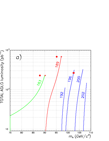
Solving eq. (28) for the existing LEP data with 183 GeV GeV (Table 1) results in a predicted combined exclusion of for the SM Higgs boson (see Figure 17a).
| (GeV) | 182.7 | 188.6 | 191.6 | 195.5 | 199.5 | 201.6 |
|---|---|---|---|---|---|---|
| (pb-1) | 220.0 | 682.7 | 113.9 | 316.4 | 327.8 | 148.1 |
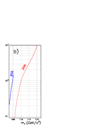
Based on the current LEP operational experience, it is believed that in the year 2000 stable running is possible up to GeV[25]. Figure 17b demonstrates the impact of additional data collected at GeV on the exclusion. For instance, if no evidence of a signal were found in the data, collecting 500 (1000) pb-1 at this centre-of-mass energy would increase the limit to 113.0 (114.1) . Figure 17c shows the degradation in the sensitivity to a Higgs boson signal if the data in the year 2000 were accumulated at GeV instead: in this case the luminosity required to exclude up to would be 840 pb-1.
|
| (GeV) | 204. | 205. | 206. | 208. | ||
|---|---|---|---|---|---|---|
| 1) (pb-1) | - | - | 100. | - | 110.0 | 0.6 – 2.1 |
| 2) (pb-1) | - | - | 500. | - | 113.0 | 0.5 – 2.4 |
| 3) (pb-1) | - | - | 1000. | - | 114.1 | 0.5 – 2.5 |
| 4) (pb-1) | - | 120. | - | - | 110.0 | 0.6 – 2.1 |
| 5) (pb-1) | - | 840. | - | - | 113.0 | 0.5 – 2.4 |
| 6) (pb-1) | 100. | 100. | 400. | - | 113.1 | 0.5 – 2.4 |
| 7) (pb-1) | 150. | 300. | 300. | - | 113.3 | 0.5 – 2.4 |
| 8) (pb-1) | 150. | 300. | 300. | 280. | 115.0 | 0.5 – 2.6 |
In Table 2 the expected SM Higgs boson limit is shown for several possible LEP running scenarios in the year 2000. Taking into account that the experimental MSSM exclusion in the range is (i) essentially independent of and (ii) equal in value to the SM exclusion (see e.g. [24, 26]), can be converted into an excluded range in the benchmark scenario described in Section 9.2. This is done by intersecting the experimental exclusion and the solid curve in Figure 16. Using the LEP data taken until the end of 1999 (for which ) one can already expect to exclude within the MSSM for GeV and TeV. Note that in determining the excluded regions in Table 2 the theoretical uncertainty from unknown higher-order corrections has been neglected. As can be seen from Table 2, several plausible scenarios for adding new data at higher energies can extend the exclusion to ().
9.4 The upper limit on in the M-SUGRA scenario
The M-SUGRA scenario is described by four independent parameters and a sign, namely the common squark mass , the common gaugino mass , the common trilinear coupling , and the sign of . The universal parameters are fixed at the GUT scale, where we assumed unification of the gauge couplings. Then they are run down to the electroweak scale with the help of renormalisation group equations [27, 28, 29, 30, 31, 32, 15, 4]. The condition of REWSB puts an upper bound on of about 5 TeV (depending on the values of the other four parameters).
In order to obtain a precise prediction for within the M-SUGRA scenario, we employ the complete two-loop RG running with appropriate thresholds (both logarithmic and finite for the gauge couplings and using the so called -function approximation for the masses [15]) including full one-loop minimisation conditions for the effective potential, in order to extract all the parameters of the M-SUGRA scenario at the EW scale. This method has been combined with the presently most precise result of based on a Feynman-diagrammatic calculation [8, 9]. This has been carried out by combining the codes of two programs namely, SUITY [33] and FeynHiggs [19].
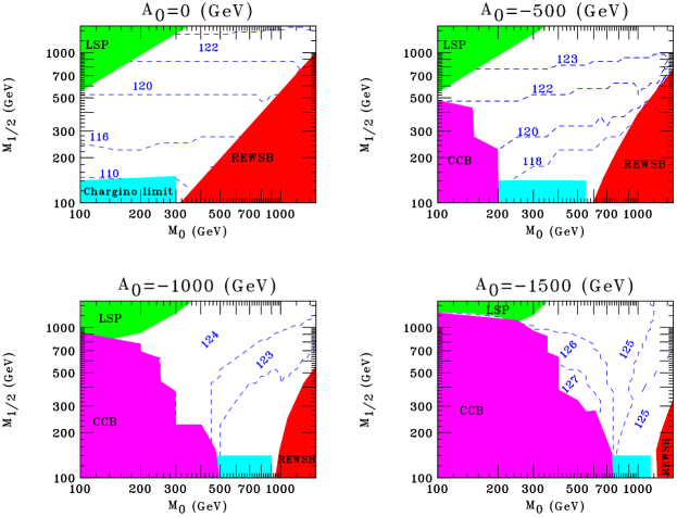
In order to investigate the upper limit on the Higgs boson mass in the M-SUGRA scenario, we keep fixed at a large value, . Concerning the sign of the Higgs mixing parameter, , we find larger values (compatible with the constraints discussed below) for negative (in the convention of eq. (26)). In the following we analysed the upper limit on as a function of the other M-SUGRA parameters, , and . Our results are displayed in Fig. 18 for four values of : . We show contour lines of in the -plane. The numbers inside the plots indicate the lightest Higgs boson mass in the respective area within . The upper bound on the lightest -even Higgs boson mass is found to be at most 127 GeV. This upper limit is reached for , and . Concerning the analysis the following should be noted:
-
•
We have chosen the current experimental central value for the top quark mass, GeV. As mentioned above, increasing by 1 GeV results in an increase of of approximately .
-
•
The M-SUGRA parameters are taken to be real, no SUSY -violating phases are assumed.
-
•
We have chosen negative values for the trilinear coupling, because turns out to be increased by going from positive to negative values of . is restricted from above by the condition that no negative squares of squark masses and no charge or colour breaking minima appear.
-
•
The regions in the -plane that are excluded for the following reasons are also indicated:
-
–
REWSB: parameter sets that do not fulfil the REWSB condition.
-
–
CCB: regions where charge or colour breaking minima occur or negative squared squark masses are obtained at the EW scale.
-
–
LSP: sets where the lightest neutralino is not the LSP. Mostly there the lightest scalar tau becomes the LSP.
-
–
Chargino limit: parameter sets which correspond to a chargino mass that is already excluded by direct searches.
-
–
- •
9.5 Conclusions
We have analysed the upper bound on within the MSSM. Using the Feynman-diagrammatic result for , which contains new genuine two-loop corrections, leads to an increase of of up to compared to the previous result obtained by renormalisation group methods. We have furthermore investigated the MSSM parameters for which the maximal values are obtained and have compared the scenario with the previous benchmark scenario. For GeV and TeV we find GeV as upper bound in the MSSM. In case that no evidence of a Higgs signal is found before the end of running in 2000, experimental searches for the Higgs boson at LEP can ultimately be reasonably expected to exclude . In the context of the benchmark scenario (with GeV, TeV) this rules out the interval at the 95% confidence level within the MSSM. Within the M-SUGRA scenario, the upper bound on is found to be for . This upper limit is reached for the M-SUGRA parameters , and . The upper bound within the M-SUGRA scenario is lower by 2 and 4 GeV than the bound obtained in the general MSSM for and , respectively.
References
References
- [1] H. Haber and R. Hempfling, Phys. Rev. Lett. 66 (1991) 1815; J. Ellis, G. Ridolfi and F. Zwirner, Phys. Lett. B 257 (1991) 83; Phys. Lett. B 262 (1991) 477.
- [2] P. Chankowski, S. Pokorski and J. Rosiek, Nucl. Phys. B 423 (1994) 437.
- [3] A. Dabelstein, Nucl. Phys. B 456 (1995) 25, hep-ph/9503443; Z. Phys. C 67 (1995) 495, hep-ph/9409375.
- [4] J. Bagger, K. Matchev, D. Pierce and R. Zhang, Nucl. Phys. B 491 (1997) 3, hep-ph/9606211.
- [5] M. Carena, J. Espinosa, M. Quirós and C. Wagner, Phys. Lett. B 355 (1995) 209, hep-ph/9504316; M. Carena, M. Quirós and C. Wagner, Nucl. Phys. B 461 (1996) 407, hep-ph/9508343.
- [6] H. Haber, R. Hempfling and A. Hoang, Z. Phys. C 75 (1997) 539, hep-ph/9609331.
- [7] R. Hempfling and A. Hoang, Phys. Lett. B 331 (1994) 99, hep-ph/9401219; R.-J. Zhang, Phys. Lett. B 447 (1999) 89, hep-ph/9808299.
- [8] S. Heinemeyer, W. Hollik and G. Weiglein, Phys. Rev. D 58 (1998) 091701, hep-ph/9803277; Phys. Lett. B 440 (1998) 296, hep-ph/9807423.
- [9] S. Heinemeyer, W. Hollik and G. Weiglein, Eur. Phys. Jour. C 9 (1999) 343, hep-ph/9812472.
- [10] A. Blondel, ALEPH Collaboration, talk given at the LEPC meeting, November 9, 1999.
- [11] J. Marco, DELPHI Collaboration, talk given at the LEPC meeting, November 9, 1999.
- [12] G. Rahal-Callot, L3 Collaboration, talk given at the LEPC meeting, November 9, 1999.
- [13] P. Ward, OPAL Collaboration, talk given at the LEPC meeting, November 9, 1999.
-
[14]
L.E. Ibañez and G.G. Ross, Phys. Lett.
110 (1982) 215;
K. Inoue, A. Kakuto, H. Komatsu and S. Takeshita, Progr. Theor. Phys. 68 (1982) 927; ibidem, 71 (1984) 96;
J. Ellis, D.V. Nanopoulos and K. Tamvakis, Phys. Lett. B121 (1983) 123;
L.E. Ibañez , Nucl. Phys. B218 (1983) 514;
L. Alvarez-Gaumé, J. Polchinski and M. Wise, Nucl. Phys. B221 (1983) 495;
J. Ellis, J.S. Hagelin, D.V. Nanopoulos and K. Tamvakis, Phys. Lett. B125 (1983) 275;
L. Alvarez-Gaumé, M. Claudson and M. Wise, Nucl. Phys. B207 (1982) 96. - [15] A. Dedes, A.B. Lahanas and K. Tamvakis, Phys. Rev. D53, 3793 (1996) hep-ph/9504239;
- [16] The LEP working group for Higgs boson searches, CERN-EP/99-060.
- [17] S. Heinemeyer, W. Hollik and G. Weiglein, DESY 99-120, hep-ph/9909540.
- [18] M. Carena, S. Heinemeyer, C. Wagner and G. Weiglein, hep-ph/9912223.
- [19] S. Heinemeyer, W. Hollik and G. Weiglein, Comp. Phys. Comm. 124 (2000) 76.
- [20] M. Carena, H. Haber, S. Heinemeyer, W. Hollik, C. Wagner and G. Weiglein, hep-ph/0001002.
- [21] S. Heinemeyer, W. Hollik and G. Weiglein, Phys. Lett. B 455 (1999) 179, hep-ph/9903404; hep-ph/9910283.
- [22] P. Janot, How should we organize the Higgs safari?, published in the Proceedings of the 9th Chamonix SPS & LEP Performance Workshop, January 1999 (J. Poole, Ed.); CERN-SL-99-007-DI.
- [23] The LEP working group for Higgs boson searches, CERN-EP/98-046.
- [24] The LEP working group for Higgs boson searches, paper #6_49, submitted to the the International Europhysics Conference on High Energy Physics, July 1999, Tampere, Finland; ALEPH 99-081, DELPHI 99-142, L3 note 2442, OPAL TN-614.
- [25] A. Butterworth, talk given at the LEPC meeting, November 9, 1999.
- [26] P. McNamara, Combined LEP Higgs search results up to 196 GeV, talk given at the LEPC meeting, September 7, 1999.
- [27] G.G. Ross and R.G. Roberts, Nucl. Phys. B377, 571 (1992).
- [28] P. Nath and R. Arnowitt, Phys. Lett. B287, 89 (1992).
- [29] A. Faraggi and B. Grinstein, Nucl. Phys. B422, 3 (1994).
- [30] D.J. Castano, E.J. Piard and P. Ramond, Phys. Rev. D49, 4882 (1994) hep-ph/9308335.
- [31] V. Barger, M.S. Berger and P. Ohmann, Phys. Rev. D49, 4908 (1994) hep-ph/9311269.
- [32] G.L. Kane, C. Kolda, L. Roszkowski and J.D. Wells, Phys. Rev. D49, 6173 (1994) hep-ph/9312272.
- [33] A. Dedes, A. B. Lahanas, V. Spanos and K. Tamvakis, “SUITY: A program for the minimal SUpergravITY spectrum”, in preparation.
- [34] K. Matchev and D. Pierce, Phys. Lett. B445, 331 (1999).
-
[35]
W. de Boer, H.J. Grimm, A.V. Gladyshev, D.I. Kazakov,
Phys. Lett. B438, 281 (1998);
W. de Boer, talk given at the ECFA/DESY Linear Collider Workshop, Obernai, October 1999.
10 An Update of the program HDECAY
A Djouadi, J Kalinowski and M Spira
The search strategies for Higgs bosons at LEP, Tevatron, LHC and future linear colliders (LC) exploit various Higgs boson decay channels. The strategies depend not only on the experimental setup (hadron versus lepton colliders) but also on the theoretical scenarios: the Standard Model (SM) or some of its extensions such as the Minimal Supersymmetric Standard Model (MSSM). It is of vital importance to have reliable predictions for the branching ratios of the Higgs boson decays for these theoretical models.
The current version of the program HDECAY [1] can be used to calculate Higgs boson partial decay widths and branching ratios within the SM and the MSSM and includes:
– All decay channels that are kinematically allowed and which have
branching ratios larger than , y compris the loop
mediated, the three body decay modes and in the MSSM the cascade and
the supersymmetric decay channels [2].
– All relevant higher-order QCD corrections to the decays into quark
pairs and to the loop mediated decays into gluons are incorporated in
a complete form [3]; the small leading electroweak corrections
are also included.
– Double off–shell decays of the CP–even Higgs bosons into massive
gauge bosons which then decay into four massless fermions, and all
important below–threshold three–body decays [4].
– In the MSSM, the complete radiative corrections in the effective
potential approach with full mixing in the stop/sbottom sectors; it
uses the renormalisation group improved values of the Higgs masses and
couplings and the relevant next–to–leading–order corrections are
implemented [5].
– In the MSSM, all the decays into SUSY particles (neutralinos,
charginos, sleptons and squarks including mixing in the stop, sbottom
and stau sectors) when they are kinematically allowed [6]. The
SUSY particles are also included in the loop mediated
and decay channels.
The source code of the program, written in FORTRAN, has been tested on computers running under different operating systems. The program provides a very flexible and convenient usage, fitting to all options of phenomenological relevance. The basic input parameters, fermion and gauge boson masses and their total widths, coupling constants and, in the MSSM, soft SUSY-breaking parameters can be chosen from an input file. In this file several flags allow switching on/off or changing some options [e.g. choosing a particular Higgs boson, including/excluding the multi-body or SUSY decays, or including/excluding specific higher-order QCD corrections].
Since the release of the original version of the program several bugs have been fixed and a number of improvements and new theoretical calculations have been implemented. The following points have recently been done:
– Link to the FeynHiggsFast routine for Higgs masses and couplings
[7].
– Link to the SUSPECT routine for RG evolution of SUGRA parameters
[8].
– Implementation of Higgs boson decays to gravitino + gaugino [9].
– Inclusion of gluino loops in Higgs decays to [10].
– Inclusion of QCD corrections in Higgs decays to squarks [11].
– Determination and inclusion of the RG improved two-loop contributions to
the MSSM Higgs self-interactions.
The logbook of all modifications and the most recent version of the program can be found on the web page http://www.desy.de/spira/prog.
References
References
- [1] A. Djouadi, J. Kalinowski and M. Spira, Comput. Phys. Commun. 108 (1998) 56.
- [2] M. Spira, Fortschr. Phys. 46 (1998) 203.
- [3] A. Djouadi, M. Spira and P.M. Zerwas, Z. Phys. C70 (1996) 427.
- [4] A. Djouadi, J. Kalinowski and P.M. Zerwas, Z. Phys. C70 (1996) 435.
- [5] M. Carena, M. Quiros and C.E.M. Wagner, Nucl. Phys. B461 (1996) 407; H.E. Haber, R. Hempfling and A.H. Hoang, Z. Phys. C75 (1997) 539; S. Heinemeyer, W. Hollik and G. Weiglein, Phys. Rev. D58 (1998) 091701.
- [6] A. Djouadi, J. Kalinowski and P.M. Zerwas, Z. Phys. C57 (1993) 569; A. Djouadi, P. Janot, J. Kalinowski and P.M. Zerwas, Phys. Lett. B376 (1996) 220; A. Djouadi, J. Kalinowski, P. Ohmann and P.M. Zerwas, Z. Phys. C74 (1997) 93.
- [7] S. Heinemeyer, W. Hollik and G. Weiglein, Comp. Phys. Comm. 124 (2000) 76.
- [8] A. Djouadi, J.L. Kneur and G. Moultaka, in hep-ph/9901246.
- [9] A. Djouadi and M. Drees, Phys. Lett. B407 (1997) 243.
- [10] A. Dabelstein, Nucl. Phys. B456 (1995) 25; R.A. Jiménez and J. Solà, Phys. Lett. B389 (1996) 53; J.A. Coarasa, R.A. Jiménez and J. Solà, Phys. Lett. B389 (1996) 312.
- [11] A. Bartl, H. Eberl, K. Hidaka, T. Kon, W. Majerotto and Y. Yamada, Phys. Lett. B402 (1997) 303; A. Arhrib, A. Djouadi, W. Hollik and C. Jünger, Phys. Rev. D57 (1998) 5860.