Neutrino oscillations with three flavors in matter: Applications to neutrinos traversing the Earth

Abstract

Analytic formulas are presented for three flavor neutrino oscillations in matter in the plane wave approximation. We calculate in particular the time evolution operator in both mass and flavor bases. We also find the transition probabilities expressed as functions of the vacuum mass squared differences, the vacuum mixing angles, and the matter density parameter. The application of this to neutrino oscillations for both atmospheric and long baseline neutrinos in a mantle-core-mantle step function model of the Earth’s matter density profile is discussed.

PACS: 14.60.Pq, 14.60.Lm, 13.15.+g, 96.40.Tv

,

1 Introduction

As an accumulating amount of data on neutrino oscillations is becoming accessible, it is of interest to study three flavor neutrino oscillations. Here we would like to give analytic expressions for the neutrino oscillation probabilities in presence of matter expressed in the mixing matrix elements and the neutrino energies or masses, i.e., incorporating the so called Mikheyev–Smirnov–Wolfenstein (MSW) effect [1, 2]. These probability formulas are of interest for the solar neutrino problem, the atmospheric neutrino problem, and the long baseline (LBL) neutrino experiments. We here apply the formalism to neutrinos traversing the Earth in a mantle-core-mantle step function model of the Earth’s matter density profile.

We will assume that $CP$ nonconservation is negligible at the present level of experimental accuracy [3]. Thus, the mixing matrix for the neutrinos is real.

Previous work on models for three flavor neutrino oscillations in matter includes works of Barger et al. [4], Kim and Sze [5], and Zaglauer and Schwarzer [6]. Our method is different from all these approaches and their parameterizations also differ slightly from ours. In particular, we calculate the time evolution operator and do not use the auxiliary matter mixing angles.

Approximate solutions for three flavor neutrino oscillations in matter have been presented by Kuo and Pantaleone [7] and Joshipura and Murthy [8]. Approximate treatments have also been done by Toshev and Petcov [9]. D’Olivo and Oteo have made contributions by using an approximative Magnus expansion for the time evolution operator [10]. Extensive numerical investigations for matter enhanced three flavor oscillations have been made by Fogli et al. [11]. Studies of neutrino oscillations in the Earth has been performed by several authors [12, 13, 14, 15, 16, 17, 18].

2 The evolution operator

Let the flavor state basis and mass eigenstate basis be given by ${\cal H}_{f}\equiv\{|\nu_{\alpha}\rangle\}_{\alpha=e,\mu,\tau}$ and ${\cal H}_{m}\equiv\{|\nu_{a}\rangle\}_{a=1}^{3}$, respectively. Then the flavor states $|\nu_{\alpha}\rangle\in{\cal H}_{f}$ can be obtained as superpositions of the mass eigenstates $|\nu_{a}\rangle\in{\cal H}_{m}$, or vice versa. The bases ${\cal H}_{f}$ and ${\cal H}_{m}$ are of course just two different representations of the same Hilbert space ${\cal H}$.

In the present analysis, we will use the plane wave approximation to describe neutrino oscillations. In this approximation, a neutrino flavor state $|\nu_{\alpha}\rangle$ is a linear combination of neutrino mass eigenstates $|\nu_{a}\rangle$ such that [19]

$$|\nu_{\alpha}\rangle=\sum_{a=1}^{3}U^{\ast}_{\alpha a}|\nu_{a}\rangle,$$ (1)

where $\alpha=e,\mu,\tau$. In what follows, we will use the short-hand notations $|\alpha\rangle\equiv|\nu_{\alpha}\rangle$ and $|a\rangle\equiv|\nu_{a}\rangle$ for the flavor states and the mass eigenstates, respectively.

For the components of a state $\psi$ in the flavor state basis and mass eigenstate basis, respectively, they are related to each other by

$$\psi_{f}=U\psi_{m},$$ (2)

where

$$\psi_{f}=\left(\psi_{\alpha}\right)=\left(\begin{array}[]{c}\psi_{e}\\ \psi_{\mu}\\ \psi_{\tau}\end{array}\right)\in{\cal H}_{f}\quad\mbox{and}\quad\psi_{m}=\left(\psi_{a}\right)=\left(\begin{array}[]{c}\psi_{1}\\ \psi_{2}\\ \psi_{3}\end{array}\right)\in{\cal H}_{m}.$$

A convenient parameterization for $U=U(\theta_{1},\theta_{2},\theta_{3})$ is given by [20]

$$U=\left(\begin{array}[]{ccc}C_{2}C_{3}&S_{3}C_{2}&S_{2}\\ -S_{3}C_{1}-S_{1}S_{2}C_{3}&C_{1}C_{3}-S_{1}S_{2}S_{3}&S_{1}C_{2}\\ S_{1}S_{3}-S_{2}C_{1}C_{3}&-S_{1}C_{3}-S_{2}S_{3}C_{1}&C_{1}C_{2}\end{array}\right),$$ (3)

where $S_{i}\equiv\sin\theta_{i}$ and $C_{i}\equiv\cos\theta_{i}$ for $i=1,2,3$. This is the standard representation of the mixing matrix. The quantities $\theta_{i}$, where $i=1,2,3$, are the vacuum mixing angles. Since we have put the $CP$ phase equal to zero in the mixing matrix, this means that $U^{\ast}_{\alpha a}=U_{\alpha a}$ for $\alpha=e,\mu,\tau$ and $a=1,2,3$.

In the mass eigenstate basis, the Hamiltonian ${\mathscr{H}}$ for the propagation of the neutrinos in vacuum is diagonal and given by

$$H_{m}=\left(\begin{array}[]{ccc}E_{1}&0&0\\ 0&E_{2}&0\\ 0&0&E_{3}\end{array}\right),$$ (4)

where $E_{a}=\sqrt{m_{a}^{2}+{\bf p}^{2}}$, $a=1,2,3$, are the energies of the neutrino mass eigenstates $|a\rangle$, $a=1,2,3$ with masses $m_{a}$, $a=1,2,3$. We will assume ${\bf p}$ to be the same for all mass eigenstates.

When neutrinos propagate in matter, there is an additional term coming from the presence of electrons in matter [2]. This term is diagonal in the flavor state basis and is given by

$$V_{f}=\left(\begin{array}[]{ccc}A&0&0\\ 0&0&0\\ 0&0&0\end{array}\right),$$ (5)

where

$$A=\pm\sqrt{2}G_{F}N_{e}\simeq\pm\frac{1}{\sqrt{2}}G_{F}\frac{1}{m_{N}}\rho$$

is the matter density parameter. Here $G_{F}$ is the Fermi weak coupling constant, $N_{e}$ is the electron density, $m_{N}$ is the nucleon mass, and $\rho$ is the matter density. The sign depends on whether we deal with neutrinos ($+$) or antineutrinos ($-$). We will assume that the electron density $N_{e}$ (or the matter density $\rho$) is constant throughout the matter in which the neutrinos are propagating. In the mass basis, this piece of the Hamiltonian is $V_{m}=U^{-1}V_{f}U$, where again $U$ is the mixing matrix.

The unitary transformation that leads from the initial state $\psi_{f}(0)$ in flavor basis at time $t=0$ of production of the neutrino, to the state of the same neutrino $\psi_{f}(t)$ at the detector at time $t$ is given by the operator $U_{f}(t)\equiv U_{f}(t,0)$, where $U_{f}(t_{2},t_{1})$ is the time evolution operator from time $t_{1}$ to time $t_{2}$ in flavor basis. This operator can be formally written as $U_{f}(t)=e^{-iH_{f}t}$. When the neutrinos are propagating through vacuum, the Hamiltonian in flavor basis is $H_{f}=UH_{m}U^{-1}$. In this case, the exponentiation of $H_{f}$ can be performed easily: $U_{f}(t)=e^{-iH_{f}t}=Ue^{-iH_{m}t}U^{-1}$, and the result can be expressed in closed form. In the case when the neutrinos propagate through matter, the Hamiltonian is not diagonal in either the mass eigenstate basis or the flavor state basis, and we have to calculate the evolution operator $U_{f}(t)$ or $U_{f}(L)\equiv e^{-i{\mathscr{H}}_{f}L}=Ue^{-i{\mathscr{H}}_{m}L}U^{-1}$ if we set $t=L$.

To do so it is convenient to introduce the traceless matrix $T$ defined by $T\equiv{\mathscr{H}}_{m}-({\rm tr\,}{\mathscr{H}}_{m})I/3$. The trace of the Hamiltonian in the mass basis ${\mathscr{H}}_{m}\equiv H_{m}+U^{-1}V_{f}U$ is ${\rm tr\,}{\mathscr{H}}_{m}=E_{1}+E_{2}+E_{3}+A$, and the matrix $T$ can then be written as

$$T = (T_{ab})$$ (9)

$$= \left(\begin{array}[]{ccc}AU_{e1}^{2}-\tfrac{1}{3}A+\tfrac{1}{3}\left(E_{12}+E_{13}\right)&AU_{e1}U_{e2}&AU_{e1}U_{e3}\\ AU_{e1}U_{e2}&AU_{e2}^{2}-\tfrac{1}{3}A+\tfrac{1}{3}\left(E_{21}+E_{23}\right)&AU_{e2}U_{e3}\\ AU_{e1}U_{e3}&AU_{e2}U_{e3}&AU_{e3}^{2}-\tfrac{1}{3}A+\tfrac{1}{3}\left(E_{31}+E_{32}\right)\end{array}\right),$$

where $E_{ab}\equiv E_{a}-E_{b}$. Of the six quantities $E_{ab}$, where $a,b=1,2,3$ and $a\neq b$, only two are linearly independent, since the $E_{ab}$’s fulfill the relations $E_{ba}=-E_{ab}$ and $E_{12}+E_{23}+E_{31}=0$. Using Eq. (LABEL:eq:T), the evolution operator in the mass basis can be written as

$$U_{m}(L)\equiv e^{-i{\mathscr{H}}_{m}L}=\phi e^{-iLT},$$ (11)

where $\phi\equiv e^{-iL{\rm tr\,}{\mathscr{H}}_{m}/3}$.

The flavor states can be expressed either as linear combinations of the vacuum mass eigenstates ($A=0$) in the basis ${\cal H}_{m}$ as in Eq. (2) or the matter mass eigenstates ($A\neq 0$) in the basis ${\cal H}_{M}$. In the latter case, the corresponding components are related to each other as

$$\psi_{f}=U^{M}\psi_{M},$$ (12)

where $U^{M}=U^{M}(\theta_{1}^{M},\theta_{2}^{M},\theta_{3}^{M})$ is the unitary mixing matrix for matter and $\theta^{M}_{i}$, $i=1,2,3$, are the (auxiliary) matter mixing angles.

Combining these expressions for the flavor state components, one obtains the following relation between the two different sets of mass eigenstate components

$$\psi_{M}=R\psi_{m},$$ (13)

where

$$R\equiv(U^{M})^{-1}U.$$

The matrix $R$ is, of course, a unitary matrix (even orthogonal, since $U$ and $U^{M}$ are real). This means that the matter mixing matrix can be expressed in the vacuum mixing matrix as

$$U^{M}(\theta_{1}^{M},\theta_{2}^{M},\theta_{3}^{M})=U(\theta_{1},\theta_{2},\theta_{3})R^{-1}.$$ (14)

The relations between the different bases are depicted in the following diagram:

From this diagram one readily obtains

$${\mathscr{H}}_{M}\equiv R{\mathscr{H}}_{m}R^{-1}\quad\mbox{or}\quad{\mathscr{H}}_{M}\equiv RTR^{-1}+\tfrac{1}{3}({\rm tr\,}{\mathscr{H}}_{m})I,$$

where ${\mathscr{H}}_{M}$ is the Hamiltonian in matter, which is diagonal in the basis ${\cal H}_{M}$.

Due to the invariance of the trace, we have

$$T_{M}\equiv{\mathscr{H}}_{M}-\tfrac{1}{3}({\rm tr\,}{\mathscr{H}}_{M})I=RTR^{-1}.$$ (15)

and $T_{M}$ is a diagonal matrix with elements $\lambda_{a}$, $a=1,2,3$, the eigenvalues of $T$. This implies that

$$e^{-iLT_{M}}=Re^{-iLT}R^{-1}.$$ (16)

Now, Cayley–Hamilton’s theorem implies that, since $T$ is a $3\times 3$ matrix, the infinite series defining $e^{-iLT}$ can be written as a second order polynomial in $T$ [21]:

$$e^{-iLT}=a_{0}I-iLTa_{1}-L^{2}T^{2}a_{2},$$ (17)

where $a_{0}$, $a_{1}$, and $a_{2}$ are coefficients to be determined. Inserting Eq. (17) into Eq. (16) and using Eq. (15) gives a linear system of three equations that will determine the coefficients $a_{0}$, $a_{1}$, and $a_{2}$:

$$\left\{\begin{array}[]{l}e^{-iL\lambda_{1}}=a_{0}-iL\lambda_{1}a_{1}-L^{2}\lambda_{1}^{2}a_{2}\\ e^{-iL\lambda_{2}}=a_{0}-iL\lambda_{2}a_{1}-L^{2}\lambda_{2}^{2}a_{2}\\ e^{-iL\lambda_{3}}=a_{0}-iL\lambda_{3}a_{1}-L^{2}\lambda_{3}^{2}a_{2}\end{array}\right.,$$ (18)

where $\lambda_{a}$, $a=1,2,3$, are the diagonal elements of $T_{M}$, or, equivalently, the eigenvalues of $T$, i.e., the solutions to the characteristic equation

$$\lambda^{3}+c_{2}\lambda^{2}+c_{1}\lambda+c_{0}=0$$ (19)

with

$$c_{2} = -{\rm tr\,}T=0,$$ (20)

$$c_{1} = \det T\,{\rm tr\,}T^{-1},$$ (21)

$$c_{0} = -\det T.$$ (22)

The coefficients $c_{0}$, $c_{1}$, and $c_{2}$ are all real and the eigenvalues $\lambda_{a}$, $a=1,2,3$, can be expressed in closed form in terms of these [21].

When the system of equations (18) is solved for the $a_{i}$’s, we obtain

$$e^{-iLT}=\sum_{a=1}^{3}e^{-iL\lambda_{a}}\frac{1}{3\lambda_{a}^{2}+c_{1}}\left[(\lambda_{a}^{2}+c_{1})I+\lambda_{a}T+T^{2}\right].$$ (23)

From Eqs. (11) and (23) we then obtain

$$U_{m}(L)=e^{-i{\mathscr{H}}_{m}L}=\phi e^{-iLT}=\phi\sum_{a=1}^{3}e^{-iL\lambda_{a}}\frac{1}{3\lambda_{a}^{2}+c_{1}}\left[(\lambda_{a}^{2}+c_{1})I+\lambda_{a}T+T^{2}\right].$$ (24)

The evolution operator for the neutrinos in flavor basis is thus given by

$$U_{f}(L)=e^{-i{\mathscr{H}}_{f}L}=Ue^{-i{\mathscr{H}}_{m}L}U^{-1}=\phi\sum_{a=1}^{3}e^{-iL\lambda_{a}}\frac{1}{3\lambda_{a}^{2}+c_{1}}\left[(\lambda_{a}^{2}+c_{1})I+\lambda_{a}\tilde{T}+\tilde{T}^{2}\right],$$ (25)

where $\tilde{T}\equiv UTU^{-1}$. Formula (25) is the final expression for the evolution operator. It expresses the time (or $L$) evolution directly in term of the mass squared differences and the vacuum mixing angles without introducing the auxiliary matter mixing angles.

3 Transition probabilities

The probability amplitude is defined as

$$A_{\alpha\beta}\equiv\langle\beta|U_{f}(L)|\alpha\rangle,\quad\alpha,\beta=e,\mu,\tau.$$ (26)

Inserting Eq. (25) into Eq. (26) gives

$$A_{\alpha\beta}=\phi\sum_{a=1}^{3}e^{-iL\lambda_{a}}\frac{(\lambda_{a}^{2}+c_{1})\delta_{\alpha\beta}+\lambda_{a}\tilde{T}_{\alpha\beta}+(\tilde{T}^{2})_{\alpha\beta}}{3\lambda_{a}^{2}+c_{1}},$$ (27)

where $\delta_{\alpha\beta}$ is Kronecker’s delta. Note that $\tilde{T}_{\alpha\beta}=\tilde{T}_{\beta\alpha}$ and $(\tilde{T}^{2})_{\alpha\beta}=(\tilde{T}^{2})_{\beta\alpha}$.

Inserting $L=0$ into Eq. (25) yields

$$\delta_{\alpha\beta}=\sum_{a=1}^{3}\frac{(\lambda_{a}^{2}+c_{1})\delta_{\alpha\beta}+\lambda_{a}\tilde{T}_{\alpha\beta}+(\tilde{T}^{2})_{\alpha\beta}}{3\lambda_{a}^{2}+c_{1}}.$$ (28)

Hence, the transition probabilities in matter are

$$P_{\alpha\beta}=|A_{\alpha\beta}|^{2} = \delta_{\alpha\beta}-4\;\underset{a<b}{\sum_{a=1}^{3}\sum_{b=1}^{3}}\frac{(\lambda_{a}^{2}+c_{1})\delta_{\alpha\beta}+\lambda_{a}\tilde{T}_{\alpha\beta}+(\tilde{T}^{2})_{\alpha\beta}}{3\lambda_{a}^{2}+c_{1}}$$

$$\times \frac{(\lambda_{b}^{2}+c_{1})\delta_{\alpha\beta}+\lambda_{b}\tilde{T}_{\alpha\beta}+(\tilde{T}^{2})_{\alpha\beta}}{3\lambda_{b}^{2}+c_{1}}\sin^{2}\tilde{x}_{ab},\quad\alpha,\beta=e,\mu,\tau,$$

where $\tilde{x}_{ab}\equiv(\lambda_{a}-\lambda_{b})L/2$.

From unitarity, there are only three independent transition probabilities, since the other three can be obtained from them, i.e., from the equations

$$P_{ee}+P_{e\mu}+P_{e\tau}=1,$$ (30)

$$P_{\mu e}+P_{\mu\mu}+P_{\mu\tau}=1,$$ (31)

$$P_{\tau e}+P_{\tau\mu}+P_{\tau\tau}=1.$$ (32)

Note that $P_{e\mu}=P_{\mu e}$, $P_{e\tau}=P_{\tau e}$, and $P_{\mu\tau}=P_{\tau\mu}$. If we choose $P_{e\mu}$, $P_{e\tau}$, and $P_{\mu\tau}$ as the three independent ones, we thus have for $\alpha\neq\beta$

$$P_{\alpha\beta}=-4\;\underset{a<b}{\sum_{a=1}^{3}\sum_{b=1}^{3}}\frac{\lambda_{a}\tilde{T}_{\alpha\beta}+(\tilde{T}^{2})_{\alpha\beta}}{3\lambda_{a}^{2}+c_{1}}\frac{\lambda_{b}\tilde{T}_{\alpha\beta}+(\tilde{T}^{2})_{\alpha\beta}}{3\lambda_{b}^{2}+c_{1}}\sin^{2}\tilde{x}_{ab}.$$ (33)

4 Applications and discussion

The main results of our analysis are given by the time evolution operator for the neutrinos when passing through matter with constant matter density in Eq. (25) and the expression for the transition probabilities in Eqs. (LABEL:eq:Pab_2) and (33), expressed as finite sums of elementary functions in the elements of $\tilde{T}$.

In our treatment the auxiliary mixing angles in matter, $\theta^{M}_{i}$, play no independent role and are not really needed.

When the neutrinos travel through a series of matter densities with matter density parameters $A_{1},\ldots,A_{n}$ and thicknesses $L_{1},\ldots,L_{n}$, the total evolution operator is simply given by

$$U_{f}(L)=\prod_{i=1}^{n}U_{f}(L_{i})=U_{f}(L_{n})\ldots U_{f}(L_{1}),$$ (34)

where $L\equiv\sum_{i=1}^{n}L_{i}$ and $U_{f}(L_{i})$ is calculated for $A=A_{i}$. Equation (34) gives a simple and fast algorithm to obtain the total evolution operator instead of using numerical integration.

As an application to show the usefulness of our derived formulas, we have calculated the transition probabilities $P_{\alpha\beta}$ for neutrino oscillations in a mantle-core-mantle step function model simulating the Earth’s matter density profile. Let $R\simeq 6371$ km be the radius of the Earth and $r\simeq 3486$ km be the radius of the core. The thickness of the mantle is then $R-r\simeq 2885$ km, with matter density parameter $A_{1}\simeq 1.70\cdot 10^{-13}$ eV ($\rho_{1}\simeq 4.5$ ${\rm g/cm^{3}}$), whereas the matter density parameter of the core is $A_{2}\simeq 4.35\cdot 10^{-13}$ eV ($\rho_{2}\simeq 11.5$ ${\rm g/cm^{3}}$).

Neutrinos traversing the Earth towards a detector close to the surface of the Earth, pass through the matter densities $A_{1},A_{2},A_{1}$ of thicknesses $L_{1},L_{2},L_{1}$ where the distances $L_{i}$, $i=1,2$, are functions of the nadir angle $h$, where $h\equiv 180^{\circ}-\theta_{z}$; $\theta_{z}$ being the zenith angle. As $h$ varies from $0$ to $90^{\circ}$, the cord $L=L(h)$ of the neutrino passage through the Earth becomes shorter and shorter. At an angle larger than $h_{0}=\arcsin(r/R)\simeq 33.17^{\circ}$, the distance $L_{2}=0$, and the neutrinos no longer traverse the core.

For $0\leq h\leq h_{0}$ the distances $L_{1}$ and $L_{2}$ are given by

$$L_{1} = R\left(\cos h-\sqrt{\left(\frac{r}{R}\right)^{2}-\sin^{2}h}\right),$$ (35)

$$L_{2} = 2R\sqrt{\left(\frac{r}{R}\right)^{2}-\sin^{2}h},$$ (36)

$$L = 2L_{1}+L_{2}.$$ (37)

For $h_{0}\leq h\leq 90^{\circ}$:

$$L=2R\cos h.$$ (38)

The mass squared differences ($\Delta M^{2}\equiv\Delta m_{32}^{2}$ and $\Delta m^{2}\equiv\Delta m_{21}^{2}$) and the vacuum mixing angles ($\theta_{1},\theta_{2},\theta_{3}$) used here are chosen to correspond to those obtained from analyses of various neutrino oscillation data. For our illustration we have taken the following parameter values

$$\Delta M^{2}=3.2\cdot 10^{-3}{\rm eV}^{2},\quad\Delta m^{2}=0,\Delta M^{2}/10,\quad\theta_{1}=45^{\circ},\quad\theta_{2}=5^{\circ},\quad\theta_{3}=45^{\circ}.$$

The values of $\Delta M^{2}$ and $\theta_{1}$ are governed by atmospheric neutrino data [22] and the values of $\Delta m^{2}$ and $\theta_{3}$ by solar neutrino data [23]. The value of $\theta_{2}$ is below the CHOOZ upper bound, which is $\sin^{2}2\theta_{2}=0.10$ [24]. These choices are the most optimistic ones for obtaining any effects in LBL experiments from the sub-leading $\Delta m^{2}$ scale [25]. We should mention though, that these data are taken from two flavor model analyses.

The probabilities corresponding to various situations in this scenario are illustrated in Figs. 1 - 4. These figures correspond to the physically measurable quantities. From the figures one can see that there are several resonance phenomena superimposed on each other.

Figures 1 a) - 1 d) show the results for the case of $h=0$, one mass squared difference equal to $3.2\cdot 10^{-3}$ ${\rm eV}^{2}$ [22], and the other one equal to 0. In Fig. 1 a) we have included for comparison the corresponding result of a two flavor model. Figures 1 b) - 1 d) show the probabilities $P_{ee}$, $P_{e\mu}$, and $P_{\mu\tau}$, respectively, in the three flavor model. The other probabilities can be obtained by unitarity from these three using Eqs. (30) - (32). We observe that although the survival probability $P_{ee}$ is the same for both cases, the transition probability $P_{e\mu}$ is only half of that in the two flavor model. In a two flavor model, only one transition probability is needed, since if $P_{ee}$ is given and $P_{\mu e}=P_{e\mu}$, the other two follow from $P_{e\mu}=1-P_{ee}$ and $P_{\mu\mu}=1-P_{e\mu}=P_{ee}$.

In Figs. 2 a) - d) the second mass squared difference is chosen to be $1/10$ of the first one. This affects the disappearance rate for low energies in the three flavor case, as can be seen from Fig. 2 b). It also modifies the appearance rates $P_{e\mu}$ and $P_{\mu\tau}$ in Figs. 2 c) and 2 d), respectively. Figure 2 a) is again the same as Fig. 1 a).

When the small mass squared difference is much smaller than the large mass squared difference, then the two flavor model coincides with the three flavor model. This is not the case when the small mass squared difference is of comparable size to the large mass squared difference. See Figs. 1 a), 1 b), 2 a), and 2 b) for a comparison.

Figure 3 shows a contour plot of $P_{ee}$ as a function of the matter density parameter of the core $A_{\rm core}$ (as it changes from the value of the mantle $A_{1}$ up to its full value $A_{2}$) and the neutrino energy $E_{\nu}$. The dark areas correspond to regions of large conversion probability for the assumed parameter values. When the small mass squared difference decreases, the structure below the main conversion valley goes away. Furthermore, the conversion regions above the main conversion valley are obviously due to the core (either purely to the core or to interference effects between the core and the mantle).

Similarly, Fig. 4 shows a contour plot of $P_{ee}$ as a function of the nadir angle $h$ and the neutrino energy $E_{\nu}$. As in the previous figure, the dark areas correspond to regions of large conversion probability for the assumed parameter values. At $h=h_{0}$, the neutrinos no longer traverse the core, but only the mantle. Again, when the small mass squared difference drops, the oscillations in the bottom of the plot (sub-GeV region) go away and no conversion takes place, i.e., $P_{ee}\simeq 1$ in this region. In the limit when the nadir angle goes to $90^{\circ}$, the survival probability $P_{ee}$ becomes 1, because the traveling path length $L$ of the neutrinos approaches 0.

The results and the applications presented here are relevant to both the atmospheric neutrino experiments (e.g. Super-Kamiokande) and the LBL neutrino experiments. The present treatment assumes that in the results of the atmospheric and LBL experiments, the scattering and absorption of the neutrinos in matter is taken care of in the Monte Carlo programs that are used to analyze the data from these experiments. In a realistic analysis, we should also introduce damping due to uncertainties in the energy $E_{\nu}$ of the neutrinos and their path length $L$.

Examining some of the future LBL neutrino experiments, we find their nadir angles to be $h\simeq 86.7^{\circ}$, $h\simeq 86.7^{\circ}$, and $h\simeq 88.9^{\circ}$ for CERN-NGS ($L=743$ km), MINOS ($L=732$ km), and K2K ($L=252$ km), respectively [25, 26]. See Fig. 4 for how the survival probability $P_{ee}$ depends on the neutrino energy for these fixed nadir angles. Note that for these three experiments the neutrinos only traverse the mantle and not the core.

There are, at the moment, no planned LBL experiments in which the neutrinos also traverse the core. The baseline has in that case to be longer than $L\simeq 10670$ km.

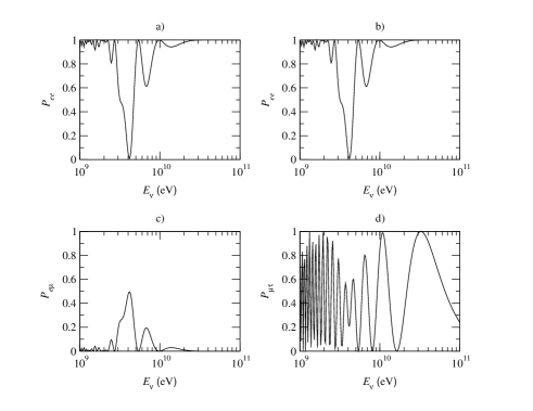
Figure 1: Transition probabilities as functions of the neutrino energy $E_{\nu}$ for the parameter values $h=0$, $\theta_{1}=\theta_{3}=45^{\circ}$ (bimaximal mixing), $\theta_{2}=5^{\circ}$, $\Delta M^{2}=3.2\cdot 10^{-3}$ ${\rm eV}^{2}$, and $\Delta m^{2}=0$. a) $P_{ee}$ (two flavors; parameters values: $\theta=5^{\circ}$ and $\Delta m^{2}=3.2\cdot 10^{-3}$ ${\rm eV^{2}}$), b) $P_{ee}$ (three flavors), c) $P_{e\mu}$ (three flavors), and d) $P_{\mu\tau}$ (three flavors).

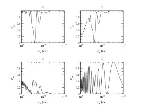
Figure 2: Transition probabilities as functions of the neutrino energy $E_{\nu}$, using the same parameter values as for Fig. 1 except that $\Delta m^{2}=\Delta M^{2}/10$. a) $P_{ee}$ (two flavors; parameters values: $\theta=5^{\circ}$ and $\Delta m^{2}=3.2\cdot 10^{-3}$ ${\rm eV^{2}}$), b) $P_{ee}$ (three flavors), c) $P_{e\mu}$ (three flavors), and d) $P_{\mu\tau}$ (three flavors).

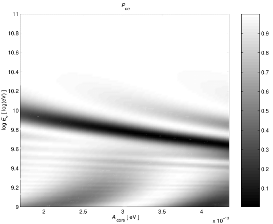
Figure 3: The survival probability $P_{ee}$ as a function of the core matter density parameter $A_{\rm core}\in[A_{1},A_{2}]$ and the neutrino energy $E_{\nu}$, using the same parameter values as for Fig. 2.

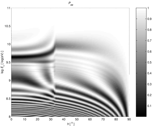
Figure 4: The survival probability $P_{ee}$ as a function of the nadir angle $h$ and the neutrino energy $E_{\nu}$, using the same parameter values as for Fig. 2.

References

- [1] S.P. Mikheyev and A.Yu. Smirnov, Yad. Fiz. 42 (1985) 1441 [Sov. J. Nucl. Phys. 42 (1985) 913]; Nuovo Cimento C 9 (1986) 17.
- [2] L. Wolfenstein, Phys. Rev. D 17 (1978) 2369; 20 (1979) 2634.
- [3] K. Dick, M. Freund, M. Lindner, and A. Romanino, Nucl. Phys. B (to be published), hep-ph/9903308.
- [4] V. Barger, K. Whisnant, S. Pakvasa, and R.J.N. Phillips, Phys. Rev. D 22 (1980) 2718.
- [5] C.W. Kim and W.K. Sze, Phys. Rev. D 35 (1987) 1404.
- [6] H.W. Zaglauer and K.H. Schwarzer, Z. Phys. C 40 (1988) 273.
- [7] T.K. Kuo and J. Pantaleone, Phys. Rev. Lett. 57 (1986) 1805.
- [8] A.S. Joshipura and M.V.N. Murthy, Phys. Rev. D 37 (1988) 1374.
- [9] S. Toshev, Phys. Lett. B 185 (1987) 177; 192 (1987) 478(E); S.T. Petcov and S. Toshev, Phys. Lett. B 187 (1987) 120; S.T. Petcov, Phys. Lett. B 214 (1988) 259.
- [10] J.C. D’Olivo and J.A. Oteo, Phys. Rev. D 54 (1996) 1187.
- [11] G.L. Fogli, E. Lisi, and D. Montanino, Phys. Rev. D 49 (1994) 3626; G.L. Fogli, E. Lisi, and D. Montanino, Phys. Rev. D 54 (1996) 2048, hep-ph/9605273; G.L. Fogli, E. Lisi, D. Montanino, and G. Scioscia, Phys. Rev. D 55 (1997) 4385, hep-ph/9607251; G.L. Fogli, E. Lisi, A. Marrone, and G. Scioscia, Phys. Rev. D 59 (1999) 033001, hep-ph/9808205.
- [12] A. Nicolaidis, Phys. Lett. B 200 (1988) 553.
- [13] P.I. Krastev and S.T. Petcov, Phys. Lett. B 205 (1988) 84.
- [14] C. Giunti, C.W. Kim, and M. Monteno, Nucl. Phys. B 521 (1998) 3, hep-ph/9709439.
- [15] Q.Y. Liu and A.Yu. Smirnov, Nucl. Phys. B 524 (1998) 505, hep-ph/9712493; Q.Y. Liu, S.P. Mikheyev, and A.Yu. Smirnov, Phys. Lett. B 440 (1998) 319, hep-ph/9803415; P. Lipari and M. Lusignoli, Phys. Rev. D 58 (1998) 073005, hep-ph/9803440; E.Kh. Akhmedov, Nucl. Phys. B 538 (1999) 25, hep-ph/9805272; E.Kh. Akhmedov, A. Dighe, P. Lipari, and A.Yu. Smirnov, Nucl. Phys. B 542 (1999) 3, hep-ph/9808270; E.Kh. Akhmedov, hep-ph/9903302; hep-ph/9907435.
- [16] S.T. Petcov, Phys. Lett. B 434 (1998) 321, hep-ph/9805262; 444 (1998) 584(E); M. Chizhov, M. Maris, and S.T. Petcov, hep-ph/9810501; M.V. Chizhov and S.T. Petcov, Phys. Rev. Lett. 83 (1999) 1096, hep-ph/9903399; hep-ph/9903424.
- [17] P.F. Harrison, D.H. Perkins, and W.G. Scott, Phys. Lett. B 458 (1999) 79.
- [18] M. Freund and T. Ohlsson, hep-ph/9909501.
- [19] C.W. Kim and A. Pevsner, Neutrinos in Physics and Astrophysics (Harwood Academic, Chur, Switzerland, 1993).
- [20] Particle Data Group, C. Caso et al., Review of Particle Physics, Eur. Phys. J. C 3 (1998) 1.
- [21] T. Ohlsson and H. Snellman, J. Math. Phys. (to be published), hep-ph/9910546.
- [22] K. Scholberg [Super-Kamiokande Collaboration], hep-ex/9905016.
- [23] J.N. Bahcall, P.I. Krastev, and A.Yu. Smirnov, Phys. Rev. D 58 (1998) 096016, hep-ph/9807216; 60 (1999) 093001, hep-ph/9905220.
- [24] CHOOZ Collaboration, M. Apollonio et al., Phys. Lett. B 420 (1998) 397, hep-ex/9711002; hep-ex/9907037.
- [25] V. Barger, S. Geer, R. Raja, and K. Whisnant, hep-ph/9911524.
- [26] CERN-LNGS Collaboration, P. Picchi and F. Pietropaolo, Nucl. Phys. B (Proc. Suppl.) 77 (1999) 187; S.G. Wojcicki, Nucl. Phys. B (Proc. Suppl.) 77 (1999) 182; K2K Collaboration, K. Nishikawa, Nucl. Phys. B (Proc. Suppl.) 77 (1999) 198.