Slowing Out of Equilibrium Near the QCD Critical Point

The QCD phase diagram may feature a critical end point at a temperature $T$ and baryon chemical potential $\mu$ which is accessible in heavy ion collisions. The universal long wavelength fluctuations which develop near this Ising critical point result in experimental signatures which can be used to find the critical point. The magnitude of the observed effects depends on how large the correlation length $\xi$ becomes. Because the matter created in a heavy ion collision cools through the critical region of the phase diagram in a finite time, critical slowing down limits the growth of $\xi$, preventing it from staying in equilibrium. This is the fundamental nonequilibrium effect which must be calculated in order to make quantitative predictions for experiment. We use universal nonequilibrium dynamics and phenomenologically motivated values for the necessary nonuniversal quantities to estimate how much the growth of $\xi$ is slowed.

1 Introduction

1.1 The Critical Point

One goal of relativistic heavy ion collision experiments is to explore and map the QCD phase diagram as a function of temperature and baryon chemical potential. Recent theoretical developments suggest that a key qualitative feature, namely a critical point which in a sense defines the landscape to be mapped, may be within reach of discovery and analysis by the CERN SPS or by RHIC, if data is taken at several different energies [1, 2]. The discovery of the critical point would in a stroke transform the map of the QCD phase diagram from one based only on reasonable inference from universality, lattice gauge theory and models into one with a solid experimental basis [3].

In QCD with two massless quarks ($m_{u,d}=0$; $m_{s}=\infty$) the phase transition at which chiral symmetry is restored is likely second order and belongs to the universality class of $O(4)$ spin models in three dimensions [4]. Below $T_{c}$, chiral symmetry is broken and there are three massless pions. At $T=T_{c}$, there are four massless degrees of freedom: the pions and the sigma. Above $T=T_{c}$, the pion and sigma correlation lengths are degenerate and finite.

In nature, the light quarks are not massless. Because of this explicit chiral symmetry breaking, the second order phase transition is replaced by an analytical crossover: physics changes dramatically but smoothly in the crossover region, and no correlation length diverges. This picture is consistent with present lattice simulations [5], which suggest $T_{c}\sim 140-170$ MeV [6].

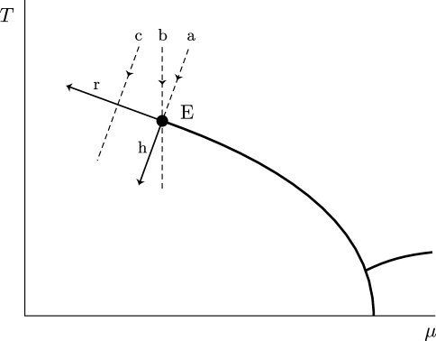
Figure 1: Sketch of the QCD phase diagram as a function of temperature $T$ and baryon chemical potential $\mu$. Chiral symmetry is broken at low $T$ and $\mu$. As $T$ is increased, chiral symmetry is approximately restored via a smooth crossover to the left of $E$ or a first order phase transition to the right of $E$. The symmetry is only approximately restored because the light quarks are not massless. At the critical point $E$ at which the line of first order phase transitions ends, the transition is second order and is in the Ising universality class. (At large $\mu$ and small $T$, there are color superconducting phases which we do not discuss in this paper.) The Ising model $r$-axis and $h$-axis and the trajectories a, b and c will be discussed in Section 2.

Arguments based on a variety of models [7, 8, 9, 10, 11, 12, 13, 14] indicate that the transition as a function of $T$ is first order at large $\mu$. This suggests that the phase diagram features a critical point $E$ at which the line of first order phase transitions present for $\mu>\mu_{E}$ ends, as shown in Figure 1. At $\mu_{E}$, the phase transition at $T=T_{E}$ is second order and is in the Ising universality class [11, 12]. Although the pions remain massive, the correlation length in the $\sigma$ channel diverges due to universal long wavelength fluctuations of the order parameter. This results in characteristic signatures, analogues of critical opalescence in the sense that they are unique to collisions which freeze out near the critical point, which can be used to discover $E$ [1, 2].

The position of the critical point is, of course, not universal. Furthermore, it is sensitive to the value of the strange quark mass. $\mu_{E}$ decreases as $m_{s}$ is decreased [1], and at some $m_{s}^{c}$, it reaches $\mu_{E}=0$ and the transition becomes entirely first order [15]. The value of $m_{s}^{c}$ is an open question, but lattice simulations suggest that it is about half the physical strange quark mass [16, 17], although these results are not yet conclusive [18]. Of course, experimentalists cannot vary $m_{s}$. They can, however, vary $\mu$. The AGS, with beam energy 11 AGeV corresponding to $\sqrt{s}=5$ GeV, creates fireballs which freeze out near $\mu\sim 500-600$ MeV [19]. When the SPS runs with $\sqrt{s}=17$ GeV (beam energy 158 AGeV), it creates fireballs which freeze out near $\mu\sim 200$ MeV [19]. RHIC will make even smaller values of $\mu$ accessible. By dialing $\sqrt{s}$ and thus $\mu$, experimenters can find the critical point $E$.

1.2 Detecting the Critical Point

Predicting $\mu_{E}$, and thus suggesting the $\sqrt{s}$ to use to find $E$, is beyond the reach of present theoretical methods because $\mu_{E}$ is both nonuniversal and sensitively dependent on the mass of the strange quark. Crude models suggest that $\mu_{E}$ could be $\sim 600-800$ MeV in the absence of the strange quark [11, 12]; this in turn suggests that in nature $\mu_{E}$ may have of order half this value, and may therefore be accessible at the SPS if the SPS runs with $\sqrt{s}<17$ GeV. However, at present theorists cannot predict the value of $\mu_{E}$ even to within a factor of two. The SPS can search a significant fraction of the parameter space; if it does not find $E$, it will then be up to the RHIC experiments to map the $\mu_{E}<200$ MeV region.

Locating $E$ on the phase diagram can only be done convincingly by an experimental discovery. Theorists can, however, do reasonably well at describing the phenomena that occur near $E$, thus enabling experimenters to locate it. This is the goal of Ref. [2]. The signatures proposed there are based on the fact that $E$ is a genuine thermodynamic singularity at which susceptibilities diverge and the order parameter fluctuates on long wavelengths. The resulting signatures are nonmonotonic as a function of $\sqrt{s}$: as this control parameter is varied, we should see the signatures strengthen and then weaken again as the critical point is approached and then passed.

The simplest observables to use are the event-by-event fluctuations of the mean transverse momentum of the charged particles in an event, $p_{T}$, and of the total charged multiplicity in an event, $N$. One analysis described in detail in Ref. [2] is based on the ratio of the width of the true event-by-event distribution of the mean $p_{T}$ to the width of the distribution in a sample of mixed events. This ratio was called $\sqrt{F}$. NA49 has measured $\sqrt{F}=1.002\pm 0.002$ [20, 2], which is consistent with expectations for noncritical thermodynamic fluctuations. Critical fluctuations of the $\sigma$ field, i.e. the characteristic long wavelength fluctuations of the order parameter near $E$, influence pion momenta via the (large) $\sigma\pi\pi$ coupling and increase $\sqrt{F}$ [2]. The effect is proportional to $\xi_{\rm freezeout}^{2}$, where $\xi_{\rm freezeout}$ is the $\sigma$-field correlation length of the long-wavelength fluctuations at freezeout [2]. If $\xi_{\rm freezeout}\sim 6$ fm, the ratio $\sqrt{F}$ increases by $10-20\%$, fifty times the statistical error in the present measurement [2]. This observable is valuable because data on it has been analyzed and presented by NA49, and it can therefore be used to learn that Pb+Pb collisions at 158 AGeV do not freeze out near $E$.

Once $E$ is located, however, other observables which are more sensitive to critical effects will be more useful. For example, a $\sqrt{F_{\rm soft}}$, defined using only the softest $10\%$ of the pions in each event, will be much more sensitive to the critical long wavelength fluctuations. The higher $p_{T}$ pions are less affected by the $\sigma$ fluctuations [2], and these relatively unaffected pions dominate the mean $p_{T}$ of all the pions in the event. This is why the increase in $\sqrt{F}$ near the critical point will be much less than that of $\sqrt{F_{\rm soft}}$.

The multiplicity of soft pions is an example of an observable which may be used to detect the critical fluctuations without an event-by-event analysis. The post-freezeout decay of sigmas, which are copious and light at freezeout near $E$ and which decay subsequently when their mass increases above twice the pion mass, should result in a population of pions with $p_{T}\sim m_{\pi}/2$ which appears only for freezeout near the critical point [2]. If $\xi_{\rm freezeout}\gtrsim 1/m_{\pi}$, this population of unusually low momentum pions will be comparable in number to that of the “direct” pions (i.e. those which were pions at freezeout) and will result in a large signature.

The variety of observables which should all show nonmonotonic behavior near the critical point is sufficiently great that if it were to turn out that $\mu_{E}<200$ MeV, making $E$ inaccessible to the SPS, all four RHIC experiments could play a role in the study of the critical point.

1.3 How Large Can $\xi$ Grow?

Our purpose in this paper is to estimate how large $\xi_{\rm freezeout}$ can become, thus making the predictions of Ref. [2] for the magnitude of various signatures more quantitative. In an ideal system of infinite size which was held at $T=T_{E}$; $\mu=\mu_{E}$ for an infinite time, the correlation length $\xi$ would be infinite. Ref. [2] estimated that finite size effects limit $\xi$ to be about 6 fm at most. We will argue in this paper that limitations imposed by the finite duration of a heavy ion collision are more severe, preventing $\xi$ from growing larger than about $2/T_{E}\sim 3$ fm.

1.4 $T_{E}$, $T_{\rm freezeout}$, and $T_{0}$

We will do the calculation in the next section in the three-dimensional Ising model, as appropriate for describing the universal dynamics of the long wavelength fluctuations near the critical point. However, in order to relate a calculation in the Ising model to experiments which explore the QCD phase diagram, we will need numerical values for three temperature scales. Several other nonuniversal quantities will also enter our calculation; we will discuss them in the next section as they arise. We will see that in the end, only one combination of nonuniversal quantities plays a role in our estimates.

We expect $T_{E}$ to be slightly less than the temperature range at which the crossover occurs at $\mu=0$. We therefore take $T_{E}=140$ MeV, at the low end of lattice estimates for the $\mu=0$ crossover temperature.

As we have discussed at length, we know very little about $\mu_{E}$. Fortunately, we will not need a numerical value for $\mu_{E}$ below.

Pb+Pb collisions at 158 AGeV freeze out at about 120 MeV, and NA49 data [20] demonstrate clearly that they do not freeze out near $E$ [2]. We also know [1] that if the matter produced in a heavy ion collision comes near $E$, the large specific heat characteristic of $E$ will cause the system to “linger” — the expansion will cause the energy density to decrease as usual, but this will result in an unusually slow temperature decrease. The freezeout temperature is therefore expected to be unusually close to the critical temperature for collisions which have the appropriate $\mu$ to pass near $E$. For concreteness, we will take $T_{\rm freezeout}=130$ MeV. (If the freeze-out temperature in Pb+Pb collisions at 158 AGeV is closer to 100 MeV, as some authors estimate [24], then it may be better to estimate that collisions which pass near $E$ freezeout at $T_{\rm freezeout}=120$ MeV.)

Finally, we need to estimate $T_{0}$, the temperature at which we can begin an Ising model treatment. The three dimensional Ising model is only valid close enough to $E$ that the correlation length $\xi>1/T_{E}$. In this critical region, the long wavelength fluctuations of the order parameter become effectively three dimensional. (We will find that $\xi$ is never $\gg 1/T_{E}$. This means that our estimates are not precise.) We need to know how far above $T_{E}$ the equilibrium correlation length is larger than $1/T_{E}$. The model of Ref. [11] suggests that $\xi_{\rm eq}>1/T_{E}$ for $(T-T_{E})/T_{E}\lesssim 0.2-0.4$. This estimate is based on a mean field analysis of a toy model, and so should not be taken too seriously. For concreteness we shall assume that $\xi_{\rm eq}=1/T_{E}\equiv\xi_{0}$ at $T_{0}=180$ MeV, 40 MeV above $T_{E}\sim 140$. We will use $\xi_{0}=1.4$ fm to set the scale below, in the sense that we will estimate the factor by which $\xi/\xi_{0}$ grows as the system cools. $\xi_{0}=1.4$ fm is simply a definition; $T_{0}$, the temperature at which the equilibrium correlation length $\xi_{\rm eq}=\xi_{0}$, is a quantity which must be estimated and which will affect our results.

2 Slowing Out of Equilibrium

The nonequilibrium dynamics which we analyze in this paper is fundamental in the sense that it is guaranteed to occur in a heavy ion collision which passes near $E$, even if local thermal equilibrium is achieved at a higher temperature during the earlier evolution of the plasma created in the collision. We assume early thermal (although not necessarily chemical) equilibration, and ask how the system evolves out of equilibrium as it passes $E$. More precisely, we will assume that when the system has cooled to $T=T_{0}=180$ MeV, it is in equilibrium, with $\xi(T_{0})=\xi_{\rm eq}(T_{0})=\xi_{0}$. For the present, assume that the system cools through the critical point $E$, as sketched in trajectory (a) of Figure 1. If it were to cool arbitrarily slowly, $\xi=\xi_{\rm eq}$ would be maintained at all temperatures, and $\xi$ would diverge at $T_{E}$. However, it would take an infinite time for $\xi$ to grow infinitely large. Indeed, near a critical point, the long correlation length results in long equilibration times, a phenomenon known as critical slowing down. This means that the correlation length cannot grow as fast as $\xi_{\rm eq}$, and the system cannot stay in equilibrium.

We describe the effects of critical slowing down on the time development of the correlation length $\xi(t)$ using the following equation for $m_{\sigma}(t)\equiv 1/\xi(t)$:

$$\frac{d}{dt}\,m_{\sigma}(t)=-\Gamma\left(m_{\sigma}(t)\right)\left(m_{\sigma}(t)-\frac{1}{\xi_{\rm eq}(t)}\right)\ .$$ (2.1)

Here, $\Gamma$ parametrizes the rate at which an out-of-equilibrium value of $m_{\sigma}$ approaches its equilibrium value. If $m_{\sigma}$ is close to its equilibrium value, the theory of dynamical critical phenomena [25] tells us that

$$\Gamma(m_{\sigma})=\frac{A}{\xi_{0}}\,\left(m_{\sigma}\xi_{0}\right)^{z}$$ (2.2)

where $z$ is a universal exponent and we have used $\xi_{0}$ to set the scale, making $A$ a dimensionless constant. Knowing that we are interested in a system which is in the same static universality class as the 3-dimensional Ising model is not enough to tell us $z$. There are in general several different dynamical universality classes corresponding to a given static universality class. However, knowing in addition that: (i) the chiral order parameter is not a conserved quantity; (ii) there are other conserved quantities in the system, like the baryon number density; and (iii) there are no Poisson bracket relations between the order parameter and the conserved quantities, tells us that our system belongs in the dynamical universality class named Model C in Halperin and Hohenberg’s classification [25] of dynamical critical phenomena, and has

$$z=2+\alpha/\nu\approx 2.17\ ,$$ (2.3)

where we have taken $\alpha=0.11$ and $\nu=0.630$ from Ref. [26]. The dimensionless constant $A$ is nonuniversal. We have no way to estimate it other than to guess that it is of order 1. We will explore the sensitivity of our results to different choices of $A$ below.

We will use the differential equation (2.1) to analyze how critical slowing down prevents the correlation length $\xi$ from “tracking” $\xi_{\rm eq}(T(t))$. Critical slowing down guarantees that the system falls out of equilibrium. Note that the differential equation has only been derived for small departures from equilibrium; once $m_{\sigma}-\xi_{\rm eq}^{-1}$ is not small, its use is not quantitatively justified.

We have initial conditions for the differential equation (2.1), namely $m_{\sigma}(0)=1/\xi_{0}$. Therefore, all we need in order to solve it is a description of $\xi_{\rm eq}(t)$. This requires $\xi_{\rm eq}(T)$, which we discuss below, and also requires a description of the cooling $T(t)$. This can be estimated using hydrodynamic and cascade model calculations, although these describe $T(t)$ assuming the plasma is not cooling near the critical point $E$. Hydrodynamic models (see, e.g., Refs. [23, 27]) describe $T(t)$ at central rapidity in the center of mass frame via

$$\frac{dT}{dt}=-\frac{1}{\kappa}\frac{T}{t_{0}}\ .$$ (2.4)

Since we are only interested in a relatively small range of temperatures around $T_{E}$, it will suffice for us to treat $dT/dt$ as constant in time. We discuss the effects of the time dependence of $dT/dt$ below. The expression (2.4) assumes that the $T$-dependence of the energy density is $\epsilon\sim T^{\kappa}$ as in a resonance gas, for which $\kappa\approx 6$ [28]. The timescale $t_{0}$ is not constant over the whole history of the collision. A simplified estimate (made by equating $t_{0}$ with the scattering time) suggests that in Pb+Pb collisions at 158 AGeV, $t_{0}$ is between 4 and 10 fm at times of interest to us [27]. This suggests $-dT/dt=(2-6){\rm~{}MeV}/{\rm fm}$ at $T=140$ MeV. Careful analysis favors $t_{0}$ closer to $4$ fm [24]. This agrees with a recent analysis of these collisions using the URQMD cascade model, which suggests $-dT/dt\approx 5{\rm~{}MeV}/{\rm fm}$ at $T=140$ MeV [29]. These estimates are all for cooling through $T=140$ MeV at a $\mu$ such that one is not near the critical point. As we discussed above, the cooling rate is likely to be unusually low near $E$ because of the large specific heat there; we will therefore take $-dT/dt\sim 4{\rm~{}MeV}/{\rm fm}$ as our estimate, noting also that the cooling rate at RHIC will be slower still.

We wish to use the three-dimensional Ising model to describe $\xi_{\rm eq}(T,\mu)$ near $E$. In the Ising model, the order parameter $M$ (the magnetization) and the correlation length $\xi$ are functions of the reduced temperature $r$ and the magnetic field $h$. (In the Ising model, $r$ is defined as $(T-T_{c})/T_{c}$ and is usually called $t$; we reserve the symbol $t$ for time, however.) The critical point is at $r=h=0$; at this point, $M=0$ and $\xi_{\rm eq}=\infty$. For $r<0$, there is a first order phase transition as a function of $h$ at $h=0$ between $M=|r|^{\beta}$ for $h=0+$ and $M=-|r|^{\beta}$ for $h=0-$. The exponent is $\beta=0.326$ for the 3-dimensional Ising model [26]. For $r>0$, $M$ increases smoothly through zero as $h$ goes from negative to positive. For $r=0$, the order parameter is $M={\rm sign}(h)|h|^{1/\delta}$, with $\delta=4.80$ [26].

We can now discuss how the Ising model $r$- and $h$-axes are mapped onto the $(T,\mu)$ plane. The $r$-axis is the direction tangential to the line of first order phase transitions ending at $E$. This is shown in Figure 1. There is no guarantee that the $h$-axis is perpendicular to the $r$-axis when both are mapped onto the $(T,\mu)$ plane. This mapping will in general deform the Ising axes, but we have no way of estimating this deformation. For simplicity, we draw the $h$-axis perpendicular to the $r$-axis in Figure 1. In thinking through the mapping between QCD and the Ising model even qualitatively, it is important to note that the QCD order parameter ( the chiral condensate $\langle\bar{q}q\rangle$) is offset with respect to the Ising model order parameter (the magnetization $M$). In the Ising model, $M=0$ at the critical point and along the first order line one has phase coexistence between phases whose $M$’s are equal in magnitude and opposite in sign. In QCD, $\langle\bar{q}q\rangle\neq 0$ at the critical point $E$, because of the explicit breaking of the $O(4)$ symmetry by quark mass terms. Near $E$, $\langle\bar{q}q\rangle$ corresponds to $M$ plus an offset, and the phase coexistence is between phases with differing values of $\langle\bar{q}q\rangle$ which both have the same sign. In Figure 1, we take the $-h$ side of the Ising coexistence line to correspond to the higher temperature side of the QCD coexistence line, so that increasing $M$ corresponds to increasing the magnitude of $\langle\bar{q}q\rangle$.

The matter created in heavy ion collisions at SPS energies will follow a trajectory in the $(T,\mu)$ plane which is approximately vertical as it cools. (See, for example, Ref. [29].) We therefore begin by considering trajectory (a) of Figure 1, which follows the $h$-axis, as this is likely not a bad approximation to cooling at almost constant $\mu$. We have analyzed trajectories which pass through $E$ at a variety of angles, for example like trajectory (b) in Figure 1. The results do not differ qualitatively from those we present in detail for a trajectory along the $h$-axis, unless the trajectory passes through $E$ almost parallel to the $r$-axis. At the end of this section, we will present results for trajectories like (c) in Figure 1, which miss $E$ but come close to it.

Let us take the initial temperature in our calculation, $T=T_{0}=180$ MeV, to correspond to $h=h_{0}=-0.2$. Along the $h$-axis, as in trajectory (a), the equilibrium correlation length is a power law in $h$:

$$\xi_{\rm eq}(h)=\left|\frac{h}{h_{0}}\right|^{-\nu/\beta\delta}\ ,$$ (2.5)

where we have normalized $\xi$ by setting $\xi_{\rm eq}(h_{0})=1$. That is, we measure $\xi$ in units of $\xi_{0}=1.4$ fm. With units chosen, we can now rewrite the equation (2.1) which describes the dynamics of the growth of the correlation length $\xi=1/m_{\sigma}$ in terms of Ising model variables as

$$\frac{d}{dh}\,m_{\sigma}(h)=-a\,\Biggl{(}m_{\sigma}(h)\Biggr{)}^{z}\,\left(m_{\sigma}(h)-\frac{1}{\xi_{\rm eq}(h)}\right)$$ (2.6)

where the nonuniversal constant $a$ is related to the other nonuniversal parameters we have discussed by:

$$a=A\left(\frac{dh}{dt}\right)^{-1}=A\left(\frac{h_{0}}{T_{0}-T_{E}}\frac{dT}{dt}\right)^{-1}\ .$$ (2.7)

Nonuniversal parameters appear in equation (2.6) only in the single combination $a$. Taking the nonuniversal constant from (2.2) to be $A\sim 1$, using $(T_{0}-T_{E})=40$ MeV, $dT/dt=-4{\rm~{}MeV}/{\rm fm}$ and $h_{0}=-0.2$ yields the estimate

$$a\sim 50\ .$$ (2.8)

In fact, because $\xi_{\rm eq}(h)$ is a power law in $h$, if one changes $h_{0}$ and then redefines the units of $\xi$ so that $\xi_{\rm eq}(h_{0})$ is again set to one, equation (2.6) is unaffected. Our results are therefore determined solely by $A$, $(T_{0}-T_{E})$ and $dT/dt$ in the single combination $a$, together with the assumption that the system begins in equilibrium at $T=T_{0}$.

Figure 2: Behavior of the correlation length for cooling through the critical point along the $h$-axis of Figure 1. The equilibrium correlation length is shown as a dashed line. The true correlation length is shown for (bottom to top) $a=25,50,100$. Our units, described in the text, are such that $h=-0.2,-0.1,0,0.1$ corresponds to $T=180,160,140,120$ MeV, and $\xi$ is measured in units of $\xi_{0}=1.4$ fm.

We can now use (2.6) to learn how much $\xi$ grows relative to $\xi_{0}=1.4$ fm. Given the uncertainties in the determination of $a$, in Figure 2 we show $\xi(h)$ obtained by solving (2.6) for $a=25,50,100$. Four lessons are apparent:

First, critical slowing down has a large effect. Although by assumption we begin in thermal equilibrium with $\xi=\xi_{\rm eq}$ at $T=T_{0}$, the fact that the dynamics slows down in the vicinity of $E$ prevents $\xi$ from tracking $\xi_{\rm eq}$ and growing very large.

Second, our results do not depend sensitively on the parameter $a$. This is fortunate, since there are so many uncertainties involved in estimating $a$. For $a=25,50,100$, the maximum correlation length which is achieved is $1.8\xi_{0}$, $2.1\xi_{0}$, $2.5\xi_{0}$, corresponding to 2.6, 3.0, 3.4 fm. This means that although our estimate is only qualitative, it is clear that $\xi$ cannot grow as large as 6 fm. (To obtain a maximum value of $\xi=4\xi_{0}$ would require $a=1000$. Although $a$ is uncertain, this large a value seems out of the question.) We estimate that $\xi$ grows to about twice $\xi_{0}$, corresponding to approximately 3 fm.

Third, since previous work [2] suggests that finite size effects limit $\xi$ to $\xi<6$ fm, we conclude that slowing out of equilibrium (i.e. the combination of finite time and critical slowing down) imposes the more stringent constraint on $\xi$. We have analyzed this nonequilibrium effect as if the system were spatially homogeneous. Had we found correlation lengths growing beyond 6 fm, we would have to do a much more complicated analysis, taking both the finite time and the inhomogeneous spatial dynamics into account. Since we find that $\xi$ only grows to about 3 fm, this is not necessary.

Fourth, just as critical slowing down prevents $\xi$ from growing as fast as $\xi_{\rm eq}$ does, it also prevents $\xi$ from shrinking as fast as $\xi_{\rm eq}$ does after $E$ has been passed. Whether we estimate $T_{\rm freezeout}\sim 130$ MeV (corresponding to $h=.05$) or $\sim 120$ MeV ($h=0.1$) for trajectories passing near $E$, one finds $\xi_{\rm freezeout}\sim 2\xi_{0}$. We can also argue that even if an $a$ as large as 1000 were possible, our conclusions would be little affected: If $a=1000$, and $\xi$ follows $\xi_{\rm eq}$ closely enough that it increases to $4\xi_{0}$, $\xi$ also tracks $\xi_{\rm eq}$ more closely as it decreases below $T_{E}$. If $a=1000$, it turns out that $\xi$ is quite close to $\xi_{\rm eq}$ by the time $h=.05$. Thus, although increasing $a$ to a ridiculous extent does increase the maximum value of $\xi$, it has little effect on $\xi_{\rm freezeout}$. This is further evidence that although our estimate $\xi_{\rm freezeout}\sim 2\xi_{0}\sim 3$ fm is qualitative, it is robust.

The $a$-dependence of the maximum value attained by $\xi$ can be understood analytically at large $a$. For large $a$, $m_{\sigma}$ tracks its equilibrium value $m_{\sigma}^{\rm eq}=|h/h_{0}|^{\nu/\beta\delta}$ well until $|h/h_{0}|$ is quite small. If we define $\epsilon\equiv m_{\sigma}-m_{\sigma}^{\rm eq}$, we can use (2.6) to show that $\epsilon<m_{\sigma}^{\rm eq}$ as long as

$$\frac{h}{h_{0}}>\left(\frac{\nu}{\beta\delta}\frac{1}{a}\right)^{\frac{1}{1+z\nu/\beta\delta}}\ .$$ (2.9)

If we assume that once $\xi$ begins to drop out of equilibrium (i.e. once $\epsilon$ begins to grow comparable to $m_{\sigma}^{\rm eq}$), little further growth of $\xi$ occurs before $\xi$ reaches its maximum, we predict that $\xi$ will peak at

$$\xi^{\rm max}=\left(c\,a\right)^{\frac{\nu/\beta\delta}{1+z\nu/\beta\delta}}=\left(c\,a\right)^{0.215}\ ,$$ (2.10)

for some constant $c$. The maxima of solutions to (2.6) obtained numerically follow this scaling relation (with $c=0.65$) quite accurately once $a>1000$ or so. Even at much smaller $a$, as in Figure 2, $\xi^{\rm max}$ is within a few percent of that in (2.10). This scaling relation explains why our results are so weakly dependent on $a$. Note that even with the scaling relation in hand, full solutions as in Figure 2 are of value because they allow us to estimate $\xi_{\rm freezeout}$ and not just $\xi_{\rm max}$.

We have to this point assumed that $dT/dt$ is approximately constant as the system cools through $T_{E}$. This is an oversimplification. It is more reasonable to assume that $ds/dt$ is approximately constant, where $s$ is the entropy density. Since

$$\frac{dT}{dt}=\frac{1}{C_{V}}\frac{ds}{dt}\$$ (2.11)

and the specific heat $C_{V}$ is peaked at $T_{E}$, we expect that $dT/dt$ is unusually small near $T_{E}$. As we discussed above, this “lingering” results in a $T_{\rm freezeout}$ which is unusually close to $T_{E}$ [1]. Here, we estimate the effect of lingering near $E$ on the growth of $\xi$. Along the $h$-axis, the specific heat due to the long wavelength sigma fluctuations diverges like $C_{V}\sim h^{-\gamma/\beta\delta}\sim\xi_{\rm eq}^{\gamma/\nu}$ in thermal equilibrium [1]. The exponent $\gamma=1.240$ [26]. We take $C_{V}=c_{1}+c_{2}\xi^{\gamma/\nu}$, where $c_{1}$ is the specific heat due to all the degrees of freedom other than the sigma and is smooth near $T_{E}$. Note that $C_{V}$ depends on the actual correlation length $\xi$, and not on $\xi_{\rm eq}$. In our dynamical nonequilibrium setting, therefore, $C_{V}$ peaks but does not diverge. We can implement lingering in our calculation by replacing the constant $a$ in (2.6) by

$$a(h)=a\left[(1-b)+b\left[m_{\sigma}(h)\right]^{-\gamma/\nu}\right]\ .$$ (2.12)

Here, $a$ is the same constant as before and the constant $b=c_{2}/(c_{1}+c_{2})$ is the fraction of the specific heat at $T=T_{0}$ which is due to sigma fluctuations. This fraction is perhaps about $0.1$ and is surely less than $0.25$. As the system cools from $T_{0}$ to $T_{E}$, the sigma contribution to $C_{V}$ grows and peaks. We find that changing constant $a$ to $a(h)$ as in (2.12) with $b=0.25$ increases $\xi_{\rm max}$ by about $10\%$ beyond that shown in Figure 2, and increases $\xi_{\rm freezeout}$ by somewhat less. For $b=0.1$, the increase in $\xi_{\rm max}$ is about $5\%$. We conclude that because $C_{V}$ receives contributions from all degrees of freedom and not just from the sigma fluctuations, and because $C_{V}$, like $\xi$, peaks but does not diverge, the reduction in $dT/dt$ near $E$ is not large enough to significantly increase $\xi$ beyond our previous estimates.

We now ask how much our results change if we consider trajectories like (c) in Figure 1 which come close to, but miss, $E$. Our analysis can easily be extended to cover those trajectories which pass $E$ on the crossover side ($r>0$; $T<T_{E}$). In an appendix, we present the Ising model expression for $\xi_{\rm eq}(r,h)$ near the critical point. We use this expression to evaluate $\xi(h)$ for trajectories parallel to the $h$-axis with $r=0.12$, $r=0.19$ and $r=0.33$, for which $\xi_{\rm eq}$ peaks at $4\xi_{0}$, $3\xi_{0}$ and $2\xi_{0}$. The results are shown in Figure 3 in which we have taken $a=50$. Note that in plotting Figure 3 we have defined $\xi_{0}=\xi(r,h_{0})=1$ anew for each $r$. We see that as long as $\xi_{\rm eq}$ peaks at $3\xi_{0}$ or higher, the dynamics of $\xi$ is almost the same as for the trajectory of Figure 2 which goes precisely through $E$. Even for a trajectory which misses $E$ by enough that $\xi_{\rm eq}$ peaks at only $2\xi_{0}$, the actual correlation length $\xi$ grows by a factor which is within $20\%$ of that for trajectories which pass arbitrarily close to $E$. Just as the growth of $\xi$ is robust with respect to changes in $a$, it is robust with respect to how close the trajectory comes to $E$, for those trajectories which come close enough.

Figure 3: The dashed curves show $\xi_{\rm eq}(h)$ for trajectories with (top to bottom) $r=0.12,\ 0.19,\ 0.33$. The solid curves show the corresponding nonequilibrium correlation lengths $\xi$, assuming $a=50$. Curves with different $r$ have each been normalized to begin at $\xi(h_{0})=1$.

Our analysis is not sufficient to describe the dynamics for those trajectories which pass to the first order side of $E$, because we do not treat the dynamics of bubble nucleation and phase coexistence. Near enough to $E$, though, the first order transition is so weak that it will not have detectable effects given the finite length and time scales in a heavy ion collision, and the physics is likely qualitatively similar to that we have analyzed on the crossover side of $E$. Farther from $E$ on the first order side, this is not the case. Farther from $E$, though, the correlation length is never large.

3 Consequences

Our results have a number of consequences which should be taken into account both in planning experimental searches for the QCD critical point, and in planning future theoretical work.

Because of critical slowing down, the correlation length in a heavy ion collision cannot grow as fast as it would in equilibrium; this means that $\xi_{\rm freezeout}$ is likely about 3 fm for trajectories passing near $E$. Although finite size effects alone would allow a correlation length as large as 6 fm, this is unrealistic to expect in a heavy ion collision. This effect arises due to guaranteed nonequilibrium physics: even if heavy ion collisions achieve local thermal equilibrium above the transition, as we have assumed, if they cool through the transition near the critical point they must “slow out of equilibrium.” By this we mean that the correlation length cannot grow as it would in equilibrium, because the long wavelength dynamics are slow near $E$.

Critical slowing down also prevents the correlation length from decreasing quickly after passing the critical point. One therefore need not worry about $\xi$ decreasing significantly between the phase transition and freezeout.

One need not hit $E$ precisely in order to find it. The results shown in Figure 3 demonstrate that if one were to do a scan with collisions at many finely spaced values of the energy and thus $\mu$, one would see signatures of $E$ with approximately the same magnitude over a broad range of $\mu$. The magnitude of the signatures will not be narrowly peaked as $\mu$ is varied. As long as one gets close enough to $E$ that the equilibrium correlation length is $(2-3)\xi_{0}$, the actual correlation length $\xi$ will grow to $\sim 2\xi_{0}$. There is no advantage to getting closer to $E$, because critical slowing down prevents $\xi$ from getting much larger even if $\xi_{\rm eq}$ does. Data at many finely spaced values of $\mu$ is not called for.

Only one combination of the nonuniversal quantities (called $a$ above) plays an important role in estimating the dynamics of $\xi$. The uncertainty in $a$ is the sum of that in its three factors: $A$ (the nonuniversal constant in the dynamical scaling law (2.2)), $dT/dt$ and $T_{0}-T_{E}$. It is already fortunate that only one combination $a$ matters; it is even more fortunate that our results are not very sensitive to the value of $a$. This means that although our results are not completely quantitative, they are robust. In addition to the uncertainty in $a$, however, our results cannot be treated as precise because the QCD dynamics are precisely described by the three-dimensional Ising model dynamics only if $\xi\gg 1/T_{E}$, and we have found that $\xi$ does not grow beyond $\sim 2/T_{E}$.

There are a number of steps that could be taken in future work to refine our estimate. One could do a more complete job of analyzing the universal dynamics of a system which passes near an Ising critical point. For example, instead of simply writing a differential equation for $\xi$, one could follow the full 3+1-dimensional dynamics in a Langevin simulation, from which one would measure $\xi$. Doing this, however, would still leave one facing the same nonuniversal uncertainties which we face in our treatment. If we simply ask how to reduce the uncertainty in $a$, perhaps the hardest part of this task would be a reliable calculation of $A$, as that would require a reliable calculational method for QCD dynamics at nonzero $T$ and $\mu$. The other two ingredients in $a$ are likely to become better known as the modeling of heavy ion collisions and the analysis of data from these collisions proceed. It seems, though, that the uncertainty in $A$ will prevent a fully quantitative calculation of $a$ for the foreseeable future. Our results are sufficiently insensitive to $a$ that they suffice to estimate the magnitude of signatures; when these signatures are found, perhaps they will give us more quantitative information about the nonuniversal quantities which go into $a$.

Knowing that we are looking for $\xi_{\rm freezeout}\approx 3$ fm is very helpful in suggesting how to employ the signatures described in detail in Ref. [2]. The excess of pions with $p_{T}\sim m_{\pi}/2$ arising from post-freezeout decay of sigmas is large as long as $\xi_{\rm freezeout}\sim 1/m_{\pi}$, and does not increase much further if $\xi_{\rm freezeout}$ is longer. This makes it an ideal signature. The increase in the event-by-event fluctuations in the mean transverse momentum of the charged pions in an event (described by the ratio $\sqrt{F}$ of Ref. [2]) is proportional to $\xi_{\rm freezeout}^{2}$. The results of Ref. [2] suggest that for $\xi_{\rm freezeout}\sim 3$ fm, this will be a $3-5\%$ effect. This is ten to twenty times larger than the statistical error in the present NA49 data, but not so large as to make one confident of using this alone as a signature for $E$. The solution is to use signatures which focus on the event-by-event fluctuations of only the low momentum pions. Unusual event-by-event fluctuations in the pion momenta arise via the coupling between the pions and the sigma order parameter which, at freezeout, is fluctuating with correlation length $\xi_{\rm freezeout}$. This interaction has the largest effect on the softest pions [2]. $\sqrt{F_{\rm soft}}$, described in the introduction, is a good example of an observable which takes advantage of this. Depending on the details of the cuts used to define it, it should be enhanced by many tens of percent in collisions passing near $E$. Ref. [2] suggests other such observables, and more can surely be found. Together, the excess multiplicity at low momentum (due to post-freezeout sigma decays) and the excess event-by-event fluctuation of the momenta of the low momentum pions (due to their coupling to the order parameter which is fluctuating with correlation length $\xi_{\rm freezeout}$) should allow a convincing detection of the critical point $E$. Both should behave nonmonotonically as the collision energy, and hence $\mu$, are varied. Both should peak for those heavy ion collisions which freeze out near $E$, with $\xi_{\rm freezeout}\sim 3$ fm.

Acknowledgments

We acknowledge helpful conversations with J. Bowers, B. Halperin, U. Heinz, E. Shuryak and M. Stephanov. This work is supported in part by the U.S. Department of Energy (D.O.E.) under cooperative research agreement #DF-FC02-94ER40818. The work of KR is supported in part by a DOE OJI Award and by the Alfred P. Sloan Foundation.

Appendix A Equilibrium Correlation Length

In this appendix we present the equations that we used to calculate the equilibrium correlation length $\xi_{\rm eq}$ in the critical region as a function of reduced temperature $r$ and external magnetic field $h$. We use Widom’s scaling form [32]

$$\xi_{\rm eq}^{2}(r,M)=f^{2}\,M^{-2\nu/\beta}g\left({|r|\over|M|^{1/\beta}}\right),$$ (A.1)

in which $M$ is the magnetization and $\nu=0.630$ and $\beta=0.326$ are the three-dimensional Ising model critical exponents [26]. The $\varepsilon$-expansion of $g(x)$ is given in [32] to order $\varepsilon^{2}$:

$$g(x)=g_{\varepsilon}(x) = 6^{-2\nu}z\Biggl{\{}1-{\varepsilon\over 36}\left[(5+6\ln 3)z-6(1+z)\ln z\right]+$$

$$\varepsilon^{2}\Biggl{[}{1+2z^{2}\over 72}\ln^{2}z+\Bigl{(}{z\over 18}(z-{1\over 2})(1-\ln 3)-$$

$${1\over 216}(16z^{2}-{47\over 3}z-{56\over 3})\Bigr{)}\ln z+$$

$${1\over 216}\Bigl{(}{101\over 6}+{2\over 3}I+6\ln^{2}3+4\ln 3-10\Bigr{)}z^{2}-$$

$${1\over 216}\Bigl{(}6\ln^{2}3+{44\over 3}\ln 3+{137\over 9}+{8\over 3}I\Bigr{)}z\Biggr{]}\Biggr{\}},$$

$$\mbox{where }z \equiv {2\over 1+{x\over 3}},\mbox{ and }I=\int_{0}^{1}{\ln\left[x(1-x)\right]\over 1-x(1-x)}dx\approx-2.344.$$

$f$ in (A.1) is a non-universal normalization constant, often set to one. Our choice of $f$ and thus of units for $\xi$ is described in Section 2. The expression (A.2) is valid everywhere on the ($r,M$) plane except the region of large $x$ (or, equivalently, $r\gg|M|^{1/\beta}$). The correct result at large $x$ is

$$g_{\rm large}(x)=\left({1\over 3+x}\right)^{2\nu},$$ (A.3)

and we therefore construct a function $g(x)$ which smoothly interpolates between $g_{\rm large}(x)$ at large $x$ and $g_{\varepsilon}(x)$ at smaller $x$. The only remaining difficulty is at $r\geq 0$, $M=0$. Although the scaling form (A.1) with (A.3) is well-behaved in the $M\rightarrow 0$ limit, and yields

$$\xi_{\rm eq}(r\geq 0,M\rightarrow 0)=f|r|^{-\nu},$$

at $M=0$ the scaling form is indeterminate and one must impose the condition $\xi_{\rm eq}(r\geq 0,M=0)=\xi_{\rm eq}(r\geq 0,M\rightarrow 0)$.

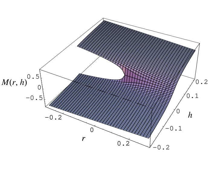
Figure 4: Order parameter (magnetization) in the 3D Ising model as a function of reduced temperature $r$ and applied field $h$.

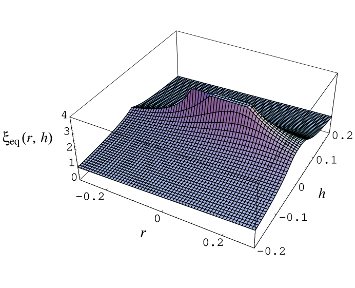
Figure 5: Equilibrium correlation length as a function of reduced temperature $r$ and applied field $h$.

We want $\xi_{\rm eq}(r,h)$. With $\xi_{\rm eq}(r,M)$ in hand, we must now obtain the magnetization $M(r,h)$. The most convenient form for our purposes is the parametric equation of state (see [26, 32, 33]):

$$\left\{\begin{array}[]{ccl}M&=&M_{0}R^{\beta}\theta\\ h&=&h_{0}R^{\beta\delta}\tilde{h}(\theta)=h_{0}R^{\beta\delta}(\theta-0.76201\,\theta^{3}+0.00804\,\theta^{5})\\ r&=&R(1-\theta^{2})\end{array}\right.$$ (A.4)

Here $M$, $r$ and $h$ are parametrized in terms of the “radius” $R\geq 0$ and “polar angle” $\theta$. $\theta=0$ corresponds to $r>0$, $h=0$; $\theta=\pm 1$ corresponds to $r=0$ with positive and negative $h$ respectively. $\tilde{h}(\theta)$ is zero at $\theta=\pm 1.154$, which corresponds to $r<0,h=\pm 0$. The function $\tilde{h}(\theta)$ in (A.4) is from Ref. [26], where it is constructed to be consistent with all that is known from the $\varepsilon$-expansion, from perturbation theory, and from resummations thereof. We choose the normalization constants $M_{0}$ and $h_{0}$ so that $M(r=-1,h=0)=1$ and $M(r=0,h=1)=1$. This guarantees that along the negative $r$ axis $M(r,h=0)=|r|^{-\beta}$ and along the $h$ axis $M(r=0,h)=\mbox{sign}(h)|h|^{-\delta}$. Numerically solving the last two equations of (A.4) for $R$ and $\theta$ in terms of $r$ and $h$, we use the first one to compute $M(r,h)$, shown in Figure 4. This allows us to obtain $\xi_{\rm eq}(r,h)$, shown in Figure 5.

References

- [1] M. Stephanov, K. Rajagopal and E. Shuryak, Phys. Rev. Lett. 81 (1998) 4816.
- [2] M. Stephanov, K. Rajagopal and E. Shuryak, Phys. Rev. D60 (1999) 114028.
- [3] For a recent review, see K. Rajagopal, to appear in Proceedings of Quark Matter ’99, hep-ph/9908360.
- [4] R. Pisarski and F. Wilczek, Phys. Rev. D29 (1984) 338.
- [5] For reviews, see E. Laermann Nucl. Phys. Proc. Suppl. 63 (1998) 114 and A. Ukawa, Nucl. Phys. Proc. Suppl. 53 (1997) 106.
- [6] For example, S. Gottlieb et al., Phys. Rev. D55 (1997) 6852 and R. Mawhinney, talk at ISMD99, Providence, RI, 1999.
- [7] A. Barducci, R. Casalbuoni, S. De Curtis, R. Gatto, G. Pettini, Phys. Lett. B231 (1989) 463; S.P. Klevansky, Rev. Mod. Phys. 64 (1992) 649; A. Barducci, R. Casalbuoni, G. Pettini and R. Gatto, Phys. Rev. D49 (1994) 426.
- [8] M. Stephanov, Phys. Rev. Lett. 76 (1996) 4472; Nucl. Phys. Proc. Suppl. 53 (1997) 469.
- [9] M. Alford, K. Rajagopal and F. Wilczek, Phys. Lett. B422 (1998) 247.
- [10] R. Rapp, T. Schäfer, E. V. Shuryak and M. Velkovsky, Phys. Rev. Lett. 81 (1998) 53.
- [11] J. Berges and K. Rajagopal, Nucl. Phys. B538 (1999) 215.
- [12] M. A. Halasz, A. D. Jackson, R. E. Shrock, M. A. Stephanov and J. J. M. Verbaarschot, Phys. Rev. D58 (1998) 096007.
- [13] R. Pisarski and D. Rischke, Phys. Rev. Lett. 83 (1999) 37.
- [14] G. Carter and D. Diakonov, Phys. Rev. D60 (1999) 016004.
- [15] F. Wilczek, Int. J. Mod. Phys. A7 (1992) 3911; K. Rajagopal and F. Wilczek, Nucl. Phys. B399 (1993) 395.
- [16] F. Brown et al, Phys. Rev. Lett. 65 (1990) 2491.
- [17] JLQCD Collaboration, Nucl. Phys. Proc. Suppl. 73 (1999) 459.
- [18] Y. Iwasaki et al, Phys. Rev. D54 (1996) 7010.
- [19] See, e.g., P. Braun-Munziger and J. Stachel, Nucl. Phys. A606 (1996) 320.
- [20] NA49 Collaboration, hep-ex/9904014.
- [21] St. Mrówczyński, Phys. Lett. B430 (1998) 9.
- [22] The fact that larger systems freezeout later has been established experimentally by seeing the -dependence of the freeze-out temperature via analyses of flow [23], Coulomb effects (H. W. Barz, J. P. Bondorf, J. J. Gaardhoje and H. Heiselberg, Phys. Rev. C57 (1998) 2536), and pion interferometry (U. Heinz, Proceedings of Quark Matter ’97, nucl-th/9801050).
- [23] C. M. Hung and E. Shuryak, Phys. Rev. C57 (1998) 1891.
- [24] B. Tomasik, U. A. Wiedemann and U. Heinz, nucl-th/9907096; and U. Heinz, private communication.
- [25] P. C. Hohenberg and B. I. Halperin, Rev. Mod. Phys. 49 (1977) 435.
- [26] R. Guida and J. Zinn-Justin, hep-th/9610223; cond-mat/9803240; and J. Zinn-Justin hep-th/9810193.
- [27] E. Schnedermann and U. Heinz, Phys. Rev. C47 (1993) 1738; and C50 (1994) 1675; and U. Heinz, private communication.
- [28] E. Shuryak, Sov. J. Nucl. Phys. 16 (1973) 220.
- [29] L. V. Bravina et al, Phys. Rev. C60 (1999) 024904.
- [30] See, e.g., K. Rummukainen, M. Tsypin, K. Kajantie, M. Laine and M. Shaposhnikov, Nucl. Phys. B532 (1998) 283.
- [31] M. Stephanov, private communication.
- [32] E. Brézin, J. C. Le Guillou, and J. Zinn-Justin, in Phase Transitions and Critical Phenomena 6, (Academic Press, 1976), ed. C. Domb and M. S. Green.
- [33] D. Wallace in Phase Transitions and Critical Phenomena 6, (Academic Press, 1976), ed. C. Domb and M. S. Green.