DESCRIPTION OF THE PROTON STRUCTURE FUNCTION $F_{2}^{p}(x,Q^{2})$ IN THE FRAMEWORK OF EXTENDED REGGE - EIKONAL APPROACH

The proton structure function $F_{2}^{p}(x,Q^{2})$ is described in the framework of the off-shell extention of the Regge-eikonal approach which automatically takes into account off-shell unitarity. We achieved a good quality of description for $x<10^{-2}$ and we argue that the data on $F_{2}^{p}(x,Q^{2})$ measured at HERA can be fairly described with classical universal Regge trajectories. No extra, “hard” trajectories of high intercept are needed for that. The $x-,Q^{2}-$ slopes and the effective intercept are discussed as functions of $Q^{2}$ and $x$.

1 INTRODUCTION

In the literature one can find a number of models describing the behaviour of $F_{2}^{p}(x,Q^{2})$in the framework of so called “soft” pomeron $\!{}^{{\bf?}}$ or with help of “hard” pomeron $\!{}^{{\bf?}}$. We add our arguments in favour of the “soft” pomeron by introducing a model taking into account unitarity for the processes with virtual particles. We outline some basic properties of the model that will help to distinguish it from the others.

2 OFF-SHELL EXTENTION OF THE REGGE-EIKONAL APPROACH

Construction of the model starts from the unitarity condition:

$$ImT(s,\vec{b})=|T(s,\vec{b})|^{2}+\eta(s,\vec{b})$$

(here $T(s,\vec{b})$ is the scattering amplitude in the impact representation, $\vec{b}$ is the impact parameter, $\eta(s,\vec{b})$ stands for the contribution of inelastic channels) which in case of eikonal amplitude

$$T(s,\vec{b})=\frac{e^{2i\delta(s,\vec{b})}-1}{2i}$$ (1)

(here $T(s,\vec{b})$ is the scattering amplitude, $\delta(s,\vec{b})$ is the eikonal function), may be rewritten as

$$Im\delta(s,\vec{b})\geq 0,\;s>s_{inel}$$ (2)

We choose the following eikonal function in $t$-space (here $t$ is transferred momentum)

$$\hat{\delta}(s,t)=c\Big{(}\frac{s}{s_{0}}\Big{)}^{\alpha(0)}e^{t\frac{\rho^{2}}{4}}$$ (3)

where

$$\rho^{2}=4\alpha^{\prime}(0)ln\frac{s}{s_{0}}+r^{2}$$ (4)

is reffered to as“reggeon radius”.

It means that the eikonal function has a simple pole in $J$ plane and the corresponding Regge trajectory can be written in the following form:

$$\alpha(t)=\alpha(0)+\alpha^{\prime}(0)t$$ (5)

In order to rewrite functions in $t$- and $b$-spaces one uses Fourier-Bessel transformation:

$$\begin{array}[]{r}\hat{f}(t)=4\pi s\int_{0}^{\infty}db^{2}J_{0}(b\sqrt{-t})f(b)\\ \\ f(b)=\frac{1}{16\pi s}\int_{-\infty}^{0}dtJ_{0}(b\sqrt{-t})\hat{f}(t)\end{array}$$ (6)

Making use of Eq. (6) we obtain the following $b$-representation of the eikonal function:

$$\delta(s,b)=\frac{c}{s_{0}}\Big{(}\frac{s}{s_{0}}\Big{)}^{\alpha(0)-1}\frac{e^{-\frac{b^{2}}{\rho^{2}}}}{4\pi\rho^{2}}$$ (7)

We would like to emphasise that the “pomeron” in our model is the leading pole of the eikonal function.

For cross-sections we use the following normalizations:

$$\begin{array}[]{l}\sigma_{tot}=\frac{1}{s}ImT(s,t=0)\\ \\ \sigma_{el}=4\pi\int_{0}^{\infty}db^{2}|T(s,b)|^{2}\\ \\ \frac{d\sigma}{dt}=\frac{|T(s,t)|^{2}}{16\pi s^{2}}\end{array}$$ (8)

The off-shell extention of our approach can be resolved from the following consideration. $T(s,t)$ can be rewritten in the following way:

$$\begin{array}[]{l}T(q^{\prime},p^{\prime}|q,p)=\hat{\delta}(q^{\prime},p^{\prime}|q,p)+i\int d^{3}q^{\prime\prime}d^{3}p^{\prime\prime}d^{3}q^{\prime\prime\prime}d^{3}p^{\prime\prime\prime}(2\pi)^{4}\delta(q^{\prime}+p^{\prime}-q^{\prime\prime}-p^{\prime\prime})\cdot\\ \cdot(2\pi)^{4}\delta(q^{\prime\prime\prime}+p^{\prime\prime\prime}-q-p)\delta(p^{\prime},q^{\prime}|q^{\prime\prime},p^{\prime\prime})L(q^{\prime\prime},p^{\prime\prime}|q^{\prime\prime\prime},p^{\prime\prime\prime})\delta(q^{\prime\prime\prime},p^{\prime\prime\prime}|q,p)\\ \end{array}$$ (9)

where (in case of identical particles of mass $m$)

$$\begin{array}[]{l}T(s,t)=T(q^{\prime},p^{\prime}|q,p)\bigg{|}_{q^{\prime 2}=q^{2}=p^{\prime 2}=p^{2}=m^{2}}\\ \hat{\delta}(s,t)=\hat{\delta}(q^{\prime},p^{\prime}|q,p)\bigg{|}_{q^{\prime 2}=q^{2}=p^{\prime 2}=p^{2}=m^{2}}\\ \\ s=(p+q)^{2}=(p^{\prime}+q^{\prime})^{2}\\ \\ t=(p-p^{\prime})^{2}=(q-q^{\prime})^{2}\\ \\ d^{3}p=d\vec{p}/(2\pi)^{3}2p_{0}\equiv d^{4}p\Theta(p_{0})\delta(p^{2}-m^{2})\\ \\ \sum_{n=2}^{\infty}\frac{2(2i\delta(s,\vec{b}))^{n-2}}{n!}\equiv L(s,\vec{b})\\ \\ L(s,t)=4s\int d^{2}be^{i\vec{k}\vec{b}}L(s,\vec{b})\\ \\ \end{array}$$ (10)

Eq.( 9) can be symbolically represented by the following figure:

Now we can make a very important step. Let us give up some on-shell conditions, e.g. let’s take $q^{2}\neq m^{2}$, $q^{\prime 2}\neq m^{2}$ (i.e. two of the interacting particles are off-shell as for the process $\gamma^{*}p\rightarrow\gamma^{*}p$). Then Eq.( 9) takes the form:

$$T^{**}=\hat{\delta}^{**}+i\hat{\delta}^{*}\circ L\circ\hat{\delta}^{*}$$ (11)

where the asterisks mean the number of off-shell momenta. Now we can rewrite the amplitude in the impact parameter space in the following way $\!{}^{{\bf?}}$:

$$T^{**}(s,b)=\delta^{**}(s,b)-\frac{\delta^{*}(s,b)\delta^{*}(s,b)}{\delta(s,b)}+\frac{\delta^{*}(s,b)\delta^{*}(s,b)}{\delta(s,b)\delta(s,b)}T(s,b)$$ (12)

(it is evident that $T(s,\vec{b})=T(s,|\vec{b}|\equiv b)$ as far as $\delta(s,\vec{b})=\delta(s,|\vec{b}|\equiv b)$Eq.( 7))

The expansion ( 11) can be illustrated by the following figure:

The case when only one of the particles is off shell can be considered similarly. We assume now that $q^{2}\neq m^{2}$. Then Eq.( 9) takes the form

$$T^{*}=\hat{\delta}^{*}+i\hat{\delta}^{*}\circ L\circ\hat{\delta}$$ (13)

or we rewrite it as follows:

$$T^{*}(s,b)=\frac{\delta^{*}(s,b)}{\delta(s,b)}T(s,b)$$ (14)

Now let’s choose concrete realizations of the eikonal functions in case of virtual particles. On the basis of Eq.( 7) we take the following parametrizations of off-shell eikonal functions:

$$\delta^{*}_{\pm}(s,b)=\xi_{\pm}\frac{c_{*}(Q^{2})}{s_{0}+Q^{2}-m^{2}}\Big{(}\frac{s+Q^{2}-m^{2}}{s_{0}+Q^{2}-m^{2}}\Big{)}^{\alpha(0)-1}\frac{e^{-\frac{b^{2}}{\rho_{*}^{2}}}}{4\pi\rho_{*}^{2}}$$ (15)

where

$$\rho_{*}^{2}=4\alpha^{\prime}(0)ln\frac{s+Q^{2}-m^{2}}{s_{0}+Q^{2}-m^{2}}+r_{N}^{2}+r_{*}^{2}(Q^{2})$$ (16)

and

$$\delta^{**}_{\pm}(s,b)=\xi_{\pm}\frac{c_{**}(Q^{2})}{s_{0}+Q^{2}-m^{2}}\Big{(}\frac{s+Q^{2}-m^{2}}{s_{0}+Q^{2}-m^{2}}\Big{)}^{\alpha(0)-1}\frac{e^{-\frac{b^{2}}{\rho_{**}^{2}}}}{4\pi\rho_{**}^{2}}$$ (17)

where

$$\rho_{**}^{2}=4\alpha^{\prime}(0)ln\frac{s+Q^{2}-m^{2}}{s_{0}+Q^{2}-m^{2}}+r_{N}^{2}+r_{**}^{2}(Q^{2})$$ (18)

Coefficients $c_{*}(Q^{2})$, $c_{**}(Q^{2})$ are supposed to weakly (not in a powerlike way) depend on $Q^{2}$. $\xi_{\pm}$ are signature coefficients. Now let’s describe the properties of this model in different kinematic regions.

TOTAL CROSS-SECTION

In accordance with Eq.( 8) we have:

$$\sigma^{**}_{tot}=\frac{1}{s}ImT^{**}(s,t=0)$$ (19)

• Regge Regime

  $$\sigma^{**}_{tot}\rightarrow\frac{(s/Q^{2})^{\Delta}}{Q^{2}}\Big{[}c_{**}-\frac{c_{*}^{2}}{c}\Big{(}\frac{s_{0}}{Q^{2}}\Big{)}^{1+\Delta}\frac{\rho^{2}}{\rho_{*}^{2}}\Big{]}$$ (20)

• Bjorken Regime

  $$\sigma^{**}_{tot}\rightarrow\frac{c_{**}(Q^{2})}{Q^{2}}\Big{(}\frac{1}{x}\Big{)}^{\Delta}-\frac{c_{*}^{2}}{2c}\cdot\frac{1}{Q^{2}}\cdot\Big{(}\frac{1}{x}\Big{)}^{\Delta}\cdot\Big{(}\frac{s_{o}}{Q^{2}}\Big{)}^{1+\Delta}\cdot\frac{ln\frac{Q^{2}(1-x)}{s_{o}x}}{ln\frac{1}{x}}$$ (21)

As we see the total cross-section posesses a powerlike behaviour in the Regge limit, but this is not a violation of unitarity, as the Froissart-Martin bound $\!{}^{{\bf?}}$ cannot be proven for this case and if we put all particles on the mass shell, then we restore the ‘normal’ logarifmic assymptotical behaviour $\sigma\sim\ln^{2}\frac{s}{s_{0}}$. In the Bjorken limit we have strong (powerlike) violation of scaling in the second term which is not of higher-twist type because of non-integer power.

ELASTIC CROSS-SECTION

For the elastic cross section we have the following expression (Eq. 8):

$$\sigma^{*}_{el}=4\pi\int_{0}^{\infty}db^{2}\Big{|}\frac{\delta^{*}}{\delta}T(s,b)\Big{|}^{2}$$ (22)

As far as $q^{\prime 2}=\mu^{2}$, where $\mu$ is the mass of produced particle, it is natural to set $s_{0}=\mu^{2}$ and now we can derive the following relations:

• Regge Regime

  $$\sigma^{*}_{el}\rightarrow 16\pi\alpha^{\prime}(0)\Delta\Big{(}\frac{c_{*}}{c}\Big{)}^{2}\Big{(}\frac{\mu^{2}}{Q^{2}}\Big{)}^{2+2\Delta}(ln\frac{s}{\mu^{2}})^{2}$$ (23)

• Bjorken Regime

  $$\sigma^{*}_{el}\rightarrow 8\pi\alpha^{\prime}(0)\Big{(}\frac{c_{*}}{c}\Big{)}^{2}\Big{(}\frac{\mu^{2}}{Q^{2}}\Big{)}^{2+2\Delta}\frac{(ln(Q^{2}/x))^{2}}{ln(1/x)}$$ (24)

As we can easily realize

$$\frac{\sigma^{*}_{el}}{\sigma^{**}_{tot}}\rightarrow 0$$ (25)

Now we are ready to turn to describing the proton structure function $F_{2}^{p}(x,Q^{2})$

3 THE MODEL FOR $F_{2}^{p}(x,Q^{2})$

The proton structure function $F_{2}^{p}(x,Q^{2})$ can be connected to the transverse cross-section $\sigma^{**}_{T}(W,Q^{2})$ of the $\gamma^{*}+p\rightarrow X$ process by the following relation:

$$\sigma^{**}_{T}(W,Q^{2})=\frac{4\pi^{2}\alpha}{Q^{2}(1-x)}\frac{1+\frac{4m_{p}^{2}x^{2}}{Q^{2}}}{1+R(x,Q^{2})}F_{2}^{p}(x,Q^{2})$$ (26)

where $W^{2}=\frac{Q^{2}}{x}-Q^{2}+m_{p}^{2}$, $R(x,Q^{2})=\frac{\sigma^{**}_{L}}{\sigma^{**}_{T}}$. As far as $R(x,Q^{2})$ is deemed to be small, we let it be equal to $0$ in what follows, i.e. we suppose that the total coss-section is the same as the transverse one.

In the following consideration we restrict ourselves within small $x$ region ($x<10^{-2}$) so that we would be able to use the asymptotic formula ( 20) which explicitly gives us the effects of unitarization in our model. Using Eq. 17and Eq. 16, Eq. 20 can be rewritten as ($s\equiv W^{2}$)

$$\begin{array}[]{r}\sigma^{**}_{tot}\rightarrow\frac{((W^{2}+Q^{2}-m_{p}^{2})/(W_{0}^{2}+Q^{2}-m_{p}^{2}))^{\Delta}_{P}}{(W_{0}^{2}+Q^{2}-m_{p}^{2})}\cdot\\ \cdot\Big{[}c_{**}(Q^{2})-\frac{c_{*}^{2}(Q^{2})}{c}\Big{(}\frac{W_{0}^{2}-\mu^{2}-m_{p}^{2}}{W_{0}^{2}+Q^{2}-m_{p}^{2}}\Big{)}^{1+\Delta_{P}}\frac{\rho^{2}}{\rho_{*}^{2}}\Big{]}\\ \end{array}$$ (27)

To derive this formula we have made the following assumptions:

• We suppose that the amplitude for $\gamma^{*}p$ scattering is proportional $\!{}^{{\bf?}}$ to the amplitude of virtual vector meson scattered on $p$ and this “effective” vector meson is $\rho_{0}$ with mass $\mu=0.77$ (GeV), i.e.

  $$T_{\gamma^{*}p\rightarrow\gamma^{*}p}(W,Q^{2},t)=k\cdot T_{\rho_{0}^{*}p\rightarrow\rho_{0}^{*}p}(W,Q^{2},t)$$ (28)

  where $k$ is some constant.

• As far as we are using the asymptotic formulas, we neglect the real part of the signature coefficient for pomeron (as far as this is proportional to $\Delta_{P}\simeq 0.1$) and set the signature coefficient be $i$

• The parametrizations of $c_{**}$ and $c_{*}$ are following:

  $$\begin{array}[]{l}c_{**}(Q^{2})=c^{**}\\ c_{*}(Q^{2})=c^{*}+c^{*}_{1}ln(\frac{Q_{0}^{2}+Q^{2}}{Q_{0}^{2}})^{3}\\ c=c_{*}(-\mu^{2})\\ \end{array}$$ (29)

  where $Q_{0}^{2}=1.0\;(GeV^{2})$ and $c^{**},\;c^{*},\;c^{*}_{1}$ are parameters.

• The radii $\rho^{2},\;\rho_{*}^{2}$ are parametrizied as follows:

  $$\begin{array}[]{l}\rho_{*}^{2}(W,Q^{2})=4\alpha^{\prime}(0)ln\frac{W^{2}+Q^{2}-m_{p}^{2}}{W_{0}^{2}+Q^{2}-m_{p}^{2}}+r^{2}/(Q_{0}^{2}+Q^{2})\\ \rho^{2}(W)=\rho_{*}^{2}(W,-\mu^{2})\\ \end{array}$$ (30)

  where $r$ is a parameter.

Eventually we have the following expression for $F_{2}^{p}(x,Q^{2})$:

$$\begin{array}[]{l}F_{2}^{p}(x,Q^{2})=\frac{1}{4\pi^{2}\alpha}\frac{Q^{2}(1-x)}{1+\frac{4m_{p}^{2}x^{2}}{Q^{2}}}\cdot\\ \cdot\frac{((W^{2}+Q^{2}-m_{p}^{2})/(W_{0}^{2}+Q^{2}-m_{p}^{2}))^{\Delta}}{(W_{0}^{2}+Q^{2}-m_{p}^{2})}\cdot\\ \cdot\Big{[}c_{**}(Q^{2})-\frac{c_{*}^{2}(Q^{2})}{c}\Big{(}\frac{W_{0}^{2}-\mu^{2}-m_{p}^{2}}{W_{0}^{2}+Q^{2}-m_{p}^{2}}\Big{)}^{1+\Delta}\frac{\rho^{2}}{\rho_{*}^{2}}\Big{]}\\ \end{array}$$ (31)

4 RESULTS

As we have said, for the fit we used the data with $x<10^{-2}$ and thus, from the whole set of 1265 data we extracted 401 experimental points. Having used 5 free parameters we achieved $\chi^{2}=0.914$. The fitted parameters are given in Table 1 (The intercept and the slope of the pomeron is derived from the fit of nucleon-nucleon cross-sections in $\!{}^{{\bf?}}$).

Table 1: Parameters obtained by fitting to the data.

$\Delta_{P}$(fixed)	0.11578	$\alpha^{\prime}_{P}$(fixed)	0.27691
$c^{**}$	7.5756	$c^{*}$	3.0036
$c_{1}^{*}$	0.030931	$r^{2}$	117.89
$Q_{0}^{2}(GeV^{2})$(fixed)	1.0	$W_{0}(GeV)$	1.6336

The results of fitting are presented in Figures ( 5) and ( 6)

4.1 $x$-SLOPE OR ${\partial lnF_{2}^{p}(x,Q^{2})/\partial ln(1/x)}$

The data on $F_{2}^{2}(x,Q^{2})$ show a tendency of fast growth with decrease of x. This is so-called HERA effect. Our model suggests that this effect will ease down with increase of $Q^{2}$. This can be seen in Figure 1. The same effect is predicted in the Dipole pomeron model $\!{}^{{\bf?}}$. We believe that new experimental observations in the kinematic region of $100\leq Q^{2}\leq 1000$ and $x\leq 10^{-2}$ will help to verify existence of this phenomenon.

The effective intercept, which is mesaured by experimentalists assuming that $F_{2}^{p}\propto(1/x)^{\Delta_{eff}(Q^{2})}$ can be approximately identified with the $x$-slope if the slope depends weakly on $x$. We performed calculation of the slope and the comparison with the experimental data is in the Figure 2. As is seen the experimental results are well described by the model.

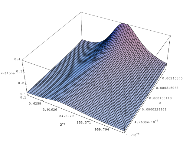
Figure 1: The $x$-slope $\frac{\partial lnF_{2}^{p}(x,Q^{2})}{\partial ln(1/x)}$ as a function of $x$ and $Q^{2}$.

Figure 2: The effective intercept measured experimentally and comparison with our model. (The asterisks denote the points where $\frac{\partial lnF_{2}^{p}(x,Q^{2})}{\partial ln(1/x)}$ was calculated.)

4.2 $Q$-SLOPE OR ${\partial F_{2}^{p}(x,Q^{2})/\partial ln(Q^{2})}$

The data on the $Q$-slope shows a peak at $Q^{2}\sim 1-5\;GeV^{2}$. This peak is interpreted as a transition from Regge behaviour to a perturbative QCD regime. We performed calculation in the framework of our model and the result is in Figure. 3. As is seen, there is no contradiction in the behaviour of the $Q$-slope and Regge regime. We also want to emphasise that the determination of the transition region depends on the path on the two-dimentional surface of ${\partial F_{2}^{p}(x,Q^{2})/\partial ln(Q^{2})}$ and it may lead to the $x$-dependence of the position of the peak $\!{}^{{\bf?}}$. To demonstrate this we show this surface calculated in our model in Figure 4.

Figure 3: The $Q$-slope $\frac{\partial F_{2}^{p}(x,Q^{2})}{\partial ln(Q^{2})}$ (The asterisks denote the points where $\frac{\partial lnF_{2}^{p}(x,Q^{2})}{\partial ln(1/x)}$ was calculated.)

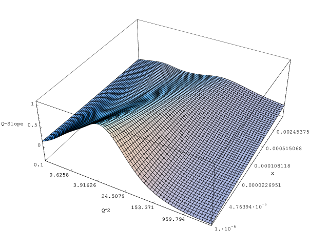
Figure 4: The $Q$-slope $\frac{\partial F_{2}^{p}(x,Q^{2})}{\partial ln(Q^{2})}$ as a function of $x$ and $Q^{2}$.

5 CONCLUSION

The proton structure function $F_{2}^{p}(x,Q^{2})$ is described in the framework of extended Regge-eikonal approach. It is argued that for this one does not need additional Regge poles with intercepts depending on $Q^{2}$. The experimental data on $x$- and $Q$-slope are also described fairly well. The model predicts damping of the HERA effect (the similar prediction is made in the framework of the Dipole pomeron model $\!{}^{{\bf?}}$).

Figure 5: Experimental data for the proton structure function $F_{2}^{p}(x,Q^{2})$ at low and intermediate $Q^{2}$ and predictions of the model.

Figure 6: Experimental data for the proton structure function $F_{2}^{p}(x,Q^{2})$ at intermediate and high $Q^{2}$ and predictions of the model.

References

- [1] K. Adel, F. Barreiro, F.J. Ynduráin, Nucl. Phys. B 495, 211 (1997) E. Martynov, in Proceedings of the workshop on soft physics “Hadron-94”, Uzhgorod, Ukraine, September 1994, edited by G.Bugrij, L.Jenkovszky, E.Martynov (Kiev 1994), p.311; in Proceedings of the VI Blois Conference on Elastic and Diffractive Scattering, Blois, France,June 1995, edited by P. Chiapetta, M. Haguenauer, J. Trân Thanh Vân (Editions Frontiéres 1996), p.203 L. Jenkovszky, E.Martynov, F. Paccanoni, Regge behaviour of nucleon structure function. PFDP 95/TH/21, Padova University (1995) W. Buchmuller, D. Haidt, Double-logarithmic Scaling of the Structure Function at small DESY 96-061; hep-ph/9605428 (1996) D. Schildknecht, H. Spiesberger Generalized Vector Dominance and low x inelastic electron-proton scattering BI-TP 97/25;hep-ph/9707447 (1997) P. Desgrolard et al., Phys. Lett. B 309, 191 (1993). P. Desgrolard, A. Lengyel, E. Martynov, New possibilities of old soft pomeron in DIS Eur.Phys.J. C 655, C7 (1999)
- [2] A. Capella et al, Phys. Lett. B 349, 561 (1995). H. Abramovicz et al, Phys. Lett. B 269, 465 (1991). Halina Abramowicz and Aharon Levy, The ALLM parameterization of - an update, DESY 97-251, hep-ph/9712415 (1997); A Donnachie, The two pomerons, in Proceedings of the summer school on hadronic aspects of collider physics, Zuoz, 1994, edited by E.P. Locher (Villigen, PSI-Proceedings, 94-01, 1994), p. 135; M. Bertini, M. Giffon, E. Predazzi, Phys. Lett. B 349, 561 (1995); A Donnachie, P V Landshoff, Small x: Two Pomerons!, Phys. Lett. B 437, 408 (1998); C. Merino, A. B. Kaidalov, D. Pertermann The CKMT Model and the Theoretical Description of the Caldwell-plot hep-ph/9911331.
- [3] V. Petrov, Proc. of the VIth Blois Workshop, Editions Frontiéres, 1995 p. 139;Nucl. Phys. B 54A, 160 (1997)(Proc. Suppl.)
-
[4]
M. Froissart, Phys. Rev. D 123, 1053 (1961)
A. Martin, Phys. Rev. D 129, 993 (1963). - [5] P. Desgrolard, A. Lengyel, E. Martynov, Eur.Phys.J. C 7, 655 (1999)
- [6] V. Petrov, A. Prokudin, “Extended Regge Eikonal Approach versus Experimental Data” ,to be published in the proceedings of the International Conference on Elastic and Diffractive Scattering, Russia, Protvino 1999
- [7] N. M. Kroll, T. D. Lee, B. Zumino Phys. Rev. D 157, 1376 (1967)