Zee Neutrino Mass Model in a SUSY Framework

Abstract

We study the Zee model of neutrino mass in the framework of $R$-parity violating supersymmetry. Within the matter contents of the minimal supersymmetric standard model, any one of the three right-handed sleptons could be a suitable candidate for the charged-singlet scalar of the Zee model, and one of the Higgs doublets provides the extra necessary vacuum expectation value. A combination of one bilinear and two trilinear $R$-parity-violating couplings then completes the model. In this framework, we also discuss other various contributions to neutrino masses and derive the conditions for the dominance of the contribution from the Zee model, and hence maintain the successfully Zee mass texture. However, this model within the minimal supersymmetric standard model is shown to be only marginally feasible. More general versions of supersymmetrization of the Zee model are also discussed. A particularly interesting example that has extra Higgs doublets while the slepton, especially the selectron, keeps the role of the Zee scalar is illustrated.

I Introduction

Within the standard model (SM), the $V-A$ nature of the weak interaction dictates a zero mass for all three families of neutrinos. The discovery of neutrino mass(es) or oscillation(s) will certainly push for new physics. Evidence for neutrino oscillations has been collected in a number of solar neutrino and atmospheric neutrino experiments. The most impressive results were the recent $\nu_{\mu}$ neutrino deficit and the asymmetric zenith-angle distribution observed by the Super-Kamiokande Collaboration [1].

The atmospheric neutrino deficit and zenith-angle distribution can be explained by the $\nu_{\mu}-\nu_{\tau}$ or $\nu_{\mu}-\nu_{s}$ oscillations ($\nu_{s}$ is a sterile neutrino that has negligible coupling to $W$ or $Z$ boson and the former has a slightly better fit). The oscillation parameters with $\nu_{\mu}\to\nu_{\tau}$ at 90% C.L. are [1]

$$\Delta m^{2}_{\rm atm}\simeq(2-6)\times 10^{-3}\;{\rm eV}^{2},\;\sin^{2}2\theta_{\rm atm}\gtrsim 0.85\;.$$

On the other hand, the solar neutrino deficit admits more than one solution. With $\nu_{e}\to\nu_{\tau}$ the solutions at 95% C.L. are [2]

vacuum oscillation: $$\Delta m^{2}_{\rm sol}\simeq(5-8)\times 10^{-11}\;{\rm eV}^{2},\;\sin^{2}2\theta_{\rm sol}\simeq 0.6-1.0\;,$$ (1)

small angle MSW: $$\Delta m^{2}_{\rm sol}\simeq(4-9)\times 10^{-6}\;{\rm eV}^{2},\;\sin^{2}2\theta_{\rm sol}\simeq(3.5-13)\times 10^{-3}\;,$$ (2)

large angle MSW: $$\Delta m^{2}_{\rm sol}\simeq(8-30)\times 10^{-6}\;{\rm eV}^{2},\;\sin^{2}2\theta_{\rm sol}\simeq 0.4-0.8\;.$$ (3)

The above two neutrino-mass differences can be accommodated by the three species of neutrinos that we know from the SM. There is also another indication for neutrino oscillation from the accelerator experiment at the Liquid Scintillation Neutrino Detector (LSND) [3], which requires an oscillation of $\nu_{\mu}$ into another neutrino with

$$\Delta m^{2}_{\rm LSND}\simeq 0.2-2\;{\rm eV}^{2}\;,\sin^{2}2\theta_{\rm LSND}\simeq 0.003-0.03\;.$$

To as well accommodate this data it requires an additional species of neutrino beyond the usual neutrinos. Nevertheless, further evidence from the next round of neutrino experiments is required to confirm the neutrino mass and oscillation. As neutrino is favored to be massive it is desirable to understand the generation of neutrino masses from physics beyond the SM, especially, to see if the new physics can give a neutrino mass pattern that can explain the atmospheric and solar neutrino data, and perhaps the LSND as well.

An economical way to generate small neutrino masses with a phenomenologically favorable texture is given by the Zee model [4, 5, 6], which generates masses via one-loop diagrams. The model consists of a charged gauge singlet scalar $h^{\mbox{-}}$, the Zee scalar, which couples to lepton doublets $\psi_{\!\scriptscriptstyle Lj}$ via the interaction

$$f^{ij}\left(\psi^{\alpha}_{\!\scriptscriptstyle Li}{\cal C}\psi^{\beta}_{\!\scriptscriptstyle Lj}\right)\epsilon_{\!\scriptscriptstyle\alpha\beta}\;h^{\scriptscriptstyle-}\;,$$ (4)

where $\alpha,\beta$ are the SU(2) indices, $i,j$ are the generation indices, ${\cal C}$ is the charge-conjugation matrix, and $f^{ij}$ are Yukawa couplings antisymmetric in $i$ and $j$. Another ingredient of the Zee model is an extra Higgs doublet (in addition to the one that gives masses to charged leptons) that develops a vacuum expectation value (VEV) and thus provides mass mixing between the charged Higgs boson and the Zee scalar boson. The corresponding coupling, together with the $f^{ij}$’s, enforces lepton number violation. The one-loop mechanism for the Zee model can be found in Fig. 1.

A recent analysis by Frampton and Glashow [5] (see also Ref.[6]) showed that the Zee mass matrix of the following texture

$$\left(\begin{array}[]{ccc}0&m_{e\mu}&m_{e\tau}\\ m_{e\mu}&0&\epsilon\\ m_{e\tau}&\epsilon&0\end{array}\right)\;,$$ (5)

where $\epsilon$ is small compared with $m_{e\mu}$ and $m_{e\tau}$, is able to provide a compatible mass pattern that explains the atmospheric and solar neutrino data. The generic Zee model guarantees the vanishing of the diagonal elements, while the suppression of the $m_{\mu\tau}$ entry, here denoted by the small parameter $\epsilon$, has to be otherwise enforced. Moreover, $m_{e\mu}\sim m_{e\tau}$ is required to give the maximal mixing solution for the atmospheric neutrinos. We shall describe the features in more detail in the next section.

So far the Zee model is not embedded into any grand unified theories or supersymmetric models. Here we analyze the embedding of the Zee model into the minimal supersymmetric standard model (MSSM) with minimal extensions, namely, the $R$-parity violation. The right-handed sleptons in SUSY have the right quantum number to play the role of the charged Zee scalar. The $R$-parity-violating $\lambda$-type couplings ($\lambda LLE$) could provide the terms in Eq.(4). It is also easy to see that the $R$-parity-violating bilinear $\mu$-type couplings ($\mu_{i}LH_{\scriptscriptstyle 2}$) would allow the second Higgs doublet $H_{\scriptscriptstyle 2}$ in SUSY to be the second ingredient of the Zee model. So far so good. However, the SUSY framework dictates extra contributions to neutrino masses, which deviate from the texture of the Zee mass matrix of Eq. (5). The major objective of this paper is to address the feasibility of the embedding and to determine under what conditions could one make a supersymmetric Zee model within the $R$-parity-violating SUSY framework while retaining the successful flavor of the former. We will also discuss briefly more generic versions of supersymmetric Zee model. There is also a study of Zee mass matrix within the framework of gauge-mediated SUSY breaking with the messenger field as the Zee singlet [7].

In $R$-parity-violating SUSY, there are three other sources for neutrino masses, in addition to the Zee model contribution. They are (i) the tree-level mixing with the higgsinos and gauginos, (ii) the one-loop diagram that involves the usual mass mixing between the left-handed and right-handed sleptons proportional to $m_{\scriptscriptstyle\ell}\,(A^{\!\scriptscriptstyle E}_{\scriptscriptstyle\ell}-\mu\tan\beta)$, and (iii) the one-loop diagram that again involves the mixing between the left-handed and right-handed sleptons but this time via the $\lambda$ and $\mu_{i}$ couplings. The first two contributions have been considered extensively in literature [9], but the last one is identified here for the first time. Also, we are the first one to identify the Zee model contribution to the neutrino mass in the SUSY framework. Furthermore, we will obtain the conditions for the Zee model contribution to dominate over the contributions in (i) and (ii). The contribution in (iii) can actually preserve the texture of the mass matrix of Eq. (5).

There are complications in choosing a flavor basis when $R$ parity is broken. Actually, the form and structure of the lepton mass matrices under the coexistence of bilinear and trilinear $R$-parity-violating couplings are basis dependent. One has to be particularly careful with a consistent choice of flavor basis. Here we adopt the single-VEV parametrization [10] that provides an efficient framework for our study. The most important point to note here is that this parametrization implies a choice of flavor basis under which all three sneutrinos have no VEV, without any input assumptions. All $R$-parity-violating couplings introduced below are to be interpreted under this basis choice.

The organization of the paper is as follows. In the next section, we describe the texture of the Zee mass matrix in Eq. (5). In Sec. III, we calculate entries in the $3\times 3$ neutrino mass matrix from all the sources listed above. In Sec. IV, we derive the conditions for the contributions from the Zee model and from (iii) above to be dominant. Section V is devoted to discussions on more general versions of supersymmetrization of the Zee model. We conclude in Sec. VI.

II Zee Mass Matrix

Here we briefly describe the basic features of the Zee mass matrix, as given in Eq.(5). We first take $\epsilon=0$. The matrix can be diagonalized by the following transformation

$$\left(\begin{array}[]{c}\nu_{\!\scriptscriptstyle Le}\\ \nu_{\!\scriptscriptstyle L\mu}\\ \nu_{\!\scriptscriptstyle L\tau}\end{array}\right)=\left(\begin{array}[]{ccc}\frac{1}{\sqrt{2}}&\frac{1}{\sqrt{2}}&0\\ \frac{m_{e\mu}}{\sqrt{2}m}&\frac{-m_{e\mu}}{\sqrt{2}m}&\frac{-m_{e\tau}}{m}\\ \frac{m_{e\tau}}{\sqrt{2}m}&\frac{-m_{e\tau}}{\sqrt{2}m}&\frac{m_{e\mu}}{m}\end{array}\right)\;\left(\begin{array}[]{c}\nu_{\!\scriptscriptstyle L_{1}}\\ \nu_{\!\scriptscriptstyle L_{2}}\\ \nu_{\!\scriptscriptstyle L_{3}}\end{array}\right)\;,$$ (6)

with the eigenvalues $m,-m,0$ for $\nu_{\!\scriptscriptstyle L_{1}},\nu_{\!\scriptscriptstyle L_{2}},\nu_{\!\scriptscriptstyle L_{3}}$, respectively, and $m=\sqrt{m_{e\mu}^{2}+m_{e\tau}^{2}}$. Hence, the two massive states form a Dirac pair. The atmospheric mass-squared difference $\Delta m^{2}_{\rm atm}\simeq 3\times 10^{-3}{\rm eV}^{2}$, is to be identified with $m^{2}=m_{e\mu}^{2}+m_{e\tau}^{2}$. The transition probabilities for $\nu_{\!\scriptscriptstyle L_{\mu}}$ are

$$P_{\nu_{\scriptscriptstyle L_{\mu}}\to\nu_{\scriptscriptstyle L_{e}}} = 0\;,$$ (7)

$$P_{\nu_{\scriptscriptstyle L_{\mu}}\to\nu_{\scriptscriptstyle L_{\tau}}} = 4\left(\frac{m_{e\mu}m_{e\tau}}{m_{e\mu}^{2}+m_{e\tau}^{2}}\right)^{2}\sin^{2}\left(\frac{(m_{e\mu}^{2}+m_{e\tau}^{2})L}{4E}\right)\;.$$ (8)

If $m_{e\mu}\simeq m_{e\tau}$, then $\sin^{2}2\theta_{\rm atm}\simeq 1$. This mixing angle is exactly what is required in the atmospheric neutrino data. The neutrino mass matrix texture with $\epsilon=0$ can be called the zeroth order Zee texture. It is the first thing to aim at in our supersymmetric model discussions in the next section.

If we choose a nonzero $\epsilon$, but keep $\epsilon\ll m_{e\mu,e\tau}$. Then after diagonalizing the matrix we have the following eigenvalues

$$m_{\nu\scriptscriptstyle 1} = \sqrt{m_{e\mu}^{2}+m_{e\tau}^{2}}+\epsilon\frac{m_{e\mu}m_{e\tau}}{m_{e\mu}^{2}+m_{e\tau}^{2}}\;,$$ (9)

$$m_{\nu\scriptscriptstyle 2} = -\sqrt{m_{e\mu}^{2}+m_{e\tau}^{2}}+\epsilon\frac{m_{e\mu}m_{e\tau}}{m_{e\mu}^{2}+m_{e\tau}^{2}}\;,$$ (10)

$$m_{\nu\scriptscriptstyle 3} = -2\epsilon\frac{m_{e\mu}m_{e\tau}}{m_{e\mu}^{2}+m_{e\tau}^{2}}\;.$$ (11)

The mass-square difference between $m^{2}_{\nu\scriptscriptstyle 1}$ and $m^{2}_{\nu\scriptscriptstyle 2}$ can be fitted to the solar neutrino mass. For instance, one can take the large angle Mikheyev-Smirnov-Wolfenstein (MSW) solution and requires

$$4\epsilon\frac{m_{e\mu}m_{e\tau}}{\sqrt{m_{e\mu}^{2}+m_{e\tau}^{2}}}=\Delta m^{2}_{\rm sol}\simeq 2\times 10^{-5}\;{\rm eV}^{2}\;,$$

giving

$$\frac{\epsilon}{m_{e\mu}}\sim 5\times 10^{-3}\;,$$

where we have used $m_{e\mu}\simeq m_{e\tau}$.

We will see below that in our supersymmetric model the couplings that are required to generate the zeroth order Zee texture also give rise to other contributions, which have to be kept subdominating in order to maintain the texture and hence the favor of the Zee model. Even though these extra contributions might not be identified as the same entries as the ${\epsilon}$ parameter of Eq. (5), i.e., appear in the diagonal entries instead, they could still play the same role as to give a phenomenologically viable first order result for a modified Zee matrix. Hence, we will not commit ourselves to the first order Zee matrix as given in Eq.(5), but only to its zeroth order form, namely with ${\epsilon}=0$. The first order perturbation is then allowed to come in through any matrix entry. It will split the mass square degeneracy of the Dirac pair similar to the ${\epsilon}$ case above. For example, if the first order perturbation is given by a $\epsilon_{\scriptscriptstyle d}$ appearing at the $m_{ee}$ entry, the resulting mass eigenvalues are modified to

$$m_{\nu\scriptscriptstyle 1} = \sqrt{m_{e\mu}^{2}+m_{e\tau}^{2}}+\frac{\epsilon_{\scriptscriptstyle d}}{2}\;,$$ (12)

$$m_{\nu\scriptscriptstyle 2} = -\sqrt{m_{e\mu}^{2}+m_{e\tau}^{2}}+\frac{\epsilon_{\scriptscriptstyle d}}{2}\;,$$ (13)

$$m_{\nu\scriptscriptstyle 3} = 0\;.$$ (14)

The mass-square difference between $m^{2}_{\nu\scriptscriptstyle 1}$ and $m^{2}_{\nu\scriptscriptstyle 2}$ can then be fitted to the solar neutrino data and we obtain $\epsilon_{\scriptscriptstyle d}/m_{e\mu}\sim 5\times 10^{-3}$, the same as above. If, on the other hand, $\epsilon_{\scriptscriptstyle d}$ appears at the $m_{\mu\mu}$ or $m_{\tau\tau}$ entry, the solar neutrino data can still be fitted and $\epsilon_{\scriptscriptstyle d}/m_{e\mu}\sim 1\times 10^{-2}$ is required. Once the zeroth order Zee texture for the atmospheric neutrino is satisfied, it is straightforward to further impose the above condition for the solar neutrino.

III Neutrino Mass Matrix

First consider the superpotential as given by

$$W=\epsilon_{\!\scriptscriptstyle\alpha\beta}\Biggr{\{}Y_{ij}^{\!\scriptscriptstyle U}Q^{\alpha}_{i}H_{\!\scriptscriptstyle 2}^{\beta}U_{j}^{c}+Y_{ij}^{\!\scriptscriptstyle D}Q_{i}^{\alpha}H_{\!\scriptscriptstyle 1}^{\beta}D^{c}_{j}+Y^{\!\scriptscriptstyle E}_{ij}L_{i}^{\alpha}H_{\!\scriptscriptstyle 1}^{\beta}E^{c}_{j}\\ +\mu H_{\!\scriptscriptstyle 1}^{\alpha}H_{\!\scriptscriptstyle 2}^{\beta}+\lambda_{ijk}L_{i}^{\alpha}L_{j}^{\beta}E^{c}_{k}+\mu_{i}L_{i}^{\alpha}H_{\!\scriptscriptstyle 2}^{\beta}\Biggr{\}}\;,$$ (15)

where $\epsilon_{\scriptscriptstyle 12}=-\epsilon_{\scriptscriptstyle 21}=-1$, $i,j=1,2,3$ are the generation indices. $H_{\scriptscriptstyle 1}=(h^{0}_{\scriptscriptstyle 1},h^{\mbox{-}}_{\scriptscriptstyle 1}),H_{\scriptscriptstyle 2}=(h^{+}_{\scriptscriptstyle 2},h^{0}_{\scriptscriptstyle 2})$. In the above equation, $Q,L,U^{c},D^{c},E^{c},H_{\scriptscriptstyle 1}$, and $H_{\!\scriptscriptstyle 2}$ denote the quark doublet, lepton doublet, up-quark singlet, down-quark singlet, lepton singlet, and the two Higgs doublet superfields. Here we allow only the $R$-parity violation through the terms $LLE^{c}$ and $LH_{\!\scriptscriptstyle 2}$ with coefficients $\lambda_{ijk}$ (antisymmetric in $i,j$) and $\mu_{i}$, respectively. The other $R$-parity-violating couplings are dropped as they are certainly beyond the minimal framework needed for embedding the Zee model. The soft SUSY breaking terms that are relevant to our study are

$\displaystyle(Y^{\!\scriptscriptstyle E}\!A^{\!\scriptscriptstyle E})_{ij}\tilde{L}^{\alpha}_{i}H_{\!\scriptscriptstyle 1}^{\beta}\tilde{E}^{c}_{j}+(\lambda A^{\!\lambda})_{ijk}\tilde{L}^{\alpha}_{i}\tilde{L}^{\beta}_{j}\tilde{E}^{c}_{k}+\mu BH_{\!\scriptscriptstyle 1}^{\alpha}H_{\!\scriptscriptstyle 2}^{\beta}\;.$

Actually, the $(\lambda A^{\!\lambda})$ terms do not contribute because our choice of basis eliminates the VEV’s for $\tilde{L}_{i}$’s. This simplifies the analysis without lose of generality. We adopt the single-VEV parametrization, which uses the $L_{i}$ basis such that the charged-lepton Yukawa matrix $Y^{\!\scriptscriptstyle E}$ is diagonal. The whole $(Y^{\!\scriptscriptstyle E}\!A^{\!\scriptscriptstyle E})$ term will be taken as predominantly diagonal, namely, $(Y^{\!\scriptscriptstyle E}\!A^{\!\scriptscriptstyle E})_{ij}\approx Y^{\!\scriptscriptstyle E}_{i}A^{\!\scriptscriptstyle E}_{i}\delta_{ij}\,\mbox{(no sum)}$. This is just the common practice of suppressing off-diagonal $A$ terms, favored by flavor-changing neutral-current constraints.

The tree-level mixing among the higgsinos, gauginos, and neutrinos gives rise to a $7\times 7$ neutral fermion mass matrix $\cal{M_{N}}$:

$$\cal{M_{N}}=\left(\begin{array}[]{cccc|ccc}M_{\scriptscriptstyle 1}&0&g^{\prime}v_{\scriptscriptstyle 2}/2&-g^{\prime}v_{\scriptscriptstyle 1}/2&0&0&0\\ 0&M_{\scriptscriptstyle 2}&-gv_{\scriptscriptstyle 2}/2&gv_{\scriptscriptstyle 1}/2&0&0&0\\ g^{\prime}v_{\scriptscriptstyle 2}/2&-gv_{\scriptscriptstyle 2}/2&0&-\mu&-\mu_{\scriptscriptstyle 1}&-\mu_{\scriptscriptstyle 2}&-\mu_{\scriptscriptstyle 3}\\ -g^{\prime}v_{\scriptscriptstyle 1}/2&gv_{\scriptscriptstyle 1}/2&-\mu&0&0&0&0\\ \hline\cr 0&0&-\mu_{1}&0&(m_{\nu}^{0})_{\!\scriptscriptstyle 1\!1}&(m_{\nu}^{0})_{\!\scriptscriptstyle 1\!2}&(m_{\nu}^{0})_{\!\scriptscriptstyle 1\!3}\\ 0&0&-\mu_{\!\scriptscriptstyle 2}&0&(m_{\nu}^{0})_{\!\scriptscriptstyle 2\!1}&(m_{\nu}^{0})_{\!\scriptscriptstyle 22}&(m_{\nu}^{0})_{\!\scriptscriptstyle 23}\\ 0&0&-\mu_{\!\scriptscriptstyle 3}&0&(m_{\nu}^{0})_{\!\scriptscriptstyle 31}&(m_{\nu}^{0})_{\!\scriptscriptstyle 32}&(m_{\nu}^{0})_{\!\scriptscriptstyle 33}\\ \end{array}\right)\;,$$ (16)

whose basis is $(-i\tilde{B},-i\tilde{W},\tilde{h}_{\scriptscriptstyle 2}^{0},\tilde{h}_{\scriptscriptstyle 1}^{0},\nu_{\!\scriptscriptstyle L_{e}},\nu_{\!\scriptscriptstyle L_{\mu}},\nu_{\!\scriptscriptstyle L_{\tau}})$. Each of the charged-lepton states deviates from its physical state as a result of its mixing with higgsino-gaugino through the corresponding $\mu_{i}$ term[10]. However, we are interested only in a region of the parameter space where the concerned deviations are negligible, as also discussed in Ref.[11]. Hence, we are effectively in the basis of the physical charged-lepton states, as indicated. In the above $7\times 7$ matrix, the whole lower-right $3\times 3$ block $(m_{\nu}^{0})$ is zero at tree level. They are induced via one-loop contributions to be discussed below. One-loop contributions to the other zero entries are neglected. We can write the mass matrix in the form of block submatrices:

$${\cal M_{N}}=\left(\begin{array}[]{c|c}{\cal M}&\xi^{\!\scriptscriptstyle T}\\ \hline\cr\xi&m_{\nu}^{0}\end{array}\right)\;,$$ (17)

where $\cal{M}$ is the upper-left $4\times 4$ neutralino mass matrix, $\xi$ is the $3\times 4$ block, and $m_{\nu}^{0}$ is the lower-right $3\times 3$ neutrino block in the $7\times 7$ matrix. The resulting neutrino mass matrix after block diagonalization is given by

$$(m_{\nu})=-\xi{\cal M}^{\mbox{-}1}\xi^{\!\scriptscriptstyle T}+(m_{\nu}^{0})\;.$$ (18)

The first term here corresponds to tree level contributions, which are, however, see-saw suppressed.

Before going into our best scenario analysis, we will sketch how the couplings, $\lambda_{ijk}$’s and $\mu_{i}$’s, lead to the neutrino mass terms. While some of them have been studied in literature, others are identified here for the first time. We do this from the perspectives of the supersymmetric Zee model, but the results are quite general.

Our minimalistic strategy says that a $\lambda_{ijk}$ or a $\mu_{i}$ should be taken as zero unless it is needed for the Zee mechanism to generate the neutrino mass terms $m_{e\mu}$ and $m_{e\tau}$. Readers who find the extensive use of unspecified indices in the following discussions difficult to follow are suggested to match them with the results for the explicit examples that we will list below. We identify the following four neutrino-mass generation mechanisms.

(i) Zee mechanism. We show in Fig. 1, the two Zee diagrams for the one-loop neutrino mass terms. The right-handed slepton $\tilde{\ell}_{\!\scriptscriptstyle R_{k}}$ is identified as the charged-singlet boson of the Zee model, and its coupling to lepton fields has the correct antisymmetric generation indices: see Eq. (4). To complete the diagram the charged Higgs boson $h_{\scriptscriptstyle 1}^{\mbox{-}}$ from the Higgs doublet $H_{\scriptscriptstyle 1}$ is on the other side of the loop and a $\tilde{\ell}_{\!\scriptscriptstyle R_{k}}$-$h_{1}^{\mbox{-}}$ mixing is needed at the top of the loop. Such a mixing is provided by a $F$ term of $L_{k}$: $\mu_{k}m_{\!\scriptscriptstyle\ell_{k}}h_{\scriptscriptstyle 1}^{\mbox{-}}\tilde{\ell}^{*}_{\!\scriptscriptstyle R_{k}}\langle h_{\scriptscriptstyle 2}^{0}\rangle/\langle h_{\scriptscriptstyle 1}^{0}\rangle$, where $h_{\scriptscriptstyle 2}^{0}$ takes on its VEV, for a nonzero $\mu_{k}$. Thus, the neutrino mass term $(m_{\nu}^{0})_{ij}$ has a

$$\mu_{k}m_{\!\scriptscriptstyle\ell_{k}}\lambda_{ijk}(m_{\!\scriptscriptstyle\ell_{j}}^{2}-m_{\!\scriptscriptstyle\ell_{i}}^{2})$$ (19)

dependence, where $m_{\!\scriptscriptstyle\ell_{i}}$’s are the charged lepton masses.

(ii) $LR$ slepton mass mixing. Another, well-studied, type of contributions comes from the one-loop diagram with two $\lambda$-coupling vertices and the usual $(A^{\!\scriptscriptstyle E}-\mu\tan\beta)$-type $LR$ slepton mixing. Neglecting the off-diagonal entries in $A^{\!\scriptscriptstyle E}$, the contribution to $(m_{\nu}^{0})_{ij}$ with the pair $\lambda_{ilk}$ and $\lambda_{jkl}$ is proportional to

$$\big{[}\;(A^{\!\scriptscriptstyle E}_{k}-\mu\tan\!{\beta})+(1-\delta_{kl})(A^{\!\scriptscriptstyle E}_{l}-\mu\tan\!{\beta})\;\big{]}\;m_{\!\scriptscriptstyle\ell_{k}}m_{\!\scriptscriptstyle\ell_{l}}\lambda_{ilk}\lambda_{jkl}\;.$$ (20)

Only $\lambda_{ijk}$’s with all distinct indices (e.g. $\lambda_{\scriptscriptstyle 1\!23}$) fail to give contributions of this kind on its own. A nonzero $\lambda_{ikk}$ contributes to the diagonal $(m_{\nu}^{0})_{ii}$. An illustration for the term is given in Fig. 2. With any two nonzero $\lambda_{ijk}$’s, this kind of contributions to the $(m_{\nu}^{0})$ entries, in particular the diagonal ones, cannot be avoided.

(iii) $LR$ slepton mass mixing via $R$-parity violating couplings. This contribution is identified here for the first time. While the contributions to generation mixing in the usual $(A^{\!\scriptscriptstyle E}-\mu\tan\beta)$-type $LR$ slepton mixing via the off-diagonal entries in $A^{\!\scriptscriptstyle E}$ are expected to be small, there is another independent source of generation mixing in the $LR$ slepton-mass mixing, which may not follow the rule. The latter comes from a $F$ term of $L_{i}$: $\mu_{i}\lambda_{ijk}\tilde{\ell}_{\!\scriptscriptstyle L_{j}}\tilde{\ell}^{*}_{\!\scriptscriptstyle R_{k}}\langle h_{\scriptscriptstyle 2}^{0}\rangle$, where $h_{\scriptscriptstyle 2}^{0}$ takes on the VEV. This is similar to the $\tilde{\ell}_{\!\scriptscriptstyle R_{k}}\!\mbox{-}h_{\scriptscriptstyle 1}^{\mbox{-}}$ mixing in the Zee model, except that this time we have a $\lambda$-type coupling instead of the $R$-parity-conserving Yukawa coupling. This newly identified source of mixing results in constraints on the $\mu_{i}\lambda_{ijk}$ products, which is an interesting subject of lepton-slepton phenomenology studies.

With a specific choice of a set of nonzero $\mu_{i}$’s and $\lambda$’s, this type of mixing gives rise to the off-diagonal $(m_{\nu}^{0})_{ij}$ terms only and, therefore, of particular interest to our perspectives of Zee model. Taking the pair $\lambda_{ilk}$ and $\lambda_{jhl}$ for the fermion vertices and a $F$ term of $L_{g}$ providing a coupling for the scalar vertex in the presence of a $\mu_{g}$ and a $\lambda_{ghk}$ (see Fig. 3), a $(m_{\nu}^{0})_{ij}$ term is generated and proportional to

$$\mu_{g}m_{\!\scriptscriptstyle\ell_{l}}\lambda_{ghk}\lambda_{ilk}\lambda_{jhl}\;.$$ (21)

The proliferation of indices here is certainly difficult to keep track of. When we allow only a single nonzero $\lambda$ at a time, the only contribution comes from $\lambda_{ijj}$ but not from those with distinct indices. Suppose we have nonzero $\lambda_{ijj}$ and $\mu_{j}$, they then give a contribution to the off-diagonal $(m_{\nu}^{0})_{ij}$ with a

$\displaystyle\mu_{j}m_{\!\scriptscriptstyle\ell_{j}}\lambda_{ijj}^{3}$

dependence, which is obtained from expression (21) through the substitution $h=i$ and $g=k=l=j$. It is easy to see that for a minimal set of nonzero $\mu_{i}$ and $\lambda_{ijk}$ required to generate the zeroth order Zee texture, this minimal set also contributes to the same neutrino mass terms via the new mechanism identified here. Hence, they are desirable from the perspectives of keeping the Zee mass matrix texture.

(iv) Tree-level mixing. Through gaugino-higgsino mixings, nonzero $\mu_{i}$’s give tree-level see-saw type contributions to $(m_{\nu})_{ij}$ proportional to $\mu_{i}\mu_{j}$, i.e., through the first term in Eq.(18) instead of the second. With the contribution put in explicitly, Eq.(18) then gives

$$(m_{\nu})_{ij}=-\,\frac{v^{2}\cos^{2}\!\beta\;(g^{2}M_{\scriptscriptstyle 1}+g^{{}^{\prime}2}M_{\scriptscriptstyle 2})}{2\mu\;[2\mu M_{\scriptscriptstyle 1}M_{\scriptscriptstyle 2}-v^{2}\sin\!\beta\cos\!\beta\;(g^{2}M_{\scriptscriptstyle 1}+g^{{}^{\prime}2}M_{\scriptscriptstyle 2})]}\;\mu_{i}\mu_{j}+(m_{\nu}^{0})_{ij}\;.$$ (22)

A diagonal $(m_{\nu})_{kk}$ term is always present for a nonzero $\mu_{k}$ as needed in the Zee mechanism. This contribution has no charged lepton mass dependence. To eliminate these tree-level terms requires either very stringent constraints on the parameter space or extra Higgs superfields beyond the MSSM spectrum. We will see that this is a major difficulty of the present MSSM formulation of supersymmetric Zee model.

From the above discussions, we conclude that a minimal set of $R$-parity violating couplings needed to give the zeroth order Zee matrix is the following :

$\displaystyle\{\quad\lambda_{{\scriptscriptstyle 12}\,k}\;,\quad\lambda_{{\scriptscriptstyle 13}\,k}\;,\quad\mu_{k}\quad\}\;.$

As at least one of the two $\lambda$’s has the form $\lambda_{ikk}$ ($\equiv-\lambda_{kik}$), all types of contributions that have been discussed above are there. We want to make the contribution from the Zee mechanism dominate over other contributions, or at least to make the diagonal mass entries to $(m_{\nu})$ subdominant. This necessarily requires subdomination of the contributions from the tree-level see-saw mechanism and from the $(A^{\!\scriptscriptstyle E}-\mu\tan\!{\beta})$-type $LR$ slepton mixing. So, it is the Zee mechanism and the newly identified mechanism, which involve the interplay between the bilinear $\mu_{i}$ and trilinear $\lambda_{ijk}$ $R$-parity-violating couplings, that are required to be the dominating ones.

We will discuss below two illustrative scenarios (1) $\lambda_{\scriptscriptstyle 1\!2\!1}$, $\lambda_{\scriptscriptstyle 1\!3\!1}$, and $\mu_{\scriptscriptstyle 1}$ and (2) $\lambda_{\scriptscriptstyle 1\!23}$, $\lambda_{\scriptscriptstyle 1\!33}$, and $\mu_{\scriptscriptstyle 3}$. After the $7\times 7$ matrix ${\cal M}_{\cal N}$ is block diagonalized, the resulting $3\times 3$ neutrino mass matrix $(m_{\nu})$ of Eqs.(18) or (22) is obtained in each of these scenarios.

Scenario 1: $\lambda_{\scriptscriptstyle 1\!2\!1}$, $\lambda_{\scriptscriptstyle 1\!3\!1}$, and $\mu_{\scriptscriptstyle 1}$. The resulting neutrino mass matrix for scenario 1 is given by

$$(m_{\nu})=\left(\begin{array}[]{ccc}C_{\scriptscriptstyle 1}\,\mu_{\scriptscriptstyle 1}^{2}&\;\;C_{\scriptscriptstyle 2}\,m_{e}\,m_{\mu}^{2}\,\mu_{\scriptscriptstyle 1}\lambda_{\scriptscriptstyle 1\!2\!1}+C_{\scriptscriptstyle 3}\,m_{e}\,\mu_{\scriptscriptstyle 1}\lambda_{\scriptscriptstyle 1\!2\!1}&\;\;C_{\scriptscriptstyle 2}\,m_{e}\,m_{\tau}^{2}\,\mu_{\scriptscriptstyle 1}\lambda_{\scriptscriptstyle 1\!3\!1}+C_{\scriptscriptstyle 3}\,m_{e}\,\mu_{\scriptscriptstyle 1}\lambda_{\scriptscriptstyle 1\!3\!1}\\ &C_{\scriptscriptstyle 4}\,m_{e}^{2}\,\lambda_{\scriptscriptstyle 1\!2\!1}^{2}&2C_{\scriptscriptstyle 4}\,m_{e}^{2}\,\lambda_{\scriptscriptstyle 1\!2\!1}\lambda_{\scriptscriptstyle 1\!3\!1}\\ &&C_{\scriptscriptstyle 4}\,m_{e}^{2}\,\lambda_{\scriptscriptstyle 1\!3\!1}^{2}\end{array}\right)\;,$$ (23)

which is symmetric and we only write down the upper triangle. The $C_{i}$’s are given by

$$C_{\scriptscriptstyle 1} = -\,\frac{v^{2}\cos^{2}\!\beta\;(g^{2}M_{\scriptscriptstyle 1}+g^{{}^{\prime}2}M_{\scriptscriptstyle 2})}{2\mu\;[2\mu M_{\scriptscriptstyle 1}M_{\scriptscriptstyle 2}-v^{2}\sin\!\beta\cos\!\beta\;(g^{2}M_{\scriptscriptstyle 1}+g^{{}^{\prime}2}M_{\scriptscriptstyle 2})]}\;,$$ (24)

$$C_{\scriptscriptstyle 2} = \frac{-1}{16\pi^{2}}\frac{\sqrt{2}\tan\!\beta}{v\cos\!\beta}\;f(M_{h_{\scriptscriptstyle 1}^{\mbox{-}}}^{2},M_{\tilde{e}_{R}}^{2})\;,$$ (25)

$$C_{\scriptscriptstyle 3} = \frac{1}{16\pi^{2}}\frac{v\sin\!\beta}{\sqrt{2}}\left[\lambda_{\scriptscriptstyle 1\!2\!1}^{2}\;f(M_{\tilde{\mu}_{L}}^{2},M_{\tilde{e}_{R}}^{2})+\lambda_{\scriptscriptstyle 1\!3\!1}^{2}\;f(M_{\tilde{\tau}_{L}}^{2},M_{\tilde{e}_{R}}^{2})\right]\;,$$ (26)

$$C_{\scriptscriptstyle 4} = -\frac{1}{16\pi^{2}}\;(A^{\!\scriptscriptstyle E}_{e}-\mu\tan\!\beta)\;f(M^{2}_{\tilde{e}_{L}},M^{2}_{\tilde{e}_{R}})\;,$$ (27)

where

$\displaystyle f(x,y)=\frac{1}{x-y}\;\log\left(\frac{y}{x}\right)\;.$

Scenario 2: $\lambda_{\scriptscriptstyle 1\!23}$, $\lambda_{\scriptscriptstyle 1\!33}$, and $\mu_{\scriptscriptstyle 3}$. For scenario 2, the neutrino mass matrix is given by

$$(m_{\nu})=\left(\begin{array}[]{ccc}C^{\prime}_{\scriptscriptstyle 4}\,m_{\tau}^{2}\,\lambda_{\scriptscriptstyle 1\!33}^{2}&\;\;C^{\prime}_{\scriptscriptstyle 2}\,m_{\tau}\,m_{\mu}^{2}\,\mu_{\scriptscriptstyle 3}\lambda_{\scriptscriptstyle 1\!23}+C_{\scriptscriptstyle 5}\;m_{\tau}\,\mu_{\scriptscriptstyle 3}\lambda_{\scriptscriptstyle 1\!23}\lambda_{\scriptscriptstyle 1\!33}^{2}&\;\;C^{\prime}_{\scriptscriptstyle 2}\,m_{\tau}^{3}\,\mu_{\scriptscriptstyle 3}\lambda_{\scriptscriptstyle 1\!33}+C_{\scriptscriptstyle 5}\;m_{\tau}\,\mu_{\scriptscriptstyle 3}\lambda_{\scriptscriptstyle 1\!33}^{3}\\ &0&0\\ &&C_{\scriptscriptstyle 1}\;\mu_{\scriptscriptstyle 3}^{2}\end{array}\right)\;,$$ (28)

where

$$C^{\prime}_{\scriptscriptstyle 4} = -\frac{1}{16\pi^{2}}\;(A^{\!\scriptscriptstyle E}_{\tau}-\mu\tan\!\beta)\;f(M^{2}_{\tilde{\tau}_{L}},M^{2}_{\tilde{\tau}_{R}})\;,$$ (29)

$$C^{\prime}_{\scriptscriptstyle 2} = \frac{-1}{16\pi^{2}}\frac{\sqrt{2}\tan\!\beta}{v\cos\!\beta}\;f(M_{h_{\scriptscriptstyle 1}^{\mbox{-}}}^{2},M_{\tilde{\tau}_{R}}^{2})\;,$$ (30)

$$C_{\scriptscriptstyle 5} = -\frac{1}{16\pi^{2}}\frac{v\sin\!\beta}{\sqrt{2}}f(M_{\tilde{e}_{L}}^{2},M_{\tilde{\tau}_{R}}^{2})\;.$$ (31)

In the above, we have neglected terms suppressed by $m_{e}/m_{\mu}$ or $m_{e}/m_{\tau}$. There is also another scenario, with {$\lambda_{\scriptscriptstyle 1\!22},\lambda_{\scriptscriptstyle 1\!32},\mu_{\scriptscriptstyle 2}$}, which is very similar to this scenario 2.

IV conditions for maintaining the Zee mass texture

In order to maintain the zeroth order Zee texture as discussed in Sec. II, we need $m_{e\mu}$ and $m_{e\tau}$ to dominate over the other entries. Moreover, we need $m_{e\mu}\sim m_{e\tau}\sim\sqrt{\Delta M^{2}_{\rm atm}}(\sim 5\times 10^{-11}\;\mbox{GeV})$. Here we give an estimate of the required conditions on the model parameters, for a chosen minimal set of $R$-parity-violating couplings {$\lambda_{{\scriptscriptstyle 12}k},\lambda_{{\scriptscriptstyle 13}k,}\;\mu_{k}$; (with a specific $k$)}. Since we are interested only in the absolute value of each term and so we will drop negative signs wherever feasible. We will look at each matrix entry in Eqs. (23) and (28) carefully.

Scenario 1. Requiring the tree-level gaugino-higgsino mixing contribution to $m_{ee}$ in Eq. (23) to be negligible compared to $m_{e\mu}$, it gives

$${\mu_{\scriptscriptstyle 1}^{2}}\,\cos^{2}\!\!\beta\ll{\mu^{2}}M_{\scriptscriptstyle 1}\,(1\times 10^{-14}\,{\rm GeV}^{-1})\;,$$ (32)

in which we have assumed $M_{\scriptscriptstyle 1}\approx 0.5M_{\scriptscriptstyle 2}$. The condition is rather stringent that requires either very small $\mu_{\scriptscriptstyle 1}$, $\mu_{\scriptscriptstyle 1}\cos\!\beta\ll 10^{-4}\,\mbox{GeV}$ at $M_{\scriptscriptstyle 1},\mu\sim O(100)\,\mbox{GeV}$, or particularly large gaugino mass(es). As pointed out in Ref.[10], the dependence on $\tan\!\beta$ is very important here. The $\cos\!\beta$ goes from order one to $\sim 0.02$ in the domain of large $\tan\!\beta$.

Requiring the $(A^{\!\scriptscriptstyle E}_{k}-\mu\tan\!\beta)$ $LR$ slepton mixing contribution to be much smaller than $m_{e\mu}$, we have

$$\lambda_{\scriptscriptstyle 1\!2\!1}^{2},\lambda_{\scriptscriptstyle 1\!3\!1}^{2}\ll\frac{\mbox{max}(M^{2}_{\tilde{e}_{L}},M^{2}_{\tilde{e}_{R}})}{(A^{\scriptscriptstyle E}_{e}-\mu\tan\!\beta)}\;(3\times 10^{-2}\,\mbox{GeV}^{-1})\;,$$ (33)

where we have used

$$\left[f(M^{2}_{\tilde{e}_{L}},M^{2}_{\tilde{e}_{R}})\right]^{-1}\sim\;\mbox{max}(M^{2}_{\tilde{e}_{L}},M^{2}_{\tilde{e}_{R}})\;.$$ (34)

The constraint in Eq. (33) is obviously very weak. In fact, it can certainly be neglected, especially when other phenomenological constraints [6, 12] on $\lambda$’s [as effective Zee couplings $f_{ij}$ of Eq. (4)] are taken into consideration. The relevant constraint here is given as

$$\frac{\lambda_{\scriptscriptstyle 1\!2\!1}^{2}}{M^{2}_{\tilde{e}_{R}}}\leq 10^{-8}\,\mbox{GeV}^{-2}\;,$$ (35)

from the tree-level Zee-scalar mediated $\mu$ decay [13]. The upper bound on $\lambda_{\scriptscriptstyle 1\!2\!1}$ is hence no better than $0.01$ for $M_{\tilde{e}_{R}}$ at $100\,\mbox{GeV}$. The corresponding constraint on $\lambda_{\scriptscriptstyle 1\!3\!1}$ from $\tau$ decay is definitely weaker, which has no relevance here as we will see below. Hence, the suppression needed for $m_{\mu\mu}$, $m_{\mu\tau}$, and $m_{\tau\tau}$ of Eq. (23) is easy to obtain.

The remaining question is if one can still generate the right (order of) $m_{e\mu}$ and $m_{e\tau}$ when $\mu_{\scriptscriptstyle 1}$, $\lambda_{\scriptscriptstyle 1\!2\!1}$ and $\lambda_{\scriptscriptstyle 1\!3\!1}$ satisfy the above constraints. Let us first look at the $m_{e\mu}$ entry. From Eq.(23), $m_{e\mu}$ has two contributions. The first one (the one with a $C_{\scriptscriptstyle 2}$ dependence) is from the authentic Zee mechanism. For this contribution to give the right $m_{e\mu}$ value, it requires

$$m_{e\mu}\;\sim\;\frac{\mu_{\scriptscriptstyle 1}\lambda_{\scriptscriptstyle 1\!2\!1}}{\cos^{2}\!\!\beta}\;\frac{1}{\mbox{max}(M_{h_{\scriptscriptstyle 1}^{\mbox{-}}}^{2},M_{\tilde{e}_{R}}^{2})}\;(2\times 10^{-10}\,\mbox{GeV}^{2})\;\sim\;(5\times 10^{-11}\,{\rm GeV})\;,$$ (36)

or

$$(\mu_{\scriptscriptstyle 1}\cos\!\beta)\;\lambda_{\scriptscriptstyle 1\!2\!1}\sim\;{\cos^{3}\!\!\beta}\;{\mbox{max}(M_{h_{\scriptscriptstyle 1}^{\mbox{-}}}^{2},M_{\tilde{e}_{R}}^{2})}\;(0.25\,\mbox{GeV}^{-1})\;.$$ (37)

The right-hand side above cannot be much smaller than $0.01\,\mbox{GeV}$, even at the more favorable case of very large $\tan\!\beta$. Given the above constraints in Eqs. (32) and (35), this is obviously unrealistic. Even though the corresponding contribution (with a $C_{2}$ dependence) to $m_{e\tau}$ has a $m_{\tau}^{2}/m_{\mu}^{2}$ enhancement and depends on $\lambda_{\scriptscriptstyle 1\!3\!1}$ instead of $\lambda_{\scriptscriptstyle 1\!2\!1}$, it is not much better than $m_{e\mu}$.

For the second contribution (the one with a $C_{\scriptscriptstyle 3}$ dependence), to give the right $m_{e\mu}$ value, it requires

$$m_{e\mu}\;\sim\;\mu_{\scriptscriptstyle 1}\left[\frac{\lambda_{\scriptscriptstyle 1\!2\!1}^{3}}{\mbox{max}(M_{\tilde{\mu}_{L}}^{2},M_{\tilde{e}_{R}}^{2})}+\frac{\lambda_{\scriptscriptstyle 1\!3\!1}^{2}\lambda_{\scriptscriptstyle 1\!2\!1}}{\mbox{max}(M_{\tilde{\tau}_{L}}^{2},M_{\tilde{e}_{R}}^{2})}\right](5\times 10^{-4}\,\mbox{GeV}^{2})\;\sim\;(5\times 10^{-11}\,{\rm GeV})\;.$$ (38)

A naive comparison with Eq. (36) above illustrates one important fact. Assuming a common scale for the scalar masses, the $\lambda$ coupling(s) only have to be larger than $10^{-3}$ for this second contribution to be larger than the first one. From Eqs. (33) and (35), such $\lambda$’s are easily admissible. With $\lambda_{\scriptscriptstyle 1\!2\!1}\approx\lambda_{\scriptscriptstyle 1\!3\!1}$ the corresponding contribution to $m_{e\tau}$ has the same form as $m_{e\mu}$, with the interchange of $\lambda_{\scriptscriptstyle 1\!2\!1}$ with $\lambda_{\scriptscriptstyle 1\!3\!1}$, and thus is of a similar value. The condition in Eq. (38) then becomes

$$(\mu_{\scriptscriptstyle 1}\cos\!\beta)\;\lambda_{{\scriptscriptstyle 1}i{\scriptscriptstyle 1}}\;\left(\frac{\lambda_{{\scriptscriptstyle 1}i{\scriptscriptstyle 1}}^{2}}{M_{\tilde{e}_{R}}^{2}}\right)\;\;\sim\;\cos\!\beta\;(5\times 10^{-8}\,{\rm GeV}^{-1})\;,$$ (39)

where we have taken $M_{\tilde{e}_{R}}$ to be the dominating mass among the scalars. The latter choice corresponds to the optimal case because smaller scalar masses help reducing the size of the $\lambda_{1i1}$ needed, while on the other hand, in Eq. (35) larger $M_{\tilde{e}_{R}}$ relaxes the constraint on $\lambda_{{\scriptscriptstyle 1}i{\scriptscriptstyle 1}}^{2}$. With Eqs. (32) and (35) taken into consideration, the result ends up actually no better than the best (large $\tan\!\beta$) case of Eq.(36) above.

Scenario 2. Here we follow our above analysis for this more interesting scenario. Requiring the tree-level gaugino-higgsino mixing contribution to be well below $m_{e\mu}$ gives

$${\mu_{\scriptscriptstyle 3}^{2}}\,\cos^{2}\!\!\beta\ll{\mu^{2}}M_{\scriptscriptstyle 1}\,(1\times 10^{-14}\,{\rm GeV}^{-1})\;.$$ (40)

This is basically the same as in scenario 1, though it corresponds to $m_{\tau\tau}$ instead.

For the $(A^{\scriptscriptstyle E}_{k}-\mu\tan\!\beta)$ $LR$ slepton mixing contribution to be much smaller than $m_{e\mu}$, we have

$$\lambda_{\scriptscriptstyle 1\!33}^{2}\ll\frac{\mbox{Max}(M^{2}_{\tilde{\tau}_{L}},M^{2}_{\tilde{\tau}_{R}})}{(A^{\scriptscriptstyle E}_{\tau}-\mu\tan\!\beta)}\;(2.5\times 10^{-9}\,\mbox{GeV}^{-1})\;.$$ (41)

This corresponds to $m_{ee}$. It tells us that $\lambda_{\scriptscriptstyle 1\!33}$ can hardly be much larger than $10^{-3}$. On the other hand, $\lambda_{\scriptscriptstyle 1\!23}$ is constrained differently because it does not contribute to this type of neutrino mass term. The constraint that corresponds to Eq.(35), however, becomes

$$\frac{\lambda_{\scriptscriptstyle 1\!23}^{2}}{M^{2}_{\tilde{\tau}_{R}}}\leq 10^{-8}\,\mbox{GeV}^{-2}\;,$$ (42)

which tells us that $\lambda_{\scriptscriptstyle 1\!23}$ can be as large as order of $0.01$ for scalar masses of order of $O(100)$ GeV.

Again both $m_{e\mu}$ and $m_{e\tau}$ have two terms. Let us look at $m_{e\mu}$ first. For the first term in $m_{e\mu}$ (the one with a $C^{\prime}_{\scriptscriptstyle 2}$ dependence) in Eq. (28) to give the required value of atmospheric neutrino mass, we need

$$m_{e\mu}\;\sim\;\frac{\mu_{\scriptscriptstyle 3}\lambda_{\scriptscriptstyle 1\!23}}{\cos^{2}\!\!\beta}\;\frac{1}{\mbox{max}(M_{h_{\scriptscriptstyle 1}^{\mbox{-}}}^{2},M_{\tilde{\tau}_{R}}^{2})}\;(7\times 10^{-7}\,\mbox{GeV}^{2})\;\sim\;(5\times 10^{-11}\,{\rm GeV})$$ (43)

or

$$(\mu_{\scriptscriptstyle 3}\cos\!\beta)\;\lambda_{\scriptscriptstyle 1\!23}\sim\;{\cos^{3}\!\!\beta}\;{\mbox{max}(M_{h_{\scriptscriptstyle 1}^{\mbox{-}}}^{2},M_{\tilde{\tau}_{R}}^{2})}\;(7\times 10^{-5}\,\mbox{GeV}^{-1})\;.$$ (44)

This result looks relatively promising. If we take $\cos\!\beta=0.02$, all the involved scalar masses at $100\,\mbox{GeV}$ and $\lambda_{\scriptscriptstyle 1\!23}$ at the corresponding limiting $0.01$ value, $\mu_{\scriptscriptstyle 3}\cos\!\beta$ has to be at $5.6\times 10^{-4}\,\mbox{GeV}$ to fit the requirement. This means pushing for larger $M_{\scriptscriptstyle 1}$ (and $M_{\scriptscriptstyle 2}$) and $\mu$ values but may not be ruled out.

What about the corresponding first term in $m_{e\tau}$ entry? The term has a $\lambda_{\scriptscriptstyle 1\!33}$ dependence in the place of $\lambda_{\scriptscriptstyle 1\!23}$ with an extra enhancement of $m_{\tau}^{2}/m_{\mu}^{2}$, in comparison to $m_{e\mu}$. That is to say, requiring $m_{e\mu}\approx m_{e\tau}$ gives, in this case,

$$\lambda_{\scriptscriptstyle 1\!33}\approx\frac{m_{\mu}^{2}}{m_{\tau}^{2}}\;\lambda_{\scriptscriptstyle 1\!23}\;.$$ (45)

This gives a small $\lambda_{\scriptscriptstyle 1\!33}$ easily satisfying Eq. (41). The small $\lambda_{\scriptscriptstyle 1\!33}$ also suppresses the second terms in both $m_{e\mu}$ and $m_{e\tau}$, the $C_{\scriptscriptstyle 5}$ dependent terms in Eq. (28). Note that the above equation represents a kind of fine-tuned relation between the two couplings $\lambda_{\scriptscriptstyle 1\!33}$ and $\lambda_{\scriptscriptstyle 1\!23}$. More precisely, the value of $\lambda_{\scriptscriptstyle 1\!33}\,{m_{\tau}^{2}}$ has to be within a factor of $1.8$ of that of $\lambda_{\scriptscriptstyle 1\!23}\,{m_{\mu}^{2}}$ in order to fit $\sin\!\!^{2}2\theta_{\rm atm}$. This feature is inherited directly from the original Zee model, as discussed in Ref.[6]. Nevertheless, it is difficult to motivate this relation from a theoretical point of view. Phenomenologically, the relation implies that $\lambda_{\scriptscriptstyle 1\!33}$ is two orders of magnitude smaller than $\lambda_{\scriptscriptstyle 1\!23}$, which indicates a strongly inverted hierarchy against the familiar flavor structure among quarks and charged leptons. Since the current experimental bounds from the rare processes, such as $\mu,\tau\to e\gamma$, showed the usual hierarchical trend down the families, the relation in Eq. (45) says that once the constraints on the $\lambda_{\scriptscriptstyle 1\!23}$ are satisfied, $\lambda_{\scriptscriptstyle 1\!33}$ should be automatically safe. This justifies our above statement that the $\tau$-decay constraint analogous to Eqs. (35) and (42) have no relevancy here. Conversely, if $\lambda_{\scriptscriptstyle 1\!33}$ contributions to some rare processes are identified in the near future, it would spell trouble for the SUSY Zee model discussed here.

Finally, we comment on whether it is feasible to have an alternative situation in which the second ($C_{\scriptscriptstyle 5}$ dependent) terms in $m_{e\mu}$ and $m_{e\tau}$ dominate over the first ($C^{\prime}_{\scriptscriptstyle 2}$ dependent) terms. The comparison between these two types of contributions is similar to that of scenario 1, as can be easily seen by comparing terms in Eqs. (23) and (28). As in scenario 1, we need to push $\lambda_{\scriptscriptstyle 1\!33}$ to the order of $0.01$. This at the same time requires either a particularly large $M_{\tilde{\tau}_{L}}$ or some fine-tuned cancellation between $A^{\scriptscriptstyle E}_{\tau}$ and $\mu\tan\!\beta$ in order to fulfill the condition in Eq. (41). Thus, it is unlikely to have the second terms of $m_{e\mu}$ and $m_{e\tau}$ dominant over the first terms.

To produce the neutrino mass matrix beyond the zeroth order Zee texture, the subdominating first-order contributions are required to be substantially smaller in order to fit the solar neutrino data. Here, it is obvious that it is difficult to further suppress the tree level gaugino-higgsino mixing contribution to $m_{\tau\tau}$, which makes it even more difficult to get the scenario to work. Explicitly, the requirement for the solar neutrino is

$${\mu_{\scriptscriptstyle 3}^{2}}\,\cos^{2}\!\!\beta\sim{\mu^{2}}M_{\scriptscriptstyle 1}\,(1\times 10^{-16}\,{\rm GeV}^{-1})\;,$$ (46)

following directly from the result given in Sec. II [cf. Eq. (40)].

V more general versions of supersymmetric Zee model

We have discussed in detail the minimalistic embedding of the Zee model into the minimal supersymmetric standard model. The conditions for maintaining the Zee neutrino mass matrix texture is extremely stringent, if not impossible. Here we discuss some more general versions of supersymmetrization of the Zee model.

As mentioned in the Introduction, an easy way to complete the Zee diagram without the $\mu_{i}$-type, bilinear $R$-parity-violating, couplings is to introduce an additional pair of Higgs doublet superfields. Denoting them by $H_{\!\scriptscriptstyle 3}$ and $H_{\!\scriptscriptstyle 4}$, bearing the same quantum numbers as $H_{\!\scriptscriptstyle 1}$ and $H_{\!\scriptscriptstyle 2}$, respectively, $R$-parity-violating terms of the form

$\displaystyle\epsilon_{\!\scriptscriptstyle\alpha\beta}\lambda^{\!\scriptscriptstyle H}_{k}H_{\!\scriptscriptstyle 1}^{\alpha}H_{\!\scriptscriptstyle 3}^{\beta}E_{k}^{c}$can be introduced. With a trivial extension of notations (in Fig.  1 with $h_{2}^{0}$ replaced by $h_{3}^{0}$), we obtain a Zee diagram contribution to $(m_{\nu})_{ij}$ through $\lambda_{ijk}$ as follows :

$$\frac{-1}{16\pi^{2}}\,\frac{\langle h_{\scriptscriptstyle 3}^{0}\rangle}{\langle h_{\scriptscriptstyle 1}^{0}\rangle}\;(m_{\scriptscriptstyle\ell_{j}}^{2}-m_{\scriptscriptstyle\ell_{i}}^{2})\;\lambda_{ijk}\;\lambda^{\!\scriptscriptstyle H}_{k}A^{\!\scriptscriptstyle H}_{k}\;f(M_{h_{\scriptscriptstyle 1}^{\mbox{-}}}^{2},M_{\tilde{\ell}_{R_{k}}}^{2})\;.$$ (47)

Here the slepton $\tilde{\ell}_{\!\scriptscriptstyle R_{k}}$ keeps the role of the Zee scalar. We have neglected the $F$ term obtainable in the existence of bilinear $\mu$ terms between $H_{\!\scriptscriptstyle 3}$ and $H_{\!\scriptscriptstyle 2}$ or $H_{\!\scriptscriptstyle 4}$. At least one of them has to be there. When no $L_{i}H_{\!\scriptscriptstyle 3}E^{c}_{j}$ type $R$-parity-conserving Yukawa couplings are allowed, the only surviving extra contribution to neutrino mass among those discussed is from the one corresponding to expression (20). Notice that the second Higgs doublet of the Zee model, corresponding to $H_{\!\scriptscriptstyle 3}$ here, is also assumed not to have couplings of the form $L_{i}H_{\!\scriptscriptstyle 3}E^{c}_{j}$. The condition for this $LR$ slepton mixing contribution to be below the required $m_{e\mu}$ would be the same as discussed in the previous section.

However, there is a new contribution to $(m_{\nu})_{kk}$ given by

$$\frac{-1}{16\pi^{2}}\,\frac{\langle h_{\scriptscriptstyle 3}^{0}\rangle\!^{2}}{\langle h_{\scriptscriptstyle 1}^{0}\rangle\!^{2}}\;m_{\!\scriptscriptstyle\ell_{k}}^{2}(\lambda^{\!\scriptscriptstyle H}_{k})^{2}A^{\!\scriptscriptstyle H}_{k}\;f(M_{h_{\scriptscriptstyle 1}^{\mbox{-}}}^{2},M_{\tilde{\ell}_{R_{k}}}^{2})\;,$$ (48)

which is obtained from Fig. 1 with $\ell_{\scriptscriptstyle L}$ replaced by $\tilde{h}^{\mbox{-}}_{\scriptscriptstyle 1}$ and $h^{0}_{\scriptscriptstyle 2}$ by $h^{0}_{\scriptscriptstyle 3}$ (of course with different couplings at the vertices.) This is in fact a consequence of the fact that the term $\lambda^{\!\scriptscriptstyle H}_{k}H_{\!\scriptscriptstyle 1}^{\alpha}H_{\!\scriptscriptstyle 3}^{\beta}E_{k}^{c}$ provides new mass mixings for the charged Higgsinos and the charged leptons. As with the mixings induced by the $\mu_{i}$’s, the new effect is see-saw suppressed; but unlike the $\mu_{i}$’s their magnitude may be less severely constrained. Nevertheless, the essential difference here is that unlike the $\mu_{i}$ terms the $\lambda^{\!\scriptscriptstyle H}_{k}H_{\!\scriptscriptstyle 1}^{\alpha}H_{\!\scriptscriptstyle 3}^{\beta}E_{k}^{c}$ term does not contribute to the mixings between neutrinos and the gauginos and higgsinos on tree level.

We will assume also that the deviations of the charged-lepton mass eigenstates resulted from the new mixing are negligible. Bleaching the assumption actually does not cause too much trouble though. Its main effect is simply the modification of the numerical values of $m_{\!\scriptscriptstyle\ell_{i}}$’s used as the physical masses get extra contributions. Here, similar to the above we are interested in only the minimal set of couplings $\{\lambda_{{\scriptscriptstyle 12}\,k}\;,\;\lambda_{{\scriptscriptstyle 13}\,k}\;,\;\lambda^{\!\scriptscriptstyle H}_{\scriptscriptstyle k}\}$ with a specific $k$. For expression (47) to give the right value to $m_{e\mu}$, we need

$$\lambda_{{\scriptscriptstyle 12}\,k}\,\lambda^{\!\scriptscriptstyle H}_{k}\;\sim\frac{\mbox{Max}(M_{h_{\scriptscriptstyle 1}^{\mbox{-}}}^{2},M_{\tilde{\ell}_{R_{k}}}^{2})}{A^{\!\scriptscriptstyle H}_{k}}\;\frac{\langle h_{\scriptscriptstyle 1}^{0}\rangle}{\langle h_{\scriptscriptstyle 3}^{0}\rangle}\;(7\times 10^{-7}\,\mbox{GeV}^{-1})\;,$$ (49)

and similarly for $m_{e\tau}$, it requires $\lambda_{{\scriptscriptstyle 13}\,k}=(m_{\mu}^{2}/m_{\tau}^{2})\lambda_{{\scriptscriptstyle 12}\,k}\;$. This condition is easy to satisfy, for example, when we take $\langle h_{\scriptscriptstyle 3}^{0}\rangle/\langle h_{\scriptscriptstyle 1}^{0}\rangle=0.1$. Next, we compare the expression (47) with Eq. (48). For Eq. (47) to dominate over Eq. (48), it is required that

$$\lambda_{{\scriptscriptstyle 12}\,k} \gg \lambda^{\!\scriptscriptstyle H}_{k}\;\frac{\langle h_{\scriptscriptstyle 3}^{0}\rangle}{\langle h_{\scriptscriptstyle 1}^{0}\rangle}\;\frac{m^{2}_{\scriptscriptstyle\ell_{k}}}{m^{2}_{\mu}}\;,$$ (50)

$$\lambda_{{\scriptscriptstyle 13}\,k} \gg \lambda^{\!\scriptscriptstyle H}_{k}\;\frac{\langle h_{\scriptscriptstyle 3}^{0}\rangle}{\langle h_{\scriptscriptstyle 1}^{0}\rangle}\;\frac{m^{2}_{\scriptscriptstyle\ell_{k}}}{m^{2}_{\tau}}\;.$$ (51)

The most favorable scenario under the context is obtained by taking $k=1$ where $m_{\scriptscriptstyle\ell_{k}}$ is just the $m_{e}$. The above requirements are then easily satisfied. In addition, the corresponding requirement for subdomination of the $LR$ slepton mixing contribution discussed above is then the same as Eq. (33), and we also have Eq. (35) from the tree-level Zee-scalar induced muon decay. All these constraints can now be easily satisfied. Hence, having such a supersymmetric Zee model looks very feasible.

One may argue, following the spirit of the single-VEV parametrization, that $H_{\!\scriptscriptstyle 3}$ may be arranged to have no VEV. That would apparently kill the scenario. However, we have an assumption above that there is no $L_{i}H_{\!\scriptscriptstyle 3}E^{c}_{j}$ term in the superpotential, which is also adopted in the original Zee model. Without the assumption we could then switch $H_{\!\scriptscriptstyle 3}$ and $H_{\!\scriptscriptstyle 1}$ around, and though the scenario is still viable it, however, becomes much more complicated to analyze. Furthermore, if $H_{\!\scriptscriptstyle 1}$ was the only one with a VEV, $h{\scriptscriptstyle 3}^{\mbox{-}}$ should take over the role of $h{\scriptscriptstyle 1}^{\mbox{-}}$ in Fig. 1, and then the couplings of the $h{\scriptscriptstyle 3}^{\mbox{-}}$ to leptons could not be taken diagonal in general. Studies of these more general situations, together with more admissible terms in the superpotential involving $H_{\!\scriptscriptstyle 3}$, actually worth more attention. This is however beyond the scope of the present paper.

An alternative approach is to give up identifying the right-handed slepton as the Zee scalar. One can introduce a vectorlike pair of Zee (singlet) superfields $E_{\!\scriptscriptstyle Z}$ and $E_{\!\scriptscriptstyle Z}^{c}$ with the scalar component of the latter as the Zee scalar. A $\lambda_{ij}^{\!\scriptscriptstyle Z}L_{i}L_{j}E_{\!\scriptscriptstyle Z}^{c}$ term takes the role of the $\lambda_{ijk}$ above. The $F$ term of $L_{k}$ with nonzero $\mu_{k}L_{k}H_{\!\scriptscriptstyle 2}$ and $Y_{k}^{\!\scriptscriptstyle Z}L_{k}H_{\!\scriptscriptstyle 1}E_{\!\scriptscriptstyle Z}^{c}$ terms provides the mixing between the new Zee scalar and the $h_{\scriptscriptstyle 1}^{\mbox{-}}$. But the $Y_{k}^{\!\scriptscriptstyle Z}$ coupling easily messes up the identity of the physical charged leptons. It is clear then this is an even more complicated situation than the previous one, and has to be analyzed carefully in a different framework.

Finally, one can take the trivial supersymmetrization by taking both $E_{\!\scriptscriptstyle Z}$ and $E_{\!\scriptscriptstyle Z}^{c}$ as well as $H_{\!\scriptscriptstyle 3}$ and $H_{\!\scriptscriptstyle 4}$. The restrictions on the parameter space of the relevant couplings are then unlikely to have any interesting feature beyond that of the Zee model itself. It is interesting, however, to note that the couplings needed, $L_{i}L_{j}E_{\!\scriptscriptstyle Z}^{c}$ and $H_{\!\scriptscriptstyle 1}H_{\!\scriptscriptstyle 3}E_{\!\scriptscriptstyle Z}^{c}$, do not break $R$ parity at all, though the lepton number is violated.

VI conclusions

We have discussed the embedding of the Zee neutrino mass model in the framework of $R$-parity-violating supersymmetry. It is a nontrivial supersymmetrization of the Zee model in the sense that one or both of the extra scalar fields of the Zee model are identified within the minimal supersymmetric SM spectrum. We have analyzed in detail the minimal scheme where a right-handed slepton plays the role of the charged Zee scalar, with no extra Higgs doublet introduced. The $\lambda_{ijk}$ and $\mu_{i}$ couplings in $R$-parity-violating supersymmetry are identified as the lepton-number-violating couplings in the Zee model. Nevertheless, the scheme also introduces other types of contributions to neutrino masses. We have described in detail all these contributions and their general forms.

We have addressed and answered the question on the feasibility of such a model. For the minimal scheme we illustrated that a set of $R$-parity-violating couplings given as $\{\lambda_{{\scriptscriptstyle 12}\,k}\;,\;\lambda_{{\scriptscriptstyle 13}\,k}\;,\;\mu_{\scriptscriptstyle k}\}$ with a specific $k$ completes the model. The various contributions to neutrino masses are discussed and the conditions for maintaining the zeroth order Zee mass texture and for fitting the experimental neutrino oscillation data are derived. The case with $k=3$ has been shown to be marginally feasible, though the constraints are very stringent. Here, the right-handed stau is the Zee scalar. The analysis also illustrates the interesting interplay between different couplings, and the relative strength of each type of contributions. In particular, we have discussed two contributions both involving the bilinear $R$-parity violating couplings $\mu_{\scriptscriptstyle k}$, and the trilinear ones. Both contributions have not been discussed before and the Zee mechanism does correspond to one of them and the another one involves a new source of $LR$ slepton mixing.

We have also discussed alternatives to the minimal scheme. Among the alternatives, we have considered the interesting case with an extra pair of vectorlike Higgs superfields. A $\lambda^{\!\scriptscriptstyle H}_{\scriptscriptstyle k}$ coupling for the superpotential term $H_{\!\scriptscriptstyle 1}^{\alpha}H_{\!\scriptscriptstyle 3}^{\beta}E_{k}^{c}$ replaces $\mu_{\scriptscriptstyle k}$ of the previous case. Constraints on this extended type of models are much weaker, and so having a phenomenologically viable model of this type would not be a problem. The best scenario in this case is for $k=1$, namely, taking the selectron as the Zee scalar. More detailed studies of such models worth a serious effort. We hope to report on that in the future.

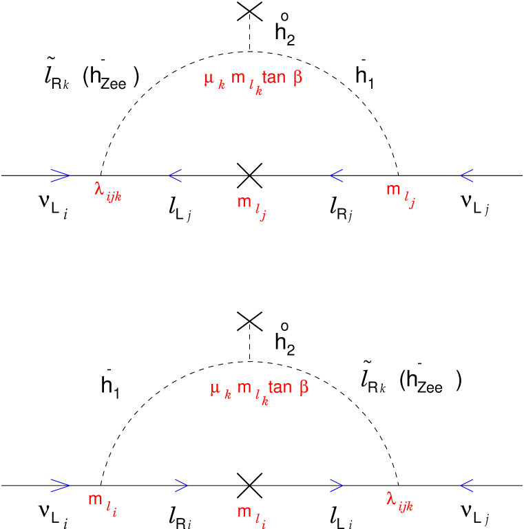
FIG. 1.: The two Feynman diagrams for the Zee mechanism in the $R$-parity violating SUSY framework. The original charged singlet boson $h_{\rm Zee}^{\mbox{-}}$ of the Zee model is shown in parentheses.

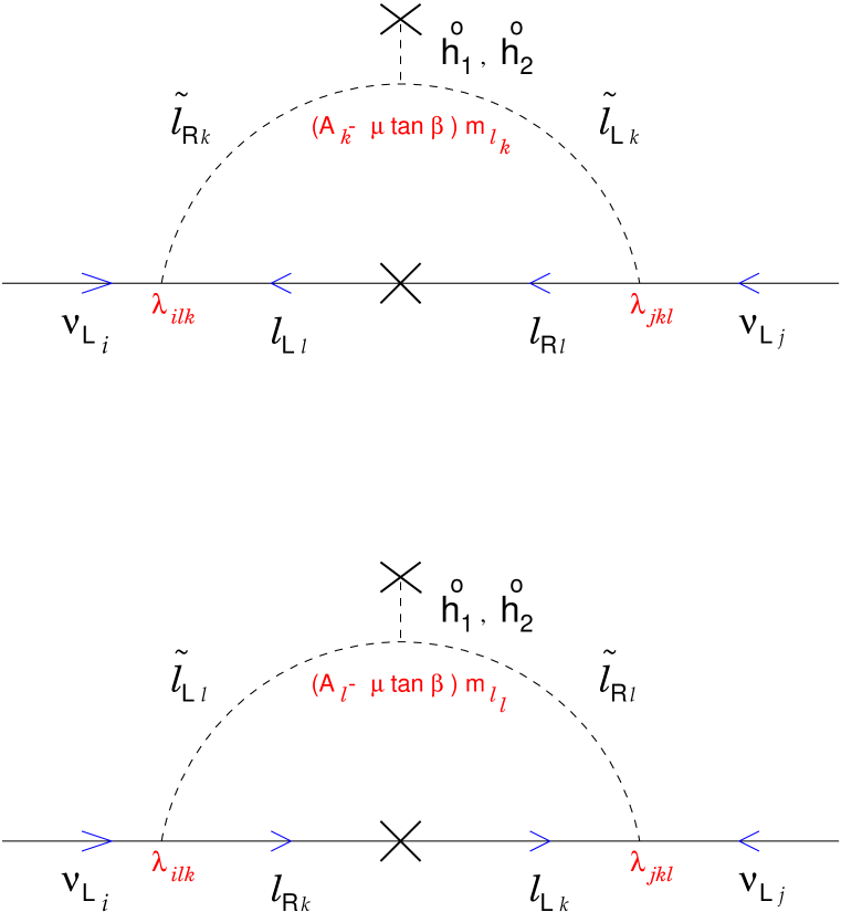
FIG. 2.: The one-loop diagrams for neutrino mass generated by the usual term $m_{\scriptscriptstyle\ell}\;(A^{\!\scriptscriptstyle E}-\mu\tan\beta)$ in $LR$ slepton mixing.

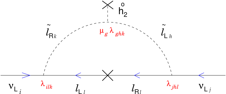
FIG. 3.: The one-loop diagram for neutrino mass generated by the term $\langle h_{\scriptscriptstyle 2}^{0}\rangle\,\mu_{g}\lambda_{ghk}\,\tilde{\ell}_{\scriptscriptstyle L_{h}}\tilde{\ell}^{*}_{\scriptscriptstyle R_{k}}$ in the $LR$ slepton mixing.

REFERENCES

• [1] Y. Fukuda et al. (Super-K Coll.), Phys. Rev. Lett. 81, 1562 (1998); Phys. Lett. B467, 185 (1999); Invited talk by Y. Totsuka (Super-K Coll.) at the XVth Particles and Nuclei International Conference, PANIC99, Uppsala, June 1999.
• [2] V. Barger, S. Pakvasa, T.J. Weiler, and K. Whisnant, Phys. Rev. D58, 093016 (1998); J.N. Bahcall, P.I. Krastev, and A. Yu. Smirnov, Phys. Rev. D58 096016 (1998); M.C. Gonzalez-Garcia, P.C. de Holanda, C. PeΓ±a-Garay, and J.W.F. Valle, FTUV/99-41, hep-ph/9906469.
• [3] LSND Collaboration, Phys. Rev. Lett. 75, 2650 (1995); ibid. 77, 3082 (1996); Phys. Rev. C58, 2489 (1998).
• [4] A. Zee, Phys. Lett. 93B, 389 (1980).
• [5] P. Frampton and S. Glashow, Phys. Lett. B461,95 (1999).
• [6] C. Jarlskog, M. Matsuda, S. Skadhauge, and M. Tanimoto, Phys. Lett. B449, 240 (1999).
• [7] N. Haba, M. Matsuda, and M. Tanimoto, hep-ph/9911511.
• [8] Y. Grossman and H. Haber, hep-ph/9906310.
• [9] For recent examples emphasizing on fitting neutrino oscillation data, see E. Chun, S. Kang, C. Kim, and U. Lee, Nucl. Phys. B544, 89 (1999); A. Abada and M. Losada, hep-ph/9908352; J. Romao, M. Diaz, M. Hirsch, W. Porod, and J. Valle, hep-ph/9907499; and Ref[11]. References to earlier works on neutrino mass from $R$-parity violation can also be found in the references listed in these papers.
• [10] M. Bisset, O. Kong, C. Macesanu, and L. Orr, Phys. Lett. B430, 274 (1998); hep-ph/9811498.
• [11] O. Kong, Mod. Phys. Lett. A14, 903 (1999).
• [12] S.T. Petcov, Phys. Lett. 115B, 401 (1982); M. Fukugita and T. Yanagida, Phys. Rev. Lett. 58, 1807 (1987); A. Yu. Smirnov and M. Tanimoto, Phys. Rev. D55, 1665 (1997); G.C. McLaughlin and J.N. Ng, TRI-PP-99-03, hep-ph/9903509.
• [13] Note that a major source of constraint from $\mu\to e\gamma$ in the general Zee model scenario is absent here as we have $f_{\scriptscriptstyle 23}=0$.
Refer to caption