Quark-binding effects in inclusive decays of heavy mesons

Abstract

We present a new approach to the analysis of quark-binding effects in inclusive decays of heavy mesons within the relativistic dispersion quark model. Various differential distributions, such as electron energy spectrum, $q^{2}$- and $M_{X}$-distributions, are calculated in terms of the $B$ meson soft wave function which also determines long-distance effects in exclusive transition form factors. Using the quark-model parameters and the $B$ meson wave function previously determined from the description of the exclusive $b\to u$ transitions within the same dispersion approach, we provide numerical results on various distributions in the inclusive $B\to X_{c}\ell\bar{\nu}_{\ell}$ decays.

I Introduction

Inclusive decays provide a promising possibility to determine the CKM matrix elements describing the mixing of $b$ quark, since a rigorous theoretical treatment of these decays, including nonperturbative effects, is possible. A consideration based on the Operator Product Expansion (OPE) and the Heavy Quark (HQ) expansion [1] allows one to connect the rate of the inclusive $B$ meson decay with the rate of the $b$ quark decay. An important consequence of the analysis based on the OPE is the appearance of the HQ binding effects in the integrated rates, both total and semileptonic (SL), of heavy meson decays only in the second order of the HQ expansion [2]. These second order corrections are expressed in terms of the two hadronic parameters, $\lambda_{1}$ and $\lambda_{2}$. The latter are the mesonic matrix elements of the operators of dimension 5 which appear in the OPE of the product of the two weak currents. The differential distributions can be calculated as expansions in inverse powers of HQ mass $m_{Q}$ [2, 3, 4].

Whereas presumably providing quite reliable results for the integrated SL decay rate, the OPE method encounters difficulties in calculating various differential distributions. For instance, before comparing the OPE-based results for the differential distributions with the true distributions a proper smearing over duality interval is necessary.

There are several reasons which yield complications in the calculation of some differential distributions, arising mostly in the resonance region near zero recoil, namely:

1. the duality-violating $1/m_{Q}$ effects (i.e. the difference between the true distributions and the smeared OPE results) in the differential distributions near zero recoil which originate from the delay in opening different hadronic channels, as noticed in [5]. Although these effects are cancelled in the integrated SL rate, they can considerably influence the kinematical distributions near the zero recoil point;

2. the convergence of the OPE series for the differential distributions persists only in the region where the quark produced in the SL decay is sufficiently fast. This means that the OPE cannot directly predict distributions in some kinematical regions, such as:

• the photon energy spectrum $d\Gamma/dE_{\gamma}$ in the radiative $B\to X_{s}\gamma$: the window in the photon energy between $m_{Q}/2$ and $M_{Q}/2$ turns out to be completely inaccessible within the OPE formalism [4];

• the lepton energy spectrum $d\Gamma/dE_{\ell}$ at large values of $E_{\ell}$ in semileptonic or rare leptonic decays;

• the lepton $q^{2}$-distributions in SL $B\to X_{c}~{}(X_{u})$ and rare $B\to X_{s}$ decays at large $q^{2}$ near zero recoil; in this region one encounters both the quark-binding and duality-violating effects.

Problems related to the quark-binding effects can be solved in principle by performing proper resummation of the nonperturbative corrections which in practice however leads to the appearance of a priori unknown distribution functions [6, 7].

The inclusion of the quark-binding effects in heavy meson decays was first done in [8], where an unknown distribution function of a heavy quark inside the heavy meson was introduced. Evidently, this distribution function is connected with the wave function of the heavy meson which also determines the exclusive transition form factors. To put this connection on a more solid basis, it is reasonable to consider the inclusive and exclusive processes within the same approach.

We argue in this paper that the constituent quark model (QM) can be used an efficient tool for calculating differential distributions in inclusive decays of heavy mesons, covering also kinematical regions where OPE cannot provide a rigorous treatment. Namely, the constituent quark model allows one to take into account quark-binding effects in inclusive heavy meson decays in terms of the meson soft wave function. The latter describes the heavy meson properties both in exclusive and inclusive processes and thus allows one to consider on the same ground long-distance effects in various kinds of hadronic processes.

Quark-model calculations of inclusive distributions are essentially based on the evaluation of the box diagram (see Fig. 1a later on) by introducing the heavy meson wave function in one way or another. To illustrate the basic features of such an approach as well as its advantages and limitations it suffices to consider the case of a nonrelativistic (NR) potential model with scalar currents. Inclusion of relativistic effects can be then performed.

Let us consider a weak transition induced by the scalar current $J=\bar{c}b$, where both $b$ and $c$ are heavy. To make the nonrelativistic treatment consistent we assume that

$$m_{b},m_{c}\gg\delta m\equiv m_{b}-m_{c}\gg\Lambda,$$ (1)

where $\Lambda$ is the typical scale of the quark binding effects in the heavy meson. In the NR theory the general expression for the hadronic tensor

$$W(q_{0},\vec{q}) = \frac{1}{\pi}{\rm Im}\int<B|T(J(x)J^{+}(0))|B>e^{-iqx}dx$$ (2)

is reduced to the form

$$W(q_{0},\vec{q})=\frac{1}{\pi}{\rm Im}<B|G_{c\bar{d}}(M_{B}-q^{0}-i0,\vec{q})|B>.$$ (3)

Here $G_{c\bar{d}}(E,\vec{q})=(\hat{H}_{c\bar{d}}(\vec{q})-E)^{-1}$ is the full Green function corresponding to the the full Hamiltonian operator of the $c\bar{d}$ system with the total momentum $\vec{q}$

$$\hat{H}_{c\bar{d}}(\vec{q})=m_{c}+m_{d}+\frac{(\hat{\vec{k}}+\vec{q})^{2}}{2m_{c}}+\frac{\hat{\vec{k}^{2}}}{2m_{d}}+V_{c\bar{d}}(\hat{r}).$$ (4)

Thus, the hadronic tensor is the average of the full $c\bar{d}$ Green function over the ground state of the full $b\bar{d}$ Hamiltonian

$$\hat{H}_{b\bar{d}}|B>=M_{B}|B>=(m_{b}+m_{d}+\epsilon_{B})|B>.$$ (5)

In the rest frame of the $B$-meson one has

$$\hat{H}_{b\bar{d}}=m_{b}+m_{d}+\frac{\hat{\vec{k}^{2}}}{2m_{b}}+\frac{\hat{\vec{k}^{2}}}{2m_{d}}+V_{b\bar{d}}(\hat{r})\equiv m_{b}+m_{d}+\hat{h}_{b\bar{d}}$$ (6)

The following relation provides a basis for performing the OPE in the NR potential model [9]

$$\hat{H}_{c\bar{d}}-(M_{B}-q^{0})=-(\delta m-\frac{\vec{q}^{2}}{2m_{c}}-q^{0})+\left[\hat{h}_{b\bar{d}}-\epsilon_{B}\right]+\frac{\hat{\vec{k}^{2}}+\hat{V}_{1}}{2}\left(\frac{1}{m_{c}}-\frac{1}{m_{b}}\right)-\frac{\hat{\vec{k}}\vec{q}}{m_{c}}+O\left(\frac{\gamma^{3}\delta m}{m_{c}^{3}}\right)$$ (7)

where $\gamma\sim\Lambda_{QCD}$ and we have assumed the following expansion of the potential

$$\hat{V}_{Q\bar{q}}=\hat{V}_{0}+\frac{\hat{V}_{1}}{2m_{Q}}+\frac{\hat{V}_{2}}{2m_{Q}^{2}}+...$$ (8)

Starting with (7) one constructs an OPE series using the amplitude of the free $b\to c$ quark transition as a zero-order approximation (hereafter referred to as the standard OPE). By virtue of the equations of motion, $\left(\hat{h}_{b\bar{d}}-\epsilon_{B}\right)|B>=0$ one observes the absence of $1/m_{Q}$ corrections to the leading order (LO) $b\to c$ amplitude, so that the corrections emerge only at the $1/m_{Q}^{2}$ order. Being completely reliable for the calculation of the integrated decay rate, this choice of the zero-order approximation turns out to be inconvenient however for calculating differential distributions. In particular, the distribution in the invariant mass of the produced hadronic system, $M_{X}$, becomes very singular and is represented via $\delta(M_{X}-m_{c})$ and its derivatives, such that the $1/m_{Q}$ corrections are even more singular than the LO result. This is the price one pays for the choice of the zero-order term.

It is clear that the free-quark transition amplitude is not the unique choice of the zero-order approximation, at least in quantum mechanics. For instance, another structure of the expansion can be obtained if the free $c\bar{d}$ Green function is used as the zero-order approximation.

In the NR quantum mechanics the relation between the full and the free Green functions is well known and reads

$$G^{-1}(E)=H-E,\quad G^{-1}_{0}(E)=H_{0}-E,\quad G^{-1}(E)-G^{-1}_{0}(E)=V,$$ (9)

or, equivalently,

$$G(E)=G_{0}(E)-G_{0}(E)VG(E)=G_{0}(E)-G_{0}(E)VG_{0}(E)+G_{0}(E)VG_{0}(E)VG_{0}(E)+...$$ (10)

For the heavy quark decay, in most of the kinematical $q^{2}$-region except for a vicinity of the zero recoil point, the Green function $G_{0}$ behaves as $1/m_{Q}$, and, since the matrix elements of the operator $V$ remain finite as $m_{Q}\to\infty$, the series (10) is an expansion in powers of $1/m_{Q}$. Notice that in the NR potential model the expansion (10) is fully equivalent to the OPE series obtained from (7). Inserting the expansion (10) into the expression for the hadronic tensor $W$ given by eq. (3), we come to the series shown in Fig 1.

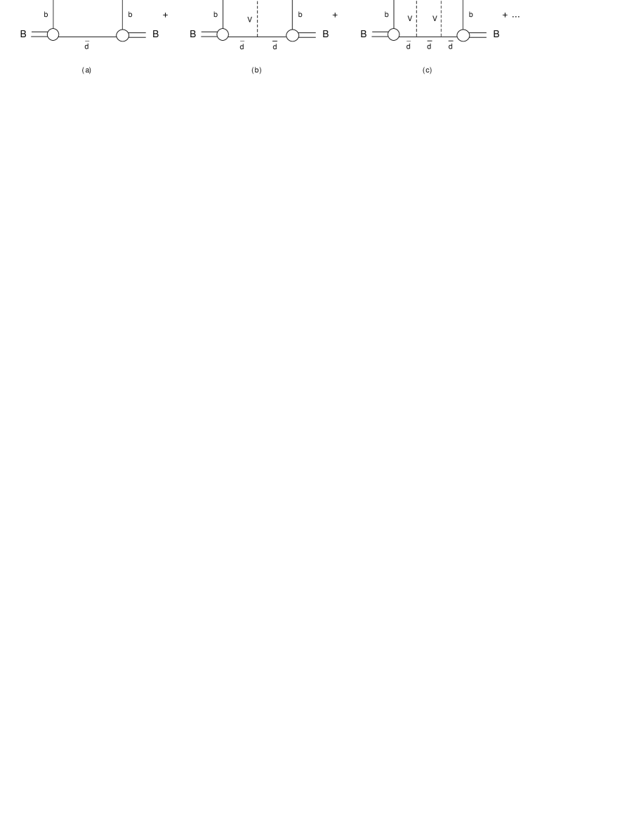
FIG. 1.: Expansion of the hadronic tensor in the quark model: (a) - the box diagram which provides the LO free-quark contribution, (b,c) - diagrams contributing in subleading $1/m_{Q}$ orders and containing the final state interaction $V\equiv V_{c\bar{d}}$. The short-dashed lines represent W bosons.

The LO term is the box diagram of Fig. 1a with the free $c$ and $\bar{d}$ quarks in the intermediate state. The corresponding analytical expression reads

$$W^{QM}=\frac{1}{\pi}{\rm Im}<B|G^{0}_{c\bar{d}}(M_{B}-q^{0},\vec{q})|B>.$$ (11)

This is the quantity usually taken into account in QM calculations. It is easy to see, that the SL decay rate calculation based on the box diagram of Fig. 1 only, reproduces the free quark SL decay rate in the HQ limit, but should contain also $1/m_{Q}$ corrections (see also the general structure of the QM results of Ref. [10]). Namely, the next-to-leading order (NLO) term in the expansion (10) is the diagram with a single insertion of the potential between the free $c$ and $\bar{d}$ quarks (the diagram of Fig. 1b). It has the order $1/m_{Q}$ and precisely cancels the $1/m_{Q}$ contribution of the QM box diagram, yielding in this way the absence of the $1/m_{Q}$ correction in the difference between the decay rates of bound and free heavy quarks.

Thus, the QM box-diagram calculation is just the first–order term in an alternative expansion of the full Green function: unlike the standard OPE series which starts from a single $c$-quark in the intermediate state, the QM starts from the free $c\bar{d}$ pair which is the eigenstate of the Hamiltonian

$$H^{0}_{c\bar{d}}(\vec{q})=m_{c}+m_{d}+\frac{(\vec{k}+\vec{q})^{2}}{2m_{c}}+\frac{\vec{k}^{2}}{2m_{d}}.$$ (12)

Hereafter we refer to the expansion of the decay rate based on the expansion (10) of the Green function as the QM expansion.

Summing up, the quark model provides an alternative $1/m_{Q}$ expansion with the following properties:

• the box diagram of Fig. 1a provides the LO $1/m_{Q}$ term and reproduces the free-quark decay in the limit $m_{Q}\to\infty$. All other terms contribute only in subleading $1/m_{Q}$ orders;

• the differential distributions in any $1/m_{Q}$ order are convergent for almost all allowed $q^{2}$, except for the region close to zero recoil;

• before comparing the calculated differential distributions based on the expansion (10) with the true distributions in the resonance region a proper smearing over some duality interval is required;

• the $1/m_{Q}$ correction to the LO term is nonvanishing.

Clearly, the properties 1-3 are completely equivalent to the standard OPE, while the property 4 makes the QM expansion much less convenient than the standard OPE, at least for the calculation of the SL decay rate. However:

• the expansion (10) turns out to be more suitable for the calculation of the differential distributions, e.g. for the calculation of $d\Gamma/dM_{X}$: in this case the LO result (the box diagram of Fig. 1a) is well-defined in the whole kinematical region as well as the higher order corrections to it. Thus already the box diagram is appropriate for comparison with the experimental $d\Gamma/dM_{X}$ at all $M_{X}$ apart from the resonance region. Beyond the resonance region no additional smearing of the calculated $d\Gamma/dM_{X}$ is required.

In full QCD the situation is of course much more complicated and hadrons are coherent states of infinite number of quarks and gluons. Nevertheless, many applications of the constituent quark model have proved the treatment of mesons as bound states of two constituent quarks to provide a reasonable description of their properties. From this viewpoint the arguments given above remain valid. Namely, the box diagram represents the main contribution to the hadronic tensor which reproduces the free-quark decay in the infinite quark mass limit. However hadronic tensor calculated from the box diagram contains the $1/m_{Q}$ term compared with the free-quark decay tensor. This linear $1/m_{Q}$ term is known to be cancelled by the $1/m_{Q}$ order contributions of higher order diagram and to be absent in the full expression. In practice, however the $1/m_{Q}$ term of the box diagram is not so dangerous: namely, the hadronic tensor calculated from the box diagram, as well as all corrections given by the other graphs, are regular in the whole kinematical region. Thus the box diagram should provide a reasonable description already appropriate for comparison with experiment. Moreover, the box-diagram result can be further improved by effectively taking into account the higher order term which kills the $1/m_{Q}$ correction contained in the box diagram. We follow this strategy in our analysis and perform a relativistic treatment of quark-binding effects within a constituent quark picture.

Our consideration of the quark binding effects in inclusive SL decays is based on the relativistic dispersion formulation of the quark model previously developed for the description of meson transition form factors [11]. Within this approach, the inclusive decay rates as well as the exclusive hadron transition form factors are given by double spectral representations in terms of the soft meson wave functions. The double spectral densities of these spectral representations are obtained from the corresponding Feynman graphs. The subtraction terms in spectral representations for exclusive transition form factors are fixed by requiring the structure of the HQ expansion in the QM to match the structure of the HQ expansion in QCD. In this paper we proceed along the same lines in inclusive processes.

Our main results are the following:

• we construct the double spectral representation of the hadronic tensor within the constituent quark model starting with $q^{2}<0$. The hadronic tensor is represented in terms of the soft wave function of the $B$ meson and the double spectral density of the box diagram. The hadronic tensor at $q^{2}>0$ is obtained by the analytical continuation. Then the $1/m_{Q}$ expansion of the spectral representation of the decay rate is performed and the LO term is shown to reproduce the free quark decay rate. The subtraction is defined in such a way that the $1/m_{Q}$ correction to the SL decay rate is absent. This corresponds to effectively taking into account other terms beyond the box-diagram approximation which contribute in subleading $1/m_{Q}$ orders. Moreover an approximate account of the $1/m_{Q}^{2}$ effects of the whole series within the box-diagram expression is possible. This is done by introducing a phenomenological cut in the double spectral representation of the box-diagram which affects only the differential distributions at large $q^{2}$. This cut brings the size of the $1/m_{Q}^{2}$ corrections in the $\Gamma(B\to X_{c}\ell\bar{\nu}_{\ell})$ in full agreement with the OPE result and keeps the LO and $1/m_{Q}$ correction unchanged. The cut yields differential distributions which are finite also in the endpoint $q^{2}$-region where the HQ expansion series is not properly convergent;

• various differential distributions are calculated in terms of the $B$-meson soft wave function. These distributions are regular in the whole kinematically accessible region and, apart from the resonance region (where the exact distributions are dominated by single resonances and a proper smearing over the duality intervals is necessary), can be directly compared with the observable values. The main effect of quark-binding upon these distributions is determined unambiguously through the soft wave function, while the $1/m_{Q}^{2}$ corrections depend on the particular details of an approximate account of the higher-order terms in the series (10). However, in practice these details are not essential due to the following two reasons: first they are numerically small, and second, the size of the $1/m_{Q}^{2}$ corrections in the integrated SL rate is close to the OPE result. So we expect that the size of the $1/m_{Q}^{2}$ corrections is reasonably reproduced also in other quantities;

• we perform numerical estimates of various differential distributions in inclusive decays in terms of the $B$-meson wave function known from the description of the exclusive processes [12, 13].

The paper is organized as follows: in the next section we present necessary formulas for the free-quark decay and also the OPE prediction for the total integrated rate up to $1/m_{Q}^{2}$ corrections. In Section 3 we construct the dispersion representation for the box diagram at $q^{2}<0$ and discuss its analytical continuation to $q^{2}>0$. Section 4 performs the $1/m_{Q}$ expansion of the hadronic tensor in the quark model, and Section 5 presents numerical results for differential distributions. Finally, a brief summary is given in the Conclusion.

II Free quark decay and OPE

Let the effective Hamiltonian governing the quark transition $Q\to Q^{\prime}$ with the emission of the particle $\phi$ have the following structure

$$H_{eff}(x)=\bar{Q}^{\prime}(x)\hat{\Gamma}Q(x)\phi(x)$$ (13)

where $\hat{\Gamma}$ denotes a relevant combination of the Dirac matrices. Following notations of ref [11] for the exclusive form factors, we denote the parent heavy quark $Q$ also as $Q_{2}$ and the daughter quark $Q^{\prime}$ as $Q_{1}$.

A tree-level rate of the free-quark decay initiated by this effective Hamiltonian averaged over the polarizations of the initial quark $Q_{2}$ and summed over polarizations of the final quark $Q_{1}$ has the form

$${d\Gamma_{0}\over dq^{2}} = \frac{(2\pi)^{4}}{2m_{2}}\int|T_{0}|^{2}\frac{dk_{1}dk_{\phi}}{(2\pi)^{6}}\delta(k_{1}^{2}-m_{1}^{2})\delta(k_{\phi}^{2}-q^{2})\delta(k_{2}-k_{1}-k_{\phi})$$ (14)

$$= \frac{(2\pi)^{4}}{2m_{2}(2\pi)^{6}}\frac{\pi\lambda^{1/2}(m_{2}^{2},m_{1}^{2},q^{2})}{2m_{2}^{2}}|T_{0}|^{2},$$ (15)

where $q^{2}$ is the mass squared of the particle $\phi$ and

$$|T_{0}|^{2}=\frac{1}{2}\sum_{\sigma}\bar{u}_{\sigma}(k_{2})\hat{\Gamma}(m_{1}+\hat{k}_{1})\hat{\Gamma}u_{\sigma}(k_{2})=\frac{1}{2}{\rm Sp}\left((m_{2}+\hat{k}_{2})\hat{\Gamma}(m_{1}+\hat{k}_{1})\hat{\Gamma}\right).$$ (16)

Hereafter we use the notation $\lambda(x,y,z)\equiv(x+y-z)^{2}-4xy$.

These formulas can be readily applied to the particular cases of radiative and SL decays. In the latter case one needs to multiply $d\Gamma_{0}/dq^{2}$ by the the leptonic tensor $L(q^{2})$ to obtain the full differential distribution $d\Gamma_{0}^{SL}/dq^{2}=d\Gamma_{0}/dq^{2}\cdot L(q^{2})$. Hereafter the inclusion of the leptonic tensor in the definition of $d\Gamma_{0}/dq^{2}$ is understood and we drop the superscript SL.

In the case of the SL $b\to c\ell\bar{\nu}_{\ell}$ transition the free-quark differential decay rate reads explicitly as (cf., e.g., [2, 3])

$${d\Gamma_{0}\over dq^{2}}={G_{F}^{2}|V_{bc}|^{2}\over 96\pi^{3}}\frac{1}{m_{b}^{3}}\lambda^{1/2}(m_{b}^{2},m_{c}^{2},q^{2})C(m_{b}^{2},m_{c}^{2},q^{2}),$$ (17)

where $G_{F}$ is the universal Fermi constant, $V_{bc}$ is the CKM matrix element, and

$$C(m_{b}^{2},m_{c}^{2},q^{2})=(m_{b}^{2}-m_{c}^{2})^{2}+q^{2}(m_{b}^{2}+m_{c}^{2})-2q^{4}.$$ (18)

The integrated SL rate is then given by

$$\Gamma_{0}=\int_{0}^{(m_{b}-m_{c})^{2}}dq^{2}{d\Gamma_{0}\over dq^{2}}={G_{F}^{2}|V_{bc}|^{2}\over 192\pi^{3}}\cdot m_{b}^{5}\cdot I_{0}(r)$$ (19)

with $I_{0}(r)=1-8r+8r^{3}-r^{4}-12r^{2}{\rm ln}(r)$, $r\equiv(m_{c}/m_{b})^{2}$.

The OPE predicts that in the decay of the heavy meson, the $1/m_{b}$ corrections to the free quark rate (19) are absent, and up to $1/m_{b}^{2}$ terms the integrated SL rate is given by (cf., e.g., [2, 3])

$$\Gamma=\Gamma_{0}\cdot\left[1+{\lambda_{1}+3\lambda_{2}\over 2m_{b}^{2}}-6{\lambda_{2}\over m_{b}^{2}}{(1-r)^{4}\over I_{0}(r)}\right].$$ (20)

Here $\lambda_{1}$ and $\lambda_{2}$ are the hadronic matrix elements of the operators of dimension 5 appearing in the OPE of the product of the two weak currents. The value $\lambda_{2}=0.12~{}GeV^{2}$ is well known from the $B-B^{*}$ mass splitting, whereas the knowledge of $\lambda_{1}$ is loose and present estimates range from $-0.6~{}GeV^{2}$ to $0$. Note that in the NR quark potential model one has $\lambda_{1}=-<\vec{k}^{2}>$, where $\vec{k}$ is the relative momentum of the constituent $Q\bar{q}$ pair (cf, e.g., [14]). Typically, the NR quark model estimates of $\lambda_{1}$ range from $-0.6$ to $-0.4~{}GeV^{2}$.

III Inclusive meson decay in the quark model

We now proceed to the calculation of the inclusive rate for the decay of a pseudoscalar meson with mass $M_{1}$ containing a heavy quark $Q_{2}$, which we will refer to as $P_{Q_{2}}$, induced by the quark transition (13).

We start with the box diagram of Fig. 1a. Our notations shown in Fig 2 follow those of ref [11] where transition form factors within the similar dispersion approach have been considered.

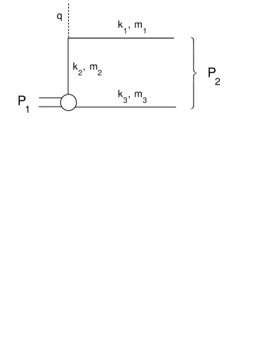
FIG. 2.: Momentum notations in the box diagram.

The decay rate corresponding to this diagram can be written in the form

$${d\Gamma(P_{Q_{2}}\to X_{Q_{1}}\phi)\over dq^{2}}=\frac{(2\pi)^{4}}{2M_{1}}\int\frac{dk_{1}dk_{3}dk_{\phi}}{(2\pi)^{9}}|T|^{2}\delta(k_{1}^{2}-m_{1}^{2})\delta(k_{3}^{2}-m_{3}^{2})\delta(k_{\phi}^{2}-q^{2})\delta(p_{1}-k_{2}-k_{3}-k_{\phi}),$$ (21)

where $T$ is the amplitude of the meson decay $P_{Q_{2}}\to Q_{1}\bar{q}_{3}\phi$.

In the dispersion approach the decay rate can be written in the form of the following spectral representation:

$${d\Gamma(P_{Q_{2}}\to X_{Q_{1}}\phi)\over dq^{2}}=\frac{(2\pi)^{4}}{2M_{1}}\int\frac{ds_{1}\;ds_{2}}{(s_{1}-M_{1}^{2})^{2}}\frac{\pi\lambda^{1/2}(s_{1},s_{2},q^{2})}{2s_{1}}\tilde{A}(s_{1},s_{2},q^{2})$$ (22)

where the spectral density $\tilde{A}(s_{1},s_{2},q^{2})$ is connected with the double discontinuity of the box diagram shown in Fig. 1.

The amplitude $A$ of Fig. 1a depends on six Lorentz scalar variables $p_{1}^{2},p^{\prime 2}_{1},p^{2}_{2},q^{2},q^{\prime 2},\kappa^{2}$, where the momenta satisfy the following relations $p_{1}-p^{\prime}_{1}=q-q^{\prime}=\kappa$, and $p_{1}-q=p^{\prime}_{1}-q^{\prime}=p_{2}$. The amplitude can be written as double spectral representation in $p_{1}^{2}$ and $p^{\prime 2}_{1}$

$$A(p_{1}^{2},p^{\prime 2}_{1},p^{2}_{2},q^{2},q^{\prime 2},\kappa^{2})=\int\frac{ds_{1}}{s_{1}-p_{1}^{2}}\frac{ds^{\prime}_{1}}{s^{\prime}_{1}-p^{\prime 2}_{1}}\tilde{A}(s_{1},s^{\prime}_{1},p^{2}_{2},q^{2},q^{\prime 2},\kappa^{2}).$$ (23)

In this equation $\tilde{A}$ is the full spectral density of the amplitude and includes properly defined subtraction terms. The spectral density $\tilde{A}$ is calculated from the double discontinuity $\tilde{A}_{D}$,

$$\tilde{A}_{D}=\frac{1}{(2\pi i)^{2}}{\rm disc}_{s_{1}}{\rm disc}_{s^{\prime}_{1}}A(s_{1},s^{\prime}_{1},p^{2}_{2},q^{2},q^{\prime 2},\kappa^{2}),$$ (24)

through a relevant subtraction procedure.

A The spacelike region

The double discontinuity $\tilde{A}_{D}$ of the box diagram of Fig. 1a can be calculated at $q^{2}\leq 0$ and $q^{\prime 2}\leq 0$ by placing all intermediate quarks on their mass shells but keeping the initial and final mesons virtual and having the masses squared $s_{1}$ and $s_{1}^{\prime}$, respectively. To obtain the corresponding expression at positive values of $q^{2}=q^{\prime 2}$ which is necessary e.g. for SL decays, we shall perform the analytical continuation in $q^{2}$. At $q^{2},~{}q^{\prime 2}\leq 0$ the procedure explained in detail in [11] yields the expression

$$\tilde{A}_{D}(s_{1},s^{\prime}_{1},s_{2},q^{2},q^{\prime 2},\kappa^{2}) = \frac{1}{(2\pi)^{9}}\int dk_{1}dk_{2}dk^{\prime}_{2}dk_{3}\delta(k_{1}^{2}-m_{1}^{2})\delta(k_{2}^{2}-m_{2}^{2})\delta(k^{\prime 2}_{2}-m_{2}^{2})\delta(k_{3}^{2}-m_{3}^{2})$$ (27)

$$\times\delta(\tilde{p}_{1}-k_{2}-k_{3})\delta(\tilde{p}^{\prime}_{1}-k^{\prime}_{2}-k_{3})\delta(\tilde{p}_{2}-k_{1}-k_{3})$$

$$\times(-1){\rm Sp}\left(i\gamma_{5}\,G(s_{1})\,(m_{3}-\hat{k}_{3})i\gamma_{5}\,G(s^{\prime}_{1})\,(m_{2}+\hat{k}_{2})\hat{\Gamma}(m_{1}+\hat{k}_{1})\hat{\Gamma}(m_{2}+\hat{k}_{2})\right),$$

where the momenta satisfy the following relations $\tilde{p}^{\prime}_{1}=\tilde{p}_{1}+\kappa$, $\tilde{q}^{\prime}=\tilde{q}+\kappa$, $\tilde{p}_{2}=\tilde{p}_{1}-\tilde{q}$, $\tilde{p}_{1}^{2}=s_{1}$, $\tilde{p}^{\prime 2}_{1}=s^{\prime}_{1}$, $\tilde{q}^{2}=q^{2}$, $\tilde{q}^{\prime 2}=q^{\prime 2}$, $\tilde{p}^{2}_{2}=s_{2}$. Notice that the quark structure of the (virtual) pseudoscalar meson transition into two real quarks is described by the vertex $G(s_{1})\bar{Q}_{2}(k_{2})i\gamma_{5}q_{3}(k_{3})\delta(\tilde{p}_{1}-k_{2}-k_{3})$, where $\tilde{p}_{1}^{2}=s_{1},k_{2}^{2}=m_{2}^{2},k_{3}^{2}=m_{3}^{2}$.

The spectral density $\tilde{A}(s_{1},s_{2},q^{2})$ in (22) is connected with the forward double spectral density of the box diagram $\tilde{A}(s_{1},s_{1}^{\prime},s_{2},q^{2},q^{\prime 2},\kappa^{2})$ as follows

$$\lim_{\kappa^{2}\to 0}\;\tilde{A}(s_{1},s_{1}^{\prime},s_{2},q^{2},q^{2},\kappa^{2})=\delta(s_{1}-s_{1}^{\prime})\tilde{A}(s_{1},s_{2},q^{2}).$$ (28)

The form of the subtraction procedure in the spectral representation (23) cannot be determined within the dispersion approach and should be fixed from some other arguments. We can determine the subtraction term by requiring the absence of the $1/m_{Q}$ corrections in the ratio of the bound and free quark decay rates. As we have discussed, this corresponds to taking into account the $1/m_{Q}$ terms of other diagrams which are known to cancel the $1/m_{Q}$ term in the bix diagram. Our subtraction prescription explicitly reads

$$\tilde{A}(s_{1},s_{2},q^{2})=\frac{M_{1}}{\sqrt{s_{1}}}\tilde{A}_{D}(s_{1},s_{2},q^{2})$$ (29)

where $\tilde{A}_{D}$ is connected with the double discontinuity of the forward amplitude

$$\lim_{\kappa^{2}\to 0}\;\tilde{A}_{D}(s_{1},s_{1}^{\prime},s_{2},q^{2},q^{2},\kappa^{2})=\delta(s_{1}-s_{1}^{\prime})\tilde{A}_{D}(s_{1},s_{2},q^{2}).$$ (30)

Explicit calculations give for $\tilde{A}_{D}$ the following expression

$$\bar{A}_{D}(s_{1},s_{2},q^{2})=\frac{\pi\theta(...)}{2\lambda^{1/2}(m_{1}^{2},m_{2}^{2},q^{2})}(-{\rm Sp}).$$ (31)

Notice that the argument of the $\theta$ function in eq (31) is just the same as for the spectral density of the triangle graph describing the form factor in the dispersion approach which can be read off from [11]. Since all quarks are on their mass shell, the trace can be rewritten in the following form

$$-{\rm Sp}=2|T_{0}|^{2}(s_{1}-(m_{2}-m_{3})^{2}),$$ (32)

where $|T_{0}|^{2}$ is just the square of the free-quark amplitude of eq (16). Finally, isolating the free-quark decay amplitude and solving the kinematical $\theta$ function we come to the following dispersion representation for the differential inclusive decay rate at $q^{2}\leq 0$

$${d\Gamma\over dq^{2}}=K_{0}(q^{2})\int ds_{1}\frac{G^{2}(s_{1})}{(s_{1}-M_{1}^{2})^{2}}\frac{s_{1}-(m_{2}-m_{3})^{2}}{8\pi^{2}s_{1}}\frac{m_{2}}{\sqrt{s_{1}}}\frac{m_{2}^{2}}{\lambda^{1/2}(m_{1}^{2},m_{2}^{2},q^{2})}\int_{s_{2}^{-}(s_{1},q^{2})}^{s_{2}^{+}(s_{1},q^{2})}ds_{2}\lambda^{1/2}(s_{1},s_{2},q^{2}),$$ (33)

where

$$K_{0}(q^{2})\equiv\frac{1}{\lambda^{1/2}(m_{2}^{2},m_{1}^{2},q^{2})}\frac{d\Gamma_{0}}{dq^{2}}=\frac{G_{F}^{2}|V_{21}|^{2}}{96\pi^{3}}\frac{C(m_{2}^{2},m_{1}^{2},q^{2})}{m_{2}^{3}}.$$ (34)

The limits $s_{2}^{\pm}$ are obtained by setting $\eta=\pm 1$ in the equation

$$s_{2}(s_{1},q^{2}) = (m_{1}+m_{3})^{2}+\frac{m_{1}}{m_{2}}\left(s_{1}-(m_{2}+m_{3})^{2}\right)+\frac{m_{1}}{m_{2}}(\omega-1)(s_{1}-m_{2}^{2}-m_{3}^{2})$$ (35)

$$+ \eta\frac{m_{1}}{m_{2}}\lambda^{1/2}(s_{1},m_{2}^{2},m_{3}^{2})\sqrt{\omega^{2}-1},$$ (36)

where the quark recoil $\omega$ is defined as follows

$$q^{2}=(m_{2}-m_{1})^{2}-2m_{1}m_{2}(\omega-1).$$ (37)

Note that in eq (33) the free-quark differential rate $d\Gamma_{0}/dq^{2}$ factorizes out, so that the differential rate for a bound quark is a product of the free-quark differential rate and a bound state factor, as already noted in [10]. Hereafter we use the notation $\varphi(s)=G(s)/(s-M_{1}^{2})$. The normalization condition of the soft wave function $\varphi(s)$ obtained from the elastic vector form factor of the heavy meson at $q^{2}=0$ reads [11]

$$\int ds_{1}\varphi^{2}(s_{1})\left[s_{1}-(m_{2}-m_{3})^{2}\right]\frac{\lambda^{1/2}(s_{1},m^{2}_{2},m_{3}^{2})}{8\pi^{2}s_{1}}=1.$$ (38)

It is convenient to rearrange eq (33) by isolating under the integral the structure similar to the structure of the normalization condition (38)

$${d\Gamma\over dq^{2}} = K_{0}(q^{2})\int ds_{1}\varphi^{2}(s_{1})\left[s_{1}-(m_{2}-m_{3})^{2}\right]\frac{\lambda^{1/2}(s_{1},m^{2}_{2},m_{3}^{2})}{8\pi^{2}s_{1}}\rho(s_{1},q^{2}),$$ (39)

$$\rho(s_{1},q^{2}) = \frac{m_{2}}{\sqrt{s_{1}}}\frac{m_{2}^{2}}{\lambda^{1/2}(s_{1},m^{2}_{2},m_{3}^{2})\lambda^{1/2}(m^{2}_{2},m_{1}^{2},q^{2})}\int_{s_{2}^{-}}^{s_{2}^{+}}ds_{2}\lambda^{1/2}(s_{1},s_{2},q^{2}).$$ (40)

As we shall see later, $\rho(s_{1},q^{2})\sim\lambda^{1/2}(m^{2}_{2},m_{1}^{2},q^{2})$ in the HQ limit, so that thanks to the normalization (38) of the soft wave function one gets $d\Gamma/dq^{2}\to d\Gamma_{0}/dq^{2}$ as $m_{Q}\to\infty$.

B The timelike region and the anomalous contribution

To obtain the spectral representation at $q^{2}>0$ we perform the analytical continuation in $q^{2}$. This procedure is done along the same lines as in the case of the transition form factor which has been discussed in detail in [11]. As a result of this procedure in addition to the normal part which is just the expression (39) taken at $q^{2}>0$, an anomalous part emerges due to the non-Landau type singularities of the Feynman graph. Thus, in the region $q^{2}\leq(m_{2}-m_{1})^{2}$ the representation for $\rho(s_{1},q^{2})$ takes the form

$$\rho(s_{1},q^{2}) = \frac{m_{2}}{\sqrt{s_{1}}}\frac{m_{2}^{2}}{\lambda^{1/2}(s_{1},m^{2}_{2},m_{3}^{2})\lambda^{1/2}(m^{2}_{2},m_{1}^{2},q^{2})}$$ (42)

$$\times\left[{\int_{s_{2}^{-}(s_{1},q^{2})}^{s_{2}^{+}(s_{1},q^{2})}ds_{2}\lambda^{1/2}(s_{1},s_{2},q^{2})+2\theta(q^{2})\theta(s_{1}>s_{1}^{0})\int_{s_{2}^{+}(s_{1},q^{2})}^{s_{2}^{L}(s_{1},q^{2})}ds_{2}\lambda^{1/2}(s_{1},s_{2},q^{2})}\right],$$

where

$$s_{2}^{L}(s_{1},q^{2}) = (\sqrt{s_{1}}-\sqrt{q^{2}})^{2},$$ (43)

$$\sqrt{s_{1}^{0}(q^{2})} = \frac{q^{2}+m_{2}^{2}-m_{1}^{2}}{2\sqrt{q^{2}}}+\sqrt{\left({\frac{q^{2}+m_{2}^{2}-m_{1}^{2}}{2\sqrt{q^{2}}}}\right)^{2}+m_{3}^{2}-m_{2}^{2}}.$$ (44)

The $q^{2}$-behavior of the anomalous term is determined by the lower limit of the $s_{1}$ integration, $s^{0}_{1}(q^{2})$. Namely, its contribution to the SL rate reads

$$\frac{1}{\Gamma}\frac{d\Gamma^{anom}}{d\omega}\simeq\frac{\Lambda^{3}}{m_{Q}^{3}\sqrt{\omega-1}}R^{anom}(\omega),$$ (45)

where

$$R^{anom}(\omega)=\int\limits_{\frac{m_{Q}^{2}}{\Lambda^{2}}(\omega-1)}^{\infty}d\vec{k}^{2}\Psi^{2}_{B}(\vec{k}^{2}).$$ (46)

Here $|\vec{k}|=\lambda^{1/2}(s_{1},m_{2}^{2},m_{3}^{2})/2\sqrt{s_{1}}$ is the relative momentum of the quarks inside the $B$-meson, and the wave function $\Psi_{B}(\vec{k}^{2})$ can be expressed through $\varphi(s)$ [11]. In terms of $\Psi_{B}(\vec{k}^{2})$ the normalization condition (38) takes the form $\int\Psi_{B}^{2}(\vec{k}^{2})d\vec{k}^{2}=1$ such that $R^{anom}(1)=1$. Since the soft wave function is steeply falling beyond the confinement region where $\vec{k}^{2}\mathrel{\hbox to0.0pt{\lower 4.0pt\hbox{\hskip 1.0pt$\sim$}\hss}\raise 1.0pt\hbox{$<$}}\Lambda^{2}$, the anomalous contribution becomes inessential already at $\omega-1\simeq\Lambda/m_{b}$. Only in the endpoint region $\omega-1\mathrel{\hbox to0.0pt{\lower 4.0pt\hbox{\hskip 1.0pt$\sim$}\hss}\raise 1.0pt\hbox{$<$}}\frac{\Lambda^{2}}{m_{Q}^{2}}$ the anomalous contribution to the differential distribution becomes strong and diverges like $\frac{1}{\Gamma}\frac{d\Gamma^{anom}}{d\omega}\simeq\frac{\Lambda^{3}}{m_{Q}^{3}}\frac{1}{\sqrt{\omega-1}}$.

The contribution of the anomalous term to the integrated SL rate is $\Gamma^{anom}/\Gamma\simeq\Lambda^{2}/m_{Q}^{2}$ and comes from the endpoint region, whereas the rest of the phase space $0<q^{2}\mathrel{\hbox to0.0pt{\lower 4.0pt\hbox{\hskip 1.0pt$\sim$}\hss}\raise 1.0pt\hbox{$<$}}\Lambda/m_{Q}$ provides only the relative $\Lambda^{3}/m_{Q}^{3}$ anomalous contribution to the SL decay rate.

Therefore, the anomalous contribution is negligible at all $\omega$ except for the endpoint region $\omega-1\mathrel{\hbox to0.0pt{\lower 4.0pt\hbox{\hskip 1.0pt$\sim$}\hss}\raise 1.0pt\hbox{$<$}}\frac{\Lambda^{2}}{m_{Q}^{2}}$, which is in fact a very narrow region near zero recoil. As we have discussed, the HQ expansion for the differential distributions is anyway ill-defined in this kinematical region. Contributions of the same order of magnitude come also from other terms in the expansion (10), and keeping this anomalous contribution is beyond the accuracy of our considerations. Thus we shall systematically omit the anomalous contribution in numerical calculations.

IV The heavy quark expansion of the inclusive decay rate in the quark model

In this section we perform the HQ expansion of the meson inclusive decay rate. We show that:

• in the LO the heavy meson inclusive decay rate is equal to the free quark decay rate;

• our subtraction prescription (29) leads to the differential distribution $d\Gamma/dq^{2}$ given by eq (39) which satisfies the relation $(d\Gamma(B\to X_{c}\ell\bar{\nu}_{\ell})/dq^{2})/(d\Gamma(b\to c\ell\bar{\nu}_{\ell})/dq^{2})=1+O(1/m_{Q}^{2})$ in most of the $q^{2}$ region except for a close vicinity of zero recoil point. This property guarantees the absence of the $1/m_{Q}$ in the ratio of the integrated rates, i.e. $\Gamma(B\to X_{c}\ell\bar{\nu}_{\ell})/\Gamma(b\to c\ell\bar{\nu}_{\ell})=1+O(1/m_{Q}^{2})$;

• the size of the $1/m_{Q}^{2}$ corrections can be tuned such that they become numerically close to the OPE prediction. This is done by introducing the cut in the spectral representation of the decay rate of the $B$ meson. This cut affects only the differential distribution $d\Gamma(B\to X_{c}\ell\bar{\nu}_{\ell})/dq^{2}$ at large $q^{2}$ near zero recoil, i.e. in the region $\omega\leq 1+O(1/m_{Q})$.

The most important feature of the whole approach is that already the zero order expression provides a realistic $M_{X}$-distribution. Modifications b) and c) while affecting the total rate and the $q^{2}$-distributions at large $q^{2}$, only moderately affect the $M_{X}$-distribution, so that the latter is mostly determined only by the soft $B$-meson wave function.

A Soft wave function and normalization condition

First, we need to specify the properties of the soft meson wave function. A basic property of the soft wave function $\varphi(s,m_{Q},m_{\bar{q}},\Lambda)$ is its strong peaking in terms of the relative quark momentum in the region of the order of $\Lambda\simeq\Lambda_{QCD}$.

For elaborating the $1/m_{Q}$ expansion, it is convenient to formulate such peaking in terms of the variable $z$ such that $s=(m_{Q}+m_{3}+z)^{2}$ (hereafter we denote the mass of the light spectator quark as $m_{3}$). In the heavy meson, the variable $z$ is related to the relative quark momentum as follows

$${\vec{k}}^{2}=z(z+2m_{3})+O(1/m_{Q}).$$ (47)

Hence, a localization of the soft wave function in terms of $z$ means that the wave function is nonzero as $z\leq\Lambda$. In the heavy meson case we imply that $m_{Q}\gg m_{3}\simeq z\simeq\Lambda$.

The normalization condition (38) is a consequence of the vector current conservation in the full theory and it provides an (infinite) chain of relations at different $1/m_{Q}$ orders. Namely, expanding the soft wave function in $1/m_{Q}$ as follows

$$\varphi(s,m_{Q},m_{3},\Lambda)=\frac{\pi}{\sqrt{m_{Q}}}\phi_{0}(z,m_{3},\Lambda)\left[{1+\frac{m_{3}}{4m_{Q}}\chi_{1}(z,m_{3},\Lambda)+O(1/m_{Q}^{2})}\right],$$ (48)

we come to the normalization condition in the form

$$\int dz\phi^{2}_{0}(z)\sqrt{z}(z+2m_{3})^{3/2}\left[1+\frac{m_{3}}{2m_{Q}}\chi_{1}(z)-\frac{m_{3}}{2m_{Q}}+\ldots\right]=1.$$ (49)

This exact relation is equivalent to an infinite chain of equations in different $1/m_{Q}$ orders. Lowest order relations take the form

$$\int dz\;\phi^{2}_{0}(z)\sqrt{z}(z+2m_{3})^{3/2}=1,$$ (50)

$$\int dz\;\phi^{2}_{0}(z)\sqrt{z}(z+2m_{3})^{3/2}\chi_{1}(z)=1,etc.$$ (51)

In particular, the Isgur-Wise function is given by the following expression through $\phi_{0}$

$$\xi(\omega)=\int dz_{1}\phi_{0}(z_{1})\sqrt{z_{1}(z_{1}+2m_{3})}\int\limits_{-1}^{1}\frac{d\eta}{2}\phi_{0}(z_{2})\left({m_{3}+\frac{2m_{3}+z_{1}+z_{2}}{1+\omega}}\right).$$ (52)

The expression for $z_{2}$ through $z_{1}$ and $\eta$ ($-1\leq\eta\leq 1$) is obtained by expanding (35) in $1/m_{Q}$

$$z_{2} = z_{1}+(z_{1}+m_{3})(\omega-1)+\eta\sqrt{z_{1}(z_{1}+2m_{3})}\sqrt{\omega^{2}-1}+O(1/m_{Q}),$$ (53)

and for the calculation of the IW function only the LO part of this relation should be used.

B The HQ expansion

First let us consider the HQ expansion of the unsubtracted quantity $\rho_{D}$. The normal part of $\rho_{D}(s_{1},q^{2})$ reads

$$\rho_{D}(s_{1},q^{2})=\frac{m_{2}}{M_{1}}\int_{-1}^{1}\frac{d\eta}{2}\lambda^{1/2}(s_{1},s_{2},q^{2}).$$ (54)

This representation is a convenient starting point for performing the HQ expansion. Notice that although the integration in $\eta$ can be easily performed, it is more convenient to work out the HQ expansion before the integration.

Assuming that $m_{2}$ is large and that the meson wave function is localized in the region $z_{1}\simeq\Lambda$ we obtain the following expression for $\lambda(s_{1},s_{2},q^{2})$ valid at all $q^{2}$

$$\lambda(s_{1},s_{2},q^{2}) \to m_{2}^{4}\left({1+\frac{z+m_{3}}{m_{2}}}\right)^{2}\left[{\lambda(1,\hat{q}^{2},\hat{r}^{2})+\frac{2\eta}{m_{2}}\chi(z)\sqrt{z(z+2m_{3})}(1+\hat{q}^{2}-\rho^{2})\lambda^{1/2}(1,\hat{q}^{2},\hat{r}^{2})}\right.$$ (56)

$$\left.{+\frac{z(z+2m_{3})}{m_{2}^{2}}(1+\hat{q}^{2}-\hat{r}^{2})^{2}+\frac{\eta^{2}}{m_{2}^{2}}z(z+2m_{3})\lambda(1,\hat{q}^{2},\hat{r}^{2})}\right]$$

where $\hat{q}^{2}=q^{2}/m_{b}^{2}$, $\hat{r}=m_{1}/m_{2}$ and $\chi(z)=1-(z+m_{3})/2m_{2}$. In the limit $m_{2}\to\infty$ we can expand the $\lambda(s_{1},s_{2},q^{2})$ in powers of $1/m_{2}$. Notice however that an actual expansion parameter is not $1/m_{2}$ but rather

$$\frac{\sqrt{z(z+2m_{3})}}{m_{2}\lambda^{1/2}(1,\hat{q}^{2},\hat{r}^{2})},$$ (57)

and the averaging over the $B$ meson state implies $\sqrt{z(z+2m_{3})}\simeq\Lambda$. Hence the region where the expansion is fastly converging is $m_{2}\lambda^{1/2}(1,\hat{q}^{2},\hat{r}^{2})\gg\Lambda$. This relation can be written as $|\vec{k}_{1}|=\lambda^{1/2}(m_{2}^{2},m_{1}^{2},q^{2})/2m_{2}\gg\Lambda$, which means that in the rest frame of the $b$ quark the daughter quark has a 3-momentum much bigger than $\Lambda$.

The final expression reads

$$\rho_{D}(s_{1},q^{2})\to\lambda^{1/2}(m_{1}^{2},m_{2}^{2},q^{2})\frac{m_{2}}{M_{1}}\left({1+\frac{z+m_{3}}{m_{2}}}\right)\left[{1+\frac{z(z+2m_{3})}{2m_{2}^{2}}\left({1+\frac{8\hat{q}^{2}}{3\lambda(1,\hat{q}^{2},\hat{r}^{2})}}\right)}\right].$$ (58)

The $1/m_{Q}$ term in the ratio of the bound to free quark distributions is generated by the $(m_{2}+z+m_{3})/M_{1}$ term in $\rho_{D}$.

As we have discussed this linear $1/m_{Q}$ term contained in the box diagram cancels against the $1/m_{Q}$ terms coming from other terms in the expansion (10). Thus the main contribution of these other terms in the series (10) can be taken into account by performing the subtraction in the spectral representation of the box diagram which kills the $1/m_{Q}$ term as follows:

$$\rho(s_{1},q^{2})=\frac{M_{1}}{\sqrt{s_{1}}}\rho_{D}(s_{1},q^{2}).$$ (59)

In the HQ limit $z(z+2m_{3})=\vec{k}^{2}$, so after performing the subtraction we come to the following relation

$$R(q^{2})\equiv\frac{d\Gamma(B\to X_{c}\ell\bar{\nu}_{\ell})/dq^{2}}{d\Gamma(b\to c\ell\bar{\nu}_{\ell})/dq^{2}}\to 1+\frac{<\vec{k}^{2}>}{2m_{2}^{2}}\left({1+\frac{8\hat{q}^{2}}{3\lambda(1,\hat{q}^{2},\hat{r}^{2})}}\right).$$ (60)

This expansion is valid in the region of $q^{2}$ such that $\lambda(1,\hat{q}^{2},\hat{r}^{2})=O(1)$, i.e. in most of the $q^{2}$ phase space except for the region near zero recoil where $\lambda(1,\hat{q}^{2},\hat{r}^{2})\simeq 0$.

The expression (60) has the following features:

• in the LO the ratio $R(q^{2})$ is equal to one and thus the decay rate of the free and the bound quark coincide in the HQ limit at all $q^{2}$. Moreover, the differential distribution also coincide within the $1/m_{Q}$ accuracy in most of the $q^{2}$ phase space, except for the region near zero recoil. This guarantees the absence of the $1/m_{Q}$ corrections in the ratio of the integrated rates as well. Thus, our description is in full agreement with the OPE results within the $1/m_{Q}$ order;

• since the box diagram represents only a part of the $1/m_{Q}^{2}$ corrections, we cannot expect the box diagram alone to reproduced correctly the $1/m_{Q}^{2}$ term in the ratio of the integrated rates $\Gamma/\Gamma_{0}$. In fact, the sign of the $1/m_{Q}^{2}$ correction in eq. (60) turns out to be opposite to the OPE result (cf., e.g., with the results of refs. [2, 3] at $q^{2}=0$). Moreover, the whole $1/m_{Q}^{2}$ effect in the box diagram is expressed only in terms of $<\vec{k}^{2}>$, whereas the $1/m_{Q}^{2}$ corrections of the whole series contains also $<\hat{V}_{1}>$ [14], where $\hat{V}_{1}$ is the $1/m_{Q}$ term appearing in the expansion (8) of the effective potential (e.g., the chromomagnetic operator in QCD).

We argue however that it is possible to further modify the spectral representation of the box diagram to bring the size of the $1/m_{Q}^{2}$ term developed by this modified representation in agreement with the OPE result. This procedure corresponds to phenomenologically taking into account the contribution of other $1/m_{Q}^{2}$ terms of the expansion (10).

Omitting the anomalous contribution as discussed previously, the differential decay rate reads

$$\frac{d\Gamma}{dq^{2}} = K_{0}(q^{2})\int_{(m_{1}+m_{3})^{2}}^{\infty}ds_{1}\varphi^{2}(s_{1})\frac{s_{1}-(m_{2}-m_{3})^{2}}{8\pi^{2}s_{1}}\lambda^{1/2}(s_{1},m_{2}^{2},m_{3}^{2})\frac{m_{2}}{\sqrt{s_{1}}}\int_{-1}^{1}\frac{d\eta}{2}\lambda^{1/2}(s_{1},s_{2},q^{2}).$$ (61)

where $s_{2}$ depends on $\eta$ through eq (35).

Our goal is to modify the expression (61) in such a way that the LO result and the $1/m_{Q}$ correction in the integrated rate remain intact whereas the $1/m_{Q}^{2}$ term numerically reproduces the OPE estimate. We can allow a strong deformation of the differential $q^{2}$-distribution at large $q^{2}$ near zero recoil, where the HQ expansion is anyway ill-defined. We can also require the $1/m_{Q}^{2}$ correction in the differential decay rate at $q^{2}=0$ to exactly reproduce the OPE result.

Most easily this program may be implemented through the following two steps: first, by introducing the factor $F(s_{1})=1/(1+\vec{k}^{2}/m_{Q}^{2})$ which sets the $1/m_{Q}^{2}$ term in the differential rate at $q^{2}=0$ and, second, by changing the upper limit in the $s_{2}$ integration in (61) to some $s_{2}^{max}(q^{2})$ which tunes the size of the $1/m_{Q}^{2}$ effects in the integrated rate:

$$\frac{d\Gamma}{dq^{2}} = K_{0}(q^{2})\int ds_{1}\varphi^{2}(s_{1})\frac{s_{1}-(m_{2}-m_{3})^{2}}{8\pi^{2}s_{1}}\lambda^{1/2}(s_{1},m_{2}^{2},m_{3}^{2})\frac{m_{2}}{\sqrt{s_{1}}}F(s_{1})\int_{-1}^{1}\frac{d\eta}{2}\lambda^{1/2}(s_{1},s_{2},q^{2})\theta\left(s_{2}<s_{2}^{max}(q^{2})\right).$$ (62)

In order not to affect the integrated rate in the LO and the $1/m_{Q}$ order, $s_{2}^{max}(q^{2})$ should satisfy certain properties.

Assume that the soft wave function $\phi(s_{1})$ is localized in the region $s_{1}\leq s_{1}^{max}\simeq(m_{2}+m_{3}+\gamma)^{2}$ where $\gamma$ is a constant of order $\Lambda$ which does not scale with $m_{Q}$. Let us determine $q_{0}^{2}$ through the equation

$$s_{2}^{+}(s_{1}^{max},q_{0}^{2})=s_{2}^{max}(q_{0}^{2})$$ (63)

where $s_{2}^{+}$ is the maximal value of $s_{2}$ corresponding to $\eta=1$ in (35). Furthermore, assume that $s_{2}^{max}(q^{2})$ decreases with $q^{2}$, and take into account that $s_{2}^{+}(s_{1},q^{2})$ is a monotonous rising function of both $s_{1}$ and $q^{2}$. Then, at $q^{2}<q_{0}^{2}$ for all $s_{1}<s_{1}^{max}$ one finds the relation $s_{2}^{+}(s_{1},q^{2})<s_{2}^{max}(q^{2})$, and thus the $q^{2}$-distribution does not feel the presence of the cut at all. For $q^{2}>q_{0}^{2}$ the cut becomes really effective and strongly influences the $q^{2}$-distribution. In order these changes in the cut $q^{2}$-differential distribution not to change the integrated rate in the LO and $1/m_{Q}$ order, we need the $q_{0}^{2}$ to be not far from zero recoil such that the corresponding $\omega_{0}=1+O(1/m_{Q})$. Choosing the cut in the form

$$\sqrt{s_{2}^{max}(q^{2})}=m_{1}+m_{3}+a\left(m_{2}-m_{1}-\epsilon-\sqrt{q^{2}}\right),$$ (64)

where $\epsilon\simeq\Lambda$ and $a$ is a rising function of $m_{Q}$, satisfies these requirements.

The parameter $\epsilon$ accounts for a mismatch between the quark and the hadron threshold, and the form of $a(m_{Q})$ can be found from fitting the size of the $1/m_{Q}^{2}$ corrections in the integrated rate to the OPE prediction. Notice also that the $q^{2}$ distributions obtained through the cut expression are even more realistic than those obtained from the uncut spectral representations. Numerical values used for the description of the distributions are given in the following section.

Mostly important for us however is that these improvements on the $q^{2}$-differential distributions by approximate account of higher order graphs affect only moderately the $M_{X}$-distribution in $B\to X_{c}\ell\bar{\nu}_{\ell}$ (as well as the photon lineshape in the rare $B\to X_{s}\gamma$ decay), which are thus mostly determined by the $B$-meson wave function. The latter controlls long-distance effects also in exclusive transitions.

This property allows us to obtain a realistic energy distribution and other observables through the soft wave function of the heavy meson. Thus we do not need to introduce any unknown ’smearing function’ describing the motion of the $b$ quark inside the $B$ meson, but rather directly calculate the effects of the $b$ quark motion with the soft meson wave function.

V Differential distributions

In previous sections we have considered in detail the integrated rate and the differential distribution $d\Gamma/dq^{2}$. We expect the obtained spectral representations of these quantities to describe some essential features of the exact quantities. The $1/m_{Q}$ expension of these rates reproduce the known OPE results allowing to express nonperturbative parameters through the B-meson soft wave function. Interesting results can be obtained also for other differential distributions, such as the $M_{X}$-distribution and the lepton energy spectrum in SL decays.

For instance, neglecting the radiative corrections in the free-quark decay, which is the LO process within the OPE framework, one finds the $M_{X}$ distribution in the form $\delta(M_{X}-m_{c})$. Inclusion of the $1/m_{Q}$ corrections yields a singular series containing derivatives of the $\delta$ function. For the interpretation of these results one needs an introduction of a smearing function. In the quark model the $M_{X}$-spectrum is smeared because of the Fermi-motion of the $b$ quark in the $B$ meson and the shape of the $M_{X}$-spectrum is calculable through the $B$ meson wave function.

The meson wave function $\varphi(s)$ can be written as follows [11]

$$\varphi(s)=\frac{\pi}{\sqrt{2}}\frac{\sqrt{s^{2}-(m_{Q}^{2}-m_{\bar{q}}^{2})^{2}}}{\sqrt{s-(m_{Q}-m_{\bar{q}})^{2}}}\frac{w(k^{2})}{s^{3/4}},$$ (65)

where $k=|\vec{k}|=\lambda^{1/2}(s,m_{Q}^{2},m_{\bar{q}}^{2})/2\sqrt{s}$ and $w(k^{2})$ is the ground-state $S$-wave radial wave function, normalized as $\int_{0}^{\infty}dkk^{2}|w(k^{2})|^{2}=1$.

As shown by the analysis of the exclusive form factors within the dispersion approach [13], for obtaining a good description of the lattice results on the $B\to\pi,\rho$ form factors at large $q^{2}$ it is sufficient to take into account properly only the confinement scale effects, i.e. to assume a simple exponential parameterization of the radial wave function in the form $w_{B}(\vec{k}^{2})\simeq\exp(-\vec{k}^{2}/2\beta_{B}^{2})$. Then, the quark masses $m_{u}=0.23\;GeV$ and $m_{b}=4.85\;GeV$ as well as the value $\beta_{B}=0.54\;GeV$ have been determined from fitting the lattice data on the form factors. This value of $\beta_{B}$ corresponds to $\lambda_{1}=-<\vec{k}^{2}>\simeq-0.44~{}GeV^{2}$. Finally, the mass of the c-quark is taken equal to $m_{c}=1.35~{}GeV$ in agreement with current estimates of the difference $m_{b}-m_{c}$ ($\simeq 3.5~{}GeV$).

The parameters of the cut have been chosen according to the criteria of the previous section, obtaining $\epsilon=(m_{Q}-m_{Q^{\prime}})-(M_{Q}-M_{Q^{\prime}})$ and $a=1.82+0.029m_{Q}$, where $m_{Q^{\prime}}$ is the mass of the parent heavy quark and $M_{Q^{\prime}}$ is the final meson lowest mass. Effectively, this means that $q^{2}_{max}=(M_{Q}-M_{Q^{\prime}})^{2}$. The corresponding integrated decay rate $\Gamma$ is plotted in Fig. 3 as a function of $1/m_{Q}$ and compared with the OPE predictions (20) . One can clearly see that the calculations based on both the unsubtracted $\rho_{D}$ (54) and subtracted $\rho$ (59) densities predict a larger rate for a bound heavy quark that contradicts OPE, whereas the introduction of the phenomenological cut $s_{2}^{max}(q^{2})$ (64) brings our QM predictions in perfect agreement with the standard OPE in the whole range of considered values of $m_{Q}$.

FIG. 3.: The ratio of the integrated rates of the bound-to-free quark SL decay $Q\to Q^{\prime}\ell\bar{\nu}_{\ell}$ vs the inverse HQ mass $1/m_{Q}$ at fixed value of $m_{Q^{\prime}}/m_{Q}=m_{c}/m_{b}=0.28$. Dotted line - the rate calculated from the initial spectral representation of the box diagram which contains $1/m_{Q}$ correction, dashed - with the proper subtraction killing the $1/m_{Q}$ term but without tuning the size of the $1/m_{Q}^{2}$ effects. Solid - final result which also includes the cut bringing the size of the $1/m_{Q}^{2}$ effects in agreement with the OPE prediction. Upper and lower dot-dashed lines are the OPE results (20) corresponding to $\lambda_{1}=0$ and $\lambda_{1}=-0.6~{}GeV^{2}$ (with $\lambda_{2}=0.12~{}GeV^{2}$), respectively.

Figure 4 shows the influence of the cut upon the $q^{2}$-distribution for the $B\to X_{c}\ell\bar{\nu}_{\ell}$ decay. As already discussed, the introduction of the $q^{2}$-dependent cut in the spectral representation does not change the differential $q^{2}$ distributions at small $q^{2}$ but it strongly affects the region of large $q^{2}$. In particular, the cut provides the vanishing of $d\Gamma/dq^{2}$ at the physical threshold $q^{2}=(M_{B}-M_{D})^{2}=11.6\;GeV^{2}$. Let us point out again that this cutting procedure does not affect the integrated rate at the leading and subleading $1/m_{Q}$ orders. Note also that the differential distributions $d\Gamma/dq^{2}$ given by the dashed and solid lines in Fig 4(a), are equal to each other at $q^{2}=0$ and match the OPE result for $d\Gamma/dq^{2}(q^{2}=0)$.

FIG. 4.: Distribution $d\Gamma/dq^{2}$ in $B\to X_{c}\ell\bar{\nu}_{\ell}$ decays vs the squared four-momentum transfer $q^{2}$: (a) ratio of the bound-to-free quark decay $R(q^{2})\equiv(d\Gamma/dq^{2})/(d\Gamma_{0}/dq^{2})$, notation of lines same as in Fig. 3. (b) Differential distribution in the bound (solid) and free (dot-dashed) SL quark decay. Parameters of the cut (64) are $a=1.96$ and $\epsilon=0.091\;GeV$.

Mostly interesting seems to be the calculated $M_{X}$-distribution, reported in Fig.5. Our result should be compared with the LO OPE result $\delta(m_{X}-m_{c})$. One can see that already the box diagram of the quark model provides a smooth and reasonable (beyond the resonance region) distribution, which is only moderately affected by a proper account of the subleading $1/m_{Q}$ effects. At large $M_{X}$ the calculated distribution does not require any additional smearing and can be directly compared with the experimental results.

FIG. 5.: Distribution $d\Gamma/dM_{X}$ in $B\to X_{c}\ell\bar{\nu}_{\ell}$ decays vs the invariant mass of the produced hadronic system $M_{X}$. Lines same as in Fig. 3.

The double differential distribution $d^{2}\Gamma/dEdq^{2}$ is given by the following expression

$$\frac{d^{2}\Gamma}{dEdq^{2}} = \frac{G_{F}^{2}|V_{21}|^{2}}{128\pi^{3}}\int ds_{1}\varphi^{2}(s_{1})\frac{s_{1}-(m_{2}-m_{3})^{2}}{8\pi^{2}s_{1}}\lambda^{1/2}(s_{1},m_{2}^{2},m_{3}^{2})\frac{F(s_{1})}{m_{2}^{2}}\int_{-1}^{1}\frac{d\eta}{2}\theta\left(q_{0}>E+\frac{q^{2}}{4E}\right)\theta\left(s_{2}<s_{2}^{max}(q^{2})\right)$$ (67)

$$\times\left(2q^{2}w_{1}(s_{1},s_{2},q^{2})+[4E(q^{0}-E)-q^{2}]w_{2}(s_{1},s_{2},q^{2})+2q^{2}(2E-q^{0})w_{3}(s_{1},s_{2},q^{2})\right).$$

In this formula $q^{0}$ is expressed in terms of the integration variables, namely: $q^{0}=(s_{1}+q^{2}-s_{2})/{2\sqrt{s_{1}}}$. The functions $w_{i}(s_{1},s_{2},q^{2})$ have the form (for more details see Appendix)

$$q^{2}w_{1}+\frac{\vec{q}^{2}}{3}w_{2}=\frac{4}{3}C(m^{2}_{1},m^{2}_{2},q^{2}),\qquad w_{1}=4(m_{1}^{2}+m_{2}^{2}-q^{2})-16\beta,\qquad w_{3}=8\sqrt{s_{1}}(1-\alpha_{1}-\alpha_{2}),$$ (68)

with $\beta$, $\alpha_{1}$, $\alpha_{2}$ given by eqs (36-38) in [11] and $C(m^{2}_{1},m^{2}_{2},q^{2})$ defined in (18).

The electron spectrum $d\Gamma/dE$ is obtained by integrating (67) over $q^{2}$. Fig. 6 plots the results of the calculations. Here the effects of the subleading $1/m_{Q}$ orders are more pronounced but nevertheless lead only to a moderate change of the quark model box-diagram result. We also compare the quark model prediction with the electron spectrum in the free-quark decay process.

FIG. 6.: Distribution $d\Gamma/dE$ in $B\to X_{c}\ell\bar{\nu}_{\ell}$ decays vs the lepton energy $E$: (a) ratio of the bound-to-free quark decay $\bar{R}(E)\equiv(d\Gamma/dE)/(d\Gamma_{0}/dE)$, lines same as in Fig. 3, (b) Our QM result (solid) vs free-quark result (dot-dashed).

VI Conclusion

We have proposed a new approach to the description of the quark-binding effects in the inclusive decays of heavy mesons. Our approach is based on the dispersion formulation of the relativistic quark model and allows one to express kinematical distributions in inclusive decays of heavy mesons in terms of the heavy meson soft wave function. This soft wave function describes long-distance effects both in exclusive and incluisve processes.

Our main results are as follows:

• we have analysed the hadronic tensor in the quark model. We argue that the diagrammatic representation of the hadronic tensor in the quark model yields an expansion in inverse powers of the heavy quark mass as well as the standard OPE. However in distinction to the standard OPE which is based on the free quark decay as the LO process, the LO process in the quark model is described by the box diagram with a free $Q\bar{q}$ in the final state. This yields some specific features of the hadronic tensor calculated within the QM, both negative and positive. On the one hand, a consideration based on the box diagram alone reproduces the correct LO result but contains also $1/m_{Q}$ corrections. These $1/m_{Q}$ terms are cancelled against contributions of other graphs thus leading to the agreement with the standard OPE result. Hence the effects of the subleading diagrams should be taken into account for obtaining a consistent approach. On the other hand, the hadronic tensor calculated from the box diagram is a regular function in the kinematically allowed region of all variables, as well as all the subleading order $1/m_{Q}$ terms. This feature makes the quark model calculation of the hadronic tensor very suitable for describing the differential distributions;

• we have constructed the double spectral representation of the hadronic tensor for the $B\to X_{c}\ell\bar{\nu}_{\ell}$ decay in terms of the $B$ meson soft wave function and the double spectral density of the box diagram, and analysed its $1/m_{Q}$ expansion in the case of the heavy-to-heavy inclusive transition. The spectral representation is further modified in order to take into account essential effects of the other diagrams contributing in subleading orders. Namely, the subtraction term in this dispersion representation is determined such that the $1/m_{Q}$ correction in the integrated SL rate is absent in agreement with the OPE result. Furthermore, a phenomenological cut is introduced in the spectral representation to bring the size of the $1/m_{Q}^{2}$ terms in the differential $q^{2}$-distribution at $q^{2}=0$ and in the integrated rate into full agreement with the OPE. Thus our representation of the hadronic tensor obeys the OPE predictions in the regions where the latter are expected to be valid;

• we have obtained numerical results on differential distributions in inclusive $B\to X_{c}\ell\bar{\nu}_{\ell}$ decays using the $B$-meson wave function and other quark model parameters previously determined from the description of exclusive meson transition form factors within the dispersion approach. So, basically our predictions are parameter-free. We notice that modifications of the spectral representations which take into account the subleading $1/m_{Q}$ effects within the box-diagram representation, introduce some uncertainties in our results. However, they do not affect our predictions strongly, and the main features of the inclusive distributions are determined by the soft meson wave function. Moreover, the size of the subleading corrections is in perfect agreement with the OPE result for the integrated rate, and we expect to describe also these subleading effects in differential distributions in a proper quantitative way.

The proposed approach can be applied to the inclusive $B\to X_{u,s}$ transitions. In particular it is especially suitable for the description of the photon line shape in $B\to X_{s}\gamma$ decays. However, certain subtleties in heavy-to-light transitions compared with the heavy-to-heavy decays emerge. They are mostly connected with the fact that in heavy-to-light transition the kinematically allowed $q^{2}$-interval of the hadron SL decay is larger than that of the quark decay, while in case of the heavy-to-heavy transitions the situation is just opposite and the $q^{2}$-region of the quark decay is larger. This feature requires a detailed analysis of the $q^{2}$-region near zero recoil in heavy-to-light inclusive decays.

It is also worth noting that our approach takes into account only non-perturbative effects in inclusive decays of heavy mesons. Perturbative corrections have been ignored. So, for comparing our results with the experimental differential distributions perturbative corrections should be also included into consideration.

We are going to address these issues in a separate work.

VII Appendix: Calculation of the double differential distribution

Here some technical details of calculaitng the $d^{2}\Gamma/dq^{2}dE$ are provided. We start from the expression (31) which gives the double discontinuity of the box diagram. The trace corresponding to the $V-A$ current has the form

$${\rm Sp}\left(\gamma_{5}\,(m_{3}-\hat{k}_{3})\gamma_{5}\,(m_{2}+\hat{k}_{2})\gamma_{\mu}(1-\gamma_{5})(m_{1}+\hat{k}_{1})\gamma_{\nu}(1-\gamma_{5})(m_{2}+\hat{k}_{2})\right)=2\left(s_{1}-(m_{2}-m_{3})^{2}\right)\cdot\bar{w}_{\mu\nu},$$ (69)

where $\bar{w}_{\mu\nu}$ is the trace over the free-quark loop

$$\bar{w}_{\mu\nu}={\rm Sp}\left((m_{2}+\hat{k}_{2})\gamma_{\mu}(1-\gamma_{5})(m_{1}+\hat{k}_{1})\gamma_{\nu}(1-\gamma_{5})\right)=8[k_{1\mu}k_{2\nu}+k_{2\mu}k_{1\nu}-g_{\mu\nu}k_{1}k_{2}+i\epsilon_{\mu\nu\alpha\beta}k_{2\alpha}q_{\beta}].$$ (70)

One finds the following useful relation

$$-\frac{1}{3}\left(q^{2}g_{\mu\nu}-q_{\mu}q_{\nu}\right)\bar{w}_{\mu\nu}=\frac{8}{3}(k_{1}k_{2}\;q^{2}+2k_{1}q\;k_{2}q)=\frac{4}{3}\left[(m_{2}^{2}-m_{1}^{2})^{2}+q^{2}(m_{1}^{2}+m_{2}^{2})-2q^{4}\right]=\frac{4}{3}C(m^{2}_{1},m^{2}_{2},q^{2}).$$ (71)

The integration over $dk_{1}dk_{2}\dots$ in eq (31) yields

$$\left(\tilde{A}_{D}\right)_{\mu\nu}=\frac{\pi\theta(\dots)\left(s_{1}-(m_{2}-m_{3})^{2}\right)}{\lambda^{1/2}(m_{2}^{2},m_{1}^{2},q^{2})}w_{\mu\nu}(\tilde{p}_{1},\tilde{q})$$ (72)

where $w_{\mu\nu}$ is represented in terms of the ’dispersion momenta’ $\tilde{p}_{1}$ and $\tilde{q}=\tilde{p}_{1}-\tilde{p}_{2}$ ($\tilde{p}_{1}^{2}=s_{1}$, $\tilde{p}_{2}^{2}=s_{2}$, $\tilde{q}^{2}=q^{2}$) as follows

$$w_{\mu\nu}(\tilde{p}_{1},\tilde{q})=-g_{\mu\nu}w_{1}+\frac{\tilde{p}_{1\mu}\tilde{p}_{1\nu}}{s_{1}}w_{2}+i\epsilon_{\mu\nu\alpha\beta}\frac{\tilde{p}_{1\mu}}{\sqrt{s_{1}}}\tilde{q}_{\beta}w_{3}+\frac{\tilde{p}_{1\mu}\tilde{q}_{\nu}+\tilde{p}_{1\nu}\tilde{q}_{\mu}}{\sqrt{s_{1}}}w_{4}+\tilde{q}_{\mu}\tilde{q}_{\nu}w_{5}.$$ (73)

Notice that

$$-\frac{1}{3}\left(q^{2}g_{\mu\nu}-q_{\mu}q_{\nu}\right)w_{\mu\nu}=q^{2}w_{1}+\frac{1}{3}\vec{q}^{2}w_{2},$$ (74)

where

$$|\vec{q}|=\frac{\lambda^{1/2}(s_{1},s_{2},q^{2})}{2\sqrt{s_{1}}},\qquad q^{0}=\frac{s_{1}+q^{2}-s_{2}}{2\sqrt{s_{1}}}.$$ (75)

Comparing (71) and (74) one finds

$$q^{2}w_{1}+\frac{1}{3}\vec{q}^{2}\ w_{2}=\frac{4}{3}C(m^{2}_{1},m^{2}_{2},q^{2}).$$ (76)

As the next step, performing the convolution with the leptonic tensor gives the double differential distribution

$$\frac{d^{2}\Gamma}{dEdq^{2}} = \frac{G_{F}^{2}|V_{21}|^{2}}{128\pi^{3}}\int ds_{1}\varphi^{2}(s_{1})\frac{s_{1}-(m_{2}-m_{3})^{2}}{8\pi^{2}s_{1}}\lambda^{1/2}(s_{1},m_{2}^{2},m_{3}^{2})\frac{F(s_{1})}{m_{2}^{2}}\int_{-1}^{1}\frac{d\eta}{2}\theta\left(q_{0}>E+\frac{q^{2}}{4E}\right)\theta\left(s_{2}<s_{2}^{max}(q^{2})\right)$$ (78)

$$\times\left(2q^{2}w_{1}(s_{1},s_{2},q^{2})+[4E(q^{0}-E)-q^{2}]w_{2}(s_{1},s_{2},q^{2})+2q^{2}(2E-q^{0})w_{3}(s_{1},s_{2},q^{2})\right).$$

In this formula $s_{2}$ is connected with $\eta$ through eq (35), and $q_{0}$ is given in terms of the integration variables by eq (75).

The eq (78) is based on the box diagram and also includes modifications which tune the size of the $1/m_{Q}^{2}$ corrections as explained in the text.

By virtue of the relations

$$\int dE\theta(q^{0}>E+q^{2}/4E)=|\vec{q}|,$$ (79)

$$\int EdE\theta(q^{0}>E+q^{2}/4E)=q^{0}|\vec{q}|/2,$$ (80)

$$\int E^{2}dE\theta(q^{0}>E+q^{2}/4E)=\frac{1}{12}|\vec{q}|(3q_{0}^{2}+\vec{q}^{2}).$$ (81)

one finds

$$\int dE\{2q^{2}w_{1}+[4E(q^{0}-E)-q^{2}]w_{2}+2q^{2}(2E-q^{0})w_{3}\}\theta(q^{0}>E+q^{2}/4E)=2|\vec{q}|(q^{2}w_{1}+\frac{1}{3}\vec{q}^{2}w_{2}).$$ (82)

Thus, integrating the double differential distribution (78) over $E$ and using (76) gives $d\Gamma/dq^{2}$ in the form (62)

$$\frac{d\Gamma}{dq^{2}} = \frac{G_{F}^{2}|V_{21}|^{2}}{96\pi^{3}m_{2}^{3}}C(m_{2}^{2},m_{1}^{2},q^{2})\int\limits_{(m_{2}+m_{3})^{2}}^{\infty}ds_{1}\varphi^{2}(s_{1})\frac{s_{1}-(m_{2}-m_{3})^{2}}{8\pi^{2}s_{1}}\lambda^{1/2}(s_{1},m_{2}^{2},m_{3}^{2})$$ (84)

$$\times F(s_{1})\frac{m_{2}}{\sqrt{s_{1}}}\int_{-1}^{1}\frac{d\eta}{2}\lambda^{1/2}(s_{1},s_{2},q^{2})\theta\left(s_{2}<s_{2}^{max}(q^{2})\right).$$

It is clear that for the calculation of $d\Gamma/dq^{2}$ we do not need to know all $w_{i}$, but only their linear combination (76).

On the other hand, for calculating the electron spectrum $d\Gamma/dE$ we need all the functions $w_{i}$. The latter read

$$q^{2}w_{1}+\frac{\vec{q}^{2}}{3}w_{2} = \frac{4}{3}C(m^{2}_{1},m^{2}_{2},q^{2}),$$ (85)

$$w_{1} = 8k_{1}k_{2}-16\beta=4(m_{1}^{2}+m_{2}^{2}-q^{2})-16\beta,$$ (86)

$$w_{3} = 8\sqrt{s_{1}}(1-\alpha_{1}-\alpha_{2}),$$ (87)

where $\beta$, $\alpha_{1}$, $\alpha_{2}$ are given by eqs (36-38) of [11].

It might be interesting to note that at $q^{2}<0$, and using the reference frame $q_{+}=0$, $p_{1\perp}=0$ ($q^{2}=-q_{\perp}^{2}$) one obtains

$$\beta=-\left(k_{\perp}^{2}-\frac{(k_{\perp}q_{\perp})^{2}}{q_{\perp}^{2}}\right),\qquad 1-\alpha_{1}-\alpha_{2}=1-x_{3},$$ (88)

where $x_{3}$ and $k_{\perp}$ are the $(+)$ and $(\perp)$ components of the spectator quark momentum, respectively. In the heavy meson one finds

$$\beta\simeq\Lambda^{2},\qquad x_{3}\simeq\Lambda/m_{Q}.$$ (89)

Although at $q^{2}>0$ the interpretation of $\beta$ and $\alpha_{1}+\alpha_{2}$ in terms of $k_{\perp}$ and $x_{3}$ is not straightforward, the estimates (89) remain valid also at $q^{2}>0$. This means that in $B\to X_{c}\ell\bar{\nu}_{\ell}$ decays our $w_{i}$’s differ only slightly from the corresponding free-quark expressions.

REFERENCES

• [1] J. Chay, H. Georgi, B. Grinstein, Phys. Lett. B 247, 399 (1990).
• [2] I. Bigi, M. Shifman, N. Uraltsev, A. Vainshtein, Phys. Rev. Lett. 71, 496 (1993), Phys. Rev. D 49, 3356 (1994).
• [3] A. Manohar and M. Wise, Phys. Rev. D 49, 1310 (1994).
• [4] A. Falk, M. Luke, and M. Savage, Phys. Rev. D 49, 3367 (1994).
• [5] N. Isgur, Phys. Lett. B 448, 111 (1999).
• [6] M. Neubert, Phys. Rev. D 49, 3392, 4623 (1994); T. Mannel and M. Neubert, Phys. Rev. D 50, 2037 (1994).
• [7] I. Bigi, M. Shifman, N. Uraltsev, A. Vainshtein, Int. J. Mod. Phys. A 9 2467 (1994).
• [8] G. Altarelli et al, Nucl. Phys. B208, 365 (1982).
• [9] A. Le Yaouanc et al, paper in preparation.
• [10] S. Kotkovsky et al., Phys. Rev. D 60, (1999) 114024; Nucl. Phys. B (Proc. Suppl.) 75B, 100 (1999).
• [11] D. Melikhov, Phys. Rev. D 53, 2460 (1996), 56, 7089 (1997).
• [12] D. Melikhov, N. Nikitin, S. Simula, Phys. Lett. B 410, 290 (1997); Phys. Rev. D 57, 2918 (1998). See also for extensive applications of the dispersion quark model to exclusive rare B-meson decays: D. Melikhov, N. Nikitin, S. Simula, Phys. Lett. B 428, 171 (1998); 430, 332 (1998); 442, 381 (1998); Nucl. Phys. B (Proc. Suppl.) 75B, 97 (1999).
• [13] M. Beyer and D. Melikhov, Phys. Lett. B 436, 121 (1999).
• [14] S. Simula, Phys. Lett. B 415, 273 (1997) and references therein quoted.