Abstract

We use an optimised perturbation expansion called the linear $\delta$-expansion to study the phase transition in a Higgs sector with a continuous symmetry and large couplings. Our results show how to use this non-perturbative method successfully for such problems. We also show how to simplify the method without losing any flexibility.

Quantum Field Theory has had many successes over the last fifty years but most are based on the use of small coupling perturbation expansions. However, there are many interesting problems where such an expansion is not appropriate. QCD is the classic example but phase transitions at non-zero temperatures even in models with small coupling constants, e.g. the Electro Weak model, are now known to be in this class. It is this latter example which motivates our work which will focus on the non-perturbative behaviour of the Higgs sector.

Alternatives to perturbation theory, non-perturbative methods, have many limitations. For instance it is usually very difficult to go beyond the lowest order in methods such as large N [1] while numerical Monte Carlo codes are relatively expensive [2, 3]. Another method with a long history is the Linked Cluster Expansion [4, 5] which now also exploits large amounts of computing power [6]. In this letter we extend a non-perturbative method called an OPE (Optimised Perturbation Expansion). In this approach one expands around a solvable model which contains several arbitrary parameters, and thus is a variational ansatz. The expansion is not necessarily in terms of some small parameter. One then chooses the variational parameters, invariably using some optimisation criteria which is a highly non-linear procedure. The optimisation criteria has to ensure good results from a few terms of the series but there has been much discussion about what is a good optimisation criteria.

As described, the OPE is a very general method so not surprisingly it has been rediscovered several times in different guises, applied to very different applications, and appears under many different names; it is also known as the linear $\delta$-expansion [7], action-variational approach [8], improved gaussian approximation [9], variational perturbation theory [10], method of self-similar approximation [11], or the variational cumulant expansion [12]. For instance the method has been to the evaluation of simple integrals [13, 14, 7], solving non-linear differential equations [15], quantum mechanics [16, 17, 18, 9, 7] to quantum field theory both in the continuum [9, 10] and on a lattice [7, 19, 20, 21, 22, 23, 24, 25, 26, 27, 8, 12].

To motivate this work we first note that the analysis of pure gauge theories on the lattice using OPE used a variety of optimisation schemes when fixing the variational parameters. One can minimise the free energy [22] or demand that the series converges as fast as possible by minimising the high order terms with respect to the lower order terms [8] - the principle of fastest convergence. However, we believe the best results for pure gauge models are obtained when using the principle of minimal sensitivity [28], as discussed in [7, 19, 20, 21]. In this case the variational parameters, say $\{\alpha\}$, are set separately for each physical quantity, say $O$, under consideration by demanding that the quantity changes as little as possible if the variational parameters $\{\alpha\}$ are varied from their optimal values $\{\tilde{\alpha}\}$, specifically

$$\left.\frac{\partial\langle O\rangle}{\partial\alpha_{i}}\right|_{\alpha=\tilde{\alpha}}=0.$$ (1)

Combinations of these criteria are also possible [11].

Given the interest in non-perturbative effects in gauged Higgs models it is interesting to note that the situation for the OPE in these cases [23, 24, 25, 26, 27] is not nearly so good, and the results are not as extensive as for the pure gauge case. The analysis of the gauged U(1) Higgs model [23, 24] fixed the variational parameters by minimising the lowest order calculation of the free energy, a procedure which is justified by noting the identity $\langle{\exp\{-O\}}\rangle\geq\exp\{-\langle{O}\rangle\}$. However, this approach was rejected in the pure gauge analyses and we will not pursue it here. For the more interesting gauged SU(2) Higgs model the analysis in [26, 27] was quite successful in reproducing the known Monte Carlo data but the accuracy obtained fell short of that obtained when using similar methods for pure gauge models. This is understandable as the analysis revealed that adding the Higgs sector produces new problems (as indeed it does for numerical lattice Monte Carlo studies), and the variational ansatz used was relatively simple.

Given that the Higgs sector causes new problems, it is worth considering pure Higgs models on the lattice in the context of OPE methods, effectively the zero gauge coupling limit of the gauged Higgs models rather than the infinite Higgs mass limit represented by the pure gauge models. However, we have found only a discussion of the real scalar model on the lattice using OPE method [12] rather than models with continuous global symmetries relevant to realistic gauged Higgs models.

The purpose of this paper is to present results for the simplest prototype of a Higgs sector in a gauge theory, a pair of scalar fields with an O(2) global symmetry. It is hoped that the lessons learned in this case will improve future work on realistic problems. The model has not been studied before using the OPE on the lattice and further the Higgs sector in this model is different from that used in [26, 27] where only the modulus of the Higgs was required. Likewise the variational ansatz we choose here is more complicated with more variational parameters than that used in [12] or [26, 27]. We also study different schemes to fix the variational parameters.

Our results show that the OPE can work well for problems with global continuous symmetry and large coupling constants. We highlight the role of the symmetry in the choice of the variational ansatz and how to use this to reduce the number of necessary variational parameters. We also show that minimising the free energy alone is sufficient to locate the phase transition. Further using the minimum of the free energy to fix the variational parameters for calculations of any quantity produced sensible results. This is to be set against our results that show we were unable to find turning points of the form (1) for several different types of expectation value. Thus it appears that the principle of minimal sensitivity [28] does not work in this model in contrast with its great success in pure gauge models [7, 19, 20, 21] and the rigorous results obtained with this approach to OPE in other contexts [13, 14, 18].

Our starting point is the Euclidean action in four-dimensions for a scalar field theory with a global O(2) symmetry, or equivalently a global U(1) symmetry, put on a four-dimensional hyper-cubic space-time lattice to regulate the UV divergences

$$S(\{\phi_{i},\psi_{i}\})=-\sum_{n}^{N}\sum_{\mu}^{4}(\phi_{n+\mu}\phi_{n}+\psi_{n+\mu}\psi_{n})+\sum_{n}^{N}m^{2}(\phi_{n}^{2}+\psi_{n}^{2})+\sum_{n}^{N}\lambda(\phi_{n}^{2}+\psi_{n}^{2})^{2}.$$ (2)

The subscript $n$ runs over all $N$ lattice sites and the $n+\mu$ subscript stands for the nearest neighbour terms. The aim is to calculate the partition function or generating functional, $Z$,

$$Z=\prod_{i=1}^{N}\int\textrm{d}\phi_{i}\textrm{d}\psi_{i}e^{-S(\{\phi_{i},\psi_{i}\})}$$ (3)

for large couplings $\lambda$. We will also be interested in various expectation values such as $\big{\langle}\phi\big{\rangle}$ and $\big{\langle}\phi^{2}\big{\rangle}$.

The OPE method we will use to perform such calculations is the linear $\delta$-expansion [7]. A suitable trial action $S_{0}$ is added and subtracted from the real action, so that we use the action $S_{\delta}=S_{0}+\delta(S-S_{0})$ and $\delta=1$, i.e.

$$Z = \sum_{n=0}^{\infty}Z_{0}\frac{\delta^{n}}{n!}\langle{(S_{0}-S)^{n}}\rangle_{0}$$ (4)

where $\langle{\ldots}\rangle_{0}$ is called the statistical average defined as

$$\langle{\ldots}\rangle_{0}:=\frac{1}{Z_{0}}\prod_{i=1}^{N}\int\textrm{d}\phi_{i}\textrm{d}\psi_{i}(\ldots)\exp\{-S_{0}\}.$$ (5)

$Z_{0}$ is the partition function for the action $S_{0}$. Note that $\delta$ is just a formal counting parameter since it must be set to one to make contact with the physical theory. It is used to help us truncate the infinite number of Feynman diagrams which represent the solutions to QFT, i.e. we will work up to a finite power of $\delta$. It seems that the ultimate success of any calculation will rely on the small size of $\langle{(S_{0}-S)^{n}}\rangle_{0}$. Thus we might guess that, as with the ansatz in any variational approach, $S_{0}$ needs to be as good a representation of the correct physics as possible. However, this requires us to know the full answer before we can make a good guess for $S_{0}$. To break this circle, we use our physical intuition to make the best guess for the general form of $S_{0}$ but at the same time we let $S_{0}$ depend on some unphysical variational parameters. When we truncate our expressions such as (4) at some finite order in delta, our answers will depend on these parameters and we will optimize our values for physical quantities by choosing values for these unphysical parameters using suitable criteria. Thus we are optimising our choice of $S_{0}$ using a variational method and it is the optimization which introduces the highly non-linear and non-perturbative element of OPE.

In our case we choose our trial action, $S_{0}=S_{0}(\phi,\psi;m^{2},\lambda;j_{\phi},j_{\psi},k_{+},k_{-})$, to be

$$S_{0}=-\sum_{n}\!\left[j_{\phi}\phi_{n}+j_{\psi}\psi_{n}+\frac{1}{2}k_{+}(\phi_{n}^{2}+\psi_{n}^{2})+\frac{1}{2}k_{-}(\phi_{n}^{2}-\psi_{n}^{2})-\lambda(\phi_{n}^{2}+\psi_{n}^{2})^{2}\right]$$ (6)

introducing the unphysical variational parameters $j_{\phi},j_{\psi},k_{+},k_{-}$. We do not introduce a $k\phi\psi$ term as we can always make an O(2) rotation of our fields to eliminate such a term. We therefore assume that this has been done so that in general we have used up our freedom to make such a field redefinition. Our $S_{0}$ is then a reasonable guess for an action with two scalar degrees of freedom since the form of $S_{0}$ is very similar to $S$ and their ultra local parts are identical when $j_{\phi}=j_{\psi}=k_{-}=0$ and $k_{+}=-m^{2}$. We therefore might hope that $\langle{(S_{0}-S)^{n}}\rangle_{0}$ is likely to be small, and indeed perhaps minimised for values of the variational parameters where the ultralocal parts of $S$ and $S_{0}$ are equal. Note that our $S_{0}$ is significantly different from that of [26, 27] as when $k_{-}\neq 0$ or either $j\neq 0$ then this $S_{0}$ is not O(2) symmetric. We shall also work with the full complex field (or its equivalent) rather than just its modulus as used in the gauged model in [26, 27].

However, there is a second criterion for the choice of $S_{0}$, namely it must be of a form which allows us to perform some calculations. In this case our trial action $S_{0}$ consists of ultra local terms. The partition function then factorizes into a product of $N$ integrals over the fields at each lattice site.

Let us first consider the Free energy density, $F$. Using $\delta$ as a counting parameter and define

$$F:=-\frac{1}{N}\ln{Z}=-\frac{1}{N}\left(\ln[Z_{0}]+\sum_{n=1}^{\infty}\frac{\delta^{n}}{n!}K_{n}\right)$$ (7)

where we substituted equation (4) for $Z$. It is straight forward to equate powers of $\delta$ to get a relation between the $K_{n}$’s, the cumulant averages, and the statistical averages of (5), e.g.

$$K_{3}=\langle{(S-S_{0})^{3}}\rangle_{0}-3\langle{(S-S_{0})^{2}}\rangle_{0}\langle{(S-S_{0})}\rangle_{0}+2(\langle{(S-S_{0})}\rangle_{0})^{3}.$$ (8)

The statistical averages required to calculate the $K_{n}$ can then be seen to involve integrals over the fields at no more than $(n+1)$ connected lattice sites. Descriptions of the diagrammatic method used to find all the relevant integrals are given elsewhere, for instance see [4, 26, 27].

For the free energy we choose the unphysical variational parameters, $j_{\phi},j_{\psi},k_{\pm}$, such that they minimize the free energy (maximise the entropy). For the free energy calculation only, it is also the procedure that the principle of minimal sensitivity would demand. After fixing the parameters, $F$ depends only on the parameters $m^{2}$ and $\lambda$.

We also studied the expectation values ${\langle{\phi}\rangle},{\langle{\psi}\rangle},{\langle{\phi^{2}}\rangle}$ and ${\langle{\psi^{2}}\rangle}$. To do this we again use the cumulant expansion, which for the expectation value of an operator $O$ can be expressed as

$${\langle{O}\rangle} = \frac{\prod_{i=1}^{N}\int\textrm{d}\phi_{i}\textrm{d}\psi_{i}Oe^{-S}}{\prod_{i=1}^{N}\int\textrm{d}\phi_{i}\textrm{d}\psi_{i}e^{-S}}$$ (9)

$$= \frac{\sum_{n=0}^{\infty}\langle{(S_{0}-S)^{n}O}\rangle_{0}\delta^{n}/n!}{\sum_{n=0}^{\infty}\langle{(S_{0}-S)^{n}}\rangle_{0}\delta^{n}/n!}=\sum_{n=1}^{\infty}\frac{\delta^{n-1}}{(n-1)!}L_{n}$$ (10)

Equating powers of $\delta$ produces the same type of relation between statistical averages, involving simple integrals over $n$ connected lattice sites, and the $L_{n}$’s, similar to that for $K_{3}$ in (8). In practice we expand up to third order, $L_{3}$ and $K_{3}$. ${\langle{O}\rangle}$ is then a function of the physical parameters $m^{2},\lambda$ and the variational ones, $j_{\phi},j_{\psi},k_{+},k_{-}$, but it does not depend on $N$ - the number of lattice sites.

At this point note that there are alternatives for the optimization step used to set these variational parameters in these expectation values. The principle of minimal sensitivity, used with great success in many circumstances and in particular in [7, 19, 20, 21], is based on (1) where $\alpha\in\{j_{\phi},j_{\psi},k_{+},k_{-}\}$. We applied this method to ${\langle{\phi}\rangle},{\langle{\psi}\rangle},{\langle{\phi^{2}}\rangle}$ and ${\langle{\psi^{2}}\rangle}$. Anticipating the role that the symmetry plays (see discussion below) we also studied the O(2) invariants ${\langle{\phi}\rangle}^{2}+{\langle{\psi}\rangle}^{2}$ and ${\langle{\phi^{2}}\rangle}+{\langle{\psi^{2}}\rangle}$. However we were unable to find any suitable solutions for the variational parameters when we tried to minimise the variation in the expectation values of the field with respect to the variational parameters. Therefore we reverted to the method used in [12], and in calculations of all expectation values we choose unphysical variational parameters, $j_{\phi},j_{\psi},k_{\pm}$, which minimized the free energy for the same set of physical parameters $m^{2},\lambda$.

The resulting expressions for each quantity involve a sum of about 100 simple terms, each made up of a product of various variational and physical parameters and a few of a family of twenty six different integrals. A typical term contribution to the sum which makes $K_{3}$ in $d$ space-time dimensions is

$$12d\,j_{\psi}\frac{1}{2}(m^{2}+k_{+}-k_{-})I_{10}I_{13}(I_{00})^{-2}$$ (11)

where

$$I_{ab} = \int_{-\infty}^{\infty}dxdy\;x^{a}y^{b}\exp\{j_{\phi}x+\frac{1}{2}(k_{+}+k_{-})x^{2}+j_{\psi}y+\frac{1}{2}(k_{+}-k_{-})y^{2}-\lambda x^{2}y^{2}\}.$$ (12)

All the integrals are of this form and so they are easily calculated numerically. The computational time consuming part was finding the location of the minimum of the free energy or of an expectation value to fix the variational parameters. This was done numerically in the four-dimensional space of unphysical parameters. Though no numerical algorithm can guarantee that it has found the global minimum, in practice it turned out that our expressions were amenable to the simplest algorithm. Overall the computations took no more than a couple of days on a personal computer.

It is important to check our results as the expressions are simple but long, so errors can easily creep in. One check we used was to set in turn each of the fields to zero. The model then reduces to that of a single real field with a $\phi^{4}$ interaction and we find that we reproduce the results of Wu et al. [12] who used the same approach and an $S_{0}$ equivalent in this limit. They in turn showed that these results match lattice Monte Carlo calculations extremely well. Another check, as we shall discuss below, is to restrict the analysis to a subset of one or two variational parameters. If we do that then the results agree with the analysis in the full four-dimensional $j,k$ space within numerical errors.

The results for $\lambda=25$ are summarized in the figures. The numerical errors are too small to see in the plots but the error inherent in the method can be estimated by the difference between the results for the first and third orders. First let us look at the results for the free energy as a function of the variational parameters. It is sufficient to study the free energy with $j_{\psi}=0$ and $k_{-}=0$ as we will show below, so in figure 1 we show results for varying $j_{\phi}$ and $k_{+}$ for $\lambda=25.0$ and $m^{2}=-15.0$.

Figure 1: Plots of the Free Energy from order zero (F0) to three (F3) against $j=j_{\phi}$ and $k=k_{+}$ for $\lambda=25$, $m^{2}=-15$, $j_{\psi}=0$ and $k_{-}=0$. Contours are evenly spaced in the interval -2.2 to -2.55, and show that only the odd orders have minima which get shallower at higher orders.

First note that we find no minima or any turning points in the even orders. However, figure 1 shows that this is due solely to the behaviour of the $k_{+}$ variational parameter which is not always included in previous studies.. In the $|j|$ variable alone, one does seem to find clear minima as shown in figure 2.

Figure 2: Plots of the Free Energy from order zero (F0) to three (F3) against $j=j_{\phi}$ for $\lambda=25$, $k_{+}=-m^{2}=15$, $j_{\psi}=k_{-}=0$.

On the other hand, in the full variational parameter space there are clear minima (and not just turning points demanded by the PMS condition (1)) in the first and third order, e.g. for $\lambda=25$, $m^{2}=-15.0$ these are at $k_{+}\approx-0.98m^{2}$ and $|j|\approx 1.77$. This difference in behaviour of even and odd orders is common in OPE methods e.g. appears in [26, 27]. Further, the minima in the first and third orders do not move much from the first to third order but the minima get shallower at the higher order, i.e. the results become less sensitive to the precise value used for the variational parameters. This is characteristic of good PMS points.

Let us briefly consider the principle of fastest convergence of [8] in this context. This suggests that one should fix the variational parameters by minimising the difference between different higher and lower order terms in the $\delta$-expansion in (7). It is immediately obvious that this principle is of no use when we have a function of more than one variational parameter, as it provides only too few equations to constrain the several variational parameters. However, we can arbitrarily reduce the problem to a one-dimensional one by removing the $k$ variational parameters, i.e. set $k_{+}=-m^{2}$ and $k_{-}=0$ so that no change in the quadratic part of the action is allowed. These values are also close to the values actually found to minimise the free energy. We then set $j_{\psi}=0$ by symmetry (see below) leaving just one free parameter, the source $j_{\phi}$. We are then working with an $S_{0}$ similar to that used in some of the literature. The results are plotted in figure 2 for example values of $\lambda=25$ and $m^{2}=-15$ where we are in the spontaneous symmetry breaking regime. They show that even in this one-dimensional subspace, the principle of fastest convergence is still not working well for this Higgs model. The first and third order curves do not intersect but the second and third orders do, contradicting normal linear $\delta$-expansion behaviour where one compares every second order. However the second and third orders do intersect but at a value of $j_{\phi}$ much bigger than the location of the minimum. In any case the difference between the two orders changes much more slowly around the $j=0$ intersection suggesting that $j=0$ should be chosen by this criterion. It is therefore difficult to see any reasonable way in which the principle of fastest convergence of [8] can be used to fix the variational parameters.

We do note that the plot in figure 2 does show that the difference between the the second and third orders is still small in the region where the Free energy is minimised (which is near $k_{+}=-m^{2}$ and $k_{-}=0$). Thus using the minimum free energy principle does give a series with higher order terms giving successively smaller contributions, in the spirit of the principle of fastest convergence.

Now let us analyse the expectation values. One can just use the values for the variational parameters which minimise the Free energy, i.e. call upon some sort of maximum entropy principle. On the other hand the very successful PMS approach [28] would demand that we look for turning points in the expectation values with respect to the variational parameters (1) and use these values for the particular expectation value needed. While that was successful in gauged models [7, 19, 20, 21, 26, 27], we have not been able to find any reasonable turning points in the expectation values of the fields or fields squared, or even to O(2) invariant combinations of expectation values. For instance, see figure 3.

Figure 3: Contour plot of ${\langle{\phi^{2}}\rangle}+{\langle{\psi^{2}}\rangle}$ against $j=j_{\phi}$ and $k_{+}$ at $\lambda=25$, $m^{2}=-15$, $j_{\psi}=k_{-}=0$.

Thus a major result of this paper is the realisation that the previously successful PMS condition does not work for this pure Higgs model. However a minimum Free energy criterion does seem to give well behaved results, i.e. weak dependence on the variational parameters near the chosen solution, small corrections in the variational parameters and free energy values when moving from first to third orders. There is no reason to believe that this would not be the case in gauged models, at least for weak gauge coupling.

Now let us try to use the variational values obtained from the minimal Free energy principle to study the physics in this model for the large coupling $\lambda=25$. The most prominent feature of the complex $\phi^{4}$ theory is the phase transition. Figure 4 shows a plot of the quantity $\big{\langle}\phi\big{\rangle}^{2}+\big{\langle}\psi\big{\rangle}^{2}$ vs. $m^{2}$.

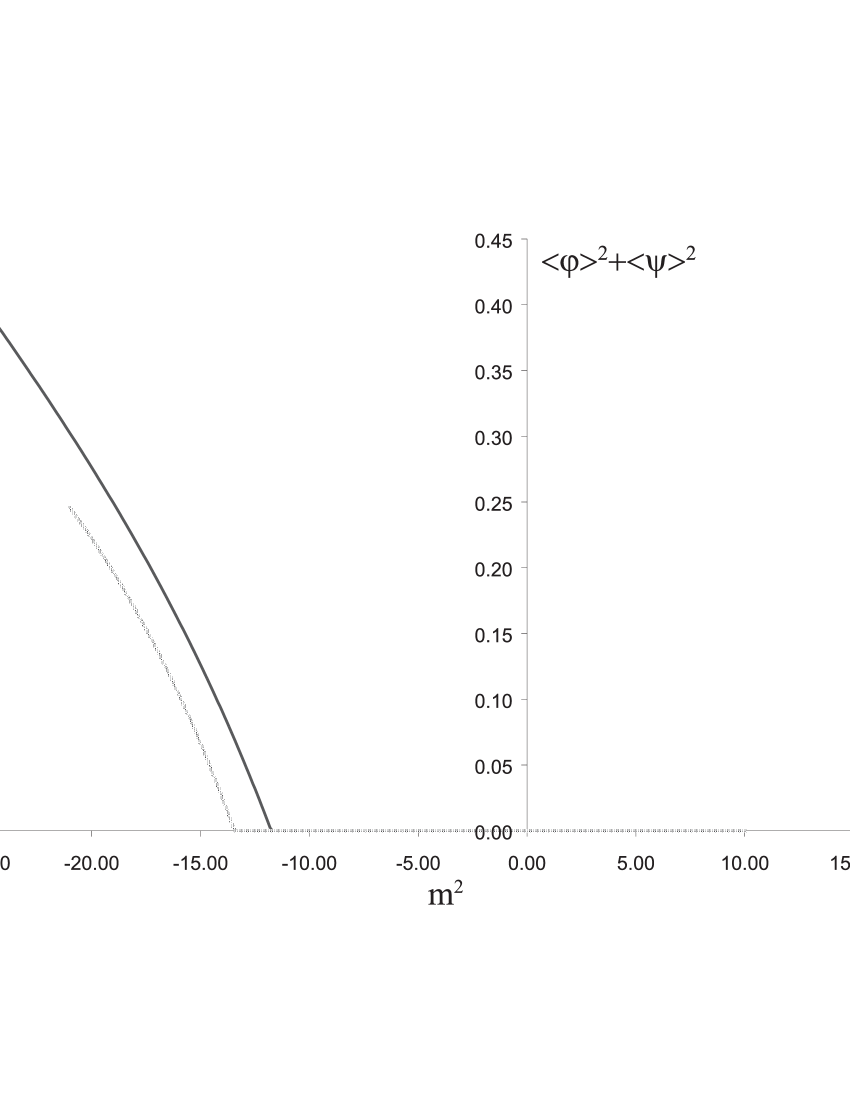
Figure 4: This plot shows the first and third order result of ${\langle{\phi}\rangle}^{2}+{\langle{\psi}\rangle}^{2}$ vs. $m^{2}$ for $\lambda=25$. The phase transition occurs around $m^{2}\approx-13.4$ for third order and $m^{2}\approx-11.8$ for first order.

We can clearly see that the curves are continuous but that there is a sudden change in slope at $m^{2}\approx-13.4$ for the third order expansion (and at $m^{2}\approx-11.8$ for the first order expansion). This indicates a second order phase transition. Since we are working on a lattice and have not taken the continuum limit, the mass parameter $m$ is not a physical mass so the fact that the phase transition does not occur at $m^{2}=0$ (as it would classically) is not surprising. In any case we are working a long way from the perturbative regime. The fluctuations about the minimum can be estimated from the difference $(\big{\langle}\phi^{2}\big{\rangle}-\big{\langle}\phi\big{\rangle}^{2})+(\big{\langle}\psi^{2}\big{\rangle}-\big{\langle}\psi\big{\rangle}^{2})$ and this is shown in figure 5. This peaks at the phase transition as expected.

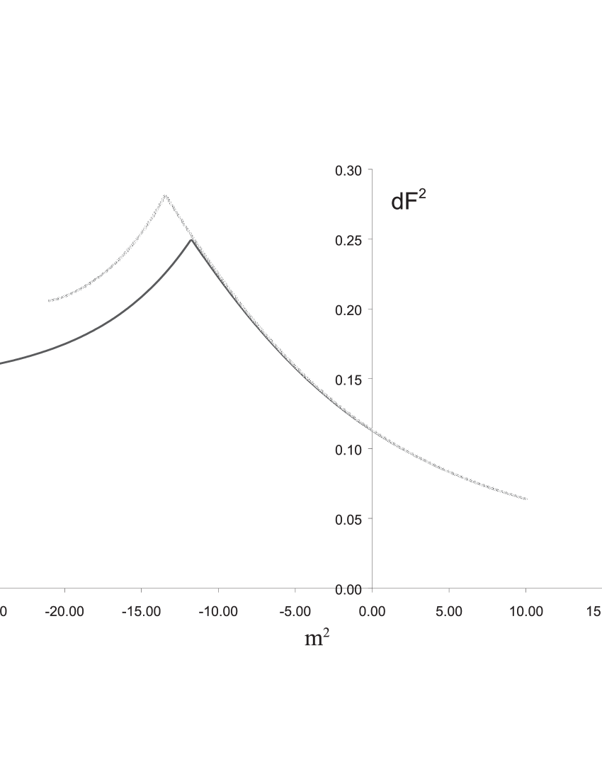
Figure 5: This plot shows the first and third order result of $dF^{2}:=({\langle{\phi^{2}}\rangle}-{\langle{\phi}\rangle}^{2})+({\langle{\psi^{2}}\rangle}-{\langle{\psi}\rangle}^{2})$ vs. $m^{2}$ for $\lambda=25$.

Another point to note is the way that non-zero results for $\big{\langle}\phi\big{\rangle}$ and $\big{\langle}\psi\big{\rangle}$ can be found in the OPE. This is a key difference between this method and lattice Monte Carlo methods. The OPE will always find one and only one vacuum solution even if there is more than one solution. It does this by allowing the sources $j$ to take non-zero values in which case the classical potential is tilted favouring one vacuum solution. This contrasts with lattice Monte Carlo methods which sample all possible vacuum states with equal likelihood. This means OPE methods are ideal for studying non-trivial field configurations, perhaps with defects present, by using classical sources to manipulate the effective quantum potential.

The last plot, figure 6, clearly shows the role of the O(2) symmetry in this method.

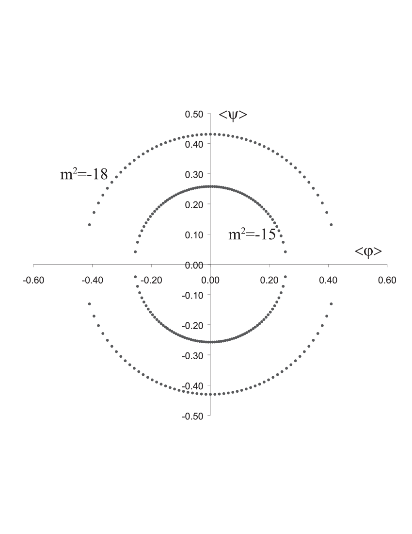
Figure 6: Plot of $\big{\langle}\psi\big{\rangle}$ vs. $\big{\langle}\phi\big{\rangle}$ for $m^{2}=-15.0$ and $m^{2}=-18.0$, for various initial values for the variational parameters. $\lambda=25.0$. We see that there are many degenerate vacuum states for a given $m^{2}$ in the broken symmetry regime.

The plot of $\big{\langle}\psi\big{\rangle}$ vs. $\big{\langle}\phi\big{\rangle}$ for $m^{2}=-15.0$ (inner curve) and $m^{2}=-18.0$ (outer curve) both show circles, i.e. the quantity $\big{\langle}\phi\big{\rangle}^{2}+\big{\langle}\psi\big{\rangle}^{2}$ is a constant.

It is important to note the form of the solutions found for the unphysical parameters $j_{\phi},j_{\psi},k_{+}$ and $k_{-}$. In the unbroken phase, $j_{\phi}=j_{\psi}=0$. In the broken phase while $|j|^{2}=j_{\phi}^{2}+j_{\psi}^{2}$ is a non-zero constant for a given set of physical parameters $m^{2}$ and $\lambda$, with a different solution for the $j$’s corresponding to each point on the circles in figure 6. This immediately suggests that $|j|$ acts as an order parameter. Thus a calculation of just the free energy, and by implication the variational parameters, rather than of any expectation value can be used find the location of the transition, as shown in figure (7).

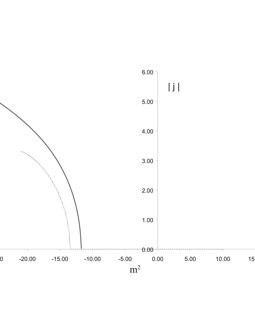
Figure 7: Plot of $|j|$ vs. $m^{2}$ for $\lambda=25.0$. It shows that this variational parameter acts as an order parameter.

The solution for $k_{+}$ was equal to $m^{2}$ in the unbroken regime and within 10% of $m^{2}$ otherwise, as shown in figure 8.

Figure 8: Plot of $(-1-k_{+}/m^{2})$ which minimise the third order free energy vs. $m^{2}$ for $\lambda=25.0$.

Thus $(K_{+}+m^{2})$ is acting as another order parameter. This shows that its numerical value, chosen by minimising the free energy, is keeping $S$ and $S_{0}$ as similar to each other as possible. However, it is not so much the numerical value of $k_{+}$ but the behaviour of functions as we vary $k_{+}$ which is important. As remarked above, there is often no minimum in the $k_{+}$ variable when there are minima in the other variational parameters.

Finally we note that that $k_{-}=0$ always minimised the free energy, within numerical accuracy. This latter result is of particular significance with regards the symmetry of our ansatz $S_{0}$, and we will now turn to consider this aspect.

To explain these results, in particular figure 6, we must consider the symmetry of the problem. $S$ is invariant under O(2) transformations such as

$$\vec{\phi}\rightarrow\vec{\phi}^{\prime}=U\vec{\phi},\;\;\;U=\left(\begin{array}[]{cc}\cos(\theta)&\sin(\theta)\\ -\sin(\theta)&\cos(\theta)\end{array}\right),\;\;\;\vec{\phi}=\left(\begin{array}[]{c}\phi\\ \psi\end{array}\right),\;\;\;$$ (13)

Our $S_{0}$ of (6) is not O(2) invariant if $k_{-}\neq 0$ or if the $j$ parameters are non-zero. However it is easy to see that

$$S_{0}(\vec{\phi};m^{2},\lambda;\vec{j},k_{+},k_{-}=0)=S_{0}(\vec{\phi}^{\prime}=U\vec{\phi};m^{2},\lambda;\vec{j}^{\prime}=U\vec{j},k_{+},k_{-}=0)$$ (14)

where $\vec{j}=(j_{\phi},j_{\psi})$. That is, there is a set of field independent transformations for $j_{\phi},j_{\psi}$ and $k_{+}$ which leave $S_{0}$ invariant under the O(2) field transformation. Note that we must have $k_{-}=0$ for this to be true, so let us for the moment assume that this value minimises the free energy.

Using this O(2) transformation we note that the integration measure is also O(2) invariant. It is then easy to show that at whatever order in $\delta$ we truncate our free energy expression, if the set $\{\tilde{\vec{j}},\tilde{k}_{+},\tilde{k}_{-}=0\}$ minimises the free energy then the set $\{\tilde{\vec{j}^{\prime}},\tilde{k}_{+},\tilde{k}_{-}=0\}$ also minimises the free energy. It then follows that a calculation of any O(2) invariant physical object will not depend on which solution for the variational parameters we use. In particular the free energy, $\big{\langle}\phi^{2}\big{\rangle}+\big{\langle}\psi^{2}\big{\rangle}$, and $\big{\langle}\phi\big{\rangle}^{2}+\big{\langle}\psi\big{\rangle}^{2}$ will all give results which are independent of the solution for the variational parameters. For objects like $\big{\langle}\phi\big{\rangle}$ which are not O(2) invariant, we can still relate one solution found for it, with a particular set of variational parameters, to another solution for $\big{\langle}\phi\big{\rangle}$ and another set of variational parameters. The relationship is precisely the simple O(2) transformations discussed here.

Plotting out final values for the variational parameters $j_{\phi}$ and $j_{\psi}$ for the different initial conditions used in producing figure (6) we found that $j_{\phi}$ and $j_{\psi}$ also form circles in a $j_{\phi}$-$j_{\psi}$ plane (for fixed $m^{2}$ and $\lambda$). Actually, there is a one-to-one correspondence between pairs of $j_{\phi}$, $j_{\psi}$ and $\big{\langle}\phi\big{\rangle}$, $\big{\langle}\psi\big{\rangle}$ – two points separated by a certain angle on the $j$ circle correspond to two points separated by the same angle on the expectation value circle; so to get one of the points from the circles in figure 6, we fix $j_{\phi}$ to a certain value, and minimize $F$ in the remaining $3$-dimensional parameter space. Once the point is found, we fix $j_{\phi}$ to a different value, and minimize again, thereby finding a different point. This is the explicit display that O(2) symmetry transforms both $j$’s and $\phi$’s with the same rotation matrix. The fact that we found $k_{+}$ was constant for all these solutions and that $k_{-}=0$ confirms the role of the symmetry transformations (13) and (14).

The presence of the variational parameter $k_{-}$, which does not respect the O(2) symmetry even if we allow field independent transformations, is a crucial distinction from the work of [26, 27] and [12]. It means that we have allowed our model to break the bounds of the symmetry of $S$ if the dynamics so choose. Thus one of the most important numerical results we have is that $k_{-}=0$ to numerical accuracy (at least six significant figures). Once this is known, only then do the symmetry arguments of the previous paragraph explain the circles of figure 6.

This explicit display of the role of the symmetry in the solutions suggests an interesting check, namely to impose the symmetry on the $S_{0}$. Thus, we ran the whole process again holding $k_{-}=0$, i.e. minimizing in a $3$-dimensional parameter space. We recovered the circle of $j$’s (at fixed $m^{2}$). We can then take it a stage further as in addition to holding the $k_{-}=0$, we can also fix one of the $j$’s to zero, and thus minimize in a $2$-dimensional parameter space. In the un-broken symmetry regime, the $j$’s are zero anyway, while in the broken symmetry phase there is an infinite set of equally valid solutions for the variational parameters, so holding one of the $j$’s at zero does not imply any loss of generality of the results.

In principle, one of the big advantages of the OPE is that one can systematically study higher orders through a straight forward extension of the method used here. However, it is likely that no solution for the variational parameters will be found at the next order, just as none was found at second order. As mentioned earlier, this behaviour is common in an OPE. Thus we would need to calculate $K_{5}$ or $L_{5}$..

To summarize, the OPE method used here works well in identifying the phase transition when there is a continuous symmetry, provided we fix the variational parameters by minimizing the free energy and we do not use the previously successful principle of minimal sensitivity. The explanation for the failure of the latter approach in this case after its earlier successes seems to be our use of a variational parameters which are quadratic in the Higgs fields. Another clear message coming from this work is that the optimal solutions choose a trial action $S_{0}$ which has the same symmetry as the full action $S$. This fact can be exploited to dramatically reduce the number of variational parameters used, which in turn will simplify and accelerate the analysis of more complicated models. Next, the source variational parameters, $j$, and the combination $(k_{+}+m^{2})$, act as order parameters. Thus one can identify the transition point from free energy calculations alone which is a further simplification when trying to find the phase diagram. We also note that this method can be used to study just one of many equivalent vacuum solutions which distinguishes it from lattice Monte Carlo. On the other hand, as shown here with just three orders, the OPE has a practical and systematic way of improving its accuracy, unlike other analytic non-perturbative methods. Thus we have demonstrated that OPE offers a practical route to the study of models with Higgs sectors and continuous symmetries in non-perturbative problems.

Appendix

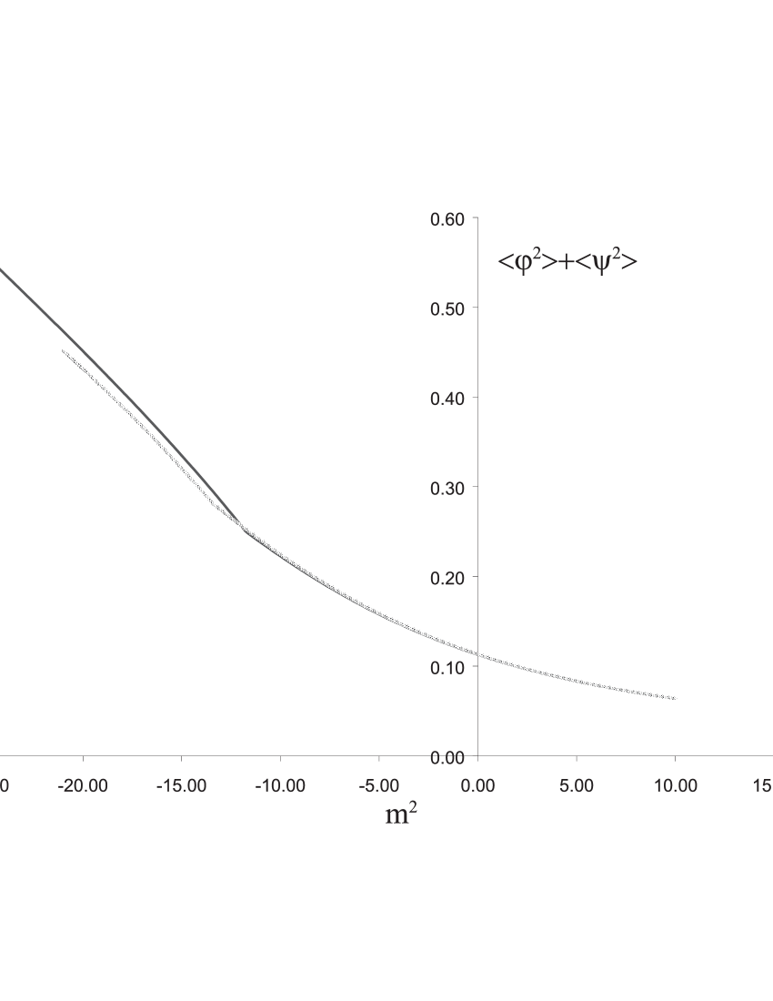
Figure 9: This plot shows the first and third order result of ${\langle{\phi^{2}}\rangle}+{\langle{\psi^{2}}\rangle}$ vs. $m^{2}$ for $\lambda=25$. It shows the phase transition, but the kink is not as clearly visible as in other plots.

References

- [1] R.J.Rivers, Path Integral Methods in Quantum Field Theory (Cambridge University Press, Cambridge, 1987).
- [2] I.Montvay, Nucl.Phys.B (Proc.Suppl.) 26 (1992) 57.
- [3] M.Lüscher, talk given at the 18th International Symposium on Lepton-Photon Interactions, Hamburg, 1997 [hep-ph/9711205].
- [4] M.Wortis, Linked Cluster Expansion, in “Phase Transitions and Critical Phenomena”, vol.3, eds. C.Domb and M.S.Green (Academic Press, London, 1974).
- [5] M.Lüscher and P.Weisz, Nucl.Phys.B 300 (1989) 325.
- [6] H.Meyer-Ortmanns and T.Reisz, Nucl.Phys.B (Proc.Suppl.) 73 (1999) 892 [hep-th/9809107].
- [7] H.F.Jones, Nucl.Phys.B (Proc.Suppl.) 39 (1995) 220.
- [8] W.Kerler and T.Metz, Phys.Rev.D 44 (1991) 1263.
- [9] A.Okapińska, Phys.Rev.D 35 (1987) 1835 [hep-th/9508087].
- [10] A.N.Sissakian, I.L.Solovtsov and O.P.Solovtsova, Phys.Lett.B 321 (1994) 381.
- [11] V.I.Yukalov, J.Math.Phys. 33 (1992) 3994.
- [12] C.M.Wu et al., Phase Structure of Lattice Theory by Variational Cumulant Expansion, Phys.Lett.B 216 (1989) 381.
- [13] I.R.C.Buckley, A.Duncan and H.F.Jones, Phys.Rev.D 47 (1993) 2554.
- [14] C.M.Bender, A.Duncan and H.F.Jones, Phys.Rev.D 49 (1994) 4219.
- [15] C.M.Bender, K.A.Milton, S.S.Pinsky and L.M.Simmons Jr., J.Math.Phys. 30 (1989) 1447.
- [16] W.E.Caswell, Ann.Phys. 123 (1979) 153.
- [17] J.Killingbeck, J.Phys.A 14 (1981) 1005.
- [18] A.Duncan and H.F.Jones, Phys.Rev.D 47 (1993) 2560.
- [19] J.O.Akeyo and H.F.Jones, Phys.Rev.D 47 (1993) 1668.
- [20] J.O.Akeyo and H.F.Jones, Z.Phys.C 58 (1993) 629.
- [21] J.O.Akeyo, H.F.Jones and C.S.Parker, Extended Variational Approach to the SU(2) Mass Gap on the Lattice, Phys.Rev.D 51 (1995) 1298 [hep-ph/9405311].
- [22] X.-T.Zheng, Z.G.Tan and J.Wang, Nucl.Phys.B 287 (1987) 171.
- [23] J.M.Yang, J.Phys.G 17 (1991) L143.
- [24] J.M.Yang, C.M.Wu and P.Y.Zhao, J.Phys.G 18 (1992) L1.
- [25] X.-T.Zheng, B.S.Liu, Intl.J.Mod.Phys.A 6 (1991) 103.
- [26] T.S. Evans, H.F. Jones and A. Ritz, An Analytical Approach to Lattice Gauge-Higgs Models, in “Strong and Electroweak Matter ’97”, ed. F.Csikor and Z.Fodor (World Scientific, Singapore, 1998, ISBN 981-02-3257-8) [hep-ph/9707539].
- [27] T.S. Evans, H.F. Jones and A. Ritz, On the Phase Structure of the 3D SU(2)-Higgs Model and the Electroweak Phase Transition, Nucl.Phys. B517 (1998) 599 [hep-ph/9710271].
- [28] P.M.Stevenson, Phys.Rev.D 23 (1981) 2916.