Abstract

By studying the non-linear effects of overlapping instanton pairs we address difficulties in the identification of instanton distributions when the average instanton size is comparable to the average distance. For the exact charge two solution, we study how its parametrisation relates to a description in terms of individual instantons. There exist two dual sets of parameters describing the same charge two instanton solution. This duality implies the existence of a minimal separation between two instantons. Conventionally used lattice instanton finder algorithms based on the assumption of diluteness tend to underestimate instanton sizes. Finally we numerically confirm this for realistic parameters of the instanton liquid. The effect is enhanced by parallel orientation in group space.

1 Introduction

In recent years the instanton liquid model has been very successful in describing the low energy properties of light hadrons [1]. On the other hand, it seems quite unlikely that instantons can account for confinement [2]. This is certainly the case if the instanton liquid is sufficiently dilute and the instanton size distribution falls off rapidly enough for large instantons. If the fall-off is slow, e.g. as $\rho^{-5}$ or $\rho^{-3}$, a linear term in the heavy quark potential due to instantons has been claimed [3], although these results are controversial. Still, a proper understanding of the tail of the instanton size distribution may have physical significance.

Unfortunately very little is known about it. Lattice simulations are typically done on too small volumes and have too poor statistics to contain any precise information on the tail of the distribution. Moreover, even the question of what non-perturbative mechanism suppresses large instantons is still unanswered, although some recent attempts have been made [4]. In this paper we would like to make some remarks on these issues by studying the most general charge two instanton solution. Our observations will be about the (possible mis)interpretations of the lattice data.

In lattice determinations [5, 6, 7] of the instanton liquid parameters one usually starts with the assumption that the liquid is dilute enough, i.e. the individual pseudoparticles are far enough apart that they do not distort one another considerably. Only then does the “instanton size” have an unambiguous meaning. Treating the $Q=2$ case exactly can be thought of as the next order approximation when one takes into account the distorting effect of like charge nearest neighbour pairs.

To fix the notation, we start with briefly summarising the ADHM construction [8] of the general $Q=2$ solution [9]. Then we discuss the ambiguities arising in the identification between the “physical” parameters and the ones appearing in the ADHM construction, giving rise to two dual descriptions of the same physical configuration. This duality maps large separation between the constituents to small separation [10] and depends non-trivially on the relative gauge orientation of the two instantons. It has two important consequences for the identification of instantons from the charge density profile, most clearly seen in the two extreme cases. Namely parallel and perpendicular relative gauge orientation (the SU(2) invariant angle being 0 and $\pi/2$ respectively). If the orientation is perpendicular, the two instantons cannot be closer to each other than a minimal distance $\sqrt{2\rho_{1}\rho_{2}}$ set by their sizes $\rho_{i}$. If the relative orientation is parallel and the two constituents have the same size $\rho$, when they get close to each other, the charge density looks like the super-imposition of a small instanton of size proportional to the separation, plus another instanton of size $\sqrt{2}\rho$ right under the small one. If the relative orientation and sizes are not fine tuned, some combination of the above effects will take place.

The first effect controls how close two instantons can get to each other. The second one can potentially hide large instantons from instanton finding algorithms based on the diluteness assumption and thereby it can significantly distort the instanton size distribution. In the last part of the paper we present quantitative data on how these effects are manifested in realistic lattice situations. This is done by generating the charge density of instanton pairs, as given by the exact $Q=2$ solutions, and comparing the size distribution thus prescribed by the original data with that found by lattice instanton finder algorithms. We observe that the results depend very strongly on the relative orientation in group space, yielding a strong suppression of large instantons for parallel orientation.

2 Physical Parameters for $Q=2$ Instantons

The fundamental objects describing the most general SU(2) charge $Q$ instanton solution in the ADHM construction are the $Q$-dimensional row vector $\lambda$ and the $Q\times Q$ symmetric matrix $B$, both having quaternionic elements [8]. (A quaternion $x$ can be parametrised with 4 real numbers as $x=x_{\mu}\sigma_{\mu}=x_{0}+ix_{k}\tau_{k}$, where $\tau_{k}$ are the Pauli matrices.) The ADHM data can be conveniently summarised in a single $Q\times(Q+1)$ quaternionic matrix $\Delta(x)$ which in the $Q=2$ case can be parametrised as

$$\Delta(x)=\left(\begin{array}[]{cc}\lambda_{1}&\lambda_{2}\\ y+z-x&u\\ u&y-z-x\end{array}\right).$$ (1)

$\Delta(x)$ describes a charge two self dual solution of the Yang-Mills equations if and only if the matrix $\Delta(x)$ satisfies the ADHM constraint that $\Delta^{\dagger}(x)\Delta(x)$ be real quaternionic (i.e. proportional to $\sigma_{0}$) and invertible. Here $\lambda_{1,2}$, $y$, $z$, and $u$ are quaternionic parameters, and $x=x_{\mu}\sigma_{\mu}$ denotes a space-time position. In terms of our parametrisation of the charge two case, the ADHM constraint reads as

$$\Lambda\equiv\frac{1}{2}\left(\lambda_{2}^{\dagger}\lambda_{1}\,-\,\lambda_{1}^{\dagger}\lambda_{2}\right)\;=\;z^{\dagger}u-u^{\dagger}z,$$ (2)

where the symbol $\Lambda$ is introduced to simplify the notation. This equation does not specify $u$ unambiguously; the most general solution can be written as [9]

$$u\;=\;\frac{z\Lambda}{2|z|^{2}}+\alpha z,$$ (3)

where $\alpha$ is an arbitrary real constant.

At this point it is instructive to compare this most general ADHM ansatz with the special case of the ’t Hooft ansatz [11] in order to identify the physical parameters. This special case is obtained for parallel gauge orientations, $\lambda_{1}=\rho_{1}\sigma_{0}$ and $\lambda_{2}=\rho_{2}\sigma_{0}$ real and $u=0$, which solves the ADHM constraint, eq. (2). We can identify $\rho_{1}$ and $\rho_{2}$ as the scale parameters (sizes), and $y\pm z$ as the locations of the two instantons. The action density of the solution, valid for all choices of parameters [12],

$$q(x)=-\partial_{\mu}^{2}\partial_{\nu}^{2}\log\det(\Delta^{\dagger}(x)\Delta(x))$$ (4)

indeed agrees in this case with the action density of the ’t Hooft solution.

The most general charge two ADHM solution can be described by the following set of free parameters: $\rho_{1,2}=|\lambda_{1,2}|$, the scale parameters; $\lambda_{1}^{\dagger}\lambda_{2}/(|\lambda_{1}||\lambda_{2}|)\in SU(2)$, the relative gauge orientation; and $y\pm z$ the location of the constituents. This gives a total number of 13 real parameters, in agreement with the general result that the charge $Q$ solution has $8Q-3$ parameters. For $Q=2$ the conformal generalisation of the ’t Hooft ansatz [11] also has 13 parameters, which can be related to the ADHM parametrisation [13].

The charge $Q$ ADHM ansatz is well known to have an $O(Q)$ symmetry acting on the parameters as

$$\lambda\rightarrow\lambda T^{-1},\;\;B\rightarrow TBT^{-1},\;\;T\in O(Q).$$ (5)

In the $Q=2$ case, using our parametrisation, the $SO(2)$ symmetry amounts to

$$\pmatrix{z\cr u}\rightarrow\pmatrix{\hphantom{-}\cos 2\psi&\sin 2\psi\cr-\sin 2\psi&\cos 2\psi}\pmatrix{z\cr u},\quad\pmatrix{\lambda_{1}\cr\lambda_{2}}\rightarrow\pmatrix{\hphantom{-}\cos\psi&\sin\psi\cr-\sin\psi&\cos\psi}\pmatrix{\lambda_{1}\cr\lambda_{2}},$$ (6)

while $y$ is left unchanged. The $Z_{2}$ transformation that extends this to the full $O(2)$ symmetry is generated by $T=\tau_{1}$, which interchanges $\lambda_{1}$ with $\lambda_{2}$ and changes the sign of $z$. Different sets of parameters related by this $O(2)$ symmetry describe the same physical solution [13]

$$A_{\mu}(x)=\frac{1}{2}(1-\lambda F(x)\lambda^{\dagger})^{-1}\partial_{\nu}\left(\lambda\sigma^{\dagger}_{[\mu}\sigma^{\vphantom{\dagger}}_{\nu]}F(x)\lambda^{\dagger}\right),\quad F^{-1}(x)\equiv\Delta^{\dagger}(x)\Delta(x),$$ (7)

where $\lambda=(\lambda_{1},\lambda_{2})$. At first sight this seems to imply that we have one less free parameter. This is, however, compensated by the fact that, in general, solutions to the ADHM constraint with different values of $\alpha$ (eq. (3)) result in physically different gauge field configurations, as one can easily be convinced of by computing $\det(\Delta^{\dagger}(x)\Delta(x))$.

Ideally one would like to fix this ambiguity together with the $O(2)$ symmetry to have a one-to-one correspondence between the gauge inequivalent solutions and the 13 parameters describing them. Our choice of these parameters, which we call “physical”, should be as close as possible to a superposition of two instantons. Looking at the situation of large separations ($|z|$ large), where the relative gauge orientation does not play a role, the action density should be the sum of two instantons of sizes $\rho_{1,2}$ located at $y\pm z$. This imposes $\alpha=0$, or equivalently $u_{\mu}z_{\mu}=0$. (The equivalence of the two conditions can be easily proved using eq. (2) and $a^{\dagger}b+b^{\dagger}a=2a_{\mu}b_{\mu}$ which holds for any two quaternions $a$ and $b$.) Choosing this particular solution to the constraint ensures that when the orientation of the constituents is parallel, the ADHM solution coincides with the ’t Hooft ansatz.

With this convention the identification of the “physical” parameters becomes almost unique. The prescription is that from each $O(2)$ orbit we have to choose the point that satisfies $u_{\mu}z_{\mu}=0$. Generally there are 16 such points on an $O(2)$ orbit describing the same gauge field configuration, as has been noted before [10]. They are generated by rotations (see eq. (6)) over multiples of $\pi/4$ and the $Z_{2}$ transformation, $\lambda_{1}\leftrightarrow\lambda_{2}$, $z\rightarrow-z$. Most of these do not affect the “physical” interpretation. But one ambiguity remains for which we choose the representative described by the $Z_{2}$ symmetry ($T=\tau_{1}$) combined with the rotation over $\psi=\pi/4$, providing the relation

$$\left(y,\,z,\,\lambda_{1},\,\lambda_{2},\,u=\frac{z\Lambda}{2|z|^{2}}\right)\;\;\longrightarrow\;\;\left(y,\,u,\,\frac{\lambda_{1}+\lambda_{2}}{\sqrt{2}},\,\frac{\lambda_{1}-\lambda_{2}}{\sqrt{2}},\,z\right).$$ (8)

We note that if the distance of the two instantons is $2|z|$ in one description, it is proportional to $1/|z|$ in the “dual” description, as long as the relative gauge orientation is not parallel ($\Lambda\neq 0$). Going beyond the issue of finding a unique parametrisation, the question now arises which of these two descriptions is the “physical” one. To answer this it is instructive to look at the charge density profile of a set of solutions with varying separations, keeping the other parameters fixed.

In Fig. 1 we show such a sequence.

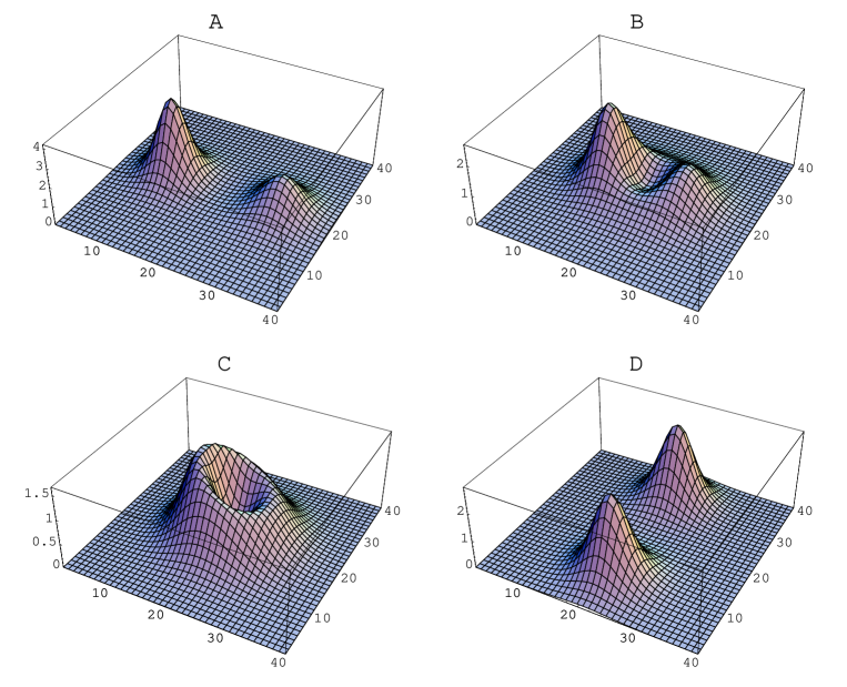
Figure 1: A pair of size $\rho_{1}=6.6$ and $\rho_{2}=8.3$ instantons with perpendicular relative gauge orientations. The centres are separated along the $x_{0}$ axis, the separation, $2|z|$ is 20.0 (A), 13.3 (B), 10.5 (C), and 5.0 (D). The action density is shown in the (01) plane.

The parametrisation listed is in terms of the l.h.s. of eq. (8). The scale parameters and relative orientation are described by $\lambda_{1}=6.6\sigma_{0}$, $\lambda_{2}=8.3\sigma_{1}$, and the separation between the constituents is always along the 0-axis. When they are far apart (A), corresponding to $2|z|=20.0$, the solution indeed looks like a pair of instantons along the 0-axis. As the separation decreases the two lumps merge together into an asymmetric ring (B-C) ($2|z|=13.3$ and 10.5 respectively). For even smaller separation: $2|z|=5.0$, (D) in the figure, the two lumps separate again but now displaced along the 1-axis. Clearly, our parametrisation is not “physical” any more at this stage; instead of two very close lumps separated along the 0-axis, we see two lumps farther apart but along the perpendicular 1-axis. On the other hand, we also have the dual parametrisation (r.h.s. of eq. (8)) at our disposal. Indeed, a short computation shows that in the dual description of (D) we have two instantons of the same scale parameter $\rho=7.5$ separated along the 1-axis at a distance of 22, evidently the correct “physical” description.

The general picture emerging from this exercise is quite clear. When $|z|$ is large, more precisely $|z|^{2}\gg|\Lambda|$, the original description is “physical”, i.e. describing two superposed instantons separated by a distance $2|z|$. When $|z|$ is small, however, the dual description is the more “physical” one. There is an intermediate region where the solution cannot be approximated by a combination of two instantons, here the question which parameter set to use for the physical description is ill defined.

In the rest of this Section we discuss two simple consequences of this dual choice of parametrisation. The first one is that two instantons, as identified from maxima in the action density, can never get closer to each other than a minimal distance

$$2|z|_{min}=\sqrt{2\rho_{1}\rho_{2}\sin\phi},$$ (9)

where $\phi$ is the invariant angle of the relative group orientation. $|z|_{min}$ is defined by the property that the two dual descriptions have the same separation $2|z|_{min}$ between the constituents. If $|z|$ is chosen to be smaller than this, the two instantons “scatter off” in the $z\Lambda$ direction and one has to switch to the dual description. It is also interesting to observe the very special case when $\rho_{1}=\rho_{2}=\rho$ and $\phi=\pi/2$. In this case, $2|z|_{min}=\sqrt{2}\rho$ gives a self-dual point where the two parametrisations completely coincide and the charge density has an axial symmetry in the $(z\Lambda,z)$ plane. For these parameters the density profile is ring-like, not unlike the case of monopoles [14], but apparently not noted before for instantons. In particular, the solution does not degenerate to one with topological charge $Q=1$, as conjectured in ref. [10]. This only happens in the case of parallel gauge orientation, for $\rho_{1}=\rho_{2}$ and $z=0$ (see eq. (10) below).

The discussion so far applies only to the $\Lambda\neq 0$ case. Moreover, if $\phi\approx 0$, then the switching between the two parametrisations occurs at very small $|z|$ (see eq. (9)) and other interesting effects might come into play when the two constituents are very close. Let us now look at the extreme situation when $\phi=0$, the relative orientation is parallel and consequently $\Lambda=0$. In this case the two parametrisations are

$$\left(y,\,z,\,\rho_{1}\sigma_{0},\,\rho_{2}\sigma_{0},\,0\right)\;\;\longrightarrow\;\;\left(y,\,0,\,\frac{\rho_{1}+\rho_{2}}{\sqrt{2}}\sigma_{0},\,\frac{\rho_{1}-\rho_{2}}{\sqrt{2}}\sigma_{0},\,z\right).$$ (10)

In the limit $z\rightarrow 0$ the two descriptions become equivalent, there is no way to choose between them. One can see that two instantons of scale parameters $\rho_{1,2}$ ($\rho_{1}\sim\rho_{2}$) on top of each other is equivalent to a small instanton of size $|\rho_{2}-\rho_{1}|/\sqrt{2}$ on top of a larger one of size $(\rho_{2}+\rho_{1})/\sqrt{2}$. In this extreme case any lattice instanton finder based on the diluteness assumption would find only the former smaller instanton and nothing else. Moreover due to the strongly non-linear character of the Yang-Mills equations, when two instantons come close with parallel orientation, both peaks become narrower and sharper and are thus identified by any lattice algorithm as “small” instantons. At best one misses one large instanton in the background; at worst one misinterprets two large instantons as two small ones. The effect is similar at $\phi\approx 0$ and can provide a mechanism to hide large instantons as some smooth background that remains unnoticed by lattice instanton finder algorithms.

3 The Instanton Size Distribution

We have seen how the identification of single instanton parameters becomes ambiguous when instantons overlap. We discussed what happens in the two extreme cases of parallel and perpendicular orientation in group space. In between, some combination of the two above described effects takes place. We expect that the exact way this affects the instanton size distributions measured on the lattice will depend on the relative orientation of nearest neighbour pairs.

Figure 2: The instanton size distribution with the relative orientation being distributed according to the Haar measure. The solid line indicates the distribution of the “physical” (see text) ADHM size parameter, the dotted and the dashed lines are the size distributions determined by the instanton finder algorithms of Ref. [6] and [7] respectively.

In the remainder of the paper we study numerically how the relative orientation can affect the lattice instanton size distribution. In order to see the trends as clearly as possible, instead of trying to mimic the “real” distribution of relative orientations, we use two simple orientation distributions: the Haar measure, and all instantons taken parallel. Due to the $\sin^{2}\!\phi$ factor, the Haar measure very strongly favours (close to) perpendicular orientation, thus our two distributions almost represent the two possible extremes. We generated the charge density of a set of instanton pairs with the ADHM construction using eq. (4). The parameters of the ADHM ansatz were taken as follows. The instanton scale parameters $(\rho_{1,2})$ were distributed independently and qualitatively similar to that found on the lattice, except for an enhanced tail (for $\rho$ large). We artificially enhanced the tail of the distribution in order to test whether such a tail can remain undetected by the lattice instanton finders. The separation $2|z|$ was Gaussian distributed with mean 7.0, and variance of 1.0.

The resulting charge densities — each pair resolved on a $16^{4}$ grid — were then analysed using two different instanton finder algorithms [6, 7]. The details of these algorithms are not relevant in the present context. However their most important common feature is that they are both based on the dilute gas assumption. They identify the highest peaks in the charge density and estimate the instanton sizes from the fall-off of the density in the vicinity of the maximum.

Figure 3: The same as Fig. 2, except the relative orientation in group space is always chosen parallel.

In Fig. 2 we show the instanton size distributions found by the algorithms of Refs. [6] (dotted line) and [7] (dashed line) along with the distribution of the ADHM size parameters used to construct the charge densities (solid line), representing the physical choice of parameters. The Haar measure was used for the gauge orientation. One of the instanton finders seems to somewhat suppress the enhanced tail while this effect is not significant with the other.

In Fig. 3 we plotted the size distributions obtained when all the pairs were taken parallely oriented in group space. All the conventions are the same as in Fig. 2. Here the two instanton finders both yield a significantly suppressed tail.

We also considered ensembles (not shown) which in terms of the relative orientation are in between the two shown. We can draw the following general conclusion. The two instanton finders display the same trend; the more parallel the pair is in group space the more suppressed the large instantons become. This is partly due to the effect that large instantons can “hide” under small ones that produce sharper peaks in the charge density. The other effect is that, when two instantons come close with approximately parallel orientation, they look narrower and are thus interpreted by the lattice algorithm as “small” instantons

4 Conclusions

To summarise, we studied the question of what happens when the instanton liquid is not dilute enough to be considered as a collection of individual pseudoparticles. The next approximation is to treat nearest pairs of like charge exactly. We established a correspondence between the parameters of individual instantons and the parameters of the charge two ADHM construction. After fixing most of the ambiguities of this correspondence we still have two dual sets of parameters describing the same charge two instanton solution. This duality turned out to imply the existence of a minimal distance between the two instantons, which is maximal in the case of perpendicular orientation. In the other extreme case of (nearly) parallel orientation, we found that instanton finders based on the diluteness assumption can have a tendency to miss large instantons or to underestimate instanton sizes. We numerically confirmed that this indeed happens for realistic parameters of the instanton liquid and the effect becomes larger for orientations closer to being parallel. In fact, a recent lattice study indicates that like charge pairs strongly favour parallel orientation compared to the Haar measure [15], therefore the effect we found can be potentially important.

References

- [1] T. Schäfer, and E.V. Shuryak, Rev. Mod. Phys. 70 (1998) 323.
- [2] D.I. Diakonov, V.Yu. Petrov, and P.V. Pobylitsa, Phys. Lett. B226 (1989) 372; T. DeGrand, A. Hasenfratz, and T.G. Kovács, Phys. Lett. B420 (1998) 97.
- [3] D. Diakonov and V. Petrov, “Confinement from Instantons?”, in: Non-perturbative approaches to Quantum Chromodynamics, Proceedings of the ECT∗ workshop, Trento, July 10-29, 1995, ed. D. Diakonov, Gatchina, 1995, p. 239; M. Fukushima, H. Suganuma, and H. Toki, Phys. Rev. D60 (1999) 094504; R.C. Brower, D. Chen, J.W. Negele, and E. Shuryak, Nucl. Phys. B (Proc. Suppl.) 73 (1999) 512.
- [4] E.V. Shuryak, “Probing the boundary of the nonperturbative QCD by small size instantons”, hep-ph/9909458.
- [5] C. Michael, and P.S. Spencer, Phys. Rev. D52 (1995) 4691; D.A. Smith, and M.J. Teper, Phys. Rev. D58 (1998) 014505.
- [6] Ph. de Forcrand, M. García Pérez, and I.-O. Stamatescu, Nucl. Phys. B499 (1997) 409.
- [7] T. DeGrand, A. Hasenfratz, and T.G. Kovács, Nucl. Phys. B505 (1997) 417.
- [8] M.F. Atiyah, N.J. Hitchin, V.G. Drinfeld, and Yu.I. Manin, Phys. Lett. A65 (1978) 185.
- [9] N.H. Christ, E.J. Weinberg, and N.K. Stanton, Phys. Rev. D18 (1978) 2013.
- [10] N. Dorey, V.V. Khoze, and M.P. Mattis, Phys. Rev. D54 (1996) 2921 (Appendix D).
- [11] G. ’t Hooft, as quoted in R. Jackiw, C. Nohl, and C. Rebbi, Phys. Rev. D15 (1977) 1642.
- [12] H. Osborn, Nucl. Phys. B159 (1979) 497.
- [13] E.F. Corrigan, D.B. Fairlie, S. Templeton, and P. Goddard, Nucl. Phys. B140 (1978) 31.
- [14] P. Forgács, Z. Horváth and L. Palla, Nucl. Phys. B192 (1981) 141; M.F. Atiyah, and N.J. Hitchin, The Geometry and Dynamics of Magnetic Monopoles, Princeton Univ. Press 1988.
- [15] E.M. Ilgenfritz, and S. Thurner, “Correlated instanton orientations in the SU(2) Yang-Mills vacuum and pair formation in the deconfined phase”, hep-lat/9810010.