PM/99–51

I summarise the virtual effects of the new particles predicted by supersymmetric extensions of the Standard Model on the high–precision electroweak observables measured at LEP/SLC, the Tevatron and CLEO. I will then discuss in some details the two–loop SUSY–QCD corrections to the $\rho$ parameter.

Lecture givent at X Escola Jorge André Swieca de Partículas e Campos

7–12 February 1999, Aguas de Lindõia, São Paulo, Brazil.

SUPERSYMMETRY EFFECTS ON HIGH–PRECISION
ELECTROWEAK OBSERVABLES

I summarise the virtual effects of the new particles predicted by supersymmetric extensions of the Standard Model on the high–precision electroweak observables measured at LEP/SLC, the Tevatron and CLEO. I will then discuss in some details the two–loop SUSY–QCD corrections to the $\rho$ parameter.

1 Introduction/Motivations:

Supersymmetry (SUSY) is the most attractive extension of the Standard Model (SM) $\!{}^{{\bf?},{\bf?},{\bf?}}$. It not only stabilizes the huge hierarchy between the weak and GUT scales against radiative corrections, but also if SUSY is broken at a sufficiently high scale, it allows us to understand the origin of the hierarchy in terms of radiative gauge symmetry breaking. Moreover, SUSY models offer a natural solution to the dark matter problem and allow for a consistent unification of the all known gauge couplings. Many new particles are predicted in these theories; the search for these states and the study of their properties, is and will be, one of the major goals of present and future colliders.

A wide range of searches for supersymmetric particles are performed at present colliders, in particular at LEP and the Tevatron, and no direct signal beyond the SM expectation was observed yet, unfortunately. Therefore new limits on the masses of these particles, assuming different models, are set by the various experiments; see for instance Refs. $\!{}^{{\bf?},{\bf?}}$. Most of the experimental limits at LEP2 are close to the kinematical thresholds $\!{}^{{\bf?}}$, and the discovery of SUSY particles has to await for the upgraded Tevatron $\!{}^{{\bf?}}$, the LHC $\!{}^{{\bf?}}$ or for a future $e^{+}e^{-}$ linear collider $\!{}^{{\bf?}}$.

However, rather than waiting for these future experiments, one could use the enormous amount of electroweak precision data on $Z$ and $W$ bosons, collected at the $e^{+}e^{-}$ colliders LEP and the SLC, and at the Tevatron $\!{}^{{\bf?},{\bf?},{\bf?}}$. These high–precision measurements provide a unique tool in the search for indirect effects of new particles, and in particular SUSY particles, through possible small deviations of the experimental results from the theoretical predictions of the minimal SM. This is what I will try to summarize in this Lecture.

In section 2, I will briefly describe the Minimal Supersymmetric extension of the Standard Model (MSSM), summarise the experimental limits on the SUSY particle masses and the high–precision measurement of the electroweak observables. In section 3, I will discuss the observables where potentially large effects form SUSY particles could be expected: the $Z$ boson decay widths into hadrons, the $W/Z$ boson self–energies and the radiative decay $b\to s\gamma$. In section 4, I will focuss on the $\rho$ parameter, and show an exemple of a calculation of SUSY–QCD corrections at the two–loop level, highlightening the new features compared to SM calculations.

2 Physical Set–Up

2.1 The Minimal Supersymmetric Standard Model

The MSSM is the most economical low–energy supersymmetric extension of the SM. The unconstrained model is defined by the following four basic assumptions [for more details, see the reviews in Ref. $\!{}^{{\bf?},{\bf?}}$]:

– It is based on the SM gauge symmetry ${\rm SU(3)_{C}\times SU(2)_{L}\times U(1)_{Y}}$. SUSY implies then, that the spin–1 gauge bosons, and their spin–1/2 superpartners the gauginos [bino $\tilde{B}$, winos $\tilde{W}_{1-3}$ and gluinos $\tilde{g}_{1-8}$] are in vector supermultiplets.

– There are only three generations of spin–1/2 quarks and leptons [no right–handed neutrino] as in the SM. The left– and right–handed chiral fields belong to chiral superfields together with their spin–0 SUSY partners the squarks and sleptons. In addition, two chiral superfields with respective hypercharges $-1$ and $+1$ for the cancellation of chiral anomalies, are needed. Their scalar components give separately masses to the isospin +1/2 and $-$1/2 fermions. Their spin–1/2 superpartners, the higgsinos, will mix with the winos and the bino, to give the mass eigenstates, the charginos $\chi_{1,2}^{\pm}$ and neutralinos $\chi^{0}_{1,2,3,4}$.

– To enforce lepton and baryon number conservation, a discrete and multiplicative symmetry called R–parity is imposed. The R–parity quantum numbers are $R=+1$ for the ordinary particles and $R=-1$ for their supersymmetric partners. The conservation of $R$–parity has important consequences: the SUSY particles are always produced in pairs, in their decay products there is always an odd number of SUSY particles, and the lightest SUSY particle (LSP) is absolutely stable.

These conditions are sufficient to completely determine a globally SUSY Lagrangian. The kinetic part is obtained by generalizing the notion of covariant derivative to the SUSY case, and one then has to add the most general superpotential compatible with gauge invariance, renormalizability and R–parity.

To break SUSY, while preventing the reappearance of the quadratic divergences, one adds to the previous Lagrangian a set of terms which explicitly but softly breaks SUSY: mass terms for the gluinos, winos and binos; mass terms for the scalar fermions; mass and bilinear terms for the Higgs bosons; and trilinear couplings between sfermions and Higgs bosons.

This unconstrained MSSM, for generic values of the parameters, might lead to severe phenomenological problems, such as flavor changing neutral currents (FCNC), unacceptable amount of additional CP–violation, color and charge breaking minima, etc… Furthermore, it contains a huge number of free parameters, which are mainly coming from the scalar potential: if we allow for intergenerational mixing and complex phases, 105 unknown parameters are introduced in addition to the 19 parameters of the SM! This feature of course will make any phenomenological analysis a daunting task. There are, fortunately, several phenomenological constraints which make some assumptions reasonably justified to constrain the model. Assuming that there are: no new source of CP–violation, no FCNC first and second generation sfermion universality will lead to 19 new input parameters only. Such a model, with this relatively moderate number of parameters [especially that, in general, only a small subset appears when one looks at a given sector of the model] has much more predictability and is much easier to be discussed phenomenologically.

All the phenomenological problems of the unconstrained MSSM discussed previously are solved at once if one assumes that the MSSM parameters obey a set of boundary conditions at the Unification scale. These assumptions are natural in scenarii where the SUSY–breaking occurs in a hidden sector which communicates with the visible sector only through gravitational interactions. These unification and universality hypotheses are as follows: unification of the gaugino masses $m_{1/2}$; universal scalar [sfermion and Higgs boson] masses $m_{0}$; universal trilinear couplings $A_{0}$. Besides these three parameters, the SUSY sector is described at the GUT scale by the bilinear coupling $B$ and the higgsino mass parameter $\mu$. However, one has to require that electroweak symmetry breaking takes place. This results in two minimization conditions of the Higgs potential and the equations can be solved for $B$ and $|\mu|$. Therefore, in this model, we will have only four continuous and one discrete free parameters: $\tan\beta$ [the ratio of the vev’s of the two–Higgs doublet fields], $m_{1/2},m_{0},A_{0}$ and ${\rm sign}(\mu)$. This model, usually referred to as the minimal Supergravity model or mSUGRA, is clearly appealing and suitable for thorough phenomenological and experimental scrutinity.

2.2 Lower limits on SUSY particle masses

The searches for SUSY particles at LEP concern sleptons, stops, sbottoms, charginos and neutralinos. These various particles decay to SM particles and two LSPs; therefore, SUSY signatures consist of some combination of jets or/and leptons and missing energy since the LSP escapes detection. The signal topology and the background conditions are in practice affected by the SUSY particle and the LSP mass difference ($\Delta M=m_{\rm SUSY}-m_{\chi^{0}_{1}})$ which controls the visible energy. Since all the background sources are due to well calculable processes with reasonable production cross sections compared to the signal, most of the decay channels are studied at LEP2. Another important key domain concerns the searches for the MSSM Higgs bosons. Presently, only the lighter neutral Higgs bosons $h$ and $A$ can be discovered at LEP2, since the CP–even Higgs boson $H$ and the charged Higgs bosons $H^{\pm}$ are expected to be too heavy. Each experiment (ALEPH, DELPHI, L3, OPAL) has accumulated data $\sim 55\;\rm pb^{-1}$ at $\sqrt{s}=183$ GeV in 1997. In october 1998, an amount of $150\;\rm pb^{-1}$ at $\sqrt{s}=189$ GeV is already recorded by each experiment, but the results including all the statistics for 1998 are not yet available.

At the Tevatron the main sources for SUSY are squarks and gluinos, abundantly produced due to the color factors and the strong coupling constant. Squarks or gluinos are produced in pairs, and decay directly or via cascades to at least two LSP’s. The classical searches rely on large missing transverse energy caused by the escaping LSPs. In addition, charginos and neutralinos are searched for via their leptonic decay channels by the two Tevatron experiments CDF and D0. Finally, searches for the MSSM charged Higgs boson are performed, and bounds on its mass have been set by both experiments. Each experiment has collected an integrated luminosity of about 110 pb^-1 at $\sqrt{s}=1.8$ TeV.

Since no evidence for production of supersymmetric particles has been found at LEP or the Tevatron, experimental limits on their production cross sections and masses has been derived. The mass limits are summarised in Table 1 from Ref. $\!{}^{{\bf?}}$.

Particle	Assumptions	Limit	Exp. source
h	$\tan\beta\geq$0.8	78.8	LEP2 Comb.
A	$\tan\beta\geq$0.8	79.1	LEP2 Comb.
H±	Br($\rm H\rightarrow c\bar{s})$ + Br($\rm H\rightarrow c\bar{s}$)=1	68	LEP2 Comb.
$\tilde{e}_{R}$	Br($\tilde{e}_{R}$ $\rightarrow e\chi_{1}^{0}$)=1, $\Delta$M$\geq 20~{}\rm GeV$	85	LEP2 Comb.
$\rm\tilde{\mu}_{R}$	BR($\rm\tilde{\mu}_{R}$ $\rightarrow\mu\chi_{1}^{0}$ )=1, $\Delta$ M $\geq$ 20 $\rm GeV$	71	LEP2 Comb.
$\rm\tilde{\tau}_{R}$	BR($\rm\tilde{\tau}_{R}$ $\rightarrow\tau\chi_{1}^{0}$)=1, $\Delta$ M $\geq 20~{}\rm GeV$	75	LEP2 Comb.
$\tilde{\nu}$		43	LEP1 $\Gamma_{Z}$
$\rm\tilde{t}_{1}$	BR($\rm\tilde{t}_{1}$ $\rightarrow c\chi_{1}^{0}$)=1, $\Delta$ M $\geq$ 15 $\rm GeV$	83	LEP2 Comb.
	BR($\rm\tilde{t}_{1}$ $\rightarrow c\chi_{1}^{0}$ )=1, ${\rm LEP2;~{}m_{\chi_{1}^{0}}\leq 50~{}GeV}$	122	CDF
$\rm\tilde{b}_{1}$	BR($\rm\tilde{b}_{1}$ $\rightarrow b\chi_{1}^{0}$ )=1, $\Delta$ M $\geq 15~{}\rm GeV$	75	LEP2 Comb.
$\rm\tilde{q}$	$\rm m_{\tilde{q}}\geq m_{\tilde{g}}$	216	CDF
	$\rm m_{\tilde{q}}\geq m_{\tilde{g}}$	260	D0
$\rm\tilde{g}$	$\mu\leq-100$ or $\mu\geq 200~{}\rm GeV$	173	CDF
	$\mu\leq-100$ or $\mu\geq 200~{}\rm GeV$	187	D0
$\chi^{\pm}_{1}$	Higgsino $\Delta$M $\geq 3~{}\rm GeV$	63	LEP2 Comb.
	Gaugino $\rm m_{0}$ $\geq 200~{}\rm GeV$	94.3	LEP2∗
$\chi^{0}_{1}$	Large $\rm m_{0}$	32.5	LEP2∗

Table 1: Summary of lower mass limits obtained at the Tevatron and at LEP2 up to $\sqrt{s}$ = 183, 189 GeV [^∗ at which just a small fraction of data has been used]; From Ref. [4].

2.3 High–precision data

The $e^{+}e^{-}$ colliders LEP and the SLC, in operation since 1989, have collected an enormous amount of electroweak precision data on $Z$ and $W$ bosons. Measurements at the $Z$–pole of $Z$ boson partial and total decay widths, polarisation and forward–backward asymmetries where made at the amazingly high accuracy of the level of one percent to one per mille; see Table 2 from Ref. $\!{}^{{\bf?}}$. The $W$ boson properties have in parallel been determined at the $p\bar{p}$ collider Tevatron with a constant increase in accuracy. The ongoing experiments at LEP2 and the near-future Tevatron upgrade will also, in the coming years, provide us with further increase in precision, in particular on the mass of the $W$ and the SLC might continue to improve the impressive accuracy already obtained in the electroweak mixing angle.

Another measurement of interest here, is the branching ratio for the radiative flavor changing decay $B\to X_{s}\gamma$ performed at LEP1 and by the CLEO collaboration. The most precise value and the SM expectation for the branching ratio are $\!{}^{{\bf?}}$:

$${\rm BR}(B\to X_{s}\gamma)\times 10^{4}=[3.14\pm 0.48]_{\rm exp}\ \ {\rm and}\ \ [3.29\pm 0.33]_{\rm th}$$

The availability of both highly accurate measurements and theoretical predictions, at the level of 0.1% precision and better, provides tests of the quantum structure of the SM, thereby probing its still untested scalar sector, and simultaneously accesses alternative scenarios such as the supersymmetric extension of the SM. Indeed, the lack of direct signals from new physics beyond then makes the high-precision experiments a unique tool also in the search for indirect effects, through possible small deviations of the experimental results from the theoretical predictions of the minimal SM.

Table 2: Precision observables: experimental results from combined LEP and SLD data for $Z$ observables and combined $p\bar{p}$ and LEP data for $M_{W}$, with the SM predictions; From Ref. [11].

Observable	Exper. value	SM best fit
$M_{Z}$ (GeV)	$91.1867\pm 0.0019$	91.1865
$\Gamma_{Z}$ (GeV)	$2.4939\pm 0.0024$	2.4956
$\sigma_{0}^{had}$ (nb)	$41.491\pm 0.058$	41.476
$R_{had}$	$20.765\pm 0.026$	20.745
$R_{b}$	$0.21656\pm 0.00074$	0.2159
$R_{c}$	$0.1732\pm 0.0048$	0.1722
$A_{FB}^{\ell}$	$0.01683\pm 0.00096$	0.0162
$A_{FB}^{b}$	$0.0990\pm 0.0021$	0.1029
$A_{FB}^{c}$	$0.0709\pm 0.0044$	0.0735
$A_{b}$	$0.867\pm 0.035$	0.9347
$A_{c}$	$0.647\pm 0.040$	0.6678
$\Delta\rho$	$1.0041\pm 0.0012$	1.0051
$\sin^{2}\theta_{W}$	$0.23157\pm 0.00018$	0.23155
$M_{W}$ (GeV)	$80.39\pm 0.06$	80.372

3 Potentially large virtual SUSY effects

3.1 The $\rho$ parameter

A possible SUSY signal might come from the contribution of the SUSY particle loops to the electroweak gauge–boson self–energies $\!{}^{{\bf?},{\bf?}}$: if there is a large splitting between the masses of these particles, the contribution will grow with the mass of the heaviest particle and can be sizable. This is similar to the SM case, where the top/bottom weak isodoublet generates a quantum correction that grows as $m_{t}^{2}$. This contribution enters the electroweak observables via the $\rho$ parameter $\!{}^{{\bf?}}$, which measures the relative strength of the neutral to charged current processes at zero momentum–transfer. It is mainly from this contribution that the top–quark mass has been successfully predicted from the measurement of $\sin^{2}\theta_{W}$ and $M_{W}$, a triumph for the electroweak theory.

The $\rho$ parameter, in terms of the transverse parts of the $W$– and $Z$–boson self–energies at zero momentum–transfer, is given by

$$\rho=(1-\Delta\rho)^{-1}\ ;\ \Delta\rho=\Pi_{ZZ}(0)/M_{Z}^{2}-\Pi_{WW}(0)/M_{W}^{2}$$ (1)

In the SM, the contribution of a fermion isodoublet $(u,d)$ to $\Delta\rho$ reads at one–loop:

$$\Delta\rho_{0}^{\rm SM}=\frac{N_{c}G_{F}}{8\sqrt{2}\pi^{2}}F_{0}\left(m_{u}^{2},m_{d}^{2}\right)\ ,F_{0}(x,y)=x+y-\frac{2xy}{x-y}\log\frac{x}{y}$$ (2)

The function $F_{0}$ vanishes if the $u$– and $d$–type quarks are degenerate in mass: $F_{0}(m_{q}^{2},m_{q}^{2})=0$; in the limit of large quark mass splitting it becomes proportional to the heavy quark mass squared: $F_{0}(m_{q}^{2},0)=m_{q}^{2}$. Therefore, in the SM the only relevant contribution is due to the top/bottom weak isodoublet. Because $m_{t}\gg m_{b}$, one obtains $\Delta\rho^{\rm SM}_{0}=3G_{F}m_{t}^{2}/(8\sqrt{2}\pi^{2})$, a large contribution which allowed for the prediction of $m_{t}$. However, in order that the predicted value agrees with the experimental one, QCD corrections have to be included. These two–loop corrections have been calculated ten years ago, leading to a result $\!{}^{{\bf?}}$: $\Delta\rho^{\rm SM}_{1}=-\Delta\rho_{0}^{\rm SM}\cdot\frac{2}{3}\frac{\alpha_{s}}{\pi}(1+\pi^{2}/3)$. For the value $\alpha_{s}\simeq 0.12$, the QCD correction $\!{}^{{\bf?}}$ decreases the one–loop result by approximately $10\%$ and shifts $m_{t}$ upwards by an amount of $\sim 10$ GeV.

In the SUSY extension of the SM, additional contributions might come from the additional Higgs bosons, the charginos and neutralinos as well as well from the scalar fermions which could possibly have large mass splittings.

The first set of possible contributions might be due to the extended Higgs sector which leads to a quintet of scalar [two CP–even $h$ and $H$, a pseudoscalar $A$ and two charged $H^{\pm}$] particles $\!{}^{{\bf?}}$. While a strong upper bound on the mass of the light Higgs boson $h$ can be derived, $M_{h}\raisebox{-3.69899pt}{~{}\shortstack{$<$ \\ [-0.07cm] $\sim$}}~{}130$ GeV, the heavy neutral $H$, $A$ and charged $H^{\pm}$ Higgs bosons may have masses of the order of the electroweak symmetry scale up to about 1 TeV $\!{}^{{\bf?}}$. In a general two–Higgs doublet model, the masses of these Higgs bosons are not related, and large mass splitting between the particles might be present, leading to possible large contributions to the $\rho$ parameter $\!{}^{{\bf?}}$. In the MSSM, however, the Higgs system is strongly constrained and is described by two parameters [up to radiative corrections which will not alter the discussion]: one mass parameter which is generally identified with the pseudoscalar $A$ mass, $M_{A}$ and $\tan\beta$. The Higgs boson masses and couplings to gauge bosons are related in such a way that they lead to large cancellations in their contributions to the $\rho$ parameter $\!{}^{{\bf?}}$. For instance, in the decoupling limit where the $A$ boson mass is large compared to $M_{Z}$, the heavy Higgs bosons are nearly mass degenerate, $M_{H}\simeq M_{H^{\pm}}\simeq M_{A}$, and their couplings to gauge bosons tend to zero, while the lightest CP–even $h$ particle reaches its maximal mass value, and has almost the same properties as the SM Higgs particle. The contribution of the Higgs sector of the MSSM to the $\rho$ parameter is then practically the same as in the SM, i.e. giving rise to logarithmic $\log M_{h}/M_{Z}$ effects which are rather small $\!{}^{{\bf?}}$.

The two charginos and the four neutralinos of the MSSM might also have large mass splittings. In fact, when the higgsino mass parameter $\mu$ is large compared to the gaugino masses, one has the mass hierarchy: $2m_{\chi_{1}^{0}}\sim m_{\chi_{2}^{0}}\sim m_{\chi_{1}^{+}}\gg m_{\chi_{3}^{0}}\sim m_{\chi_{4}^{0}}\sim m_{\chi_{2}^{+}}$, and one would expect large contributions to $\Delta\rho$. However, a close inspection of the mass matrices for neutralinos and charginos, shows that the only terms which could break the custodial SU(2) symmetry, and hence contribute to the $\rho$ parameter, are proportional to $M_{W}$ only. This leads to a contribution $\!{}^{{\bf?}}$ $\Delta\rho\raisebox{-3.69899pt}{~{}\shortstack{$<$ \\ [-0.07cm] $\sim$}}~{}10^{-4}$ which is much too small to be detected; see Table 2.

Figure 1: Diagrams for the contribution of squarks to the gauge boson self–energies at one–loop.

Another possible contribution might come from the scalar partners of each SM fermions, $\tilde{f}$. The current eigenstates, $\tilde{f}_{L}$ and $\tilde{f}_{R}$, mix to give the mass eigenstates. The mixing angle is proportional to the fermion mass and therefore is important only in the case of the third generation scalar fermions. In particular, due to the large value of $m_{t}$, the mixing angle $\theta_{\tilde{t}}$ between $\tilde{t}_{L}$ and $\tilde{t}_{R}$ can be very large and lead to a scalar top quark $\tilde{t}_{1}$ possibly much lighter than the $t$–quark and all the scalar partners of the light quarks. The mixing in the $\tilde{b}$–squark sector can be sizable only in a small area of the SUSY parameter space. Neglecting this mixing, $\Delta\rho$ is given at one–loop order by the simple expression $[s_{t}=\sin\theta_{\tilde{t}},c_{t}=\cos\theta_{\tilde{t}}$]

$$\Delta\rho^{\rm SUSY}_{0}=\frac{3G_{F}}{8\sqrt{2}\pi^{2}}\left[-s_{t}^{2}c_{t}^{2}F_{0}\left(m_{\tilde{t}_{1}}^{2},m_{\tilde{t}_{2}}^{2}\right)+c_{t}^{2}F_{0}\left(m_{\tilde{t}_{1}}^{2},m_{\tilde{b}_{L}}^{2}\right)+s_{t}^{2}F_{0}\left(m_{\tilde{t}_{2}}^{2},m_{\tilde{b}_{L}}^{2}\right)\right]$$ (3)

As can be seen from $F_{0}$ in eq. (2), the contribution of a scalar quark doublet vanishes if all masses are degenerate. This means that in most SUSY scenarios, where the scalar partners of the leptons and light quarks are in general almost mass degenerate, only the third generation will contribute. In a large area of the parameter space, the scalar top mixing angle is either very small $\theta_{\tilde{t}}\sim 0$ or maximal, $\theta_{\tilde{t}}\sim-\pi/4$. The contribution $\Delta\rho_{0}^{\rm SUSY}$ is shown in Fig. 2 as a function of the common scalar mass $m_{\tilde{q}}=m_{\tilde{t}_{L,R}}=m_{\tilde{b}_{L}}$ for $\tan\beta=1.6$ in these two scenarios [$m_{\rm LR}=0$ and 200 GeV, respectively, where $m_{\rm LR}$ is the off–diagonal term in the $\tilde{t}$ mass matrix]. The contribution can be at the level of a few per mile and therefore within the range of the experimental observability. Relaxing the assumption of a common scalar quark mass, the corrections can become even larger $\!{}^{{\bf?},{\bf?}}$.

Figure 2: One–loop contribution of the $(\tilde{t},\tilde{b})$ doublet to $\Delta\rho$ as a function of the common mass $m_{\tilde{q}}$, for $\theta_{\tilde{t}}=0$ and $\theta_{\tilde{t}}\sim-\pi/4$ [with $\tan\beta=1.6$ and $m_{\rm LR}=0$ and 200 GeV, respectively.

3.2 $Z$ boson decays into hadrons

Because of the large value of $\alpha_{s}$, the potentially largest SUSY effects are expected to come from corrections involving strong interactions. One of the simplest cases where SUSY–QCD corrections can be looked for is the cross section for $e^{+}e^{-}\rightarrow{\rm hadrons}$. In addition to the standard corrections, virtual gluon exchange and gluon emission in the final state, one has also diagrams where squarks and gluinos are exchanged in the loops $\!{}^{{\bf?}}$. Unfortunately, because gluinos and squarks are expected to have masses above $\sim 200$ GeV, the corrections are rather small at present energies. For instance, for the hadronic width of the $Z$ boson, $\Gamma(Z\rightarrow\bar{q}q)$ , the SUSY–QCD correction is less than 0.2% for realistic values of $m_{\tilde{g}}$ and $m_{\tilde{q}}$, which is less than the experimental accuracy of the measurement.

Another source of possible large SUSY effects is the $Zb\bar{b}$ vertex which can alter the SM prediction for the decay width $\Gamma(Z\rightarrow b\bar{b})$ or $R_{b}$ which is measured with an accuracy of a few per mile; see Table 2. Indeed, the couplings of the Higgs bosons to bottom and top quarks are, respectively, proportional to $m_{b}\tan\beta$ and $m_{t}/\tan\beta$ so that the couplings to $b(t)$ quarks are enhanced for large (small) values of $\tan\beta$. The exchange $\!{}^{{\bf?}}$ of the light $h,A$ bosons with $b$-quark loops for high–$\tan\beta$ and/or the charged $H^{+}$ boson with $t$–quark loops for low $\tan\beta$ might lead to large contributions to the $Zb\bar{b}$ vertex. In addition, chargino and top squarks can be exchanged in the $Zb\bar{b}$ vertex $\!{}^{{\bf?}}$, and since the $\chi_{1}^{\pm}\tilde{t}b$ coupling is also proportional to $m_{t}/\tan\beta$, large contributions can occur in the vertex.

These two corrections were extensively discussed in the context of the $R_{b}$ crisis $\!{}^{{\bf?}}$ a few years ago, when this quantity showed a 4$\sigma$ deviation from the SM expectation. However, with the present experimental bounds on the Higgs bosons, charginos and top squark masses, these corrections are now too small to be detectable with the present accuracy on $R_{b}$.

3.3 The decay $b\to s\gamma$

In the SM, the radiative and flavor changing decay $b\to s\gamma$ is mediated by loops where top quarks and $W$–bosons are exchanged. In SUSY theories $\!{}^{{\bf?}}$, additional contributions are provided by loops of charginos and stops and loops of top quarks and charged Higgs bosons. Since both SM and SUSY contributions appear at the same level of perturbation theory, the measurement of the inclusive decay $B\rightarrow X_{s}\gamma$, turns out to be a very powerful tool to constrain the MSSM.

Indeed, assuming for instance that the stop/chargino loops as absent, as is the case in a general two–Higgs doublet model, the charged Higgs boson mass can be strongly constrained from $H^{\pm}$/top contribution to the decay. The present experimental value given by CLEO $\!{}^{{\bf?}}$, implies for instance $M_{H^{\pm}}\raisebox{-3.69899pt}{~{}\shortstack{$>$ \\ [-0.07cm] $\sim$}}~{}260$ GeV. In the MSSM, a possible negative interference between the chargino/stop and the $H^{\pm}$ boson loops might take place, leaving out only the SM contribution. This happens only in some areas of the MSSM parameter space; in other areas, SUSY loop contributions can generate unbearable effects in the decay. For instance, for an $H^{\pm}$ mass of the order of 100 GeV, the sum of the chargino and the stop mass should be smaller than $\sim 400$ GeV in order not to violate the experimental bound on the decay; the measurement can thus lead to interesting and strong constraints.

3.4 Global Fits

Since for the time being, no deviation from SM expectations has been identified, the presence of SUSY particle contributions to the precision observables can be exploited to constrain the allowed range of the MSSM parameters. This can be done by looking at specific observables in which only a small set of SUSY parameters enters, but one can also make a global fit of the complete set of data where all SUSY parameters are involved. Due to the proliferation of the unknown parameters, this is rather difficult to achieve in the unconstrained MSSM. In the mSUGRA model, however, thanks to the restricted set of input parameters, one can obtain interesting constraints; for recent reviews, see Refs. $\!{}^{{\bf?},{\bf?}}$.

In Ref. $\!{}^{{\bf?}}$ that we will closely follow here, a global fit in the mSUGRA scenario has been performed. The output is shown in Fig. 3 in the $m_{0}$–$m_{1/2}$ plane for three values of $\tan\beta=2,10,35$ and both signs of $\mu$; the remaining mSUGRA parameter $A_{0}$ was allowed to vary between $-500$ GeV $\leq A_{0}\leq+500$ GeV. The main ingredients of the analysis are as follows $\!{}^{{\bf?}}$:

$i)$ Require correct EW symmetry breaking, that the SUSY particle masses are physical, and that the lightest neutralino is indeed the LSP; this leads to a disallowed region in Fig. 3 in the upper left corner [solid lines].

$ii)$ Impose the experimental lower bound on the lightest chargino mass $m_{\tilde{\chi}^{\pm}_{1}}>91$ GeV; this then excludes the region below the horizontal solid line.

$iii)$ Include the SUSY corrections to the $W/Z$ boson self–energies and in particular to $\Delta\rho$ [the vertex corrections are very small and do not lead to any constraint] and perform a fit; the region from the solid line to the dashed contour is then excluded at the 95% confidence level.

$iv)$ Include the SUSY contribution to ${\rm BR}(B\to X_{s}\gamma)$; the region from the dashed to the dotted contours is the excluded at the 95% confidence level.

The portion of the $m_{0}$–$m_{{1/2}}$ plane which is above and to the right of all the contours is the favored region for the mSUGRA scenario. One can see that the constraint from the chargino mass bound is significant. The constraint from the $\rho$ parameter excludes a corner of the $m_{0}$–$m_{{1/2}}$ plane corresponding to small values of $m_{0}$ and $m_{{1/2}}$. The constraint from ${\rm BR}(B\to X_{s}\gamma)$ is the most significant one and excludes a large portion of the $m_{0}$–$m_{{1/2}}$ plane for ${\rm sign}(\mu)<0$ or $\tan\beta$ large; the constraint become very strong when both conditions are met.

In order to treat the SUSY loop contributions to the electroweak observables at the same level of accuracy as the standard contributions, higher–order corrections should be incorporated; in particular the QCD corrections, which because of the large value of the strong coupling constant can be rather important, must be known.

Recently the next–to–leading order QCD correction to the decay $b\to s\gamma$ have been completed $\!{}^{{\bf?}}$ in both a general two–Higgs doublet model [i.e. the correction to the contribution of the $H^{\pm}$ boson] and in the SUSY case [i.e. including the stop/chargino loops]. The correction turns out to be rather important, and must be taken into account. Also recently, the results for the ${\cal O}(\alpha_{s})$ correction to the contribution of the scalar top and bottom quark loops to the gauge boson self–energies and hence to the $\rho$ parameter have been derived $\!{}^{{\bf?},{\bf?}}$. In the next section, I will summarize the main features and main results of this calculation.

Figure 3: Favored regions in the mSUGRA $m_{0}$–$m_{1/2}$ plane lie in the region which is above and to the right of all drawn contours; From Ref. [25].

4 QCD corrections to the $\rho$ parameter

4.1 The SUSY–QCD Lagrangian

In SUSY theories, as strongly interacting particles one has in addition to gluons and quarks, the gluinos $\tilde{g}$ and three generations of left– and right–handed squarks, $\tilde{q}_{L}$ and $\tilde{q}_{R}$. The interactions between gluon [$V^{\mu}$], gluino $[\lambda]$, quark [$\psi_{i}$] and scalar quark $[\phi_{i}$] fields are dictated by SU(3)_C gauge invariance and are given by the Lagrangian

$${\cal L}={\cal L}_{\rm kin}+{\cal L}_{\rm mat}+{\cal L}_{\rm self}+{\cal L}_{\rm Yuk}+{\cal L}_{\rm soft}$$ (4)

There is first the self–interactions of the gauge fields, where in addition to the 3 and 4–gluon vertices that we do not write, there is a term containing the interaction of the gluinos with the gluons [$\sigma^{\mu}$ are the Pauli matrices which help to write down things in a two-component notation and $f_{abc}$ the structure constants of SU(3)]:

$${\cal L}_{\rm kin}=igf_{abc}\lambda^{a}\sigma^{\mu}\bar{\lambda}^{b}V_{\mu}^{c}+``3V"+``4V"$$ (5)

Then, there is a piece describing the interaction of the gauge and matter particles

$${\cal L}_{\rm mat} = -gT^{a}_{ij}V_{\mu}^{q}\bar{\psi}_{i}\bar{\sigma}^{\mu}\psi_{j}-igT^{a}_{ij}V_{\mu}^{q}\phi_{i}^{*}\partial^{\leftrightarrow}\phi_{j}+g^{2}(T^{a}T^{b})_{ij}V^{a}_{\mu}V^{\mu b}\phi_{i}^{*}\phi_{j}$$ (6)

$$+ig_{Y}\sqrt{2}T^{a}_{ij}(\lambda^{a}\psi_{j}\phi_{i}^{*}-\bar{\lambda}^{a}\bar{\psi}_{i}\phi_{j})$$

Besides the usual term for the gluon–quark interaction and the terms for purely scalar QCD [the derivative term for the gluon–squark interaction and the quartic term for the interaction between two gluons and two squarks] one also has a Yukawa–like term for the interaction of a quark, a squark and a gluino; SUSY imposes that the two coupling constants are the same $g_{Y}=g$.

There is also a term for the self–interactions between the scalar fields; in the case where squarks have the same helicity and flavor, one has

$${\cal L}_{\rm self}=-g^{2}/3\,(\delta^{il}\delta^{kj}+\delta^{ij}\delta^{kl})\,\phi_{i}\phi_{j}^{*}\phi_{k}\phi_{l}^{*}$$ (7)

Finally, there are the Yukawa interactions which generate the fermion masses, and the soft–SUSY breaking parameters which give masses to the gaugino and scalar fields and introduce the trilinear couplings $A_{q}$. In the MSSM, these terms can be written in a simplified way for the first generation as [$u$ and $d$ are the left–handed quarks, $\tilde{u}$ and $\tilde{d}$ their partners and $Q/\tilde{Q}$ the left–handed doublets]

$${\cal L}_{\rm Yuk} = h_{u}QH_{1}u^{c}+h_{d}QH_{2}d^{c}$$ (8)

$${\cal L}_{\rm soft} = -m_{\tilde{g}}/2\,\bar{\lambda}\lambda+\sum m_{\tilde{q}_{i}}^{2}\phi_{i}^{*}\phi_{i}+\cdots+h_{u}A_{u}\tilde{Q}H_{1}\tilde{u}^{c}+h_{d}A_{d}\tilde{Q}H_{2}\tilde{d}^{c}+\cdots$$ (9)

4.2 New features and complications compared to Standard QCD

When one deals with calculations of QCD corrections in SUSY theories, a few complications compared to standard QCD corrections appear:

– Contrary to their standard partners the gluons, gluinos are massive particles due to the soft breaking of SUSY as discussed previously. In fact, gluinos are rather heavy in most of realistic and theoretically interesting models, and from the negative search of these states at the Tevatron a lower bound $m_{\tilde{g}}\raisebox{-3.69899pt}{~{}\shortstack{$>$ \\ [-0.07cm] $\sim$}}~{}200$ GeV has been set on their masses; see Table 1. Light gluinos, which could be produced in 4–jet events at LEP1 seem to be experimentally ruled out $\!{}^{{\bf?}}$. Note also that gluinos are Majorana particles, and some care is needed in handling these states.

– As discussed previously, the left– and right–handed current eigenstates $\tilde{q}_{L}$ and $\tilde{q}_{R}$, mix to give the mass eigenstates $\tilde{q}_{1}$ and $\tilde{q}_{2}$. The amount of mixing is proportional to the partner quark mass, and therefore is important only in the case of third generation, especially for the top squarks which can have large mass splittings. The mixing can also be important in the $\tilde{b}$ sector for large ${\rm tg}\beta$ values.

– In standard QCD, the only parameters are the QCD coupling constant $\alpha_{s}$ as well as the quark masses $m_{q}$ which in the high–energy limit can be set to zero. In SUSY–QCD, much more parameters are present: besides the $\tilde{q}$ masses [which are different in general] and the $\tilde{g}$ mass, one has the soft–SUSY breaking trilinear couplings $A_{q}$ as well as the mixing angles $\theta_{\tilde{q}}$. These parameters are in general related, complicating the renormalisation procedure and making next–to–leading order calculations more involved since one has to deal with loop diagrams involving different particles or with multi-particle final states with several different masses.

– There is also a problem with the regularisation scheme. Indeed, the usual dimensional regularisation $\!{}^{{\bf?}}$ scheme which is used in standard QCD, breaks Supersymmetry $\!{}^{{\bf?}}$. For instance the equality between the strong gauge coupling $g$ and the Yukawa coupling $g_{Y}$ is not automatically maintained at higher orders, and one has to enforce it by adding additional counterterms. In the dimensional reduction scheme $\!{}^{{\bf?}}$, where only the four–vectors and not the Dirac algebra are in $n$–dimension, the equality between the two couplings is maintained automatically and this scheme is therefore more convenient. However, in some cases, gauge invariance can be broken in this scheme and again one has to add extra counterterms to satisfy the Ward identities.

– Finally, there is an additional complication when Higgs bosons are involved. Indeed, when calculating QCD corrections for the pseudoscalar Higgs boson $A$, one has to be careful with the treatment of $\gamma_{5}$ beyond the one–loop level $\!{}^{{\bf?}}$.

4.3 Two–loop QCD corrections to the $\rho$ parameter

At ${\cal O}(\alpha\alpha_{s})$, the two–loop Feynman diagrams contributing to the $\rho$ parameter in SUSY consist of two sets which, at vanishing external momentum and after the inclusion of the counterterms, are separately ultraviolet finite and gauge-invariant. The first one has diagrams involving only gluon exchange, Fig. 4a; in this case the calculation is similar to the SM, although technically more complicated due to the larger number of diagrams and the presence of $\tilde{q}$ mixing. The diagrams involving the quartic scalar–quark interaction in Fig. 4a will either contribute only to the longitudinal component of the self–energies or can be absorbed into the $\tilde{q}$ mass and mixing angle renormalisation as will be discussed later. The second set consists of diagrams involving scalar quarks, gluinos as well as quarks, Fig. 4b; in this case the calculation becomes very complicated due to the even larger number of diagrams and to the presence of up to 5 particles with different masses in the loops.

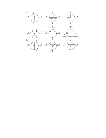
Figure 4: Typical Feynman diagrams for the contribution of scalar quarks and gluinos to the $W/Z$–boson self–energies at the two–loop level.

The two–loop contribution of a complete quark/squark generation to the vacuum polarization functions of the electroweak gauge bosons at zero momentum–transfer have been calculated $\!{}^{{\bf?},{\bf?}}$ taking into account general mixing between scalar quarks and allowing for all particles to have different masses. The results were derived by two independent calculations using different methods: one by evaluating the unrenormalised self-energies and the mass and self-energy counterterms almost by hand and the other by using the package FeynArts $\!{}^{{\bf?}}$ where the relevant part of the MSSM has been implemented. The two independent calculations allowed for thorough checks of the final results.

The two–loop Feynman diagrams of Fig. 4 have to be supplemented by the corresponding counterterm insertions into the one–loop diagrams. By virtue of the Ward identity, the vertex and wave–function renormalisation constants cancel each other. The mass renormalisation has been performed in the on–shell scheme, where the mass is defined as the pole of the propagator. The mixing angle renormalisation is performed in such a way that all transitions from $\tilde{q}_{i}\leftrightarrow\tilde{q}_{j}$ which do not depend on the loop–momenta in the two–loop diagrams are canceled; this renormalisation condition is equivalent to the one used in Ref. $\!{}^{{\bf?}}$ for scalar quark decays. With this choice of the mass and mixing angle renormalisation, the pure scalar quark diagrams in Fig. 4a that contribute to the transverse parts of the gauge–boson self–energies are canceled.

In order to discuss the results, one can first concentrate on the contribution of the gluonic corrections, Fig. 4a, and the corresponding counterterms, which has a very simple analytical expression. Indeed, the contribution of the $(\tilde{t},\tilde{b})$ doublet to the $\rho$ parameter, including the two–loop gluon exchange and pure scalar quark diagrams is very simple if the mixing in the $\tilde{b}$ sector is neglected; it is given by:

$$\Delta\rho^{\rm SUSY}_{1}=\frac{G_{F}\alpha_{s}}{4\sqrt{2}\pi^{3}}\left[-s_{t}^{2}c_{t}^{2}F_{1}\left(m_{\tilde{t}_{1}}^{2},m_{\tilde{t}_{2}}^{2}\right)+c_{t}^{2}F_{1}\left(m_{\tilde{t}_{1}}^{2},m_{\tilde{b}_{L}}^{2}\right)+s_{t}^{2}F_{1}\left(m_{\tilde{t}_{2}}^{2},m_{\tilde{b}_{L}}^{2}\right)\right]$$ (10)

where the two–loop function $F_{1}(x,y)$ is given in terms of dilogarithms by

$$F_{1}(x,y)=a_{+}-2\frac{xy}{a_{-}}\log\frac{x}{y}\left[2+\frac{x}{y}\log\frac{x}{y}\right]+\frac{a_{+}x^{2}}{a_{-}^{2}}\log^{2}\frac{x}{y}-2a_{-}{\rm Li}_{2}\left(1-\frac{x}{y}\right)$$ (11)

with $a_{\pm}=x\pm y$. This function is symmetric in the interchange of $x$ and $y$. As in the case of the one–loop function $F_{0}$, it vanishes for degenerate masses, $F_{1}(x,x)=0$, while in the case of large mass splitting it increases with the heavy scalar quark mass squared: $F_{1}(x,0)=x(1+\pi^{2}/3)$.

The two–loop gluonic SUSY contribution to $\Delta\rho$ is shown in Fig. 5 as a function of the common scalar mass $m_{\tilde{q}}$, for the two scenarios discussed previously: $\theta_{\tilde{t}}=0$ and $\theta_{\tilde{t}}\simeq-\pi/4$. As can be seen, the two–loop contribution is of the order of 10 to 15% of the one–loop result. Contrary to the SM case [and to many QCD corrections to electroweak processes in the SM, see Ref. $\!{}^{{\bf?}}$ for a review] where the two–loop correction screens the one–loop contribution, $\Delta\rho_{1}^{\rm SUSY}$ has the same sign as $\Delta\rho_{0}^{\rm SUSY}$. For instance, in the case of degenerate $\tilde{t}$ quarks with masses $m_{\tilde{t}}\gg m_{\tilde{b}}$, the result is the same as the QCD correction to the $(t,b)$ contribution in the SM, but with opposite sign. The gluonic correction to the contribution of scalar quarks to the $\rho$ parameter will therefore enhance the sensitivity in the search of the virtual effects of scalar quarks in high–precision electroweak measurements.

Figure 5: Gluon exchange contribution to the $\rho$ parameter at two–loop as a function of $m_{\tilde{q}}$.

The analytical expressions of the contribution of the two–loop diagrams with gluino exchange, Fig. 4b, to the electroweak gauge boson self–energies are very complicated even at zero momentum–transfer. Besides the fact that the scalar quark mixing leads to a large number of contributing diagrams, this is mainly due to the presence of up to five particles with different masses in the loops. The lengthy expressions are given in Ref. $\!{}^{{\bf?}}$. It turned out that in general the gluino exchange diagrams give smaller contributions compared to gluon exchange. Only for gluino and squark masses close to the experimental bounds they compete with the gluon exchange contributions. In this case, the gluon and gluino contributions add up to $\sim 30\%$ of the one–loop value for maximal mixing; Fig. 6. For larger values of $m_{\tilde{g}}$, the contribution decreases rapidly since the gluinos decouple for high masses.

Finally, let us note that for the diagrams in Fig. 4a analytical expressions for arbitrary momentum–transfer can be obtained as discussed in Ref. $\!{}^{{\bf?}}$. With the present computational knowledge of two–loop radiative corrections, analytical exact results for the diagrams involving gluino exchange, Fig. 4b, cannot be obtained for arbitrary $q^{2}$; either approximations like heavy mass expansions or numerical methods have to be applied.

Figure 6: Contribution of the gluino exchange diagrams to $\Delta\rho_{1}^{\rm SUSY}$ for two values of $m_{\tilde{g}}$.

5 Summary

I have discussed the possibility of detecting the virtual effects of the new particles predicted by supersymmetric extensions of the Standard Model in the high–precision electroweak observables measured at LEP/SLC, the Tevatron and CLEO. In view of the experimental accuracies on these observables and the experimental limits on the SUSY particle masses, the two only observables where these new effects might show up are the $\rho$ parameter and the radiative decay $b\to s\gamma$. The experimental values of the two quantities agree well, for the time being, with Standard Model expectations and rather strong constraints on the MSSM parameter space can be obtained. In the not too far future, more experimental accuracy can be achieved giving the hope that some deviations from SM predictions might appear, thus showing for the first time an indirect manifestation of SUSY.

In order to make an accurate comparison between experimental and theoretical values, high order effects must be included in the prediction for these two observables. The next–to–leading order SUSY–QCD corrections have been made available for both of them. In the last part of this lecture, I tried to summarize the way, the techniques, and the complications of performing such calculations, taking as an example the two–loop SUSY–QCD corrections to the $\rho$ parameter.

References

References

- [1] For reviews on SUSY see: H.P. Nilles, Phys. Rep. 110 (1984) 1; H.E. Haber and G.L. Kane, Phys. Rep. 117 (1985) 75; M. Drees and S. Martin, hep-9504324; S. Martin, hep-ph9709356; J. Bagger, hep-ph/9604232.
- [2] Peter Zerwas, Lectures given at this school.
- [3] For a review on the Higgs sector of the MSSM, see J.F. Gunion, H.E. Haber, G.L. Kane and S. Dawson, “The Higgs Hunter’s Guide”, Addison–Wesley, Reading 1990.
- [4] A summary of the experimental data available in January 1999 is given e.g. in: A. Djouadi, S. Rosier-Lees et al., hep-ph/9901246.
- [5] See the Lectures given by Luc Pape, these proceedings.
- [6] M. Carena et al, in “Higgs Physics at LEP2”, hep-ph/9602250; G.F. Giudice et al., in “Searches for New Physics at LEP2”, hep-ph/9602207.
- [7] Workshop “Physics at RunII – Higgs/Supersymmetry”, 1998, Fermilab, M. Carena and H. Haber (eds.), to appear.
- [8] ATLAS Collaboration, Technical Proposal, Report CERN–LHCC 94–43; CMS Collaboration, Technical Proposal, Report CERN–LHCC 94–38.
- [9] See e.g.: E. Accomando et al., Phys. Rep. 299 (1998) 1; P.M. Zerwas et al., ECFA–DESY Workshop, hep-ph/9605437; NLC and NLC ZDR Design and Physics Working Groups, hep-ex/9605011; A. Djouadi, hep-ph/9910449.
- [10] For a summary of data on EW observables available in Januray 1999, see the talk of D. Karlen at ICHEP98, Vancouver.
- [11] For a theoretical overview of the EW data, see W. Hollik, hep-ph/9811313, talk at the ICHEP98, Vancouver.
- [12] See the review talk by R. Partridge at the ICHEP98, Vancouver.
- [13] C. S. Lim, T. Inami and N. Sakai, Phys. Rev. D29 (1984) 1488; E. Eliasson, Phys. Lett. B147 (1984) 65. ; Z. Hioki, Prog. Theo. Phys. 73 (1985) 1283; J. A. Grifols and J. Sola, Nucl. Phys. B253 (1985) 47; B. Lynn, M. Peskin and R. Stuart, CERN Report 86–02, p. 90; R. Barbieri, M. Frigeni, F. Giuliani and H.E. Haber, Nucl. Phys. B341 (1990) 309; A. Bilal, J. Ellis and G. Fogli, Phys. Lett. B246 (1990) 459; M. Drees, K. Hagiwara and A. Yamada, Phys. Rev. D45, (1992) 1725; P. Chankowski et al., Nucl. Phys. B417, 101 (1994); D. Garcia and J. Solà, Mod. Phys. Lett. A9 (1994) 211.
- [14] M. Drees and K. Hagiwara, Phys. Rev. D42, 1709 (1990).
- [15] M. Veltman, Nucl. Phys. B123, 89 (1977).
- [16] A. Djouadi and C. Verzegnassi, Phys. Lett. B195 265 (1987).
- [17] A. Djouadi, Nuovo Cim. A100, 357 (1988); B.A. Kniehl, J.H. Kuhn and R.G. Stuart, Phys. Lett. B214 (1988) 621; B.A. Kniehl, Nucl. Phys B347 (1990) 86; A. Djouadi and P. Gambino, Phys. Rev. D49 (1994) 3499 and Phys. Rev. D49 (1994) 4705. The three–loop result for is also available: K. Chetyrkin, J. Kühn and M. Steinhauser, Phys. Rev. Lett. 75, 3394 (1995); L. Avdeev J. Fleischer, S.M. Mikhailov and O. Tarasov, Phys. Lett. B336, 560 (1994).
- [18] W. Hollik, Z. Phys. C32 (1986) 291 and Z. Phys. C37 (1988) 569; S. Bertolini, Nucl. Phys. B272 (1986) 77.
- [19] A. Djouadi, M. Drees and H. König, Phys. Rev. D48 (1993) 3081; K. Hagiwara and H. Murayama, Phys. Lett. B246 (1990) 533.
- [20] A. Denner et al., Z. Phys. C51 (1991) 695; A. Djouadi, J.L. Kneur and G. Moultaka, Phys. Lett. B242 (1990) 265.
- [21] A. Djouadi, G. Girardi, W. Hollik, F. Renard, C. Verzegnassi, Nucl. Phys. B349 (1991) 48; M. Boulware and D. Finnell, Phys. Rev. D44 (1991) 2054.
- [22] See e.g. W. de Boer et al., hep-ph/9609209; J. Wells, C. Kolda and G.L. Kane, Phys. Lett. 338 (1994) 219; D. Garcia, R. Jiménez and J. Solà, Phys. Lett. B347 (1995) 309; B347 (1995) 321; D. Garcia and J. Solà, Phys. Lett. B357 (1995) 349; P. Chankowski and S. Pokorski, Nucl. Phys. B475 (1996) 3.
- [23] S. Bertolini et al., Nucl. Phys. B353, 591 (1991); R. Barbieri and G. Giudice, Phys. Lett. B309, 86 (1993); F. Borzumati, M. Olechowski and S. Pokorski, Phys. Lett. B349 (1995) 311.
- [24] For recent global fits of the MSSM, see: J. Erler and D. M. Pierce, Nucl. Phys. B526 (1998) 53-80; W. de Boer, H.J. Grimm, A.V. Gladyshev and D.I. Kazakov, Phys. Lett. B438 (1998) 281.
- [25] G.C. Cho, K. Hagiwara, C. Kao, R. Szalapski, hep-ph/9901351.
- [26] M. Ciuchini, G. Degrassi, P. Gambino and G.F. Giudice, Nucl. Phys. B534 (1998) 3; F. Borzumati and Ch. Phys. Rev. D58 (1998) 074004; F. Borzumati, Ch. Greub, T. Hurth and D. Wyler, hep-ph/9911245.
- [27] A. Djouadi, P. Gambino, S. Heinemeyer, W. Hollik, C. Jünger and G. Weiglein, Phys. Rev. Lett. 78 (1997) 3626.
- [28] A. Djouadi, P. Gambino, S. Heinemeyer, W. Hollik, C. Jünger and G. Weiglein, Phys. Rev. D57 (1998) 4179.
- [29] G. ’t Hooft and M. Veltman, Nucl. Phys. B44 (1972) 189; P. Breitenlohner and D. Maison, Commun. Math. Phys. 52 (1977) 11.
- [30] S. Martin and M. Vaughn, Phys. Lett. B318 (1993) 331; I. Jack, D.R.T. Jones and K.L. Roberts, Z. Phys. C63 (1994) 151.
- [31] W. Siegel, Phys. Lett. B84 (1979) 193; D. M. Capper, D.R.T. Jones, P. van Nieuwenhuizen, Nucl. Phys. B167 (1980) 479.
- [32] A. Djouadi, M. Spira, P.M. Zerwas, Phys. Lett. B264 (1991) 440 and Phys. Lett. B311 (1993) 255; M. Spira et al., Nucl. Phys. B453 (1995) 17.
- [33] J. Küblbeck, M. Böhm, A. Denner, Comput. Phys. Commun 60, 165 (1990).
- [34] H. Eberl et al., Nucl.Phys. B472 (1996) 481; A. Djouadi, W. Hollik and C. Junger, Phys. Rev. D55 (1997) 6975; A. Arhrib et al., Phys. Rev. D57 (1998) 5860; S. Kraml, H. Eberl, A. Bartl, W. Majerotto and W. Porod, Phys. Lett. B386 (1996) 175; W. Beenakker, R. Hopker, T. Plehn and P.M. Zerwas, Z. Phys. C75 (1997) 349.
- [35] B. Kniehl, Int. J. Mod. Phys. A10 (1995) 443.