HD-THEP-99-49
ITFA-99-33
November 1999

Divergences in Real-Time Classical Field Theories at Non-Zero Temperature

Abstract

The classical approximation provides a non-perturbative approach to time-dependent problems in finite temperature field theory. We study the divergences in hot classical field theory perturbatively. At one-loop, we show that the linear divergences are completely determined by the classical equivalent of the hard thermal loops in hot quantum field theories, and that logarithmic divergences are absent. To deal with higher-loop diagrams, we present a general argument that the superficial degree of divergence of classical vertex functions decreases by one with each additional loop: one-loop contributions are superficially linearly divergent, two-loop contributions are superficially logarithmically divergent, and three- and higher-loop contributions are superficially finite. We verify this for two-loop SU($N$) self-energy diagrams in Feynman and Coulomb gauges. We argue that hot, classical scalar field theory may be completely renormalized by local (mass) counterterms, and discuss renormalization of SU($N$) gauge theories.

1 Introduction

The classical approximation [1] is a useful tool for the study of infrared properties of quantum fields at high temperature [2, 3, 4, 5, 6, 7, 8, 9], which may be applied to calculate non-perturbative phenomena such as the Chern-Simons diffusion rate [10, 11, 12] (relevant for theories of baryogenesis [13]) and the dynamics of the electroweak phase transition [14], as well as real-time (plasmon) properties of hot non-abelian gauge theories [15]. The classical theory is expected to be a good approximation at low-energy because the classical limit $\hbar\rightarrow 0$ and the low-energy limit of the Bose-Einstein distribution function $n$ yield the same result:

$$n(\omega_{{\mathbf{k}}})=\frac{1}{\exp(\beta\hbar\omega_{{\mathbf{k}}})-1}\rightarrow\frac{1}{\beta\hbar\omega_{{\mathbf{k}}}}\equiv n_{\rm cl}(\omega_{{\mathbf{k}}}),\quad\hbar\omega_{{\mathbf{k}}}\ll T,$$ (1.1)

where $\omega_{{\mathbf{k}}}=\sqrt{{\mathbf{k}}^{2}}$ is the frequency at wave-number ${\mathbf{k}}$ and $\beta=1/T$ the inverse temperature. Classical correlation functions are determined by a set of field equations in Minkowski space and a thermal average over the initial fields at some (arbitrary) initial time. In perturbation theory, classical vertex functions can be obtained by taking the limit $\hbar\rightarrow 0$ of the quantum expressions, which amounts to the replacement (1.1) of the Bose-Einstein distribution function by the classical distribution function. The resulting $\hbar$’s in the denominator are compensated by a positive power of $\hbar$’s arising from the loop counting of the diagrams under consideration, such that in the classical limit a non-trivial expression (and loops) remain.

The replacement (1.1) is a good approximation for infrared-dominated diagrams, but it changes the ultraviolet behavior of the theory and introduces classical (Rayleigh-Jeans-type) divergences. When the classical theory is considered as a low-energy effective theory, these divergences can be regularized by introducing a cut-off of the order of the temperature, $\Lambda\sim T/\hbar$. Since in a weakly coupled theory the temperature is large compared to dynamically generated energy scales such as $g^{2}T$, the resulting cut-off dependences are a direct reflection of the divergences of the classical theory. The general strategy to improve the effective theory is to include counterterms that reduce the cut-off dependence. In particular, if a complete set of counterterms can be specified, the cut-off may be sent to infinity and the theory is renormalized. It is clear that a knowledge of the divergences is necessary to determine the appropriate counterterms. We will assume that these divergences will be tractable in perturbation theory.

In the case of a $\lambda\phi^{4}$ scalar field theory the divergences have been studied in classical perturbation theory for the two-point function up to two loops and the four-point function up to one-loop [6, 7, 8]. It was found that the one-loop resp. two-loop correction to the self-energy is linearly resp. logarithmically divergent, and that the one-loop correction to the four-point function is finite [7]. In $3+1$ dimensional gauge theories on the other hand, the attention has mainly been restricted to the classical equivalent of the quantum hard thermal loop (HTL) expressions [16, 17, 18], which introduce linear divergences in the classical theory [3, 4, 5]. Numerical studies using a HTL improved effective theory [3, 19, 20] can be found in [21, 22, 23]. An analysis of the divergences in the classical theory that goes beyond the HTL limit at one-loop, or to higher loops, has not yet been performed for gauge theories. Our aim in this paper is therefore to give a more complete analysis of the divergence structure of hot, real-time classical field theory.

A different kind of effectively classical theory beyond the HTL regime was constructed in [24], by integrating out the scales $T$ and $gT$ in a leading log approximation. It takes the form of a Langevin equation and is free from ultraviolet divergences [25]. For a numerical implementation, see [26]. However, our focus in this paper is on classical Yang-Mills theory as it stands, without any further integrating out to construct an effective theory.

We shall argue that both in SU($N$) gauge theory and in scalar field theory with $\phi^{3}$ and $\phi^{4}$ interaction terms the divergences are restricted to one- and two-loop (sub)diagrams. It will be shown that classical one-loop diagrams that correspond to HTL’s in the quantum theory lead to linear divergences, while other one-loop diagrams are finite in the classical theory. Also we present a general argument that two-loop diagrams can at most give logarithmic divergences. This is explicitly verified for two-loop self-energy corrections in SU($N$) and scalar theories.

The paper is organized as follows. Classical one-loop diagrams are analyzed in the next section, and diagrams with two loops and more in section 3. In section 4 the possibility of absorbing the divergences with counterterms is discussed. The final section contains the conclusions. Throughout the paper expressions for classical diagrams are obtained by taking the $\hbar\to 0$ limit in the quantum expressions. The validity of this is discussed in more detail in appendix A, where a set of classical Feynman rules is presented for hot scalar fields.

2 One-loop

2.1 Linear divergences: classical HTL’s

The one-loop linear divergences of the classical theory are closely related to the (quantum) hard thermal loops discovered by Braaten and Pisarski [16] (see also [17, 28, 29]). For instance, the divergent part of the classical self-energy in SU($N$) gauge theory can be obtained as the classical limit of the HTL self-energy [3, 4]. To be specific, the spatial part of the retarded HTL self-energy reads

$$\Pi_{HTL,ij}^{ab}(P)=-2\delta^{ab}g^{2}\hbar N\int\frac{d^{3}k}{(2\pi)^{3}}\,\hat{k}_{i}\hat{k}_{j}n^{\prime}(\omega_{{\mathbf{k}}})\frac{p^{0}}{p^{0}-{\bf\hat{k}}\cdot{\mathbf{p}}},$$ (2.1)

where here and in the following the external frequency $p^{0}$ is taken real with a small imaginary part to obtain the retarded self-energy, i.e. $p^{0}\equiv\mbox{Re}(p^{0})+i\epsilon$, and

$$n^{\prime}(\omega_{{\mathbf{k}}})=\frac{dn(\omega_{{\mathbf{k}}})}{d\omega_{{\mathbf{k}}}}.$$ (2.2)

As usual in the HTL approximation, the radial and angular integration decouple and the radial integration determines the plasmon frequency

$$\omega_{\rm pl}^{2}=-\frac{1}{3\pi^{2}}g^{2}\hbar N\int_{0}^{\infty}dk\,k^{2}n^{\prime}(k)=\frac{1}{9}g^{2}N\frac{T^{2}}{\hbar}.$$ (2.3)

The classical self-energy corresponding to (2.1) is obtained by taking the $\hbar\rightarrow 0$ limit, before the integration over ${\mathbf{k}}$ is performed. This simply amounts to replacing the Bose-Einstein distribution function by the classical distribution function, as in (1.1). The classical self-energy is non-vanishing, since the $\hbar$ in the prefactor of (2.1) is compensated by the $\hbar$ in the denominator of the classical distribution function. The resulting radial integral is linearly divergent and to handle this we introduce a cut-off in the classical distribution function $n_{\rm cl}(\omega_{{\mathbf{k}}})\rightarrow n_{\rm cl}(\omega_{{\mathbf{k}}})\theta(\Lambda-k)$. This particular way of introducing a momentum cut-off in loop integrals does not lead to problems with gauge invariance, which can be most easily understood from the gauge propagator of Landshoff and Rebhan [30] and is explained in appendix A.2. The result is a linearly divergent classical plasmon frequency

$$\omega_{\rm pl,cl}^{2}=\frac{2}{3\pi^{2}}g^{2}NT\Lambda.$$ (2.4)

The relation between the quantum plasmon frequency (2.3) and the classical analogue (2.4) is that the Bose-Einstein distribution function effectively introduces a cut-off of the order of the temperature on the integration, $\Lambda\sim T/\hbar$. Since the angular integration is completely decoupled, the dependence on the external momenta of the linearly divergent contribution to the classical self-energy and HTL self-energy are equal. All of this is well-known [3, 4].

Hard thermal loops are the leading contributions to vertex functions for soft external momenta $|p^{0}|,p\sim gT$. Power counting reveals that one-loop diagrams, with any number of external gauge fields, contain a HTL contribution. The fact that the external momenta are small compared to the internal momentum $k\sim T$ allows for several simplifications in the calculation of HTL’s. As a result all HTL’s are proportional to the plasmon frequency squared (2.3) [16, 18].

Divergences in classical field theories have a similar behavior, since here also the internal momenta $k\sim\Lambda$ are much larger than the external momenta. In fact, all classical HTL’s have the proportionality factor (2.4). Therefore, all classical HTL’s are linearly divergent.

Other one-loop contributions in the quantum theory are smaller by a factor $p/k\sim p/T$. In the classical limit these subleading contributions give a factor $p/k\sim p/\Lambda$, which reduces the degree of divergence. Therefore we may conclude that all linear divergences at one-loop are given by the classical HTL’s.

2.2 No logarithmic divergences

Next we will argue that there are no logarithmic divergences at one-loop in the classical theory. Firstly, we discuss one particular example in SU($N$) gauge theory explicitly, which is the spatial part of the self-energy in the Feynman gauge. A convenient starting point is the expression in the quantum theory, which reads

$$\Pi_{ij}^{ab}(P) = \delta^{ab}g^{2}\hbar N\int\frac{d^{3}k}{(2\pi)^{3}}\Bigg{\{}g_{ij}\frac{2n(\omega_{{\mathbf{k}}})+1}{\omega_{{\mathbf{k}}}}-\frac{A_{ij}}{4\omega_{{\mathbf{k}}}\omega_{{\mathbf{p}}+{\mathbf{k}}}}\times$$

$$\bigg{(}[n(\omega_{{\mathbf{k}}})+n(\omega_{{\mathbf{p}}+{\mathbf{k}}})+1]\Big{[}\frac{1}{p^{0}+\omega_{{\mathbf{k}}}+\omega_{{\mathbf{p}}+{\mathbf{k}}}}-\frac{1}{p^{0}-\omega_{{\mathbf{k}}}-\omega_{{\mathbf{p}}+{\mathbf{k}}}}\Big{]}$$

$$+[n(\omega_{{\mathbf{k}}})-n(\omega_{{\mathbf{p}}+{\mathbf{k}}})]\Big{[}\frac{1}{p^{0}-\omega_{{\mathbf{k}}}+\omega_{{\mathbf{p}}+{\mathbf{k}}}}-\frac{1}{p^{0}+\omega_{{\mathbf{k}}}-\omega_{{\mathbf{p}}+{\mathbf{k}}}}\Big{]}\bigg{)}\Bigg{\}},$$

with

$$A_{ij}=\frac{1}{2}\left[8k_{i}k_{j}+5p_{i}k_{j}+3k_{i}p_{j}+4(p^{2}-p_{0}^{2})g_{ij}-2p_{i}p_{j}\right].$$ (2.6)

This diagram contains of course the HTL self-energy (2.1). As before, the classical expression is obtained by taking $\hbar$ to zero. The non-thermal contribution from the “1” in the first and second line vanishes as $\hbar$ goes to zero.

From the previous section we know that contributions to the self-energy (LABEL:onels-e) are at most linearly divergent. The classical limit of the momentum-independent tadpole-like contribution in the first line is indeed linearly divergent. For the contribution proportional to $A_{ij}$, it implies that the contributions bilinear in the external momenta, i.e. the terms proportional to $p_{i}p_{j}$ or $p^{2}\delta_{ij}$, can only give ultraviolet finite contributions, and that the terms linear in the external momenta (terms proportional to $k_{i}p_{j}$ or $p_{i}k_{j}$) may give logarithmic divergences. The contributions proportional to $k_{i}k_{j}$ may contain logarithmic divergences besides the linearly divergent contributions as well.

To obtain the linearly and logarithmically divergent contributions we expand the integrand in $1/k$, so that we can estimate the ultraviolet behavior of the integrand by power counting. The contribution from the second line reads

$$\frac{A_{ij}}{4\omega_{{\mathbf{k}}}\omega_{{\mathbf{p}}+{\mathbf{k}}}}[n_{\rm cl}(\omega_{{\mathbf{k}}})+n_{\rm cl}(\omega_{{\mathbf{p}}+{\mathbf{k}}})]\Big{[}\frac{1}{p^{0}+\omega_{{\mathbf{k}}}+\omega_{{\mathbf{p}}+{\mathbf{k}}}}-\frac{1}{p^{0}-\omega_{{\mathbf{k}}}-\omega_{{\mathbf{p}}+{\mathbf{k}}}}\Big{]}$$

$$=\frac{A_{ij}}{4k^{2}}\left\{\frac{2}{k}n_{\rm cl}(k)+({\mathbf{p}}\cdot{\bf\hat{k}})\Big{[}\frac{1}{k}n^{\prime}_{\rm cl}(k)-\frac{3}{k^{2}}n_{\rm cl}(k)\Big{]}+{\cal O}(k^{-4})\right\}.$$ (2.7)

The first term on the second line, with $A_{ij}\propto k_{i}k_{j}$, is part of the HTL contribution. The second term between curly brackets, and the first term with $A_{ij}\propto p_{i}k_{j},k_{i}p_{j}$, contain the contributions proportional to $k^{-3}$, and these may give a logarithmic divergence after integration. However, it turns out that these contributions are odd under the transformation ${\bf\hat{k}}\rightarrow-{\bf\hat{k}}$ and therefore they vanish upon integration. The other terms, including those indicated with ${\cal O}(k^{-4})$, are ultraviolet finite by power counting.

Similarly, the third line can be expanded, and after some algebra it can be written as

$$\frac{A_{ij}}{4\omega_{{\mathbf{k}}}\omega_{{\mathbf{p}}+{\mathbf{k}}}}[n(\omega_{{\mathbf{k}}})-n(\omega_{{\mathbf{p}}+{\mathbf{k}}})]\Big{[}\frac{1}{p^{0}-\omega_{{\mathbf{k}}}+\omega_{{\mathbf{p}}+{\mathbf{k}}}}-\frac{1}{p^{0}+\omega_{{\mathbf{k}}}-\omega_{{\mathbf{p}}+{\mathbf{k}}}}\Big{]}$$

$$=\frac{A_{ij}}{4k^{2}}\frac{2{\mathbf{p}}\cdot{\bf\hat{k}}}{p_{0}^{2}-({\mathbf{p}}\cdot{\bf\hat{k}})^{2}}\Bigg{\{}({\mathbf{p}}\cdot{\bf\hat{k}})n^{\prime}_{\rm cl}(k)+\frac{1}{2}({\mathbf{p}}\cdot{\bf\hat{k}})^{2}n^{\prime\prime}_{\rm cl}(k)$$

$$-\frac{1}{k}n^{\prime}_{\rm cl}(k)\bigg{[}({\mathbf{p}}\cdot{\bf\hat{k}})^{2}-p_{0}^{2}\frac{p^{2}-({\mathbf{p}}\cdot{\bf\hat{k}})^{2}}{p_{0}^{2}-({\mathbf{p}}\cdot{\bf\hat{k}})^{2}}\bigg{]}+{\cal O}(k^{-4})\Bigg{\}}.$$ (2.8)

The first term on the second line, again with $A_{ij}\propto k_{i}k_{j}$, is part of the HTL contribution, and is proportional to $k^{-2}$. The other terms contain a contribution proportional to $k^{-3}$, which after integration could yield a logarithmic divergence. However, just as in the previous case these contributions are odd under the transformation ${\bf\hat{k}}\rightarrow-{\bf\hat{k}}$ and they vanish upon integration. The remaining terms are ultraviolet finite.

Therefore, we conclude that there is no logarithmic divergence in the spatial part of the retarded classical self-energy in the Feynman gauge. In a similar manner, we have also verified that the spatial part of the three-point vertex contains no logarithmic divergences.

The reason for the vanishing of possible logarithmically divergent contributions lies in the behavior of the self-energy and the vertex functions under parity (P) and time reversal (T). The spatial part of the self-energy discussed here is invariant under ${\mathbf{p}}\to-{\mathbf{p}}$, and $p^{0}\to-p^{0}$ in combination with complex conjugation (i.e. $p^{0}+i\epsilon\to-(p^{0}+i\epsilon)$ in (LABEL:onels-e)). The point is that the expansion in $1/k$ turns out to be an expansion in PT odd (dimensionless) functions of $p^{0}$ and ${\mathbf{p}}$. Since the linearly divergent HTL contributions to the self-energy are even under P and T, the logarithmically divergent contributions are odd and should therefore vanish. This argument extends to the temporal part of the self-energy as well as to other vertex functions.

Finally we would like to remark that the vanishing of logarithmic divergences holds in general Coulomb or covariant gauges, since the corresponding gauge fixing term does not break PT invariance, and the same argument can be applied.

2.3 Classical self-energy: explicit result

The analysis presented above is useful for a general understanding. However, in some cases it is possible to actually calculate the loop integrals and avoid an expansion in $1/k$. Here we give one of those explicit results in SU($N$) theory.

We calculate the diagonal ($ii$) part of the classical one-loop retarded self-energy in the Feynman gauge in appendix B, and the result reads

$$\Pi_{ii,\rm cl}^{ab}(P)=\delta^{ab}g^{2}N\left[\frac{T\Lambda}{\pi^{2}}\frac{p^{0}}{p}\ln\frac{p^{0}+p}{p^{0}-p}+\frac{T}{4\pi}\bigg{(}ip^{0}-\frac{3p^{2}-4p_{0}^{2}}{2p}i\ln\frac{p^{0}+p}{p^{0}-p}\bigg{)}\right].$$ (2.9)

The real and imaginary parts can be obtained in the usual way, using

$$\ln\frac{p^{0}+p}{p^{0}-p}=\ln\left|\frac{p^{0}+p}{p^{0}-p}\right|-i\pi\theta(p^{2}-p_{0}^{2}).$$ (2.10)

The linear divergence is precisely the equivalent of the hard thermal loop contribution, which follows from the replacement $T\Lambda/\pi^{2}\to T^{2}/(6\hbar)$. The finite terms are exactly equal to the terms linear in $T$ that are obtained in a high temperature expansion in the quantum theory, as can be checked explicitly [29, 32]. There are no other terms. The $p^{0}\to 0$ limit equals the well-known result from the quantum theory in the Feynman gauge [33]

$$\Pi_{ii,\rm cl}^{ab}(0,{\mathbf{p}})=-\delta^{ab}g^{2}N\frac{3pT}{8}.$$ (2.11)

Note that in this limit the leading-order (gauge-dependent) behavior is completely determined by classical physics.

To conclude the one-loop analysis, the above described situation can be understood also directly by keeping $\hbar$ in the high-temperature expression of the quantum theory. The high-temperature expansion then has the form [29, 32]

$$\Pi_{ii\rm}^{ab}(P)=\delta^{ab}g^{2}N\Bigg{[}\frac{T^{2}}{\hbar}\Pi_{-1}(P)+T\Pi_{0}(P)+\left(\hbar\ln\frac{T}{\hbar\mu}\right)\Pi_{\rm log}(P)+\hbar\Pi_{1}(P)+{\cal O}(\frac{\hbar^{3}}{T^{2}})\Bigg{]},$$ (2.12)

where $\mu$ is the renormalization scale. The term proportional to $T^{2}$ is the HTL part, which turns into the linearly divergent term when $\hbar\to 0$, and the second term in this expansion is the finite term in the classical theory. All the other terms vanish when $\hbar\to 0$.

3 Two-loop and beyond

3.1 Degree of divergence

In this section we study the degree of divergence of higher-loop diagrams in the classical theory. In the first part we shall argue that the superficial degree of divergence of the self-energy decreases by one with each loop, starting with the one-loop linear divergence. Then we will check this statement explicitly for a number of diagrams. We shall argue that the same is true for classical vertex functions in section 3.3.

To make the argument for the self-energy, we start with the following basic assumption: in the high-temperature limit the retarded self-energy in the quantum theory scales according to its dimension, i.e., the quantum retarded gluon self-energy behaves as

$$\Pi_{\mu\nu}(P)=T^{2}\bar{\Pi}_{\mu\nu}(p^{0}/p,{\bf\hat{p}},g)+T^{2}{\cal O}(P/T),$$ (3.1)

for high temperatures, fixed external momentum and frequency, and a renormalization scale of the order of the temperature $\mu\sim T$. This assumption consists of two parts: The contribution of diagrams with hard momenta $K\sim T$ on all internal lines gives a $T^{2}$ contribution to the self-energy. Contributions that are excluded in (3.1) are of the form $g^{2L}T^{2}(T/P)^{m}$ for $m>0$ and with $L$ indicating the number of loops. For fixed external momenta and high temperatures such terms become larger than the one-loop (HTL) contribution $g^{2}T^{2}$, so they invalidate a loop expansion. Therefore the assumed absence of these contributions can be re-expressed by saying that we assume that hard modes are perturbative. The other part of the assumption is that also diagrams with soft internal momenta give a $T^{2}$ contribution. This relies on the belief that infrared divergences are controlled by induced masses, which are proportional to the temperature, such as the electric and magnetic masses in SU($N$) gauge theories.

Let us then consider a classical contribution to the self-energy containing $M$ distribution functions. To be able to compare the degree of divergence of such a contribution with the quantum expression, we regard the temperature in the quantum self-energy as a particular ultraviolet cut-off, and using the assumption (3.1) we count the degree of divergence as 2. Since every classical distribution function gives rise to an extra energy in the denominator when compared to the quantum diagram, the classical contribution to the self-energy with $M$ distribution functions has then a superficial degree of divergence $2-M$.

To complete the argument, we now use that the number of distribution functions $M$ can be related to the number of loops $L$ in the following manner [34, 35]. One way to obtain the retarded self-energy is by using the imaginary-time or Matsubara formalism [36, 18]. One first performs the sums over the discrete loop frequencies and then analytically continues the external frequencies to real values with a small positive part to incorporate the appropriate retarded boundary conditions. In the imaginary-time formalism the number of loops equals the number of Matsubara frequency summations. Using the method of contour integration to perform these sums, each sum gives rise to one ‘coth’ function, either with positive or negative energy. Explicitly, each sum gives a factor [34, 35]

$$\frac{1}{2}\coth\frac{s\hbar\omega}{2T}=n(s\omega)+\frac{1}{2}=s[n(\omega)+\frac{1}{2}],\;\;\;\;s=\pm.$$ (3.2)

Hence, the resulting expressions are of the form of spatial momentum integrals over Bose-Einstein distribution functions, where the number of distribution functions is equal to or less than the numbers of loops. The classical limit can now be taken by replacing $n(\omega)+\frac{1}{2}\to T/(\hbar\omega)$, such that the $\hbar$’s counting the loops cancel against the $1/\hbar$’s from the distribution functions. After taking the classical limit, only the leading term, which has as many distribution functions as loops, remains and the number of classical distribution functions $M$ in a given diagram is counted by the number of loops, $M=L$. Note that this applies not only to the self-energy diagrams but to vertex functions as well. It follows then that the superficial degree of divergence of a classical diagram is given by $2-L$, such that the classical one-loop contribution to the self-energy is superficially linearly divergent, the two-loop contribution is superficially logarithmically divergent, and higher-loop contributions are superficially finite.

3.2 Two-loop self-energy diagrams

We now want to verify the general argument of the previous section for the two-loop self-energy diagrams appearing in SU($N$) and scalar field theory. We do not discuss diagrams which have a one-loop self-energy subdiagram (and hence also a linear subdivergence), but we concentrate on the two-loop diagrams as shown in fig. 1. Furthermore, since we are only interested in the structure of ultraviolet divergences, i.e. in power counting, we do not need to make a distinction between gauge field propagators in the Feynman gauge and ghost propagators in the loops.

Figure 1: Two-loop diagrams. The setting sun diagram (a) and diagram (b) are discussed in section 3.2, and diagram (c) is treated in appendix C.

Let us, as a first relatively simple example, take the two-loop setting-sun contribution (a) to the retarded self-energy as it appears in $\lambda\phi^{4}$-theory (with $\lambda=g^{2}$) and SU($N$) gauge theory. It reads

$$\Pi^{\rm(a)}(P)=\frac{1}{6}(g^{2}\hbar)^{2}\int\frac{d^{3}k}{(2\pi)^{3}}\int\frac{d^{3}k^{\prime}}{(2\pi)^{3}}\sum_{ss^{\prime}s_{1}}\frac{ss^{\prime}s_{1}}{2^{3}\omega_{{\mathbf{k}}}\omega_{{\mathbf{k}}^{\prime}}\omega_{{\mathbf{k}}_{1}}}\,\frac{1}{p^{0}+s\omega_{{\mathbf{k}}}+s^{\prime}\omega_{{\mathbf{k}}^{\prime}}+s_{1}\omega_{{\mathbf{k}}_{1}}}$$

$$\Big{\{}\left[1+n(s\omega_{{\mathbf{k}}})\right]\left[1+n(s^{\prime}\omega_{{\mathbf{k}}^{\prime}})\right]\left[1+n(s_{1}\omega_{{\mathbf{k}}_{1}})\right]-n(s\omega_{{\mathbf{k}}})n(s^{\prime}\omega_{{\mathbf{k}}^{\prime}})n(s_{1}\omega_{{\mathbf{k}}_{1}})\Big{\}},$$ (3.3)

where $\omega_{{\mathbf{k}}_{1}}=\omega_{{\mathbf{p}}-{\mathbf{k}}-{\mathbf{k}}^{\prime}}$, and the sum is over all $s$’s being $\pm$.

Note that the product of three distribution functions drops out. It is then clear that the classical limit of (3.3),

$$\Pi_{\rm cl}^{\rm(a)}(P)=\frac{1}{6}g^{4}\int\frac{d^{3}k}{(2\pi)^{3}}\int\frac{d^{3}k^{\prime}}{(2\pi)^{3}}\sum_{ss^{\prime}s_{1}}\frac{1}{2^{3}\omega_{{\mathbf{k}}}\omega_{{\mathbf{k}}^{\prime}}\omega_{{\mathbf{k}}_{1}}}\times$$

$$\hskip 28.45274pt\frac{1}{p^{0}+s\omega_{{\mathbf{k}}}+s^{\prime}\omega_{{\mathbf{k}}^{\prime}}+s_{1}\omega_{{\mathbf{k}}_{1}}}\left(s_{1}\frac{T^{2}}{\omega_{{\mathbf{k}}}\omega_{{\mathbf{k}}^{\prime}}}+s^{\prime}\frac{T^{2}}{\omega_{{\mathbf{k}}}\omega_{{\mathbf{k}}_{1}}}+s\frac{T^{2}}{\omega_{{\mathbf{k}}^{\prime}}\omega_{{\mathbf{k}}_{1}}}\right),$$ (3.4)

contains products of two classical distribution functions, in accordance with the statement that the number of loops equals the number of distribution functions. We now estimate the degree of divergence by power counting and take the loop momenta $k,k^{\prime}\sim\Lambda$. The integral measures give two contributions $\sim\Lambda^{3}$, and all single energy denominators $1/\omega$ give a factor $1/\Lambda$. The energy denominator that contains $p^{0}$ will produce, for generic large loop momenta ${\mathbf{k}},{\mathbf{k}}^{\prime}$, a hard energy denominator $\sim 1/\Lambda$. It can only produce a soft energy denominator when there is a cancellation, which is in the special case that ${\mathbf{k}}\simeq\pm{\mathbf{k}}^{\prime}$, depending on the signs of $s,s^{\prime}$ and $s_{1}$ [16]. However, for these special configurations the integral over phase space is restricted so that this will not alter the degree of divergence. We will use this estimate for energy denominators with three hard energies [16] below as well.

By power counting we therefore establish that this contribution is logarithmically divergent, as expected. This is also the result obtained in [6, 7, 8], where the classical setting sun diagram was analyzed in detail and it was shown that in fact the logarithmic divergence can be separated and is independent of the external momentum and frequency.

It should be noted that the setting sun diagram (as well as the diagrams discussed below) contains an infrared divergence for vanishing external momentum [37]. For massless $\lambda\phi^{4}$ theory, this can be cured by resumming the effective thermal mass, arising from the one-loop tadpole diagram. This has only an effect on the soft infrared modes, and does not interfere with the ultraviolet behavior of the classical diagram we investigated above.

The next example we treat is the two-loop diagram (b) in fig. 1, which appears in SU($N$) and in scalar $\phi^{3}$-theory. This particular diagram is more delicate, and it is instructive to carry out the procedure described above in detail. We will verify explicitly that in SU($N$) theory (the spatial part of) this diagram is logarithmically divergent in the Feynman gauge.

Since we are only interested in the degree of divergence of the diagram, we may ignore the color and Lorentz structure of the diagram. To indicate the momentum-dependence of the four vertices in the gauge theory, we will insert a factor $(k)^{4}_{ij}$. The precise form of the momentum insertions is unimportant for the power counting.

We have found it convenient to calculate this diagram in the imaginary-time formalism, and after performing the sums over the Matsubara frequencies, the diagram can be written as

$$\Pi^{\rm(b)}_{ij}(P)=\frac{1}{2}(g^{2}\hbar)^{2}\int\frac{d^{3}k}{(2\pi)^{3}}\int\frac{d^{3}k^{\prime}}{(2\pi)^{3}}\,(k)^{4}_{ij}\sum_{ss^{\prime}s_{1}s_{2}s_{3}}\frac{ss^{\prime}s_{1}s_{2}s_{3}}{2^{5}\omega\omega^{\prime}\omega_{1}\omega_{2}\omega_{3}}\times$$

$$\hskip 11.38092pt\frac{1}{p^{0}+s^{\prime}\omega^{\prime}+s_{3}\omega_{3}}\;\frac{1}{p^{0}+s\omega+s_{2}\omega_{2}}\;\bigg{\{}\frac{1}{-s_{3}\omega_{3}+s_{2}\omega_{2}+s_{1}\omega_{1}}\times$$

$$\hskip 28.45274pt\Big{(}[n(s_{1}\omega_{1})+1][n(s_{2}\omega_{2})+1]n(s_{3}\omega_{3})-n(s_{1}\omega_{1})n(s_{2}\omega_{2})[n(s_{3}\omega_{3})+1]\Big{)}$$

$$\hskip 11.38092pt+\frac{1}{p^{0}+s_{3}\omega_{3}+s\omega-s_{1}\omega_{1}}\times$$

$$\hskip 28.45274pt\Big{(}[n(s_{3}\omega_{3})+1][n(s\omega)+1]n(s_{1}\omega_{1})-n(s_{3}\omega_{3})n(s\omega)[n(s_{1}\omega_{1})+1]\Big{)}$$

$$\hskip 11.38092pt+\frac{1}{p^{0}+s^{\prime}\omega^{\prime}+s_{2}\omega_{2}-s_{1}\omega_{1}}\times$$

$$\hskip 28.45274pt\Big{(}[n(s^{\prime}\omega^{\prime})+1][n(s_{2}\omega_{2})+1]n(s_{1}\omega_{1})-n(s^{\prime}\omega^{\prime})n(s_{2}\omega_{2})[n(s_{1}\omega_{1})+1]\Big{)}$$

$$\hskip 11.38092pt+\frac{1}{s^{\prime}\omega^{\prime}-s\omega+s_{1}\omega_{1}}\times$$

$$\hskip 28.45274pt\Big{(}[n(s_{1}\omega_{1})+1][n(s^{\prime}\omega^{\prime})+1]n(s\omega)-n(s_{1}\omega_{1})n(s^{\prime}\omega^{\prime})[n(s\omega)+1]\Big{)}\bigg{\}},$$

(3.5)

where we have used the shorthand notation

$$\omega=\omega_{{\mathbf{k}}},\;\;\;\;\omega^{\prime}=\omega_{{\mathbf{k}}^{\prime}},\;\;\;\;\omega_{1}=\omega_{{\mathbf{k}}-{\mathbf{k}}^{\prime}},\;\;\;\;\omega_{2}=\omega_{{\mathbf{p}}-{\mathbf{k}}},\;\;\;\;\omega_{3}=\omega_{{\mathbf{p}}-{\mathbf{k}}^{\prime}},$$ (3.6)

and the sum is over all sign factors $s=\pm 1$. Again the products of three distribution functions drop out. The corresponding classical integral $\Pi^{\rm(b)}_{ij,\rm cl}(P)$ may be obtained by taking the $\hbar\rightarrow 0$ limit, which amounts to neglecting the constants and single distribution functions and replacing all distribution functions that appear in products of two by classical distribution functions.

We will now consider the large $k,k^{\prime}\sim\Lambda$ behavior of the classical diagram as we did for the setting sun diagram, by looking at the various factors in $\Pi^{\rm(b)}_{ij,\rm cl}(P)$ and naively combine those to obtain an indication for its degree of divergence. First of all, each integration measure contributes $d^{3}k\sim\Lambda^{3}$ and the factor $(k)^{4}_{ij}$ is proportional to $\Lambda^{4}$. Each of the energies in the denominator on the first line gives a contribution $1/\omega\sim 1/\Lambda$, such that this factor leads to a contribution $1/\Lambda^{5}$. Each classical distribution function gives a factor $1/\Lambda$ as well.

The other energy denominators require a bit more care. All energy denominators between the curly brackets contain three large energies that will generically not cancel, as in the case of the setting sun diagram. These therefore contribute with a factor $1/\Lambda$. The two energy denominators in the second line may produce a ‘soft’ energy denominator for specific combinations of the sign factors, namely for $s_{3}=-s^{\prime}$, and $s_{2}=-s$. For example, the first denominator may give

$$\frac{1}{p^{0}+s^{\prime}(\omega_{{\mathbf{k}}^{\prime}}-\omega_{{\mathbf{p}}-{\mathbf{k}}^{\prime}})}\sim\frac{1}{p^{0}+s^{\prime}{\bf\hat{k}}\cdot{\mathbf{p}}}\sim\Lambda^{0},$$ (3.7)

similar to what happens in the one-loop case. This gives us four possibilities: both energy denominators produce a soft contribution, only one of them is soft and the other is hard, or both are hard. Putting all these estimates together, we obtain in the first case, with two soft denominators, the naive result $\Pi^{\rm(b)}_{ij,\rm cl}(P)\sim\Lambda^{6}\Lambda^{4}\Lambda^{-5}\Lambda^{-2}\Lambda^{-1}\sim\Lambda^{2}$, which is a quadratic divergence. With one soft denominator we find $\Pi^{\rm(b)}_{ij,\rm cl}(P)\sim\Lambda$, a linear divergence, and with two hard contributions $\Pi^{\rm(b)}_{ij,\rm cl}(P)\sim\Lambda^{0}$, the expected logarithmic behavior. However, from the general argument we expect a logarithmic divergence only.

The reason for this mismatch is that this naive power counting doesn’t treat the distribution functions correctly. In the one-loop (HTL) case, often differences of statistical factors appear. In the classical theory, these lead to a different ultraviolet behavior and hence change the power counting. Therefore we take a closer look at the two-loop diagram to see whether a similar thing occurs here as well. We denote the (naively) quadratically divergent piece, with $s_{3}=-s^{\prime}$ and $s_{2}=-s$, with $\tilde{\Pi}^{\rm(b)}_{ij,\rm cl}(P)$. To re-estimate the divergence, we put the external momentum in the energy denominator with three large loop-energies (i.e. in the second, fourth and sixth line of (3.5)) equal to zero, since for generic large ${\mathbf{k}},{\mathbf{k}}^{\prime}$ the denominator does not vanish. Taking the external momentum equal to zero can in fact be seen as the zeroth order term in an expansion in the external momentum. The first order term, linear in the external momentum, is treated in appendix C. The naively quadratically divergent contribution can now be written, after flipping $s_{1}$ to $-s_{1}$ in the term on the sixth line, as

$$\tilde{\Pi}^{\rm(b)}_{ij,\rm cl}(P)=\frac{1}{2}(g^{2}\hbar)^{2}\int\frac{d^{3}k}{(2\pi)^{3}}\int\frac{d^{3}k^{\prime}}{(2\pi)^{3}}\,(k)^{4}_{ij}\sum_{ss^{\prime}s_{1}}\frac{s_{1}}{2^{5}\omega\omega^{\prime}\omega_{1}\omega_{2}\omega_{3}}\,\frac{1}{p^{0}+s^{\prime}(\omega^{\prime}-\omega_{3})}$$

$$\frac{1}{p^{0}+s(\omega-\omega_{2})}\,\frac{1}{s^{\prime}\omega^{\prime}-s\omega+s_{1}\omega_{1}}\,\left[n_{{\rm cl}}(s\omega_{2})-n_{{\rm cl}}(s\omega)\right]\left[n_{{\rm cl}}(s^{\prime}\omega_{3})-n_{{\rm cl}}(s^{\prime}\omega^{\prime})\right].$$

(3.8)

We redo the power counting for $\tilde{\Pi}^{\rm(b)}_{ij,\rm cl}(P)$. The thing to notice is that indeed two differences of two classical distribution functions have appeared, and for hard loop-momenta

$$\left[n_{{\rm cl}}(s\omega_{{\mathbf{p}}-{\mathbf{k}}})-n_{{\rm cl}}(s\omega_{{\mathbf{k}}})\right]\sim-s({\bf\hat{k}}\cdot{\mathbf{p}})n_{\rm cl}^{\prime}(\omega_{{\mathbf{k}}})\sim\Lambda^{-2}.$$ (3.9)

Both differences give one extra power of $1/\Lambda$, compared to the naive power counting employed before. The conclusion is therefore that $\tilde{\Pi}^{\rm(b)}_{ij,\rm cl}(P)$, instead of being quadratically divergent, is only superficially logarithmically divergent, as expected by the general argument.

Note that the classical limit of diagram (b) may contain a linear divergence from a HTL (three-point) subdiagram. The linear divergence occurs, e.g. in contribution (3.8), whenever $(k)^{4}_{ij}\sim k^{3}k^{\prime}$ or $(k)^{4}_{ij}\sim kk^{\prime 3}$. However, at this stage we are not interested in divergences caused by one-loop subdiagrams since we study only the superficial degree of divergence.

Potentially, there are also superficial linear divergences in the classical limit of (3.5). These are worked out in appendix C. In this appendix we also discuss the other self-energy contribution (c), which is naively linearly divergent as well. It turns out that they are all in fact logarithmically divergent, in accordance with the general argument of the preceding section.

3.3 Higher-order vertex functions

We now extend the argument to general vertex functions. At zero-temperature we know that the degree of divergence of a Feynman diagram decreases with the number of external lines. In a real-time classical theory at non-zero temperature this is not the case. We already saw that the linear divergences at one-loop occur for diagrams with any number of external gauge field lines. Therefore we do not expect that the two-loop contributions to three- or higher-point functions are finite.

To argue what happens for vertex functions with more loops, we use the real-time Feynman rules which are presented for scalar field theory in appendix A.1. We employ Feynman rules in which two type of propagators appear, the temperature-independent retarded propagator $G^{R}_{0}$ and the thermal two-point function $S_{0}$ that contains the thermal distribution. It is useful to recall here their explicit representation

$$G_{0}^{R}(K)=\sum_{s=\pm}\frac{1}{2\omega_{{\mathbf{k}}}}\frac{s}{k^{0}+i\epsilon+s\omega_{{\mathbf{k}}}},\;\;\;\;S_{0}(K)=\sum_{s=\pm}n_{\rm cl}(s\omega_{{\mathbf{k}}})\frac{2\pi s}{2\omega_{{\mathbf{k}}}}\delta(k^{0}-s\omega_{{\mathbf{k}}}).$$ (3.10)

Starting from the classical retarded self-energy with $L$ loops (and hence $M=L$ thermal propagators), generalized retarded $n$-point functions with $L$ loops can be obtained by adding retarded Green functions in the loops, using the vertices (a) and (c) shown in fig. 6 of appendix A.1. Note that thermal propagators cannot be added in the loops, since then the number of distribution functions $M$ is no longer equal to the number of loops, which is required by the argument given in section 3.1 and is needed to have the cancellation of $\hbar$ in the classical diagrams. Note that this also implies that all integrals over the zeroth components of the loop momenta can trivially be performed with the help of the on-shell delta functions in the thermal propagators. To continue, in the case of a gauge theory, every additional (momentum-dependent) three-point vertex gives an additional factor $K$ (we do not need to be more specific for the power counting argument presented below). Hence the total effect of adding one external line using a three-point vertex is an additional factor $K$ times a retarded propagator

$$\frac{K}{\omega_{{\mathbf{k}}}}\frac{s}{k^{0}+i\epsilon+s\omega_{{\mathbf{k}}}}.$$ (3.11)

From the viewpoint of power counting, the first factor is of order $\Lambda^{0}$, and the second factor can be of order $\Lambda^{0}$ or $1/\Lambda$, depending on whether a soft or hard energy denominator results, after the integrals over the on-shell delta functions in the thermal propagators have been performed.

Figure 2: Two-loop diagrams in the real-time formulation that contribute in the classical limit. Full lines are thermal propagators and dashed-full lines retarded propagators.

This leads us to give the following general argument: in the case that the propagator in (3.11) is soft, the additional external line will not change the degree of divergence, compared to the diagram without the additional line. On the other hand, when the energy denominator turns out to be hard, when the extra vertex is a 4-point vertex, or in scalar field theory, where the momentum $K$ in the numerator is absent, additional lines will always lower the degree of divergence. Using the result for the two-point function, this implies that higher-point vertex functions are superficially logarithmically divergent by power counting (at two-loop) or finite (at higher-loop).

There is one slight complication in this general argument. In the self-energy considered in the previous section, the logarithmic divergence was the result of a subtle cancellation between quadratically (and linearly) divergent contributions. The question is whether this subtle cancellation is not spoiled by adding an external line. Although a complete analysis of two-loop vertex functions is beyond the scope of this paper, we will check explicitly in one particular case that the cancellation indeed still occurs.

This analysis can be done most conveniently using the real-time Feynman rules of appendix A. We start by presenting in fig. 2 the classical two-loop contribution to the self-energy (b) in the real-time formalism. The integral over the zeroth components of the loop momenta can easily be performed using the on-shell delta functions in the thermal propagators, and we have verified that this yields indeed the classical limit of (3.5), which was calculated in the imaginary-time formalism, as expected.

Figure 3: Two-loop diagram with three external lines.

We want to add one external line to obtain a diagram as in fig. 3. In the case of the self-energy that we discussed in the previous section we found that the naively quadratically divergent contribution (3.8) does not contain a distribution function at energy $\omega_{1}=\omega_{{\mathbf{k}}-{\mathbf{k}}^{\prime}}$. That means that in terms of the real-time diagrams no diagram with a thermal propagator on the line shared by the two loops contributes to (3.8). Hence we do not need to consider the addition of extra lines to the third and fourth diagram. Let’s now see how an additional three-point vertex of type (a) in fig. 6 and an additional retarded Green function can be added to the first two diagrams in fig. 2. It turns out that for each diagram (a) and (b) there are 14 possibilities to do this. A closer look, however, reveals that not all diagrams are needed to establish a cancellation of the naive quadratic divergence. For example, a combination of the two diagrams that are shown in fig. 4 is sufficient to obtain a difference between distribution functions that reduces the degree of divergence to a logarithmic one.

Indeed, the sum of the most divergent part of the diagrams in fig. 4 yields

$$\Gamma^{\rm(a+b)}_{ijk,{\rm cl}} = g^{5}\hbar^{2}\int\frac{d^{3}k}{(2\pi)^{3}}\int\frac{d^{3}k^{\prime}}{(2\pi)^{3}}\,(k)^{5}_{ijk}\sum_{ss^{\prime}s_{1}}\frac{ss_{1}}{2^{6}\omega_{{\mathbf{k}}}^{3}\omega_{{\mathbf{k}}^{\prime}}^{2}\omega_{{\mathbf{k}}-{\mathbf{k}}^{\prime}}}$$ (3.12)

$$\frac{1}{p^{0}_{1}+s{\mathbf{p}}_{1}\cdot{\bf\hat{k}}}\,\frac{1}{p^{0}_{2}+s{\mathbf{p}}_{2}\cdot{\bf\hat{k}}}\,\frac{1}{q^{0}-s^{\prime}{\mathbf{q}}\cdot{\bf\hat{k}}^{\prime}}\,\frac{1}{s_{1}\omega_{{\mathbf{k}}-{\mathbf{k}}^{\prime}}-s\omega_{{\mathbf{k}}}-s^{\prime}\omega_{{\mathbf{k}}^{\prime}}}$$

$$\left[n_{\rm cl}(s\omega_{{\mathbf{p}}_{1}-{\mathbf{k}}})-n_{\rm cl}(s\omega_{{\mathbf{k}}})\right]\left[n_{\rm cl}(s^{\prime}\omega_{{\mathbf{q}}-{\mathbf{k}}^{\prime}})-n_{\rm cl}(s^{\prime}\omega_{{\mathbf{k}}^{\prime}})\right],$$

with $Q=P_{1}+P_{2}$. The factor $(k)^{5}_{ijk}$ has been included to account for the momentum insertions from the vertices in a SU($N$) gauge theory, and the factor $\hbar^{2}$ arises from loop-counting. We had to expand also the single energy denominators, such as $1/\omega_{{\mathbf{p}}_{1}-{\mathbf{k}}}$, in external momenta. Compared to the self-energy expression (3.8) the vertex function has one extra factor (3.11) with a soft energy denominator as anticipated. After power counting, taking into account (3.9), we may conclude that in this particular combination the addition of one external line does not spoil the reduction from a quadratic divergence to a logarithmic divergence.

Figure 4: Two-loop contributions to the classical 3-point vertex function in the real-time formalism that combined yield a logarithmic degree of divergence.

It will be interesting to make explicit checks for other three- (and higher) point vertex functions with two loops as well, but without a clever method to combine the different contributions this seems to be out of the question.

3.4 Other gauges

To verify the general argument in section 3.1 that two-loop diagrams are logarithmically divergent, we have estimated in sections 3.2 and 3.3 the degree of divergence of some two-loop diagrams in the Feynman gauge. Here we want to argue that the estimates in the Feynman gauge extend to general Coulomb gauges [16].

The gauge propagator in a general Coulomb gauge with gauge parameter $\alpha_{C}$ reads

$$\Delta_{\mu\nu}=\frac{1}{K^{2}}T_{\mu\nu}({\mathbf{k}})+\delta_{\mu 0}\delta_{\nu 0}\frac{1}{k^{2}}+\alpha_{C}\frac{K_{\mu}K_{\nu}}{k^{4}},$$ (3.13)

with the transverse projector $T_{ij}({\mathbf{k}})=\delta_{ij}-k_{i}k_{j}/k^{2},T_{00}=T_{0i}=T_{i0}=0$.

First we realize that the external momentum dependence in the transverse projector may be neglected $T_{\mu\nu}({\mathbf{p}}-{\mathbf{k}})\sim T_{\mu\nu}({\mathbf{k}})$ when the integration momentum ${\mathbf{k}}$ is large. In the power counting of a diagram we may estimate $T_{\mu\nu}\sim 1$, and we see that a diagram with all transverse propagators has the same degree of divergence as the same diagram in the Feynman gauge. Since the $00$-component and the gauge dependent part of the propagator cannot give a soft denominator like (3.7), we can also neglect the external momenta in these components, they are then estimated as $k^{-2}$. Therefore diagrams containing these components of the propagator will not have a larger degree of divergence. We conclude that the degree of divergence of a certain diagram is the same in the Feynman gauge and in a general Coulomb gauge. We stress that this does not necessarily imply that the logarithmically divergent contribution is gauge independent as is the case for the linear divergences, this remains a subject for further study.

Finally we like to remark that in general covariant gauges it is not expected that individual diagrams obey the power counting of section 3.1, but rather the sum of the diagrams with a certain number of loops.

4 Renormalization

4.1 Scalar field theory

The general analysis given in the previous sections yields the following result for a scalar field theory with

$$V_{\rm int}=\int d^{3}x\left(\frac{1}{3!}g\phi^{3}+\frac{1}{4!}\lambda\phi^{4}\right)$$ (4.1)

as interaction term: time-dependent classical scalar field at finite temperature is renormalizable.

To see this in more detail, let’s start at one loop: first of all, the tadpole diagram, which is the only HTL in the quantum theory, is linearly divergent, as expected. But since this divergence is trivially independent of the external momentum, it can be canceled with a mass counterterm [3, 6]. The self-energy correction with two $\phi^{3}$ vertices is finite. This can be seen in a number of ways: the general analysis revealed that in gauge theories such a diagram is linearly divergent. In a scalar theory, the vertices are momentum independent and this brings down the superficial degree of divergence with 2, which makes the diagram is finite. In other words, it is not a HTL. It follows also from a explicit calculation [7], where the one-loop correction to the vertex function in a $\lambda\phi^{4}$-theory was studied, which is equal to the one-loop self-energy we are discussing now. It was found there that the classical result is the leading order term in a high temperature expansion in the quantum theory. Finally, in the quantum theory one-loop contributions to higher $n$-point functions are no HTL’s either, therefore these diagrams will be ultraviolet finite in the classical limit. The reason is that the extra retarded Green functions that appear in the loop bring down the superficial degree of divergence with at least one, and this cannot be compensated by momentum-dependent vertices as in the gauge theory.

At two loop, the setting sun contribution to the self-energy is logarithmically divergent as expected from the general analysis. This has been calculated explicitly in [6, 7, 8]. However, it has been shown there that the divergent part can be isolated and is independent of the external momentum and frequency: again the divergence can be absorbed with a mass counterterm [6]. For the other contributions to the self-energy that were discussed in detail in the previous section, we note the following: in the gauge theory, diagram (b) contains a power counting factor $(k)^{4}\sim\Lambda^{4}$ due to the momentum-dependent vertices. In the scalar case this is of course absent. Hence the naive quadratically divergent contribution in the gauge theory is superficially finite in the scalar case, even without any need for subtle cancellations. The same is true for diagram (c), here a power counting $(k)^{2}\sim\Lambda^{2}$ is absent and the classical diagram is immediately superficially finite as well. We conclude that for the two-loop self-energy corrections (neglecting diagrams that contain self-energy subdiagrams) the setting sun diagram is the only diagram that is superficially divergent. The absence of momentum-dependent vertices also simplifies the analysis of $n$-point vertex functions. It was argued in section 3.3 that the superficial degree of divergence goes down at least by one if more retarded Green functions are added in the loops in a scalar theory. This can be immediately applied here. The complication in gauge theories, i.e. the requirement of a subtle cancellation, is not needed for the vertex functions either, because even without the cancellations, the diagrams are superficially finite.

Since the general analysis already shows that three loops and higher are finite, we arrive at the conclusion formulated at the beginning of this section: classical scalar field theory at finite temperature can be renormalized with merely a mass renormalization. For more details on this and on e.g. the choice of finite parts, see [7].

We would like to stress that the analysis has been limited to simple correlation functions, as discussed above. Other quantities, such as transport coefficients like the viscosity [38], which require expectation values of composite operators [39], are not covered here.

4.2 One-loop renormalization in SU($N$) theory

In section 2 we have seen that the divergences at one-loop are given by the classical HTL’s. Below we will present counterterms for these one-loop divergences.

Since we are interested in a classical theory it is appropriate to consider the equations of motion

$$\delta_{A_{\mu}}S=\left[D_{\nu},F^{\nu\mu}\right]=\delta j^{\mu},$$ (4.2)

with the covariant derivative $D_{\nu}=\partial_{\nu}+igA_{\nu}$, and the field strength $F^{\nu\mu}=\partial^{\nu}A^{\mu}-\partial^{\mu}A^{\nu}+ig[A^{\mu},A^{\mu}]$. The source $\delta j^{\mu}$ consist of a finite renormalization and a divergent part. We write

$$\delta j^{\mu}=j^{\mu}_{\rm fin}-j^{\mu}_{\rm div}.$$ (4.3)

The divergent source $j^{\mu}_{\rm div}$ has to be chosen such that it cancels the linear divergences [3]. The identification of the linear divergences as classical HTL’s then implies that the divergent source must equal the classical HTL induced source: $j^{\mu}_{\rm div}=j^{\mu}_{HTL,{\rm cl}}$. We take the finite renormalization such that the classical theory (4.2) is consistent with the quantum results. This can be seen as the real-time analog of matching employed in static dimensional reduction and the construction of effective 3-dimensional theories [41]. Therefore, the finite renormalization should equal the quantum HTL’s: $j^{\mu}_{\rm fin}=j^{\mu}_{HTL}$. In a (classical) perturbative expansion this renormalization prescription means that any classical HTL (sub)diagram is replaced by the corresponding quantum HTL diagram.

The HTL effective action is non-local, but the introduction of an auxiliary field allows for a local formulation of the HTL equations of motion [40]. The sources then read

$$j^{\mu}_{\rm fin}=j^{\mu}_{HTL}=2g^{2}\hbar N\int\frac{d^{3}k}{(2\pi)^{3}}\,n^{\prime}(\omega_{{\mathbf{k}}})v^{\mu}W(x,{\mathbf{v}}),$$

$$j^{\mu}_{\rm div}=j^{\mu}_{HTL,{\rm cl}}=2g^{2}\hbar N\int\frac{d^{3}k}{(2\pi)^{3}}\,n^{\prime}_{\rm cl}(\omega_{{\mathbf{k}}})v^{\mu}W(x,{\mathbf{v}}),$$ (4.4)

with the velocity $v^{\mu}=(1,{\mathbf{v}})$ and ${\mathbf{v}}={\bf\hat{k}}$. The velocity-dependent auxiliary field $W(x,{\mathbf{v}})$ satisfies the equation

$$\left[v_{\mu}D^{\mu},W(x,{\mathbf{v}})\right]={\mathbf{v}}\cdot{\mathbf{E}}(x),$$ (4.5)

with ${\mathbf{E}}$ the (chromo-)electric field.

From (4.4) we see that the two sources can be combined into one expression

$$\delta j^{\mu}=2g^{2}\hbar N\int\frac{d^{3}k}{(2\pi)^{3}}\,[n^{\prime}(\omega_{{\mathbf{k}}})-n^{\prime}_{\rm cl}(\omega_{{\mathbf{k}}})]v^{\mu}W(x,{\mathbf{v}}).$$ (4.6)

As usual in the HTL approximation the radial integration can be performed independently, which yields

$$\delta j^{\mu}=3\delta\omega^{2}\int\frac{d\Omega}{4\pi}v^{\mu}W(x,{\mathbf{v}}),$$ (4.7)

with the linearly divergent coefficient [42, 20]

$$\delta\omega^{2}=\omega_{\rm pl}^{2}-\omega_{\rm pl,cl}^{2}$$ (4.8)

(see section 2.1). We see that the whole set of non-local linear divergent vertex functions can be renormalized by the adjustment of one parameter. This is a special feature of the continuum HTL’s. On a lattice the counterterms are more complicated [3, 5, 31], since the lattice breaks rotational invariance and the velocity on the lattice is not equal to the speed of light. The effective theory with continuum-like counterterms (4.7,4.8) has been studied numerically in [23]. An important observation is that the equations (4.2, 4.5, 4.7, 4.8) have conserved energy [40], such that a thermal average over initial fields can be defined and the equations are a part of a proper classical statistical theory. Furthermore, it is well-known that in the classical theory only the combination $g^{2}T$ appears and $\hbar$ is absent. However, since $\omega_{\rm pl}^{2}\propto g^{2}T^{2}/\hbar$, $T/\hbar$ is introduced as an independent, non-trivial scale in the effective theory described above.

That no linear divergences occur in retarded vertex functions calculated with the classical theory (4.2, 4.5, 4.7, 4.8), can be seen by introducing a background field and integrating out the classical fields. This generates in the HTL approximation the classical induced source which is precisely what is subtracted on the r.h.s. of (4.2). It would be nice to see in a perturbative calculation that these counterterms are sufficient to absorb the linear (sub)divergences in (superficial logarithmically divergent) two-loop diagrams, but this has not been attempted here.

5 Conclusion

Classical thermal field theories contain ultraviolet divergences. In an analysis of classical vertex functions, we found that at one-loop only linear divergences occur, which come from classical HTL’s, i.e. the classical equivalences of the HTL’s in the quantum theory. Furthermore we argued that for $n$-point vertex functions with arbitrary $n$, the degree of divergence decreases with the number of loops. This implies that two-loop contributions are (superficially) logarithmically divergent and higher loops are superficially finite. This may be compared with static dimensional reduction, where the $L$-loop contribution to the self-energy has also a degree of divergence $2-L$. The difference is that in the static limit higher-point vertex functions are less divergent than the self-energy. Indeed, the static theory is a superrenormalizable field theory and a finite number of counterterms, like a one- and two-loop mass counterterm, suffices.

The consequences of our findings are the following. Since three and higher-loop diagrams are superficially finite, these are infrared dominated. Therefore, they are in principle calculable in the classical theory. The loophole is of course the possible occurrence of divergences in (one or two-loop) subdiagrams. To deal with these divergences, counterterms have to be introduced. In the scalar case the divergences occur only in the self-energy and are momentum independent, therefore a mass renormalization is sufficient to obtain a cut-off independent theory. This may be useful for a numerical approach to time-dependent problems, such as the dynamics of the phase transition and/or topological defects in a (complex) scalar field theory. In SU($N$) gauge theories the divergences are momentum dependent, nevertheless a renormalization of the plasmon frequency (4.8) takes care of the linear divergences. Two-loop divergences cannot yet be handled, since we do not know what their precise form is. It may be interesting to study them, not only for the introduction of counterterms, but also to see if they have the same nice properties as the one-loop divergences (classical HTL’s), such as gauge invariance and a conserved energy for the effective theory.

Acknowledgements

It is a pleasure to thank Jan Smit for discussions. G.A. and B.N. thank the Institute for Nuclear Theory at the University of Washington for its hospitality and the Department of Energy for partial support during the completion of this work. G.A. was partly supported by FOM, the Netherlands, and by the TMR network Finite Temperature Phase Transitions in Particle Physics, EU contract no. FMRX-CT97-0122.

Appendix A Hot, classical Feynman rules

A.1 Scalar fields

In this appendix we discuss the construction of classical diagrams in perturbation theory, i.e. the classical Feynman rules at finite temperature, in scalar field theory. In order to do this, we start by repeating some necessary ingredients of the approach that was introduced in [7]. For definiteness we use a massive scalar field with mass $m$, and interaction

$$S_{\rm int}=-\int d^{4}x\left(\frac{1}{3!}g\phi^{3}+\frac{1}{4!}\lambda\phi^{4}\right).$$ (A.1)

In classical perturbation theory, two type of two-point functions appear. A perturbative solution of the equations of motion,

$$\left(\partial_{t}^{2}-\nabla^{2}+m^{2}\right)\phi=\frac{\delta S_{\rm int}}{\delta\phi},$$ (A.2)

is constructed with the free retarded Green function $G_{0}^{R}(x)$, as

$$\phi(x)=\phi_{0}(x)+\int d^{4}x^{\prime}\,G_{0}^{R}(x-x^{\prime})\frac{\delta S_{\rm int}[\phi_{0}]}{\delta\phi_{0}(x^{\prime})}+\ldots,$$ (A.3)

where $\phi_{0}(x)$ is the solution of the unperturbed problem with some arbitrary initial conditions. Note that this yields expressions in which only $\phi_{0}$’s are left over. The other two-point function specifies how to treat expectation values of $\phi_{0}$’s. The free thermal propagator $S_{0}(x)$ carries the thermal information and is defined by

$$S_{0}(x-x^{\prime})=\langle\phi_{0}(x)\phi_{0}(x^{\prime})\rangle_{\rm cl,\,free}.$$ (A.4)

The brackets denote the averaging over the initial conditions weighted with the Boltzmann weight, for the unperturbed case [7]. In momentum space, the introduced two-point functions read

$$G_{0}^{R}(K)=\frac{1}{\omega_{{\mathbf{k}}}^{2}-(k^{0}+i\epsilon)^{2}}=\sum_{s=\pm}\frac{1}{2\omega_{{\mathbf{k}}}}\frac{s}{k^{0}+i\epsilon+s\omega_{{\mathbf{k}}}},$$ (A.5)

$$S_{0}(K)=n_{\rm cl}(k^{0})\epsilon(k^{0})2\pi\delta(k_{0}^{2}-\omega_{{\mathbf{k}}}^{2})=\sum_{s=\pm}n_{\rm cl}(s\omega_{{\mathbf{k}}})\frac{1}{2\omega_{{\mathbf{k}}}}2\pi s\delta(k^{0}-s\omega_{{\mathbf{k}}}),$$ (A.6)

$$n_{\rm cl}(k^{0})=\frac{T}{\hbar k^{0}},\;\;\;\;\omega_{{\mathbf{k}}}=\sqrt{{\mathbf{k}}^{2}+m^{2}},\;\;\;\;\epsilon(k^{0})=\theta(k^{0})-\theta(-k^{0}).$$ (A.7)

The (free) retarded and (free) thermal two-point function are related by the classical KMS condition [43, 7]

$$iS_{0}(K)=n_{\rm cl}(k^{0})\left[G_{0}^{R}(K)-G_{0}^{A}(K)\right],$$ (A.8)

where $G_{0}^{A}(K)=G_{0}^{R}(-K)$ is the free advanced Green function. Finally, classical loop integrals containing these two-point functions arise from the spacetime integral(s) in (A.3).

Explicitly solving the equations of motion perturbatively and making all possible contractions to find all possible diagrams becomes rather cumbersome at higher order in the coupling constants. Therefore we discuss in the remainder of this appendix a set of rules which are based on the underlying quantum perturbative approach.

The imaginary-time or Matsubara formalism, does not lead to a close connection with the classical approximation as described above at intermediate stages of a calculation. However, a useful observation, obtained using the imaginary-time formalism, is explained in section 3.1. After performing the Matsubara sums, every diagram has a term which has as many distribution functions as loops. Hence, in the classical limit $\hbar\to 0$ these terms remain. Other terms have less distribution functions and go to zero. This ensures us that the classical limit is non-trivial and exists.

A formalism which lies closer to the classical perturbative approach is a variation on the real-time formulation of finite temperature field theory, and uses the closed time path (CTP) method [44]. As is well-known, the CTP method involves a contour in the complex-time plane that consists of two branches, the upper branch ${\cal C}_{+}$ and the lower branch ${\cal C}_{-}$ that runs back in time. This leads to a doubling of the fields, and they are denoted as $\phi_{+},\phi_{-}$ to indicate on which branch they live. The propagator takes a matrix form,

$${\bf G}(x-x^{\prime})=\left(\begin{array}[]{cc}G^{++}(x-x^{\prime})&G^{+-}(x-x^{\prime})\\ G^{-+}(x-x^{\prime})&G^{--}(x-x^{\prime})\end{array}\right),$$ (A.9)

where the different superscripts specify the possible positions on and orderings along the contour. A convenient variation is based on the Keldysh formalism, and is the ‘center-of-mass/relative’ coordinates version. It uses a change of basis from $\phi_{+,-}$ to $\phi_{1,2}$

$$\left(\begin{array}[]{c}\phi_{1}\\ \phi_{2}\end{array}\right)=\left(\begin{array}[]{c}(\phi_{+}+\phi_{-})/2\\ \phi_{+}-\phi_{-}\end{array}\right),$$ (A.10)

such that the (free) matrix propagator takes the form [7]

$${\bf G}_{(0)}(x-x^{\prime})\to\left(\begin{array}[]{cc}iF_{(0)}(x-x^{\prime})&G^{R}_{(0)}(x-x^{\prime})\\ G^{A}_{(0)}(x-x^{\prime})&0\end{array}\right).$$ (A.11)

Here the free retarded and advanced Green function are given in momentum space by the (classical) expression (A.5), and the quantum thermal two-point function in momentum space reads

$$F_{0}(K)=\sum_{s=\pm}[n(s\omega_{{\mathbf{k}}})+\frac{1}{2}]\frac{1}{2\omega_{{\mathbf{k}}}}2\pi s\delta(k^{0}-s\omega_{{\mathbf{k}}}),\;\;\;\;n(\omega_{{\mathbf{k}}})=\frac{1}{\exp(\beta\hbar\omega_{{\mathbf{k}}})-1},$$ (A.12)

which is of course the quantum version of (A.6). Again the (free) retarded and thermal two-point functions are related by the KMS condition

$$iF_{0}(K)=n(k^{0})\left[G_{0}^{R}(K)-G_{0}^{A}(K)\right].$$ (A.13)

Feynman rules appear when also the interaction part along the closed time path contour is written in terms of the $\phi_{1,2}$ fields [45]

$$S_{\rm int} = -\int d^{4}x\left(\frac{1}{3!}g\phi_{+}^{3}-\frac{1}{3!}g\phi_{-}^{3}+\frac{1}{4!}\lambda\phi_{+}^{4}-\frac{1}{4!}\lambda\phi_{-}^{4}\right)$$ (A.14)

$$= -\int d^{4}x\left(\frac{1}{2}g\phi_{1}^{2}\phi_{2}+\frac{1}{4!}g\phi_{2}^{3}+\frac{1}{3!}\lambda\phi_{1}^{3}\phi_{2}+\frac{1}{4!}\lambda\phi_{1}\phi_{2}^{3}\right).$$

The rules are presented pictorially in figs. 6 and 6. The $\phi_{1}$ field is denoted with a full line and the $\phi_{2}$ field with a dashed line. For the retarded and advanced Green functions, it is necessary to specify the direction of the momentum flow through the propagator, and this is indicated with the arrow.

Figure 5: Propagators, (a) $G_{0}^{R}(K)=G_{0}^{A}(-K)$, (b) $iF_{0}(K)$.

Figure 6: Vertices, (a) $\frac{1}{2}g\phi_{1}^{2}\phi_{2}$, (b) $\frac{1}{4!}g\phi_{2}^{3}$, (c) $\frac{1}{3!}\lambda\phi_{1}^{3}\phi_{2}$, (d) $\frac{1}{4!}\lambda\phi_{1}\phi_{2}^{3}$.

The retarded self energy and the so-called generalized retarded $n$-point vertex functions [45] have one dashed ‘leg’ and $n-1$ full ‘legs’. These are shown in fig. 7. The arrows denote again the momentum flow of the external momenta.

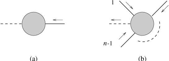
Figure 7: (a) Retarded self-energy, (b) generalized retarded $n$-point vertex functions.

We now discuss the $\hbar\rightarrow 0$ limit of these real-time quantum Feynman rules. This limit affects the diagrams in two ways. The first one is obvious, the thermal propagator $F_{0}$ has to be replaced by $S_{0}$. The second change leads to a drastic simplification: only the vertices (a) and (c) in fig. 6 contribute in the classical limit, and the two other vertices (b) and (d) can be neglected. This can be seen as follows: vertices (b) and (d) can only appear in a diagram with retarded (or advanced) Green functions attached to the three dashed legs. After attaching these Green functions, the resulting outer lines (which either still have to be attached to another vertex or are external lines) are always full lines. However, such a configuration can be constructed as well with vertices (a) and (c): these vertices have two full legs where (b) resp. (d) have two dashed legs. By attaching two thermal two-point functions on these legs, the external lines are full as well, and the vertices can be part of a diagram in exactly the same manner. But a classical thermal two-point function is proportional to $1/\hbar$. Diagrams with vertex (a) or (c) have two more thermal two-point functions than the corresponding diagrams with vertex (b) or (d). Hence, the first class of diagrams is relatively stronger in the classical limit with respect to the second class by a factor $1/\hbar^{2}$. In other words, vertices (b) and (d) will be ${\cal O}(\hbar^{2})$ suppressed with respect to vertices (a) and (c).

We propose that classical Feynman rules follow from the quantum ones by taking $\hbar$ to zero, which results in the following (simple) rules:

1. Draw all diagrams as in the quantum case, but use only vertices (a) and (c).

2. Replace the thermal propagator $F_{0}$ by its classical counterpart $S_{0}$.

An explicit check of these rules (by a comparison with the results obtained by perturbatively solving the equations of motion and averaging over the initial conditions) can be found for the case of $\lambda\phi^{4}$-theory for the two-point function up to two loops and the four-point function to one loop in [7].

A.2 Gauge invariant cut-off in the classical theory

We argue that in classical gauge theories it is possible to introduce a (continuum) momentum cut-off without breaking gauge invariance. The basic ingredient is the result of Landshoff and Rebhan [30] that in general linear gauges it is possible to formulate a (quantum) real-time theory in which only the two physical degrees of freedom of the gauge field acquire a thermal part. This implies that a change in the distribution function

$$n(k^{0})\rightarrow n(k^{0})f(k/\Lambda),$$ (A.15)

with $f$ some function, does not break gauge invariance. Introducing a cut-off in this way will not affect the Slavnov-Taylor identities. This has been employed in a Wilson renormalization group approach to hot (quantum) SU($N$) gauge theories [46].

If we take the classical limit of (A.15) and choose $f$ as the step function, we get

$$n_{\rm cl}(k^{0})\rightarrow n_{\rm cl}(k^{0})\theta(\Lambda-k),$$ (A.16)

which as (A.15) does not break gauge invariance. It is for instance straightforward to check that the HTL’s calculated with distribution function (A.16) satisfy the same abelian-like Ward identities as usual. Finally we should remark that the regularization (A.16) is sufficient to render the theory ultraviolet finite, since each loop introduces one distribution function.

Appendix B Classical one-loop SU($N$) self-energy: explicit calculation

We present in this appendix the calculation of the classical self-energy in SU($N$) gauge theory, in particular the $\Pi_{ii}$ part, in the Feynman gauge. The starting point is given by (LABEL:onels-e) in the main text. After changing variables from ${\mathbf{k}}\to-{\mathbf{k}}-{\mathbf{p}}$ in the part that is proportional to $n_{\rm cl}(\omega_{{\mathbf{p}}+{\mathbf{k}}})$, we find

$$\Pi_{ii,\rm cl}^{ab}(P)=\delta^{ab}g^{2}N\Pi_{\rm cl}(P),$$ (B.1)

with

$$\Pi_{\rm cl}(P)=\int\frac{d^{3}k}{(2\pi)^{3}}\,\frac{\hbar n_{\rm cl}(\omega_{{\mathbf{k}}})}{\omega_{{\mathbf{k}}}}\left\{6+\frac{A_{ii}}{(p^{0}+\omega_{{\mathbf{k}}})^{2}-\omega_{{\mathbf{p}}+{\mathbf{k}}}^{2}}+\frac{A_{ii}}{(p^{0}-\omega_{{\mathbf{k}}})^{2}-\omega_{{\mathbf{p}}+{\mathbf{k}}}^{2}}\right\},$$ (B.2)

and $A_{ii}=4k^{2}+4{\mathbf{k}}\cdot{\mathbf{p}}+5p^{2}-6p_{0}^{2}$. We have combined $\hbar$ with $n_{\rm cl}(\omega_{{\mathbf{k}}})$, which is an $\hbar$-independent combination.

The angular integrations can be performed, and

$$\Pi_{\rm cl}(p^{0},p)=\int dk\,\frac{k\hbar n_{\rm cl}(k)}{\pi^{2}}\bigg{\{}1+\frac{p^{0}}{p}\ln\frac{p_{+}}{p_{-}}-\frac{k}{2p}\Big{[}L_{+}(k)-L_{-}(k)\Big{]}\bigg{\}}$$

$$\;\;\;\;\;\;\;\;-\int dk\,\frac{k\hbar n_{\rm cl}(k)}{8\pi^{2}p}\bigg{\{}\frac{3p^{2}-4p_{0}^{2}}{k}\Big{[}L_{+}(k)-L_{-}(k)\Big{]}+4p^{0}\Big{[}L_{+}(k)+L_{-}(k)\Big{]}\bigg{\}}.$$

Motivated by Weldon [29], we used here the notation

$$p_{\pm}=\frac{1}{2}(p^{0}\pm p),\;\;\;\;L_{\pm}(k)=\ln\frac{k\pm p_{+}}{k\pm p_{-}}.$$ (B.4)

The result (B) agrees with the expression obtained by Weldon in the appendix of [29], except of course that the distribution function is classical in our case.

The remaining radial integral in the first line of (B) is linearly divergent. For the first two terms this is obvious, and for the third term one can use $L_{+}(k)-L_{-}(k)=2p/k+{\cal O}(k^{-3})$. In fact, the divergence in this term cancels against the first term. The integrals in the second line are convergent. To regulate the divergences, we use the distribution function with a momentum cut-off $\hbar n_{\rm cl}(k)=T/k\;\theta(\Lambda-k)$. The final result requires the evaluation of four integrals, which read (recall that $p^{0}$ contains a small positive imaginary part)

$$\int dk\,k\hbar n_{\rm cl}(k)=T\Lambda,$$ (B.5)

$$\int dk\,k^{2}\hbar n_{\rm cl}(k)\Big{[}L_{+}(k)-L_{-}(k)\Big{]}=T\left(2p\Lambda+\frac{1}{2}\pi ipp^{0}\right),$$ (B.6)

$$\int dk\,\hbar n_{\rm cl}(k)\Big{[}L_{+}(k)-L_{-}(k)\Big{]}=T\pi i\ln\frac{p_{+}}{p_{-}},$$ (B.7)

$$\int dk\,k\hbar n_{\rm cl}(k)\Big{[}L_{+}(k)+L_{-}(k)\Big{]}=-T\pi ip.$$ (B.8)

The second and fourth integral are straightforward using partial integration, and the third one can be performed by complex contour integration while being careful around $k=0$. Note that these integrals are much simpler than in the quantum case, because of the simple $k$ dependence of the classical distribution function.

Putting all the results together, we find for the classical one-loop retarded self energy

$$\Pi_{ii,\rm cl}^{ab}(P)=N\delta^{ab}g^{2}\left[\frac{T\Lambda}{\pi^{2}}\frac{p^{0}}{p}\ln\frac{p_{+}}{p_{-}}+\frac{T}{4\pi}\bigg{(}ip^{0}-\frac{3p^{2}-4p_{0}^{2}}{2p}i\ln\frac{p_{+}}{p_{-}}\bigg{)}\right],$$ (B.9)

which is presented in (2.9).

Appendix C Two loop naively linear divergent contributions

C.1 Diagram b

In this appendix we give the results for the naively linearly divergent contributions to the classical two-loop self-energy. We start with the classical limit of the self-energy diagram (b) in fig. 1, presented in (3.5), and use the shorthand notation of (3.6). There are three naively linearly divergent contributions and we shall denote these with (b1), (b2), and (b3).

We start with contribution (b1), obtained by taking $s_{3}=s^{\prime},s_{2}=-s$ and setting the external $p^{0},{\mathbf{p}}$ to zero in the energy denominators with three loop-energies. We then find

$$\Pi^{\rm(b1)}_{ij,\rm cl}(P)=\frac{1}{2}(g^{2}\hbar)^{2}\int\frac{d^{3}k}{(2\pi)^{3}}\int\frac{d^{3}k^{\prime}}{(2\pi)^{3}}(k)^{4}_{ij}\sum_{ss^{\prime}s_{1}}\frac{-s_{1}}{2^{5}\omega\omega^{\prime}\omega_{1}\omega_{2}\omega_{3}}\,\frac{1}{p^{0}+s^{\prime}(\omega^{\prime}+\omega_{3})}$$

$$\hskip 14.22636pt\frac{n_{\rm cl}(s\omega_{2})-n_{\rm cl}(s\omega)}{p^{0}+s(\omega-\omega_{2})}\,\left[\frac{n_{\rm cl}(s_{1}\omega_{1})-n_{\rm cl}(s^{\prime}\omega_{3})}{-s^{\prime}\omega^{\prime}-s\omega+s_{1}\omega_{1}}-\frac{n_{\rm cl}(s_{1}\omega_{1})+n_{\rm cl}(s^{\prime}\omega^{\prime})}{s^{\prime}\omega^{\prime}-s\omega+s_{1}\omega_{1}}\right].$$ (C.1)

The difference between distribution functions $\left[n_{\rm cl}(s\omega_{{\mathbf{p}}-{\mathbf{k}}})-n_{\rm cl}(s\omega_{{\mathbf{k}}})\right]$ reduces the degree of divergence by one compared to the naive estimate, which is from linear to logarithmic. Note that the other difference between distribution functions $\left[n_{\rm cl}(s_{1}\omega_{{\mathbf{k}}-{\mathbf{k}}^{\prime}})-n_{\rm cl}(s^{\prime}\omega_{{\mathbf{p}}-{\mathbf{k}}^{\prime}})\right]$, does not reduce the degree of divergence any further, since ${\mathbf{k}}$ is not a (small) external momentum, but is integrated over.

A similar contribution is obtained by taking $s_{2}=s$ and $s_{3}=-s^{\prime}$ and again setting $p^{0},{\mathbf{p}}=0$ in the same energy denominators. We obtain

$$\Pi^{\rm(b2)}_{ij,\rm cl}(P)=\frac{1}{2}(g^{2}\hbar)^{2}\int\frac{d^{3}k}{(2\pi)^{3}}\int\frac{d^{3}k^{\prime}}{(2\pi)^{3}}\,(k)^{4}_{ij}\sum_{ss^{\prime}s_{1}}\frac{-s_{1}}{2^{5}\omega\omega^{\prime}\omega_{1}\omega_{2}\omega_{3}}\,\frac{1}{p^{0}+s^{\prime}(\omega^{\prime}-\omega_{3})}$$

$$\hskip 14.22636pt\frac{n_{\rm cl}(s^{\prime}\omega_{3})-n_{\rm cl}(s^{\prime}\omega^{\prime})}{p^{0}+s(\omega+\omega_{2})}\left[-\frac{n_{\rm cl}(s_{1}\omega_{1})+n_{\rm cl}(s\omega_{2})}{s^{\prime}\omega^{\prime}+s\omega+s_{1}\omega_{1}}+\frac{n_{\rm cl}(s_{1}\omega_{1})-n_{\rm cl}(s\omega)}{s^{\prime}\omega^{\prime}-s\omega+s_{1}\omega_{1}}\right].$$ (C.2)

Again a difference between distribution functions appears that reduces the degree of divergence to a logarithmic one.

The third naively linearly divergent contribution to consider is of a different type. It is obtained from the classical limit of (3.5) by setting $s=-s_{2}$ and $s^{\prime}=-s_{3}$ and taking the linear term in $p^{0},{\mathbf{p}}$ in an expansion of the energy denominator with $\omega_{1}=\omega_{{\mathbf{k}}-{\mathbf{k}}^{\prime}}$. The zeroth order term in this expansion gives rise to a naively quadratic divergence and was already discussed in the main text. The first-order term reads

$$\Pi^{\rm(b3)}_{ij,\rm cl}(P)\!\!\!\! = \!\!\!\!\frac{1}{2}(g^{2}\hbar)^{2}\int\frac{d^{3}k}{(2\pi)^{3}}\int\frac{d^{3}k^{\prime}}{(2\pi)^{3}}\,(k)^{4}_{ij}\sum_{ss^{\prime}s_{1}}\frac{-s_{1}}{2^{5}\omega\omega^{\prime}\omega_{1}\omega_{2}\omega_{3}}\,$$ (C.3)

$$\!\!\!\!\frac{1}{p^{0}+s^{\prime}(\omega^{\prime}-\omega_{3})}\,\frac{1}{p^{0}+s(\omega-\omega_{2})}\,\frac{1}{\left(s^{\prime}\omega^{\prime}-s\omega+s_{1}\omega_{1}\right)^{2}}$$

$$\!\!\!\!\bigg{\{}s^{\prime}({\mathbf{p}}\cdot{\bf\hat{k}}^{\prime})\left[n_{\rm cl}(s\omega_{2})-n_{\rm cl}(s\omega)\right]\left[n_{\rm cl}(s^{\prime}\omega_{3})+n_{\rm cl}(s_{1}\omega_{1})\right]$$

$$-s({\mathbf{p}}\cdot{\bf\hat{k}})\left[n_{\rm cl}(s^{\prime}\omega_{3})-n_{\rm cl}(s^{\prime}\omega^{\prime})\right]\left[n_{\rm cl}(s\omega_{2})-n_{\rm cl}(s_{1}\omega_{1})\right]$$

$$+p^{0}n_{\rm cl}(s_{1}\omega_{1})\Big{(}[n_{\rm cl}(s\omega)-n_{\rm cl}(s\omega_{2})]+[n_{\rm cl}(s^{\prime}\omega^{\prime})-n_{\rm cl}(s^{\prime}\omega_{3})]\Big{)}$$

$$+p^{0}n_{\rm cl}(s_{1}\omega_{1})\left[n_{\rm cl}(s\omega)n_{\rm cl}(s^{\prime}\omega_{3})-n_{\rm cl}(s\omega_{2})n_{\rm cl}(s^{\prime}\omega^{\prime})\right]\bigg{\}}.$$

We emphasize again that the region of phase space where $s^{\prime}\omega^{\prime}-s\omega+s_{1}\omega_{1}$ vanishes is excluded in this expansion. The first three terms between curly brackets all have a factor which is the difference between distribution functions. The fourth term is different, but also here the factor with distribution functions vanishes when the external momentum is taken to zero (i.e. when $\omega_{2}\to\omega,\omega_{3}\to\omega^{\prime}$). Hence this factor contributes a power $\Lambda^{-3}$ instead of $\Lambda^{-2}$, and it brings down the degree of divergence. We conclude that the degree of divergence is reduced from linear to logarithmic in contribution (b3) as well.

C.2 Diagram c

The final diagram that needs to be examined is diagram (c) in fig. 1. The quantum expression is

$$\Pi^{\rm(c)}_{ij}(P)=(g^{2}\hbar)^{2}\int\frac{d^{3}k}{(2\pi)^{3}}\int\frac{d^{3}k^{\prime}}{(2\pi)^{3}}\,(k)^{2}_{ij}\sum_{ss^{\prime}s_{1}s_{2}}\frac{ss^{\prime}s_{1}s_{2}}{2^{4}\omega\omega^{\prime}\omega_{1}\omega_{2}}\,\frac{1}{p^{0}-s\omega-s_{2}\omega_{2}}$$

$$\hskip 68.28644pt\bigg{\{}\frac{1}{s\omega+s^{\prime}\omega^{\prime}-s_{1}\omega_{1}}\Big{(}[n(s\omega)+1][n(s^{\prime}\omega^{\prime})+1]n(s_{1}\omega_{1})$$

$$\hskip 108.12054pt-n(s\omega)n(s^{\prime}\omega^{\prime})[n(s_{1}\omega_{1})+1]\Big{)}$$

$$\hskip 68.28644pt+\frac{1}{p^{0}-s_{2}\omega_{2}+s^{\prime}\omega^{\prime}-s_{1}\omega_{1}}\Big{(}[n(s^{\prime}\omega^{\prime})+1]n(s_{1}\omega_{1})n(s_{2}\omega_{2})-$$

$$\hskip 108.12054ptn(s^{\prime}\omega^{\prime})[n(s_{1}\omega_{1})+1][n(s_{2}\omega_{2})+1]\Big{)}\bigg{\}},$$ (C.4)

where in this case $\omega_{1}=\omega_{{\mathbf{p}}-{\mathbf{k}}-{\mathbf{k}}^{\prime}}$ and we inserted $(k)^{2}_{ij}$ to indicate the two powers of momentum that come from the two three-point vertices.

We take the classical limit of (C.4). The contribution with $s_{2}=-s$ is naively linearly divergent, it reads

$$\tilde{\Pi}^{\rm(c)}_{ij,\rm cl}=(g^{2}\hbar)^{2}\int\frac{d^{3}k}{(2\pi)^{3}}\int\frac{d^{3}k^{\prime}}{(2\pi)^{3}}\,(k)^{2}_{ij}\sum_{ss^{\prime}s_{1}}\frac{-s^{\prime}s_{1}}{2^{4}\omega\omega^{\prime}\omega_{1}\omega_{2}}\,\frac{1}{p^{0}-s\omega+s\omega^{\prime}}$$

$$\hskip 28.45274pt\frac{1}{s\omega+s^{\prime}\omega^{\prime}-s_{1}\omega_{{\mathbf{k}}+{\mathbf{k}}^{\prime}}}\,[n(s\omega)-n(s\omega_{2})][n(s_{1}\omega_{1})-n(s^{\prime}\omega^{\prime})].$$ (C.5)

Again the first difference between distribution functions reduces the degree of divergence to a logarithmic one.

References

- [1] D. Y. Grigoriev and V. A. Rubakov, Nucl. Phys. B299 (1988) 67; D. Y. Grigoriev, V. A. Rubakov, and M. E. Shaposhnikov, Phys. Lett. B216 (1989) 172.
- [2] For recent reviews, see J. Smit, Nucl. Phys. Proc. Suppl. 63 (1998) 89, hep-lat/9710026; G. D. Moore, in Lattice ’99, Pisa, Italy, 1999, hep-lat/9907009.
- [3] D. Bödeker, L. McLerran, and A. Smilga, Phys. Rev. D52 (1995) 4675, hep-th/9504123.
- [4] P. Arnold, D. Son, and L. G. Yaffe, Phys. Rev. D55 (1997) 6264, hep-ph/9609481.
- [5] P. Arnold, Phys. Rev. D55 (1997) 7781, hep-ph/9701393.
- [6] G. Aarts and J. Smit, Phys. Lett. B393 (1997) 395, hep-ph/9610415.
- [7] G. Aarts and J. Smit, Nucl. Phys. B511 (1998) 451, hep-ph/9707342.
- [8] W. Buchmüller and A. Jakovác, Phys. Lett. B407 (1997) 39, hep-ph/9705452.
- [9] B. J. Nauta and C. G. van Weert, Phys. Lett. B444 (1998) 463, hep-ph/9709401; hep-ph/9901213.
- [10] J. Ambjørn and A. Krasnitz, Phys. Lett. B362 (1995) 97, hep-ph/9508202; Nucl. Phys. B506 (1997) 387, hep-ph/9705380.
- [11] G. D. Moore and N. Turok, Phys. Rev. D56 (1997) 6533, hep-ph/9703266; G. D. Moore, Nucl. Phys. B480 (1996) 657, hep-ph/9603384; G. D. Moore and K. Rummukainen, hep-ph/9906259.
- [12] W. H. Tang and J. Smit, Nucl. Phys. B482 (1996) 265, hep-lat/9605016.
- [13] For recent reviews, see e.g. V. A. Rubakov and M. E. Shaposhnikov, Usp. Fiz. Nauk 166 (1996) 493, hep-ph/9603208; M. Trodden, hep-ph/9803479.
- [14] G. D. Moore and N. Turok, Phys. Rev. D55 (1997) 6538, hep-ph/9608350.
- [15] W. H. Tang and J. Smit, Nucl. Phys. B510 (1998) 401, hep-lat/9702017.
- [16] E. Braaten and R. D. Pisarski, Nucl. Phys. B337 (1990) 569.
- [17] J. C. Taylor and S. M. H. Wong, Nucl. Phys. B346 (1990) 115.
- [18] M. Le Bellac, Thermal Field Theory, Cambridge University Press, 1996.
- [19] C. R. Hu and B. Müller, Phys. Lett. B409 (1997) 377, hep-ph/9611292.
- [20] E. Iancu, Phys. Lett. B435 (1998) 152, hep-ph/9710543.
- [21] G. D. Moore, C. R. Hu, and B. Müller, Phys. Rev. D58 (1998) 045001, hep-ph/9710436.
- [22] A. Rajantie and M. Hindmarsh, Phys. Rev. D60 (1999) 096001, hep-ph/9904270.
- [23] D. Bödeker, G. D. Moore, and K. Rummukainen, hep-ph/9907545.
- [24] D. Bödeker, Phys. Lett. B426 (1998) 351, hep-ph/9801430.
- [25] P. Arnold, D. T. Son, and L. G. Yaffe, Phys. Rev. D59 (1999) 105020, hep-ph/9810216.
- [26] G. D. Moore, hep-ph/9810313.
- [27] D. F. Litim and C. Manuel, Phys. Rev. Lett. 82 (1999) 4981, hep-ph/9902430; hep-ph/9906210.
- [28] V. Silin, Sov. Phys. JETP 11 (1960) 1136.
- [29] H. A. Weldon, Phys. Rev. D26 (1982) 1394.
- [30] P. V. Landshoff and A. Rebhan, Nucl. Phys. B383 (1992) 607, hep-ph/9205235; Nucl. Phys. B410 (1993) 23, hep-ph/9303276.
- [31] B. J. Nauta, hep-ph/9906389.
- [32] F. T. Brandt, J. Frenkel, and J. C. Taylor, Phys. Rev. D44 (1991) 1801.
- [33] K. Kajantie and J. Kapusta, Ann. Phys. 160 (1985) 477.
- [34] F. Guérin, Phys. Rev. D49 (1994) 4182.
- [35] M. van Eijck, Thermal field theory and the finite-temperature renormalization group, thesis, University of Amsterdam (1995), Ch. 2, 3.
- [36] J. I. Kapusta, Finite-Temperature Field Theory, Cambridge University Press, 1989.
- [37] P. Arnold and C.-X. Zhai, Phys. Rev. D50 (1994) 7603, hep-ph/9408276.
- [38] A. Jakovác, Phys. Lett. B446 (1999) 203, hep-ph/9808349.
- [39] S. Jeon, Phys. Rev. D52 (1995) 3591, hep-ph/9409250.
- [40] J.P. Blaizot and E. Iancu, Nucl. Phys. B417 (1994) 608, hep-ph/9306294; Nucl. Phys. B421 (1994) 565, hep-ph/9401211.
- [41] K. Kajantie, M. Laine, K. Rummukainen, and M. Shaposhnikov, Nucl. Phys. B458 (1996) 90, hep-ph/9508379.
- [42] G. Aarts, in proceedings of Strong and Electroweak Matter (SEWM 97), Eger, Hungary, 21-25 May 1997, 267, hep-ph/9707440.
- [43] G. Parisi, Statistical Field Theory, Addison-Wesley Publishing Company, 1988.
- [44] J. Schwinger, J. Math. Phys. 2 (1961) 407; L. V. Keldysh, Zh. Eksp. Teor. Fiz. 47 (1964) 1515 [Sov. Phys. JETP 20 (1965) 1018]; N. P. Landsman and C. G. van Weert, Phys. Rept. 145 (1987) 141.
- [45] M. A. van Eijck, R. Kobes, and Ch. G. van Weert, Phys. Rev. D50 (1994) 4097, hep-ph/9406214.
- [46] M. D’Attanasio and M. Pietroni, Nucl. Phys. B498 (1997) 443, hep-th/9611038; D. Comelli and M. Pietroni, Phys. Lett. B417 (1998) 337, hep-ph/9708489.