hep-ph/9911459 ACT-12/99 CERN-TH/99-237 CTP-TAMU-45/99 FISIST/22-99/CFIF Charged-Lepton-Flavour Violation in the Light of the Super-Kamiokande Data

Motivated by the data from Super-Kamiokande and elsewhere indicating oscillations of atmospheric and solar neutrinos, we study charged-lepton-flavour violation, in particular the radiative decays $\mu\rightarrow e\gamma$ and $\tau\rightarrow\mu\gamma$, but also commenting on $\mu\rightarrow 3e$ and $\tau\to 3\mu/e$ decays, as well as $\mu\to e$ conversion on nuclei. We first show how the renormalization group may be used to calculate flavour-violating soft supersymmetry-breaking masses for charged sleptons and sneutrinos in models with universal input parameters. Subsequently, we classify possible patterns of lepton-flavour violation in the context of phenomenological neutrino mass textures that accommodate the Super-Kamiokande data, giving examples based on Abelian flavour symmetries. Then we calculate in these examples rates for $\mu\rightarrow e\gamma$ and $\tau\rightarrow\mu\gamma$, which may be close to the present experimental upper limits, and show how they may distinguish between the different generic mixing patterns. The rates are promisingly large when the soft supersymmetry-breaking mass parameters are chosen to be consistent with the cosmological relic-density constraints. In addition, we discuss $\mu\rightarrow e$ conversion on Titanium, which may also be accessible to future experiments.

November 1999

 

1. Introduction

There has been increasing interest in massive neutrinos during the past year, triggered principally by the Super-Kamiokande data [1] on the $\nu_{\mu}/\nu_{e}$ ratio in the atmosphere. The latter was found to be significantly smaller than the Standard Model expectations, with a characteristic azimuthal-angle dependence indicating the presence of neutrino oscillations. The data analysis favours $\nu_{\mu}\to\nu_{\tau}$ oscillations, with parameters in the ranges

$$\delta m_{\nu_{\mu}\nu_{\tau}}^{2} \sim (10^{-2}\;{\rm to}\;10^{-3})\;{\rm eV^{2}}$$ (1)

$$\sin^{2}2\theta_{\mu\tau} \geq 0.8$$ (2)

Dominance by $\nu_{\mu}\rightarrow\nu_{e}$ oscillations is disfavoured by the Super-Kamiokande data on electron-like events [1], as well as by the data from the Chooz reactor experiment [2]. Oscillations involving a sterile neutrino are disfavoured, but not yet excluded, by a detailed study of the azimuthal-angle dependence of muon-like events [1] and by measurements of $\pi^{0}$ production. Moreover, in most theoretical models sterile neutrinos tend to be heavy. Therefore, we consider $\nu_{\mu}\rightarrow\nu_{\tau}$ as the ‘established’ hypothesis for the atmospheric neutrino data.

In addition, the long-standing deficit of solar $\nu_{e}$ measured on Earth may also be explained via neutrino oscillations, either in vacuo or enhanced in matter by the Mikheyev-Smirnov-Wolfenstein (MSW) mechanism [3]. The first option would require $\delta m_{\nu_{e}\nu_{\alpha}}^{2}\sim(0.5-1.1)\times 10^{-10}~{}{\rm eV}^{2}$, where $\alpha$ is $\mu$ or $\tau$. MSW oscillations [3], on the other hand, require $\delta m_{\nu_{e}\nu_{\alpha}}^{2}\sim(0.3-20)\times 10^{-5}~{}{\rm eV}^{2}$ with either large $\sin^{2}2\theta_{e\alpha}\sim 1$ or small $\sin^{2}2\theta_{e\alpha}\sim 10^{-2}$. The presence of either $\nu_{e}\rightarrow\nu_{\mu}$ or $\nu_{e}\rightarrow\nu_{\tau}$ oscillations at a high level is, therefore, an open question.

Both the solar and atmospheric neutrino data can be accommodated in a natural way in schemes with three light neutrinos with at least one large mixing angle and hierarchical masses, of the order of the required mass differences: $m_{3}\sim(10^{-1}\;{\rm to}\;10^{-1.5})$ eV and $m_{2}\sim(10^{-2}\;{\rm to}\;10^{-3})$ eV $\gg m_{3}$. On the other hand, if neutrinos were also to provide significant hot dark matter, three almost-degenerate neutrinos with masses of $\approx 1$ eV would be needed.

Neutrino oscillations involve violations of the individual lepton numbers $L_{e,\mu,\tau}$, raising the prospect that there might also exist observable processes that violate charged-lepton number conservation [4, 5], such as $\mu\rightarrow e\gamma,3e$ and $\tau\rightarrow\mu\gamma,3\mu/e$, and $\mu\to e$ conversion on heavy nuclei [5, 6, 7, 8, 9, 10]. We recall briefly the present experimental upper limits on the most interesting of these decays for our subsequent discussion:

$$BR(\mu\rightarrow e\gamma)\,<\,1.2\times 10^{-11}\, :$$ [11] (3)

$$BR(\mu^{+}\rightarrow e^{+}e^{+}e^{-})\,<\,1.0\times 10^{-12}\, :$$ [12] (4)

$$R(\mu^{-}Ti\rightarrow e^{-}Ti)\,<\,6.1\times 10^{-13}\, :$$ [13] (5)

$$BR(\tau\rightarrow\mu\gamma)\,<1.1\times\,10^{-6}\, :$$ [14] (6)

Projects are currently underway to improve several of these upper limits significantly:

$$BR(\mu\rightarrow e\gamma)\,\rightarrow\,10^{-14}\, :$$ [15] (7)

$$R(\mu^{-}Ti\rightarrow e^{-}Ti)\,\rightarrow\,{\rm few}\times 10^{-14}\, :$$ [16] (8)

$$R(\mu^{-}Al\rightarrow e^{-}Al)\,\rightarrow\,1\times 10^{-16}\, :$$ [17] (9)

$$BR(\tau\rightarrow\mu\gamma)\,\rightarrow 1\times\,10^{-9}~{}?\, :$$ [18] (10)

and there are active discussions of intense $\mu$ sources that might enable the upper limits on $\mu\rightarrow e$ transitions to be improved by several further orders of magnitude [19].

We evaluate the possibility of charged-lepton-flavour violation using the most natural mechanism for obtaining neutrino masses in the sub-eV range, namely the see-saw mechanism [20], which involves Dirac neutrino masses $m_{\nu}^{D}$ of the same order as the charged-lepton and quark masses, and heavy Majorana masses $M_{\nu_{R}}$, leading to light effective neutrino mass matrices:

$$m_{eff}=m^{D}_{\nu}\cdot(M_{\nu_{R}})^{-1}\cdot m^{D^{\normalsize T}}_{\nu}.$$ (11)

Neutrino-flavour mixing may then occur through either the Dirac and/or the Majorana mass matrices, which may also feed flavour violation through to the charged leptons.

The specific mechanism explored in this paper is renormalization of the sneutrino and slepton masses in a supersymmetric theory via the neutrino Dirac couplings $\lambda^{D}_{\nu}$ [5]. It is well known that the prototypical charged-lepton flavour-violating process $\mu\to e\gamma$ provides one of the most stringent upper limits on flavour violation in the Minimal Supersymmetric extension of the Standard Model (MSSM). If the soft supersymmetry-breaking sneutrino and slepton masses were non-universal before renormalization, it would be very difficult to understand why this decay was not seen long ago. Universal scalar masses arise naturally in no-scale supergravity models [21], the framework favoured here, as well as in gauge-mediated models [22]. In the universal supergravity case, the soft supersymmetry-breaking sneutrino and slepton masses are subject to calculable and non-trivial renormalization via Dirac neutrino couplings at scales between $M_{GUT}\sim 10^{16}$ GeV and $M_{\nu_{R}}\sim 10^{13}$ GeV.

The predictions of this class of universal supergravity models are quite characteristic. In non-supersymmetric models with massive neutrinos, the amplitudes for the charged-lepton-flavour violation are proportional to inverse powers of the right-handed neutrino mass scale $M_{\nu_{R}}$ [4]. Since the latter is much higher than the electroweak scale, the rates for rare decays such as $\mu\to e\gamma$ are extremely suppressed [4]. On the other hand, in supersymmetric models these processes are only suppressed by inverse powers of the supersymmetry breaking scale, which is at most $1$ TeV [5]. Among such models, those with non-universal input scalar masses at the GUT scale generally predict excessive rates for rare charged-lepton-flavour violation, whereas they are very suppressed in no-scale [21] and gauge-mediated models [22]. The class of supergravity models with universal scalar masses that we consider here toe the fine line between excessive and unobservable charged-lepton-flavour violation, as we discuss in more detail below.

Here we re-analyze the prospects for charged-lepton-flavour violation in this theoretical framework, using as a guide the indications from Super-Kamiokande and elsewhere on neutrino masses and mixing. Within the general see-saw scenario, solutions with various differences in the neutrino mass-matrix structure have been proposed, including models with maximal [23, 24], close-to-maximal [25, 26] and bi-maximal [27] neutrino mixing. In the following, we categorize models according to whether the off-diagonal elements in their Dirac and Majorana couplings ‘match’ in such a way that their mixing is almost two-generational (and hence predominantly in the $\mu-\tau$ sector), and more general models in which they ‘mismatch’, and the mixing is essentially three-generational (and substantial also in the $\mu-e$ and $\tau-e$ sectors). We provide examples of the ‘matched’ and ‘mismatched’ categories in schemes with Abelian [28, 25, 26] flavour symmetries, and comment on the possibilities with non-Abelian [29] flavour symmetries, as well as in a string-derived flipped $SU(5)$ model [30], whose characteristic property is the appearance of large off-diagonal $\mu-e$ couplings in the Dirac neutrino-mass matrix [24]. As we exemplify with calculations in the Abelian models, the rates for the radiative decays $\mu\to e\gamma$ and $\tau\to\mu\gamma$ may offer good prospects for testing different textures. These decays may well take place at observable rates, and different neutrino-mass models correlate their decay rates in characteristically different ways, enabling $\mu\to e\gamma$ and $\tau\to\mu\gamma$ to serve as useful diagnostic tools for neutrino-mass models. Finally, we calculate in some models the rate for $\mu\to e$ conversion on Titanium, which may also be accessible to future experiments, and comment briefly on $\mu\to 3e$ decay.

2. General Aspects of Charged-Lepton-Flavour Violation in Supersymmetric Models with Universal Breaking

We first display in Fig. 1 the one-loop diagrams that give rise to $\mu\rightarrow e\gamma$, noting that the $\tau\rightarrow\mu\gamma$-decay is generated by an analogous set of graphs. We later extend the discussion to include $\mu\rightarrow 3e$ decay, $\tau\rightarrow 3\mu/e$ and $\mu\rightarrow e$ conversion. The matrix element of the electromagnetic-current operator between two distinct lepton states $l_{i}$ and $l_{j}$ is given in general by

$${\cal T}_{\lambda} = \langle l_{i}|(p-q)|{\cal J}_{\lambda}|l_{j}(p)\rangle$$ (12)

$$= {\bar{u}_{i}}(p-q)\{m_{j}i\sigma_{\lambda\beta}q^{\beta}\left(A^{L}_{M}P_{L}+A^{R}_{M}P_{R}\right)+$$

$$\quad\quad(q^{2}\gamma_{\lambda}-q_{\lambda}\gamma\cdot q)\left(A^{L}_{E}P_{L}+A^{R}_{E}P_{R}\right)\}u_{j}(p)$$

where $q$ is the photon momentum. The coefficients $A_{M}$ and $A_{E}$ receive contributions from both neutralino (n)/charged-slepton (Fig. 1(a)) and chargino (c)/sneutrino (Fig. 1(b) exchanges:

$$A_{M}^{L,R}=A_{M(n)}^{L,R}+A_{M(c)}^{L,R},\quad A_{E}^{L,R}=A_{E(n)}^{L,R}+A_{E(c)}^{L,R}$$ (13)

The amplitude of the process is then proportional to ${\cal T}_{\lambda}\epsilon^{\lambda}$, where $\epsilon^{\lambda}$ is the photon-polarization vector.

Figure 1: Generic Feynman diagrams for $\mu\rightarrow e\gamma$ decay: $\tilde{l}$ represents a charged slepton (a) or sneutrino (b), and $\tilde{\chi}^{(n)}$ and $\tilde{\chi}^{(c)}$ represent neutralinos and charginos respectively.

We recall that the easiest way to determine the loop momentum-integral contributions to the coefficients $A_{M,E}$ is to identify, in the corresponding diagram, terms proportional to $(p\cdot\epsilon)$ and $(q\cdot\epsilon)$. The coefficient of the former is proportional to the momentum-integral contribution to the $\sigma_{\lambda\beta}$ term in (12), while the coefficient of the latter is proportional to the difference between the momentum-integral contributions to the $\sigma_{\lambda\beta}$ and $(q^{2}\gamma_{\lambda}-q_{\lambda}\gamma\cdot q)$ terms. Defining $x\equiv M^{2}/m^{2}$, where $M$ is the chargino (neutralino) mass and $m$ the sneutrino (charged slepton) mass, the following functions appear in the $A_{M}$ terms [10, 5]:

$$\begin{array}[]{ll}A_{M(n)}:&\frac{1}{6(1-x)^{4}}(1-6x+3x^{2}+2x^{3}-6x^{2}\log x)\quad\hbox{and}\\ &\frac{1}{(1-x)^{3}}(1-x^{2}+2x\log x)\frac{M}{m_{l_{j}}}\\ A_{M(c)}:&\frac{1}{6(1-x)^{4}}(2+3x-6x^{2}+x^{3}+6x\log x)\quad\hbox{and}\\ &\frac{1}{(1-x)^{3}}(-3+4x-x^{2}-2\log x)\frac{M}{m_{l_{j}}}\end{array}$$ (14)

where $m_{l_{j}}$ is the mass of the $l_{j}$ lepton, while for the $A_{E}$ terms we have:

$$\begin{array}[]{ll}A_{E(n)}:&\frac{1}{(1-x)^{4}}(2-9x+18x^{2}-18x^{3}+6x^{3}\log x)\\ A_{E(c)}:&\frac{1}{(1-x)^{4}}(16-45x+36x^{2}-7x^{3}+6(2-3x)\log x).\end{array}$$ (15)

Note in this case the lack of terms proportional to the gaugino mass $M$. The branching ratio (BR) of the decay $l_{j}\rightarrow l_{i}+\gamma$ is then given by:

$$BR(l_{j}\rightarrow l_{i}\gamma)=\frac{48\pi^{3}\alpha}{G_{F}^{2}}\left((A_{M}^{L})^{2}+(A_{M}^{R})^{2}\right)$$ (16)

We see, therefore, that the branching ratios for radiative lepton decays involve the masses of several supersymmetric particles at low energies.

As stated in the Introduction, in this work we assume universal scalar masses and trilinear terms $A$ at the GUT scale. However, the physical values of these masses to be used in (14,15,16) have to be obtained by integrating the renormalization-group equations of the MSSM supplemented with right-handed neutrinos, found, for example, in [31]). The Dirac neutrino and charged lepton Yukawa couplings cannot, in general, be diagonalized simultaneously. Since both these sets of lepton Yukawa couplings appear in the renormalisation-group equations, the lepton Yukawa matrices and the slepton mass matrices can not be simultaneously diagonalized at low energies either. Indeed, in the basis where $m_{\ell}$ is diagonal, the slepton-mass matrix acquires non-diagonal contributions from renormalization at scales below $M_{GUT}$, of the form [5]:

$$\delta\tilde{m}_{\ell}^{2}\propto\frac{1}{16\pi^{2}}(3+a^{2})\ln\frac{M_{GUT}}{M_{N}}\lambda_{D}^{\dagger}\lambda_{D}m_{3/2}^{2},$$ (17)

where $\lambda_{D}$ is the Dirac neutrino Yukawa coupling, $M_{N}$ is the intermediate scale where the effective neutrino-mass operator is formed, and $a$ is related to the trilinear mass parameter: $A_{l}=am_{3/2}$, where $m_{3/2}^{2}$ is the common value of the scalar masses at the GUT scale. As a result, the diagrams of Fig. 1 lead to radiative decays of charged leptons .

We obtain the physical charged-slepton masses by numerical diagonalization of the following $6\times 6$ matrix:

$$\tilde{m}_{\ell}^{2}=\left(\begin{array}[]{cc}m_{LL}^{2}&m_{LR}^{2}\\ m_{RL}^{2}&m_{RR}^{2}\end{array}\right)$$ (18)

where all tha entries are $3\times 3$ matrices in flavour space. Using the superfield basis where $\lambda_{\ell}$ is diagonal, it is convenient for later use to write the $3\times 3$ entries of (18) in the form:

$$m_{LL}^{2} = (m_{\tilde{\ell}}^{\delta})^{2}+\delta m_{\nu_{D}}^{2}+m_{\ell}^{2}-M_{Z}^{2}(\frac{1}{2}-sin^{2}\theta_{W})cos2\beta$$ (19)

$$m_{RR}^{2} = (m_{\tilde{e_{R}}}^{\delta})^{2}+m_{\ell}^{2}-M_{Z}^{2}sin^{2}\theta_{W}cos2\beta$$ (20)

$$m_{RL}^{2} = (A_{e}^{\delta}+\delta A_{e}-\mu tan\beta)m_{\ell}$$ (21)

$$m_{LR}^{2} = m_{RL}^{2\dagger}$$ (22)

where $\tan\beta$ is the standard ratio of the two MSSM Higgs vevs, $(m_{\tilde{\ell}}^{\delta})^{2},(m_{\tilde{e_{R}}}^{\delta})^{2}$ and $A_{e}^{\delta}$ denote the diagonal contributions to the corresponding matrices, obtained by numerical integration of the renormalization-group equations, and $\delta m_{\nu_{D}}^{2}$ and $\delta A_{l}$ denote the off-diagonal terms that appear because $\lambda_{D}$ and $\lambda_{\ell}$ may not be diagonalized simultaneously (17).

The full mass matrix for left- and right-handed sneutrinos has a $12\times 12$ structure, given in terms of $3\times 3$ Dirac, Majorana and sneutrino mass matrices. The effective $3\times 3$ mass-squared matrix for the left-handed sneutrinos has the same form as the $m_{LL}^{2}$ part (22) of the $6\times 6$ charged-slepton matrix (18), with the difference that now the Dirac masses are absent. One might have expected that - as in the case of charged sleptons - the Dirac terms would induce considerable mixing effects. However, we show here that this is not the case in the sneutrino-mass matrix. Due to the vastly different scales involved in the full $12\times 12$ sneutrino mass matrix, a complete analysis is not straightforward. Instead, we construct an effective $6\times 6$ matrix for the light sector, by applying matrix perturbation theory, in analogy with to the see-saw mechanism [20]. To second order, the result is:

$$(m_{\tilde{\nu}}^{2})_{eff}=\left(\begin{array}[]{cc}m_{\tilde{\ell}}^{2}+{\cal O}(m_{\tilde{\ell}}^{4}M^{-2})&((2A_{\nu}+A_{N})-2\mu\cot\beta)\cdot\\ &\hskip 25.6073pt(m_{D}M^{-1}m_{D}^{\dagger})\\ &\\ ((2A_{\nu}+A_{N})-2\mu\cot\beta)\cdot&m_{\tilde{\ell}}^{2}+{\cal O}(m_{\tilde{\ell}}^{4}M^{-2})\\ \hskip 25.6073pt(m_{D}M^{-1}m_{D}^{\dagger})^{*}&\end{array}\right)$$ (23)

The first- and second-order terms in (23) are obtained assuming that all the parameters as real and the matrices $A_{\nu,N}$ are proportional to the identity. Notice that the second-order terms along the diagonal can be neglected, whereas the first-order off-diagonal terms must be retained, since they lead to complete mixing of the pair-wise degenerate states. However, this does not affect the branching ratios for the flavour-violating radiative decays. Therefore, we simply use [8]

$$\tilde{m}_{\nu}^{2}=(m_{\tilde{l}}^{\delta})^{2}+\delta m_{\nu_{D}}^{2}+\frac{1}{2}M_{Z}^{2}cos2\beta$$ (24)

in our subsequent calculations.

Next we consider the rare decay $\mu\rightarrow 3e$ and $\mu\rightarrow e$ conversion on nuclei, starting with the $\mu\rightarrow 3e$ reaction. This reaction is interesting on its own since it has a structure much richer than that of the $\mu\rightarrow e\gamma$ decay. Thus, it is possible that $\mu\rightarrow 3e$ can take place in cases where $\mu\rightarrow e\gamma$ is forbidden. This and the related $\tau\rightarrow 3\mu/e$ decay receive contributions from three types of Feynman diagrams. The first are photon ‘penguin’ diagrams related to the diagrams for $\mu\rightarrow e\gamma$ and $\tau\rightarrow\mu/e\gamma$ discussed above, where now the photon is virtual and decays into an $e^{+}e^{-}$ (or $\mu^{+}\mu^{-}$) pair. A second class of diagrams is obtained by replacing the photon line with a $Z$ boson. Finally, there are also box diagrams. In addition, all the above types of diagrams are accompanied by their supersymmetric analogues. We evaluate all the relevant diagrams exactly in our subsequent numerical analysis. However, we note that the dominant diagrams in the models of interest to us here are generally the ‘penguin’ diagrams with an intermediate off-shell photon, which contribute via the $A_{M}$ and $A_{E}$ terms presented in (14,15). Compared to $\mu\rightarrow e\gamma$ decay, the branching ratio is,

$${\Gamma(\mu^{+}\rightarrow e^{+}e^{+}e^{-})\over\Gamma(\mu^{+}\rightarrow e^{+}\gamma)}\approx 6\times 10^{-3}$$ (25)

This does not necessarily mean that $\mu\rightarrow 3e$ decay is uninteresting to experiment, because the experimental detection and background problems are very different for the two decays. However, we do not present detailed numerical results for $\mu^{+}\rightarrow e^{+}e^{+}e^{-}$ decay, because the factor (25) is essentially universal. There is a similar small ratio for $\tau\rightarrow 3\mu/e$ relative to $\tau\rightarrow\mu/e\gamma$, which seems to preclude its observation even at the LHC.

The $\mu\rightarrow e$ conversion is a coherent process in a muonic atom originally studied in [32, 33]. Even though this reaction proceeds via the same classes of diagrams as those discussed above in connection with $\mu^{+}\rightarrow e^{+}e^{+}e^{-}$, this reaction is rather different, since it involves hadronic currents. Effects of nuclear nature, such as the size of the nucleus in particular when heavy atoms are involved, play important role. Detailed calculations including all contributions from penguin and the box diagrams will be given in section 5. Here, in order to obtain a first rough estimate of the ratio of the $\mu\rightarrow e$ conversion to the $\mu\rightarrow e\gamma$ reaction, we restrict to the photonic contribution which dominates over a large portion of the parameter space. The $\mu\rightarrow e$ conversion rate relative to conventional muon capture, is given by

$$R(\mu\rightarrow e)\equiv\frac{\Gamma(\mu^{+}\rightarrow e^{+})}{\Gamma(\mu\rightarrow\nu_{\mu})} = (\frac{4\pi\alpha}{G_{F}})^{2}\frac{E_{e}p_{e}}{m_{\mu}^{2}}\frac{|ME|^{2}}{CZf(A,Z)}(|A^{L}+A^{R}|^{2}+|A^{L}-A^{R}|^{2})$$ (26)

where $A^{L/R}\equiv A^{L/R}_{M}+A^{L/R}_{E}$. It is important to note that the combination of matrix elements $A_{M/E}^{L/R}$ in (26) is different from that in appearing $\mu\rightarrow e$ decay (16). The function $f(A,Z)$ is given in [34], and has the following approximate value for elements with $A\approx 2Z$

$$f(A,Z)=1.0-0.03\frac{A}{2Z}+0.25\left(\frac{A}{2Z}-1\right)+3.24\left(\frac{Z}{2A}-\frac{1}{2}-\frac{1}{4A}|\frac{A}{2Z}-1|\right)\approx 0.16$$ (27)

Further, the parameter $C$ in (26) is [34]

$$C=|F_{V}^{2}+3F_{A}^{2}+F_{P}^{2}-2F_{A}F_{P}|\sim 5.9$$ (28)

and the nuclear matrix element $|ME|$ is

$$|ME|=|<(A,Z)_{f}|J(0)|(A,Z)_{i}>|\approx ZF_{c}(q^{2}),$$ (29)

where, in the case of the photonic diagram, $F_{c}(q^{2})$ stands for the proton or neutron form factor. Calculations using the nuclear shell model for ${}^{48}{}_{22}Ti$ have yielded $F_{c}(q^{2}=-m_{\mu}^{2})\approx 0.543$ for the case of proton and $0.528$ for the neutron [35, 36]. Comparing now with $B(\mu^{+}\rightarrow e^{+}\gamma)$, one obtains a rough estimate of the expected range of the $\mu\rightarrow e$ conversion ratio:

$$R({\mu^{+}Ti\rightarrow e^{+}Ti}) \approx \frac{\alpha}{3\pi}\frac{E_{e}p_{e}}{m_{\mu}^{2}}\frac{ZF_{c}^{2}}{Cf(A,Z)}BR(\mu\rightarrow e\gamma)$$ (30)

$$\approx 5.6\times 10^{-3}BR(\mu\rightarrow e\gamma)$$

which shows a relative suppression about two orders of magnitude. Nevertheless, $\mu\rightarrow e$ conversion is also interesting. Current experimental bounds give $R(\mu^{+}Ti\rightarrow e^{+}Ti)\leq 6.1\times 10^{-13}$, whilst ongoing experiments will reach $\sim 2\times 10^{-14}$. However, with an intense proton (and muon) source, such as that projected for a neutrino factory or a muon collider, experiments sensitive to rates as low as $10^{-16}$ may be feasible [19]. Moreover, as is apparent from (26) above, and the appearance of box diagrams, the structure of the matrix element is different from that for $\mu\rightarrow e\gamma$ (16), so the ratio (30) is not universal, unlike the $\mu\rightarrow 3e$ case. Therefore, although we emphasize $\mu\rightarrow e\gamma$ in what follows, we shall also present later some results for $\mu\rightarrow e$ conversion on Titanium.

3. Neutrino Mass Textures in the Light of Super-Kamiokande

Having discussed the theoretical framework for calculating charged-lepton-flavour violation in a supersymmetric model with universal input soft supersymmetry-breaking parameters at the GUT scale, we now discuss possible extreme patterns of neutrino masses, mixings and Yukawa couplings that might figure in the renormalization-group equations.

The most basic piece of information from the recent atmospheric-neutrino data is the existence of at least one large mixing angle in the lepton sector, that associated with the $\mu-\tau$ flavour mixing. Lepton mixing may in general arise either from the charged-lepton sector, or the neutrino sector, or both. In analogy to the quark mixing matrix $V_{CKM}$, the leptonic mixing matrix $V_{MNS}$ is defined as [37]

$$V_{MNS}=V_{\ell}V_{\nu}^{\dagger}$$ (31)

where $V_{\ell}$ transforms the left-handed charged leptons to a diagonal mass basis, whereas $V_{\nu}$ diagonalizes the light-neutrino mass matrix $m_{eff}$. In the see-saw framework which provides a natural mechanism for generating very light neutrinos [20], the latter is given by

$$m_{eff}=m^{D}_{\nu}\cdot(M_{\nu_{R}})^{-1}\cdot m^{D^{\normalsize T}}_{\nu}.$$ (32)

where $m^{D}_{\nu}$ and $M_{\nu_{R}}$ stand for the Dirac and the heavy Majorana neutrino mass matrices respectively.

How may one characterize the structures of Dirac and heavy Majorana matrices that generate viable neutrino textures consistent with the Super-Kamiokande data? In [24], we proposed a classification according to the criteria of ‘matched’ and ‘mismatched mixing’, as defined below.

$\bullet$ Matched mixing: This occurs when there is only one large neutrino mixing angle, namely that in the (2–3) sector of the light neutrino mass matrix $m_{eff}$, as suggested by the atmospheric neutrino data, and there is no large mixing in other sectors of either the light Majorana or the Dirac neutrino mass matrix. In this case, the problem reduces approximately to a $2\times 2$ mixing problem. Since there is no way to render three degenerate neutrinos consistent with the bounds from neutrinoless double beta decay without also large (1-2) neutrino mixing, ‘matched mixing’ requires hierarchical neutrino masses.

In this case, it has been shown that (in the absence of zero-determinant solutions, i.e., solutions where strong cancellations in the (2,3) sub-determinant in the neutrino sector cause one of the eigenvalues to be relatively small, which we will discuss in an example below) the lepton mixing originates entirely from the Dirac mass matrices, while the structure of the heavy Majorana mass matrix $M_{\nu_{R}}$ does not affect the low-energy lepton mixing [26]. This result remains valid even when renormalisation group effects are taken into account [38]. Then, in the basis where the charged lepton flavours are diagonal, the Dirac neutrino mass matrix takes a very simple form, given by

$$m^{D}_{\nu}\propto\left(\begin{array}[]{ccc}0&0&0\\ 0&x^{2}&x\\ 0&x&1\end{array}\right),~{}~{}m^{D}_{\nu}\propto\left(\begin{array}[]{ccc}0&0&0\\ 0&xy&x\\ 0&y&1\end{array}\right)$$ (39)

for symmetric and asymmetric textures, respectively .

It is evident that, in such a scenario, the (1-2) mixing and (1-3) mixing are both zero, in first approximation, so the large (2-3) mixing is not communicated at all to the (1-2) sector, for which even the sub-dominant contributions are very small. Passing to the (2-3) mixing, we see that it can be either maximal or non-maximal, depending on the value of $x$, which can be as large as unity. It is clear that such a ‘matched-mixing’ scenario is consistent only with the small-mixing-angle (SMA) MSW solution for solar neutrinos, since the large-mixing-angle (LMA) MSW solution and the vacuum-oscillation (VO) scenarios both require large (1–2) and/or (1–3) mixing.

If (1–2) and (1–3) mixing are both small, as in a generic ‘matched-mixing’ model, the $\mu\rightarrow e\gamma$ and $\tau\rightarrow e\gamma$ rates should be relatively ‘small’, whereas the $\tau\rightarrow\mu\gamma$ rate may be relatively ‘large’. These general expectations are borne out in the model calculations presented later.

$\bullet$ Mismatched mixing: Entirely different structures arise when (i) there is more than one large mixing angle in $m_{eff}$, and/or (ii) there is a large Dirac mixing angle that involves different generations from those of the light Majorana matrix. A mild example of mismatched mixing occurs, for example, when the atmospheric problem is solved by $\nu_{\mu}\rightarrow\nu_{\tau}$ oscillations, whilst the Dirac mass matrix is related to the quark mass matrix, with Cabibbo-size mixing between the first and second generations.

In generic mismatched mixing models, there are relatively large violations of charged-lepton flavour in all the (1–2), (2–3) and (3–1) channels. Thus, such a ‘mismatched-mixing’ scenario is a priori compatible with either the LMA or VO solutions of the solar-neutrino problem. Moreover, $\mu\rightarrow e\gamma$ and $\tau\rightarrow e\gamma$ generically have larger rates than they would have in matched-mixing models. However, the structure of the Majorana matrix becomes more complicated in the case of mismatched mixing. In particular, it is possible that the Dirac mass matrix is almost diagonal, with a large hierarchy of Dirac couplings, so that, in particular, $\lambda_{1}\ll\lambda_{2}$ where the $\lambda_{i}$ are the eigenvalues of the neutrino Dirac coupling matrix. In this case, the light entry of the heavy Majorana mass matrix again effectively decouples from the heavier ones [24]. However, this is no longer true if the (1–2) mixing angle in the Dirac mass matrix increases.

One particularly interesting example of such large mixing, which has been extensively studied in the literature, is that of bi-maximal mixing [27], for which one can easily obtain viable solutions with degenerate neutrinos. As an example, we quote the texture

$${m_{eff}}\propto\,\pmatrix{0&{1\over\sqrt{2}}&{1\over\sqrt{2}}\cr{1\over\sqrt{2}}&{1\over 2}&-{1\over 2}\cr{1\over\sqrt{2}}&-{1\over 2}&{1\over 2}\cr}$$ (40)

For this texture, in the neutrino mixing parametrization

$$\pmatrix{\nu_{e}\cr\nu_{\mu}\cr\nu_{\tau}\cr}=\pmatrix{c_{2}c_{3}&c_{2}s_{3}&s_{2}e^{-i\delta}\cr-c_{1}s_{3}-s_{1}s_{2}c_{3}e^{i\delta}&+c_{1}c_{3}-s_{1}s_{2}s_{3}e^{i\delta}&s_{1}c_{2}\cr+s_{1}s_{3}-c_{1}s_{2}c_{3}e^{i\delta}&-s_{1}c_{3}-c_{1}s_{2}s_{3}e^{i\delta}&c_{1}c_{2}\cr}\,\pmatrix{\nu_{1}\cr\nu_{2}\cr\nu_{3}\cr}\,,$$ (41)

where the diagonal matrix $m_{eff}^{diag}$ is $diag(m_{1}e^{i\phi},m_{2}e^{i\phi^{\prime}},m_{3})$, and $\phi$ and $\phi^{\prime}$ are phases in the light Majorana mass matrix, one finds that the mixing angles can be

$$\phi_{1}={\pi\over 4},~{}~{}\phi_{2}=0,~{}~{}\phi_{3}={\pi\over 4}$$ (42)

However, this mixing is not stable under perturbations of the degenerate texture (40) [39]. After including renormalisation group effects, the associated mixing angles become 

$$\phi_{1}\approx-0.327,~{}~{}\phi_{2}\approx 0.415,~{}~{}\phi_{3}\approx-0.884$$ (43)

which is inconsistent with a degenerate mass scale much above 1 eV. However, ways around this difficulty have been proposed in the context of non-Abelian flavour symmetries, as discussed later.

4. Neutrino Masses from Flavour Symmetries

IV-A. Examples based on Abelian Groups

In this section we give a brief description of models based on extra Abelian symmetries which lead to a consistent charged fermion mass spectrum and give predictions for the neutrinos and flavour violating processes. The fact that the fermion mass matrices exhibit a hierarchical structure suggests that they are generated by an underlying family symmetry, of which the simplest examples are based on Abelian groups. To review how the various terms in the mass matrices arise in such a model, we first denote the charges of the Standard Model fields under the symmetry as in Table 1. The Higgs charges are chosen so that the terms $f_{3}f^{c}_{3}H$ (where $f$ denotes a fermion and $H$ denotes $H_{1}$ or $H_{2}$) have zero charge. Thus, when the $U(1)$ symmetry is unbroken only the (3,3) elements of the associated mass matrices will be non-zero. When the $U(1)$ symmetry is spontaneously broken via standard model singlet fields, $\theta,\;\bar{\theta}$, with opposite $U(1)$ charge and equal vevs (vacuum expectation values), the remaining entries are generated in a hierarchical manner. The suppression factor for each entry depends on the family charge: the higher the net $U(1)$ charge of a term $f_{i}f^{c}_{j}H$, the higher the power $n$ in a non-renormalizable term $f_{i}f^{c}_{j}H\left(\frac{\theta}{M}\right)^{n}$ that has zero charge. Here $M$ is a mass scale associated with the mechanism that generates the non-renormalizable terms. A common approach communicates symmetry breaking via an extension of the ‘see-saw’ mechanism, mixing light and heavy states, known as the Froggatt–Nielsen mechanism [41].

	$Q_{i}$	$u_{i}^{c}$	$d_{i}^{c}$	$L_{i}$	$e_{i}^{c}$	$\nu_{i}^{c}$
$U(1)$	$\alpha_{i}$	$\beta_{i}$	$\gamma_{i}$	$b_{i}$	$c_{i}$	$d_{i}$

Table 1: Notation for the $U(1)$ charges of the Standard Model fields, where $i$ stands for a generation index.

We discuss the simplest possible scheme, with symmetric mass matrices [42] . This leads to three viable cases with charges [26]

$$A): b_{i}=c_{i}=d_{i} =\left(-\frac{7}{2},\frac{1}{2},0\right)$$

$$B): b_{i}=c_{i}=d_{i} =\left(\frac{5}{2},\frac{1}{2},0\right)$$

$$C): b_{i}=c_{i}=d_{i} =(3,0,0)$$ (44)

leading to three possible charged-lepton matrices :

$$M_{\ell}\propto\left(\begin{array}[]{ccc}\bar{\epsilon}^{7}&\bar{\epsilon}^{3}&\bar{\epsilon}^{7/2}\\ \bar{\epsilon}^{3}&\bar{\epsilon}&\bar{\epsilon}^{1/2}\\ \bar{\epsilon}^{7/2}&\bar{\epsilon}^{1/2}&1\end{array}\right),M_{\ell} \propto \left(\begin{array}[]{ccc}\bar{\epsilon}^{5}&\bar{\epsilon}^{3}&\bar{\epsilon}^{5/2}\\ \bar{\epsilon}^{3}&\bar{\epsilon}&\bar{\epsilon}^{1/2}\\ \bar{\epsilon}^{5/2}&\bar{\epsilon}^{1/2}&1\end{array}\right)$$ (51)

$$M_{\ell} \propto \left(\begin{array}[]{ccc}\bar{\epsilon}^{6}&\bar{\epsilon}^{3}&\bar{\epsilon}^{3}\\ \bar{\epsilon}^{3}&1&1\\ \bar{\epsilon}^{3}&1&1\end{array}\right)$$ (55)

The first two matrices lead to natural lepton hierarchies for $\bar{\epsilon}\approx 0.2$ and imply large but non-maximal lepton mixing. On the other hand, the third matrix leads to maximal mixing in the (2-3) sector, but requires an accurate cancellation in order to get the correct ratio $m_{\mu}/m_{\tau}$.

The neutrino Dirac mass is specified to have the same form as the charged leptons, but with a different expansion parameter. Indeed, since neutrinos and up-type quarks (charged leptons and down-type quarks) couple to the same Higgs, they should have the same expansion parameter $\epsilon(\bar{\epsilon})$, where the spread between the up- and down-quark hierarchies requires $\epsilon\approx\bar{\epsilon}^{2}\approx 0.05$ [42]. Then,

$$m^{D}_{\nu}\propto\left(\begin{array}[]{ccc}{\epsilon}^{7}&{\epsilon}^{3}&{\epsilon}^{7/2}\\ {\epsilon}^{3}&{\epsilon}&{\epsilon}^{1/2}\\ {\epsilon}^{7/2}&{\epsilon}^{1/2}&1\end{array}\right),~{}m_{\nu}^{D}\propto\left(\begin{array}[]{ccc}{\epsilon}^{5}&{\epsilon}^{3}&{\epsilon}^{5/2}\\ {\epsilon}^{3}&{\epsilon}&{\epsilon}^{1/2}\\ {\epsilon}^{5/2}&{\epsilon}^{1/2}&1\end{array}\right)$$ (62)

for the first two choices of charges in (44) respectively.

The mass structure of the light neutrinos is more complicated, due to the heavy Majorana masses of the right-handed components. However, as discussed above, the neutrino mixing in the case of large neutrino hierarchies and non-zero determinant solutions is determined entirely by the Dirac mass matrices (which feel the left-handed charges). The heavy Majorana mass sector only affects the neutrino eigenvalues. For instance, for the set B of solutions, with $b_{i}=c_{i}=d_{i}=\left(\frac{5}{2},\frac{1}{2},0\right)$, we find that [26, 43]

$$V_{\ell}=\left(\begin{array}[]{ccc}1&\bar{\epsilon}^{2}&-\bar{\epsilon}^{5/2}\\ -\bar{\epsilon}^{2}&1&\bar{\epsilon}^{1/2}\\ \bar{\epsilon}^{5/2}&-\bar{\epsilon}^{1/2}&1\end{array}\right),V_{\nu_{D}}=\left(\begin{array}[]{ccc}1&\bar{\epsilon}^{4}&-\bar{\epsilon}^{5}\\ -\bar{\epsilon}^{4}&1&\bar{\epsilon}\\ \bar{\epsilon}^{5}&-\bar{\epsilon}&1\end{array}\right)$$ (69)

whilst for the set A of solutions with $b_{i}=c_{i}=d_{i}=\left(-\frac{7}{2},\frac{1}{2},0\right)$ we find that

$$V_{\ell}=\left(\begin{array}[]{ccc}1&\bar{\epsilon}^{2}&-\bar{\epsilon}^{7/2}\\ -\bar{\epsilon}^{2}&1&\bar{\epsilon}^{1/2}\\ \bar{\epsilon}^{7/2}&-\bar{\epsilon}^{1/2}&1\end{array}\right),V_{\nu_{D}}=\left(\begin{array}[]{ccc}1&\bar{\epsilon}^{4}&-\bar{\epsilon}^{7}\\ -\bar{\epsilon}^{4}&1&\bar{\epsilon}\\ \bar{\epsilon}^{7}&-\bar{\epsilon}&1\end{array}\right)$$ (76)

We see that both of these solutions are close to the limit of ‘matched’ mixing discussed in the previous section, since the mixing in the (1-2) and (1-3) sectors is much smaller than in the (2-3) sector, even though the latter may be less than maximal.

The solution C is also close to the limit of ‘matched’ mixing, but with maximal (2-3) mixing. The lepton mixing matrix in this case is

$$V_{\ell}\approx\left(\begin{array}[]{ccc}\frac{1}{\sqrt{2}}&-\frac{1}{\sqrt{2}}&\bar{\epsilon}^{3}\\ -\frac{1}{2}&-\frac{1}{2}&-\frac{1}{\sqrt{2}}\\ \frac{1}{2}&\frac{1}{2}&-\frac{1}{\sqrt{2}}\end{array}\right)$$ (80)

and $V_{\nu_{D}}$ has a similar form, with the small entry ${\bar{\epsilon}}^{3}\rightarrow{\bar{\epsilon}}^{6}$, in analogy with (69, 76). The diagonalization of the lepton mass matrix leads in this case to eigenvalues $\bar{\epsilon}^{3},-\bar{\epsilon}^{3},2$, and some fine-tuning would be needed to obtain correct low-energy masses. In this case, $V_{\ell}$ might differ from (80).

IV-B. Examples based on non-Abelian Groups

We do not discuss these type of models in detail, but remark that they lead naturally to models with degenerate neutrinos. Indeed, when the three lepton doublets form a real irreducible representation of some non-Abelian flavour group, as for instance a triplet of $SO(3)$, which has been extensively studied during the last year [29], one expects exact neutrino mass degeneracy at zeroth order. The same result can be achieved by discrete non-Abelian symmetries [44] and is to be contrasted to the predictions of abelian flavour symmetries, which naturally lead to large hierarchies between the various mass entries, as reviewed above. However, the non-Abelian symmetry is typically broken by terms related to lepton masses. Once the flavour symmetry is broken, the exact neutrino mass degeneracy is lifted by small terms and one may be able to reproduce the Super-Kamiokande data.

Generic neutrino mass textures that originate from such flavour symmetries are of the ‘mismatched-mixing’ type, as in the example (40) mentioned above. It was pointed out [39] that such textures are vulnerable to radiative corrections, which may lead to unacceptable patterns of masses and mixing angles. The requirement that such a disaster be avoided imposes severe constraints on the mixing angles and requires the mixing should be close to bi-maximal [45]. Thus, one would expect a large mixing angle in the $\mu-e$ flavour sector, which would tend to generate relatively large large rates for $\mu\rightarrow e\gamma$, $\mu\rightarrow 3e$ and $\mu\rightarrow e$ conversion, as well as for $\tau\rightarrow\mu\gamma$ decay.

IV-C. Flipped-$SU(5)$ Model derived from String

We now outline how the above analysis may be extended to a typical grand-unified model derived from string. In such a framework, the following features appear generic: (i) non-Abelian symmetries are disfavoured, (ii) the $U(1)$ symmetries and charges are specified in any given string model, and one generically expects a product of anomalous and non-anomalous Abelian groups, rather than a single $U(1)$, (iii) there are many singlet fields involved in the mass generation, not just a single pair $\theta$, $\bar{\theta}$. Once a string model is chosen, e.g., by specifying fermionic boundary conditions on the world sheet, then automatically the gauge properties of the model and the quantum numbers of all fields, including those which may acquire non-zero vevs and fill in the fermion mass matrices, are specified. The field vevs that determine the magnitudes of the various entries are constrained by the anomaly-cancellation conditions and the flat directions of the effective potential in the theory. Finally, we recall that (iv) additional string symmetries (expressed through calculational selection rules [46]) further constrain the possible forms of the mass matrices, since they forbid most of the Yukawa couplings that are allowed by the rest of the symmetries of the model.

An example of the above class of models is provided by the flipped $SU(5)$ model derived from string [30], specializing to the pattern of vevs and mass matrices discussed in [47, 24]. Looking at the field assignments in group representations, one sees that: (i) since the charge conjugates of the right-handed neutrinos have the same charges as the down quarks, the Majorana mass matrix will be constrained, and (ii) due again to the common charge assignments, the Dirac neutrino mass matrix is the transpose of the up-quark mass matrix. The quark and charged-lepton mass matrices have been presented in [47], where the possible flat directions of the theory were also reconsidered. Since the analysis of the surviving couplings after all symmetries and string selection rules are taken into account is quite involved, we refer to the original references for details, while here we just give an illustration of the predictions for neutrino masses.

Within this model, we found that the charged-lepton mixing matrix is given by

$$V_{\ell}=\left(\begin{array}[]{ccc}1-\frac{1}{2}x^{2}&x&0\\ -x&1-\frac{1}{2}x^{2}&0\\ 0&0&1\end{array}\right)$$ (81)

where $x$ is the vev of a combination of hidden-sector fields that transform as sextets under $SO(6)$, that needs to be ${\cal O}(1)$ for realistic quark mass matrices [47]. The Dirac neutrino mass matrix, $m_{\nu}^{D}$, is expressed in terms of three expansion parameters $f,x,y$ related to field vevs scaled by the string mass:

$$m_{\nu}^{D}=\left(\begin{array}[]{ccc}xf&1&0\\ f&x&0\\ 0&0&y\end{array}\right)$$ (82)

where $y$ stands for the $SU(5)$ decuplets that break the gauge group down to the Standard Model, with scaled vev $\approx M_{GUT}/M_{s}$, where $M_{s}$ is the string scale. In weakly-coupled string constructions, this ratio is suppressed, but the GUT and the string scales can coincide in the strong-coupling limit of $M$ theory, in which case $y\approx 1$. Finally, $f$ stands for a singlet field, the value of whose vev $\approx 0.04$ is fixed in order of magnitude by the quark mass hierarchies.

Since now the mixing in the (2-3) sector of the Dirac mass matrix is zero, we see that in order to generate a large hierarchy among the various neutrinos, we necessarily require zero-determinant solutions. In [24], where the expectations for neutrino masses were studied, we ended up with two possible forms for $M_{\nu_{R}}$, depending on the vevs of the singlet fields. These were

$$M_{\nu_{R}}\propto\left(\begin{array}[]{ccc}\alpha&0&0\\ 0&0&fy\\ 0&fy&tx\end{array}\right),~{}~{}M_{\nu_{R}}\propto\left(\begin{array}[]{ccc}fy^{2}&\lambda xy^{2}&0\\ \lambda xy^{2}&0&fy\\ 0&fy&tx\end{array}\right)$$ (89)

where in the second example a notional factor of $\lambda\approx{\cal O}(1)$ has been included so as to avoid sub-determinant cancellations, which are not expected to arise once coefficients of order unity are properly taken into account.

As can be seen from the lower $2\times 2$ matrices in (89), consistency with the neutrino data implies $y\approx 1$, as could occur in the strong-coupling limit of $M$ theory, and $t\sim f$. The parameter $\alpha$ represents a higher-order non-renormalizable contribution $\left(\langle\Phi\rangle\over M_{s}\right)^{n}$, where $\Phi$ is an effective singlet, that is expected to appear at some power $n>7$. Its actual value is irrelevant, provided that it not too tiny, in which case $m_{\nu_{1}}$ might be increased to an unacceptable value.

The situation described just above corresponds to the ‘mismatched’ scenario introduced above and exemplified previously in the context of simpler $U(1)$ models. It is straightforward now to determine the effective light neutrino mass matrix for the above cases, and see that large mixing is implied for the $\nu_{\mu}-\nu_{\tau}$ sector, as required by the atmospheric neutrino data. We do not go into further details, since they would depend on more specific aspects of the model, which contains several poorly-constrained expansion parameters, not all of which are necessarily very small. However, we can infer some qualitative properties of the predictions of this flipped $SU(5)$ model for flavour-violating decays. From the form of the charged-lepton mass matrix (81), we would expect a rather large $\mu\rightarrow e\gamma$ branching ratio. On the other hand, the $\tau$ lepton remains completely decoupled from the lighter families in the approximation considered here . This is in contrast with many of the $U(1)$ models, with the result this flipped $SU(5)$ model would predict a relatively small branching ratio for $\tau\rightarrow\mu\gamma$.

5. Predictions for Rare Processes

We now discuss quantitatively implications of the large neutrino mixing needed to interpret the neutrino data for processes that violate the conservation of charged lepton flavours. In particular, as we shall see, the likelihood that the atmospheric neutrino problem is solved by $\nu_{\mu}-\nu_{\tau}$ mixing suggests the likely appearance of the $\tau\rightarrow\mu\gamma$ transition at a rate that may be accessible [18]. This observation supplements the common belief that $\mu\rightarrow e\gamma$ and related processes may offer good prospects for observing charged-lepton-flavour violation.

In this Section we present results for these and related flavour-changing decays for generic examples of the $U(1)$ textures discussed in the previous Sections. We start with the radiative decays $\mu\rightarrow e\gamma$ and $\tau\rightarrow\mu\gamma$ [5]. For the reasons discussed earlier, we do not explore further the corresponding decays where the photon is replaced by an $e^{+}e^{-}$ pair. However, we do present later some numerical results for $\mu-e$ conversion on $Ti$, whose rate is not directly related to that for $\mu\rightarrow e\gamma$, and which may present some experimental advantages [10].

In addition to the flavour-mixing effects, the rates for flavour non–conserving decays are also sensitive to other physical quantities. In particular, in the supersymmetric GUT context explored here, they depend on the masses of the sparticles that mediate the flavour non-conserving processes. We parametrize their masses in terms of the universal GUT-scale parameters $m_{0}$ and $m_{1/2}$, and use the renormalization-group equations of the MSSM to calculate the low-energy sparticle masses, taking into account low-energy threshold effects. Other relevant free parameters of the MSSM (discussed in detail in [8]) are the trilinear coupling $A$, the sign of the Higgs mixing parameter $\mu$, and the value of $\tan\beta$. Here we fix the value of $A_{0}=-m_{1/2}$, assume the sign of the $\mu$ parameter to be either positive or negative, and restrict our analysis to low and intermediate values of $\tan\beta\leq 10$. Before presenting our results, we first consider in more detail the relevance of some of the parameters entering in the calculation.

$\bullet$ The case of non-universal soft masses at the GUT scale was analysed in [8]. However, in such a case, the predictions for $\mu\rightarrow e\gamma$ exceed the current limits for most of the parameter space. this is why, in the present work, we restrict ourselves to the case of universal soft masses at the GUT scale, assuming the existence of some mechanism that assures universality and the absence of mixing in the Kähler potential.

$\bullet$ No constraints on the $m_{0},m_{1/2}$ values were discussed in [8]. Here, however, we choose their initial values so as to respect the cosmological relic-density constraints, as discussed in [48].

$\bullet$ To calculate within a given fermion mass texture, we need to estimate the mixing both of the neutrinos and of the charged leptons. In the case of $U(1)$ models, all the mass matrices are given as power expansions in the parameters $\epsilon,\overline{\epsilon}$, and it is not possible to fix uniquely the ${\cal O}(1)$ coefficients $c_{ij}$ needed to obtain masses and mixings. There is a similar ambiguity in flipped $SU(5)$ models.

For our numerical study here, we adopt for the three $U(1)$ models discussed in Section 4 an approach similar to that of [8], commenting later on the expectations for other classes of models. In [8], a set of ${\cal O}(1)$ coefficients $c_{ij}$ was used which led to the correct mass spectrum, with the mixing in the charged-lepton mass matrix emerging as a prediction. Nevertheless, the choice of $c_{ij}$ is not unique, since many sets can give the same mass eigenvalues but different mixing. In order to test the sensitivity of our results to this arbitrariness, here we use three representative sample sets of coefficients $c_{ij}\equiv c_{ji}$ for each of the $U(1)$ textures presented in Section 4, namely

$$A)\,\,c_{12} = .87,\,c_{22}=.59;\;\;c_{12}=.89,\,c_{22}=1.44;\;\;c_{12}=.61,c_{23}=.79$$

$$B)\,\,c_{12} = 1.68,c_{22}=.56;\;\;c_{12}=1.70,\,c_{22}=1.45;\;\;c_{12}=1.41,c_{23}=.79$$

$$C)\,\,c_{12} = 2.59,c_{22}=1.27;\;\;c_{12}=2.34,\,c_{22}=.79\;\;c_{12}=2.75,c_{23}=1.13$$

which we denote hereafter by $A_{1,2,3},B_{1,2,3}$ and $C_{1,2,3}$, respectively.

We plot in Figs. 2, 3 and 4 the branching ratios for $\mu\rightarrow e\gamma$ and $\tau\rightarrow\mu\gamma$ in the textures A, B and C, respectively, assuming in each case the representative value $m_{1/2}=250$ GeV, $\tan\beta=3$ and allowing both possible signs of $\mu$. In each of Figs. 2, 3 and 4 the spread in the numerical results reflects the uncertainties associated with the numerical coefficients $c_{ij}$. This spread immediately warns us that the results shown in Figs. 2, 3 and 4 should be understood only as order-of-magnitude estimates. We note that the predictions for the $\mu\rightarrow e\gamma$ decay branching ratio in textures A and B are particularly sensitive to these coefficients, whilst $\tau\rightarrow\mu\gamma$ reaction is generally less sensitive, as also is $\mu\rightarrow e\gamma$ in texture C. In all cases, the $\mu>0$ choices (solid curves) lead to an enhancement of the branching ratios compared to the choice $\mu<0$, at least for larger values of $m_{0}$. We note also that, for a small range of $m_{0}$ values that depends on the texture and the specific choice of the coefficients, there is potentially a strong cancellation of the mixing effects, leading to a considerable suppression of the branching ratio.

Figure 2: Predictions for $BR(\mu\rightarrow e\gamma)$ and $BR(\tau\rightarrow\mu\gamma)$ for texture A of Section 4, assuming the values $m_{1/2}=250$ GeV, $\tan\beta=3$ and $A_{0}=-m_{1/2}$. The solid lines correspond to positive $\mu$, and the dashed ones to $\mu<0$. The results are for the three specific choice of the undetermined numerical coefficients $c_{ij}$ shown in the text. We see that, for fixed $m_{0}$, the $\mu\rightarrow e\gamma$ curves are more sensitive to the $c_{ij}$ than are those for $\tau\rightarrow\mu\gamma$.

Figure 3: As in Fig. 1, but for texture B of Section 4.

Figure 4: As in Fig. 1, but for texture C of Section 4.

Among the three cases studied, texture B generally gives the highest predictions for $BR(\mu\rightarrow e\gamma)$. This is, of course, a simple consequence of the fact that the (1,3) mixing matrix element is larger in case B than in case A. Texture C, on the other hand, predicts $BR(\mu\rightarrow e\gamma)<10^{-12}$ for all $c_{ij}$ choices. As for $BR(\tau\rightarrow\mu\gamma)$, we note that it is in general enhanced for small $m_{0}$ values. Also, texture A may yield $BR(\tau\rightarrow\mu\gamma$) as high as $10^{-7}$.

We present predictions for the larger value $\tan\beta=10$ in Fig. 5, for both the $\mu\rightarrow e\gamma$ and $\tau\rightarrow\mu\gamma$ branching ratios, using the three sets of coefficients $c_{ij}$ for texture A. Again, the plots are obtained using the representative value $m_{1/2}=250$ GeV and the two possible signs of $\mu$-parameter. The results are qualitatively similar to those for the $\tan\beta=3$ case in Fig. 2, though the $\mu\rightarrow e\gamma$ branching ratio now tends to lie above or close to the present experimental limit for two choices of the coefficients $c_{ij}$. Only in the third choice of $c_{ij}$ is $BR(\mu\rightarrow e\gamma$ well below the present experimental limits. We also observe in the right-hand plot of Fig. 5 that the branching ratios for $\tau\rightarrow\mu\gamma$ are enhanced compared to the low $\tan\beta$ case.

Figure 5: As in Fig. 1, but for $\tan\beta=10$.

We show in Figs. 6, 7 predictions of the branching ratios for the radiative decays $\mu\rightarrow e\gamma,\tau\rightarrow\mu\gamma$ in the $(m_{0},m_{1/2})$ plane, specializing to texture A, using $\tan\beta=3$ and $10$ and assuming $\mu<0$. In general, the branching ratios tend to decrease as $m_{1/2}$ increases. If $\tan\beta=3$ as shown in Fig. 6, case $A_{1}$ predicts values of $BR(\mu\rightarrow e\gamma)$ compatible with the experimental bound in most of the cosmologically preferred region. In contrast, if $\tan\beta=10$ as shown in Fig. 7, acceptable $BR(\mu\rightarrow e\gamma)$ rates are found only for large values of $m_{0}\geq 400$ GeV). In this latter case, the $A_{3}$ choice of coefficients is more favoured. We do not display similar plots for the other two textures, but note that texture B is more sensitive to the choice of coefficients $c_{ij}$, and that for certain choices of them it predicts values close to the experimental bounds for a large portion of the plane $m_{0},m_{1/2}\leq 500$ GeV.

Figure 6: Contour plots in the $(m_{1/2},m_{0})$ plane for the decays $\mu\rightarrow e\gamma$ (left) and $\tau\rightarrow\mu\gamma$ (right), assuming $\tan\beta=3$ and $\mu<0$, for the cases $A_{1},A_{3}$. We see that the rates for both decays are encouraging throughout the dark-shaded region preferred by astrophysics and cosmology [48].

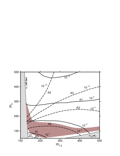
Figure 7: Contour plots in the $(m_{1/2},m_{0})$ plane for the decays $\mu\rightarrow e\gamma$ (left) and $\tau\rightarrow\mu\gamma$ (right), assuming $\tan\beta=10$ and $\mu<0$, and using the cases $A_{1}$(solid lines), $A_{3}$ (dashed). The rates for both decays are enhanced relative to the small $\tan\beta$ case. As a result, case $A_{3}$ is more favourable now in the dark-shaded region preferred by astrophysics and cosmology [48].

The light-shaded areas in Fig. 6 correspond to the regions of the $(m_{1/2},m_{0})$ plane that are excluded by LEP searches for charginos and by the requirement that the lightest supersymmetric particle not be charged [48]. The dark-shaded areas in Fig. 6 are those where the cosmological relic density is in the range preferred by astrophysics. We see that both the decay modes $\mu\rightarrow e\gamma$ and $\tau\rightarrow\mu\gamma$ could well be measurable throughout this astrophysical region. In particular, we find $BR(\tau\rightarrow\mu\gamma)>10^{-9}$ in most of this region, and for $m_{1/2}<220$ GeV and $m_{0}<110$ GeV there are regions where $BR(\tau\rightarrow\mu\gamma)>10^{-8}$. These observations also apply to texture B, and to the choice $\tan\beta=10$ (not shown). The predictions of texture C may also reach above $10^{-9}$, but reach above $10^{-8}$ only in a small portion of the cosmologically-favoured region. Texture B leads to the highest predictions for $BR(\mu\rightarrow e\gamma)$, typically above $10^{-12}$ for most of the cosmologically-favoured region of the $(m_{0},m_{1/2})$ plane, and even reaching values above $10^{-11}$ in a small portion of the parameter space. The sensitivity of the branching ratios to different choices of coefficients $c_{ij}$ can be seen by comparing the solid and dashed lines in Fig. 6. For $\tan\beta=3$, the obtained values for the branching ratios under consideration are smaller. A considerable sector of the cosmologically-favoured region, leads, however, to values for the branching ratios of the same order as the ones discussed above.

We show in Fig. 8 the correlation between the $\mu\rightarrow e\gamma$ and $\tau\rightarrow\mu\gamma$ branching ratios for two different choices of coefficients $c_{ij}$ for each of the textures A, B and C presented in Section 4. In each case, the branching ratios have been calculated for a sampling of $(m_{0},m_{1/2})$ pairs in the cosmologically-favoured region of [48] for $\tan\beta=10$: similar results hold for $\tan\beta=3$. We see clearly how the correlations between the two branching ratios vary with the choices of the $c_{ij}$ coefficients, because of their influences on flavor mixing. In the two cases $A_{1}$ and $A_{3}$ (texture $A_{2}$ is similar to $A_{1}$) presented in Fig. 8, the values of the predicted branching ratios are characteristic for each $c_{ij}$ set, with the case $A_{3}$ generally predicting smaller ratios for $BR(\mu\rightarrow e\gamma)/BR(\tau\rightarrow\mu\gamma)$. In the case of texture C, the dependence of the results on the choice of $c_{ij}$ coefficients is rather different: this texture tends to predict a relatively large ratio $BR(\mu\rightarrow e\gamma)/BR(\tau\rightarrow\mu\gamma)$.

Figure 8: Scatter plot of model predictions for $BR(\mu\rightarrow e\gamma)$ versus $BR(\tau\rightarrow\mu\gamma)$, assuming $tan\beta=10$ and $\mu<0$. The circles correspond to texture $A_{1}$, the + to texture $A_{2}$, the stars to texture $B_{1}$, the $\times$ to texture $B_{2}$ the squares to texture $C_{1}$, the diamonds to texture $C_{2}$. Note the characteristic correlations in the different models.

Finally, we show results for $\mu-e$ conversion, using both penguin and box diagrams. We gave in Section 2 an order-of-magnitude estimate of the branching ratio for this reaction, namely $BR(\mu Ti\rightarrow eTi)\approx 5.6\times 10^{-3}BR(\mu\rightarrow e\gamma)$. However, as we commented there, the two processes exhibit different functional dependences on the $A_{M/E}^{L,R}$ functions (indeed, as is well known, $\mu\rightarrow e\gamma$ does not depend at all on the parameters $A^{E}_{L,R}$). Further, in the case of $\mu-e$ conversion there are additional contributions from box graphs which further complicate the ratio $BR(\mu Ti\rightarrow eTi)/BR(\mu\rightarrow e\gamma)$. In view of the possible improvement of the experimental sensitivity to $\mu-e$ conversion, we present plots similar to given previously for $\mu\rightarrow e\gamma$.

It is instructive to compare the $\mu-e$ conversion rate with the corresponding predictions for $BR(\mu\rightarrow e\gamma)$, to explore the effects of penguin and box diagrams. In Fig.  9 we plot the ratio of the $\mu\rightarrow e$ conversion and $\mu\rightarrow e\gamma$ rates versus the scalar mass parameter $m_{0}$. We see immediately that the ratio is not constant, though its general order of magnitude is that estimated in (30). The dependence of the penguin contribution on $m_{0}$ is shown separately from the combined effects of penguin and box diagrams, for the two signs of $\mu$. In the case of $\mu>0$, $BR(\mu\rightarrow e\gamma)$ is relatively enhanced for large $m_{0}$ values, whilst the opposite is true for $\mu<0$.

Figure 9: The ratio of the $\mu\rightarrow e$ conversion rate to $BR(\mu\rightarrow e\gamma)$ is plotted versus $m_{0}$, for $\mu<0$. We plot the penguin contribution separately from the sum of the penguin and box diagrams, for $\tan\beta=3$ (left) and $\tan\beta=10$ (right).

We show in Fig. 10 the dependence of the $\mu\rightarrow e$ conversion rate on $m_{0}$ for the two textures $A,B$ and for the values $\tan\beta=3$ and $m_{1/2}=250$ GeV. As before, we choose three sets of numerical coefficients $c_{ij}$ for each texture, and exhibit the results for both signs of $\mu$. Interestingly, cases $A_{1},A_{2}$ give a rate close to the present experimental limit for most of the $m_{0}$ region explored when $\mu>0$. The corresponding predictions for $\mu<0$ are considerably lower for large $m_{0}$ values, but converge with those of the $\mu>0$ case for small $m_{0}$. We note that texture B exhibits greater sensitivity to the coefficients $c_{ij}$ than does texture A.

Figure 10: The muon conversion rate $\mu\rightarrow e$ as a function of $m_{0}$ for the textures A and B, assuming $\tan\beta=3$. The solid lines correspond to $\mu>0$ and the dashed to $\mu<0$.

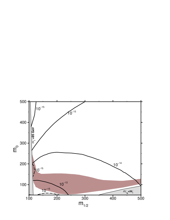
Figure 11: Contour plots in the $(m_{1/2},m_{0})$ plane for $\mu\rightarrow e$ conversion, assuming $\tan\beta=3$ and $\mu<0$ and using the cases $A_{1},A_{3}$. We see that the conversion rate is encouraging throughout the dark-shaded region preferred by astrophysics and cosmology [48] in the scenario $A_{1}$.

Fig. 11 displays contours of the rate for $\mu\rightarrow e$ conversion in the $(m_{0},m_{1/2})$ plane for the two scenarios $A_{1}$ and $A_{3}$. We see that the former predicts a rather larger rate, which offers good prospects for observation throughout the region preferred by cosmology. On the other hand, scenario $A_{3}$ predicts a rather lower rate for $\mu\rightarrow e$ conversion.

We comment at this stage on some of the ambiguities in the results shown above, within the general $U(1)$ framework studied. We have already explored to some extent the ambiguity associated with ${\cal O}(1)$ coefficients in the Dirac mass matrices for the fermions. The ambiguity induced by simple sign changes can be particularly acute, as we illustrate with one simple exercise. For example, since the light Majorana mixing matrix is $V_{MNS}=V_{\ell}V_{\nu}^{\dagger}$, any modification that changes the relative signs of off-diagonal entries in $V_{\ell}$ and $V_{\nu}$ could cause large changes in the mixing angles of $V_{MNS}$, as one changes from destructive to constructive interference, or vice versa, with intermediate possibilities corresponding to various phase possibilities that are not specified by the $U(1)$ symmetry.

As an exercise, using the numerical values of the coefficients in the case $A_{1}$ discussed above, we invert the signs of all the off-diagonal entries in $m_{\nu}^{D}$, and repeat consistently all the subsequent steps in the calculations. The implications for $\mu\rightarrow e\gamma$ and $\tau\rightarrow\mu\gamma$ are shown in Fig. 12, where we see that $BR(\mu\rightarrow e\gamma)$ may be increased by about two orders of magnitude , whereas that for $BR(\tau\rightarrow\mu\gamma)$ is increased by less than an order of magnitude. This ‘inverted’ $U(1)$ model actually has much larger $\nu_{\mu}-\nu_{\tau}$ mixing than the ‘uninverted’ version of $A_{1}$, or indeed the other textures studied previously, agreeing better with the Super-Kamiokande data. We interpret the difference between $A_{1}$ and ‘inverted’ $A_{1}$, on the one side, and between $A_{1}$ and $A_{3}$, on the other side, as indicative of the numerical ambiguity within any particular texture . We see that the predictions for $\mu\rightarrow e\gamma$ are very variable, bracketing the present experimental upper limit within a broad range, whereas the predictions for $\tau\rightarrow\mu\gamma$ are more closely bunched, and likely to be within reach of experiment.

Figure 12: Predictions of $BR(\mu\rightarrow e\gamma)$ and $BR(\tau\rightarrow\mu\gamma)$ in the ‘inverted’ version of $A_{1}$, obtained by inverting the signs of all the off-diagonal terms in $m_{\nu}^{D}$, for $\mu<0$.

The generality of these features is left for exploration in the future. There are also other ambiguities, for example in the choice of the heavy Majorana mass matrix [47], whose detailed study we also leave for future work.

Before concluding, we make a few more remarks about non-Abelian models, and about the flipped $SU(5)$ model. As commented at the end of subsection IV-B, generic non-Abelian models would fall into our ‘mismatched’ category, and we would expect them to have relatively large rates for both $\mu\rightarrow e$ and $\tau\rightarrow\mu$ transitions, as a result of their preference for near-bi-maximal mixing. Therefore, we expect the prospects for charged-lepton-flavour violation in these models to be at least as favourable as in the Abelian models studied here. In the case of flipped $SU(5)$, if we use naively the matrices displayed in Section 5, we find that the $\mu\rightarrow e\gamma$ process is rather enhanced, and it exceeds the present experimental bounds in a considerable region of the parameter space, at least for some generic choices of undetermined numerical coefficients. However, since the plethora of poorly-constrained expansion parameters introduces ambiguities, as discussed earlier, a complete exploration of this model is beyond the scope of this paper, and it may be that the model can survive for suitable values of these coefficients. On the other hand, the $\tau\rightarrow\mu\gamma$ reaction is highly suppressed, because in this model all the mixing needed to interpret the atmospheric neutrino data comes from the neutrino sector, and there is no mixing in the $\tau-\mu$ charged-lepton sector.

6. Conclusions

Although family symmetries provide many interesting insights into the hierarchy of fermion masses, there is no unique framework that fits the available information on charged fermions and neutrinos. As a result, there is considerable ambiguity, even within the subclass of Abelian flavour models, in their predictions for charged-lepton-flavour violation. We have explored some of the range of possibilities in this paper. Many sets of undetermined ${\cal O}(1)$ coefficients in Abelian flavour symmetry models of the charged lepton mass matrix can fit well the mass spectrum and the neutrino data, but vary in their predictions for the branching ratios of rare processes. As examples, three different sets of coefficients were used to fit the charged lepton and quark mass matrices in each of three Abelian texture models. Our studies show that these vary in their predictions for flavour-changing branching ratios by up to two orders of magnitude. The good news, however, is that many of these models seem to be accessible to a new round of experiments searching for $\mu\rightarrow e$ and $\tau\rightarrow\mu$ transitions. In particular, we would like to re-emphasize the interest of exploring the branching ratio for $\tau\rightarrow\mu\gamma$ down to the $10^{-9}$ level or below, as may be possible at the LHC.

In view of their accessibility, and precisely because of their model-dependence, such rare decays may become a powerful tool for distinguishing between different neutrino textures. As we have seen, textures based on Abelian flavour symmetries tend to predict relatively small $\mu-e$ flavour mixing, thus leading to rates for $\mu\rightarrow e\gamma$, $\mu\rightarrow 3e$ and $\mu\to e$ conversion in nuclei that are generically below the experimental bounds, though close enough to offer interesting physics opportunities for experiments with present and future intense $\mu$ sources. On the other hand, schemes based on non-Abelian flavour symmetries would tend to predict large mixing in the (1-2) lepton sector. In this case, larger rates are likely to be found for the above processes, and in certain textures part of the supersymmetric parameter space may already be excluded. It is likely also that string-derived flipped $SU(5)$ schemes based on would have large off-diagonal entries in the (1-2) lepton sector, leading to larger rates for $\mu\rightarrow e\gamma$, $\mu\rightarrow 3e$ and $\mu\to e$ conversion in nuclei than the simplest models with Abelian flavour symmetries, though the rates for $\tau\rightarrow\mu\gamma$ would be relatively low.

We conclude by encouraging the community to pursue actively new generations of experiments to probe charged-lepton-flavour violation, in both $\mu$ and $\tau$ decays. Such efforts would complement nicely the physics being revealed by neutrino oscillations, and could provide precious insight into the flavour problem.

Acknowledgements
M.E.G. thanks D. Carvalho for useful discussions, and his research has been supported by the European Union TMR Network contract ERBFMRX-CT96-0090.

Note Added
While this paper was in the final stages of preparation, we received the paper by Feng, Nir and Shadmi in [9], which makes points similar to ours, in a complimentary way.

References

- [1] Y. Fukuda et al., Super-Kamiokande collaboration, Phys. Lett. B433 (1998) 9; Phys. Lett. B436 (1998) 33; Phys. Rev. Lett. 81 (1998) 1562.
- [2] M. Apollonio et al., Chooz collaboration, Phys. Lett. B420 (1998) 397.
- [3] See for example, L. Wolfenstein, Phys. Rev. D17 (1978) 20; S. P. Mikheyev and A.Yu. Smirnov, Yad. Fiz. 42 (1985) 1441 and Sov. J. Nucl. Phys. 42 (1986) 913.
- [4] S.T. Petcov Yad. Phys. 25 (1977) 641 and Sov. J. Nucl. Phys. 25 (1977) 340; S.M. Bilenki, S.T. Petcov and B. Pontecorvo, Phys. Lett. B67 (1977) 309.
- [5] F. Borzumati and A. Masiero, Phys. Rev. Lett. 57 (1986) 961; G.K. Leontaris, K. Tamvakis and J.D. Vergados, Phys. Lett. B171 (1986) 412; T.S. Kosmas et al., Phys. Lett. B219 (1989) 457; J. Hisano, T. Moroi, K. Tobe and M. Yamaguchi, Phys. Lett. B357 (1995) 579; Phys. Lett. B391 (1997) 341, [Erratum - ibid. B397 (1997) 357] and Phys. Rev. D53 (1996) 2442; S.F. King and M. Oliveira, Phys. Rev. D60 (1999) 035003.
- [6] J. Ellis and D.V. Nanopoulos, Phys. Lett. B110 (1982) 44; R. Barbieri and R. Gatto, Phys. Lett. B110 (1982) 211; L.J. Hall, V.A. Kostelecky and S. Raby, Nucl. Phys. B267 (1986) 415; F. Gabianni and A. Masiero, Nucl. Phys. B322 (1989) 235; A. E. Faraggi, J.L. Lopez, D.V. Nanopoulos and K. Yuan Phys. Lett. B221 (1989) 337; S. Kelley, J.L. Lopez, D.V. Nanopoulos and H. Pois, Nucl. Phys. B358 (1991) 27.
- [7] R. Barbieri and L.J. Hall, Phys. Lett. B338 (1994) 212; R. Barbieri et al., Nucl. Phys. B445 (1995) 219; S. Dimopoulos and D. Sutter, Nucl. Phys. B452 (1995) 496; Nima Arkani-Hamed, Hsin-Chia Cheng and L.J. Hall, Phys. Rev. D 53 (1996)413-436; P. Ciafaloni, A. Romanino and A. Strumia, Nucl. Phys. B458 (1996) 3; M.E. Gómez and H. Goldberg, Phys. Rev. D53 (1996) 5244 ; Nucl. Phys. Proc. Suppl. 52A (1997) 163; B. de Carlos, J.A. Casas and J.M. Moreno, Phys.Rev. D53 (1996) 6398; A. Ilakovac and A. Pilaftsis, Nucl. Phys. B 437 (1995) 491; G.K. Leontaris and N.D. Tracas, Phys. Lett. B419 (1998) 206 and Phys. Lett. B431 (1998) 90; W. Buchmuller, D. Delepine and F. Vissani, Phys. Lett. B459 (1999) 171; J. Hisano and D. Nomura, Phys. Rev. D59 (1999) 116005; C.S. Lim and B. Taga, hep-ph/9812314; K. Kurosawa and N. Maekawa, Prog. Theor. Phys. 102 (1999) 121; R. Kitano and K. Yamamoto, hep-ph/9905459; Y. Okada and K. Okumura, hep-ph/9906446.
- [8] M. Gómez, G. Leontaris, S. Lola and J. Vergados, Phys. Rev. D59 (1999) 116009.
- [9] J.L. Feng, Y. Nir and Y. Shadmi, hep-ph/9911370.
- [10] For a recent review, see: Y. Kuno and Y. Okada, hep-ph/9909265.
- [11] M.L. Brooks et al., MEGA collaboration, hep-ex/9905013.
- [12] U. Bellgardt et al., Nucl. Phys. B229 (1988) 1.
- [13] P. Wintz, Proceedings of the First International Symposium on Lepton and Baryon Number Violation, eds. H.V. Klapdor-Kleingrothaus and I.V. Krivosheina (Institute of Physics, Bristol, 1998), p.534.
- [14] S. Ahmed et al., CLEO Collaboration, hep-ex/9910060.
- [15] L.M. Barkov et al., Research Proposal for an experiment at PSI (1999).
- [16] SINDRUM II collaboration, Research Proposal for an experiment at PSI (1999).
- [17] M. Bachmann et al., MECO collaboration, Research Proposal E940 for an experiment at BNL (1997).
- [18] L. Serin and R. Stroynowski, ATLAS Internal Note (1997) report a possible sensitivity to , which may be improvable, perhaps to the level of , private communications from D. Denegri and F. Gianotti.
- [19] See, for example: Workshop on Physics at the first Muon Collider and at the Front End of the Muon Collider, eds. S. Geer and R. Raja, AIP Conf. Proc. 435 (1998), particularly the contribution by W.J. Marciano; Prospective Study of Muon Storage Rings at CERN, eds. B. Autin, A. Blondel and J. Ellis, CERN Report 99-02 (1999).
- [20] M. Gell-Mann, P. Ramond and R. Slansky, proceedings of the Stony Brook Supergravity Workshop, New York, 1979, eds. P. Van Nieuwenhuizen and D. Freedman (North-Holland, Amsterdam).
- [21] J. Ellis, C. Kounnas and D.V. Nanopoulos, Nucl. Phys. B247 (1984) 373; J. Ellis, A.B. Lahanas, D.V. Nanopoulos and K. Tamvakis, Phys. Lett. B134 (1984) 429.
- [22] M. Dine and A. Nelson, Phys. Rev. D48 (1993) 1277; M. Dine, A. Nelson and Y. Shirman, Phys. Rev. D51 (1995) 1362; M. Dine, A. Nelson, Y. Nir and Y. Shirman, Phys. Rev. D53 (1996) 2658; S. Dimopoulos, S. Thomas and J.D. Wells, Nucl. Phys. B488 (1997) 39; G. Giudice and R. Rattazzi, hep-ph/9801271, and references therein.
- [23] See for instance some of the textures studied by G. Altarelli and F. Feruglio, Phys. Lett. B439 (1998) 112 and JHEP 9811 (1998) 021.
- [24] J. Ellis, G.K. Leontaris, S. Lola and D.V. Nanopoulos, Eur. Phys. J. C9 (1999) 389.
- [25] G.K. Leontaris, S. Lola and G.G. Ross, Nucl. Phys. B454 (1995) 25.
- [26] S. Lola and G.G. Ross, Nucl. Phys. B553 (1999) 81.
- [27] V. Barger, S. Pakvasa, T.J. Weiler and K. Whisnant, Phys. Lett. B437 (1998) 107; A.J. Baltz, A.S. Goldhaber and M. Goldhaber, Phys. Rev. Lett. 81 (1998) 5730. See also: R. N. Mohapatra and S. Nussinov, Phys. Lett. B441 (1998) 299 and hep-ph/9809415; C. Jarlskog, M. Matsuda and S. Skadhauge, hep-ph/9812282; Y. Nomura and T. Yanagida, Phys. Rev. D59 (1999) 017303; S.K. Kang and C.S. Kim, Phys. Rev. D59 (1999) 091302; H. Georgi and S.L. Glashow, hep-ph/9808293.
- [28] Some of the many references are: C. Wetterich, Nucl. Phys. B261 (1985) 461; G.K. Leontaris and D.V. Nanopoulos, Phys. Lett. B212 (1988) 327; Y.Achiman and T. Greiner, Phys. Lett. B329 (1994) 33; H. Dreiner et al., Nucl. Phys. B436 (1995) 461. Y. Grossman and Y. Nir, Nucl. Phys. B448 (1995) 30; P. Binétruy, S. Lavignac and P. Ramond, Nucl. Phys. B477 (1996) 353; G.K. Leontaris, S. Lola, C. Scheich and J.D. Vergados, Phys. Rev. D 53 (1996) 6381; S. Lola and J.D. Vergados, Progr. Part. Nucl. Phys. 40 (1998) 71; B.C. Allanach, hep-ph/9806294; P. Binétruy et al., Nucl. Phys. B496 (1997) 3, G. Altarelli and F. Feruglio, Phys. Lett. B451 (1999) 388 and hep-ph/9905536; G. Altarelli, F. Feruglio and I. Masina, hep-ph/9907532; Y. Nir and Y. Shadmi, JHEP 9905 (1999) 023.
- [29] Y. L. Wu, Phys. Rev. D59 (1999) 113008; Eur. Phys. J. C10 (1999) 491; Int. J. Mod. Phys. A14 (1999) 4313; C. Wetterich, Phys. Lett. B451 (1999) 397; R. Barbieri, L. J. Hall, G. L. Kane, and G. G. Ross, hep-ph/9901228.
- [30] I. Antoniadis, J. Ellis, J. Hagelin and D.V. Nanopoulos, Phys. Lett. B194 (1987) 231; Phys. Lett. B231 (1989) 65.
- [31] See for instance the last two papers in [5] and references therein.
- [32] S. Weinberg and G. Feinberg, Phys. Rev. Lett. 3 (1959) 111.
- [33] N. Cabibbo and R. Gatto, Phys. Rev. 116 (1959) 1334.
- [34] H. Primakoff and P.S. Rosen, Ann. Rev. Nucl. Part. Sci. 31 (1981) 145.
- [35] T.S. Kosmas, A. Faessler and J.D. Vergados, J. Phys. G G23 (1997) 693.
- [36] T.S. Kosmas, A. Faessler, F. Simkovic and J.D. Vergados, Phys. Rev. C56 (1997) 526.
- [37] Z. Maki, M. Nakagawa and S. Sakata, Prog. Theor. Phys. 28 (1962) 247.
- [38] M. Carena, J. Ellis, S. Lola and C.E.M. Wagner, hep-ph/9906362, to appear in the Eur. Phys. J. C.
- [39] J. Ellis and S. Lola, Phys. Lett. B458 (1999) 310.
- [40] A. Casas, J.R. Espinosa, A. Ibarra and I. Navarro, Nucl. Phys. B556 (1999) 3; JHEP 9909 (1999) 015; hep-ph/9905381; hep-ph/991042; N. Haba, Y. Matsui, N. Okamura and M. Sigiura, Eur. Phys. J. C10 (1999) 677 and hep-ph/9908429; N. Haba, N. Okamura and M. Sigiura, hep-ph/9810471; N. Haba and N. Okamura, hep-ph/9906481.
- [41] C. D. Froggatt and H. B. Nielsen, Nucl. Phys. B147 (1979) 277.
- [42] L. Ibanez and G.G. Ross, Phys. Lett. B332 (1994) 100.
- [43] S. Lola, hep-ph/9903203, to appear in Proceedings of the 1998 Corfu Summer Institute on Elementary Particle Physics, to be published in JHEP.
- [44] M. Schmaltz, Phys. Rev. D52 (1995) 1643; H. Fritzsch and Z. Xing, Phys. Lett. B372 (1996) 265 and Phys. Lett. B440 (1998) 313; K. Kang, S.K. Kang, J.E. Kim and P. Ko, Mod. Phys. Lett. A12, (1997) 1175; M. Fukugita, M. Tanimoto and T. Yanagida, Phys. Rev. D57 (1998) 4429; P.H. Frampton and A. Rasin, hep-ph/9910522; R. Dermisek and S. Raby, hep-ph/991127.
- [45] R. Barbieri, G.G. Ross and A. Strumia, JHEP 9910 (1999) 020.
- [46] S. Kalara, J.L. Lopez and D.V. Nanopoulos, Nucl. Phys. B353 (1991) 650; S. Kalara, J.L. Lopez and D.V. Nanopoulos, Phys. Lett. B245 (1990) 421; J. Rizos and K. Tamvakis, Phys. Lett. B262 (1991) 227.
- [47] J. Ellis, G.K. Leontaris, S. Lola and D.V. Nanopoulos, Phys. Lett. B425 (1998) 86.
- [48] J. Ellis, T. Falk and K. A. Olive, Phys. Lett. B444 (1998) 367; J. Ellis, T. Falk, K. A. Olive and M. Srednicki, hep-ph/9905481; A.B. Lahanas, D.V. Nanopoulos and V.C. Spanos, hep-ph/9909497.