DESY 99–174
TTP99–47
hep-ph/9911434
November 1999

The relation between the $\overline{\rm MS}$ and the on-shell quark mass at order $\alpha_{s}^{3}$

Abstract

The relation between the on-shell and $\overline{\rm MS}$ mass can be expressed through scalar and vector part of the quark propagator. In principle these two-point functions have to be evaluated on-shell which is a non-trivial task at three-loop order. Instead, we evaluate the quark self energy in the limit of large and small external momentum and use conformal mapping in combination with Padé improvement in order to construct a numerical approximation for the relation [2]. The errors of our final result are conservatively estimated to be below 3%. The numerical implications of the results are discussed in particular in view of top and bottom quark production near threshold. We show that the knowledge of new ${\cal O}(\alpha_{s}^{3})$ correction leads to a significant reduction of the theoretical uncertainty in the determination of the quark masses.

1 Introduction

In higher order calculations there is in general an ambiguity in the prediction for the physical quantities which can be traced back to the adopted renormalization scheme. Different renormalization conditions imply different numerical values for the parameters of the underlying theory. Very often it is useful to convert them from one scheme into an other in order to compare the final predictions for the observables in both schemes.

In Quantum Chromodynamics (QCD) practical calculations are very often performed in the modified minimal subtraction ($\overline{\rm MS}$) scheme [3, 4] leading to the definition of the so-called short-distance $\overline{\rm MS}$ mass. The $\overline{\rm MS}$ mass occupies a distinguished place among various mass definitions. First, it is a truly short distance mass not suffering from nonperturbative ambiguities. Second, the $\overline{\rm MS}$ mass proves to be extremely convenient in multi-loop calculations of mass-dependent inclusive physical observables dominated by short distances (for a review see [5]). On the other hand the experiments often provide masses which are tightly connected to the on-shell definition. Thus, conversion formulae are needed in order to make contact between theory and experiment. The two-loop relation between $\overline{\rm MS}$ and the on-shell definition of the quark mass has been obtained in [6] and has been confirmed in [7]. Until recently the accuracy of this equation was enough for the practical applications. Meanwhile, however, new computations have become available which require the relation between the $\overline{\rm MS}$ and on-shell mass at ${\cal O}(\alpha_{s}^{3})$ in order to perform a consistent analysis. The necessity of an accurate determination of the quark masses, especially those of the top and bottom ones, is demonstrated by the following two examples.

The main goal of the future $B$ physics experiments is the determination of the Cabibbo-Kobayashi-Maskawa matrix elements which will give deeper insight into the origin of CP violation and possibly also provides hints to new physics. In particular the precise measurement of $V_{cb}$ is very promising. It is determined from semileptonic $B$ meson decay rates. Thus it is desirable to know the bottom quark mass as accurately as possible as it enters already the Born result to the fifth power.

One of the primary goals of a future electron-positron linear collider or muon collider will be the precise determination of the top quark properties, especially its mass, $M_{t}$. In hadron colliders like the Fermilab TEVATRON or the Large Hadron Collider the top quarks are reconstructed from the invariant mass of the $W$ bosons and the bottom quarks. On the contrary in lepton colliders it is possible to determine the top quark mass from the line shape of the production cross section $\sigma(e^{+}e^{-}\to t\bar{t})$ close to the threshold. Simulation studies have shown that an experimental uncertainty of about $100$ MeV in the top mass determination can be achieved [8]. Thus also from the theoretical side the ambiguities have to be controlled with the same precision.

Threshold phenomena are conveniently expressed in terms of the pole mass, $M$, of the corresponding quark as this parameter naturally appears in the equations which have to be solved. The pole mass is a gauge invariant, infrared-finite and a renormalization scheme independent quantity [9, 10, 11, 12]. However, various calculations [13] have shown that higher order corrections have an significant influence on the predictions for the quark production cross section. It has been shown that this is connected to the definition of the quark mass used for the parameterization of the cross section [14, 15]. A common remedy is the introduction of a new mass parameter which is supposed to be insensitive to long distance phenomena. One thus often speaks about short-distance masses. The relation of the new mass parameter to the pole mass is used in order to re-parameterize the threshold phenomena. On the other hand a relation of the new quark mass to the $\overline{\rm MS}$ mass must be established as it is commonly used for the parameterization of those quantities which are not related to the threshold.

Recently several groups evaluated next-to-next-to-leading order results for the cross section $\sigma(e^{+}e^{-}\to t\bar{t})$ close to threshold [13, 16, 17, 18, 19]. In order to establish a consistent relation to the $\overline{\rm MS}$ mass the three-loop relation between the $\overline{\rm MS}$ and the on-shell mass is needed. This will be discussed in Section 7.

The bottom quark mass can be obtained from sum rules for the $\Upsilon$ mesons [20, 21]. The current strategy can be schematically outlined as follows [22, 23, 24]. Moments of the current correlator involving bottom quarks are determined with the help of experimental results on the electronic decay width and the masses of the $\Upsilon$ mesons. They are compared with the moments computed with the help of non-relativistic QCD. Due to the strong dependence on the bottom quark mass a precise determination is possible. Recently a next-to-next-to-leading order computation has become available [25, 26]. Again, for a consistent determination of the $\overline{\rm MS}$ mass the order $\alpha_{s}^{3}$ relation to the on-shell mass is necessary.

A somewhat different approach for the determination of both the charm and bottom mass has been performed in [27]. The lower states in the heavy quarkonium spectrum have been computed up to order $\alpha_{s}^{4}$ which again demands for the three-loop $\overline{\rm MS}$–on-shell mass relation in order to evaluate the $\overline{\rm MS}$ mass.

Another application where the three-loop relation between the on-shell and the $\overline{\rm MS}$ mass is needed is connected the recent evaluation of the quartic mass corrections at order $\alpha_{s}^{3}$ to the cross section $\sigma(e^{+}e^{-}\to\mbox{hadrons})$ [28, 29]. For conceptual reasons the calculation has been performed using the $\overline{\rm MS}$ mass. If, however, the result should be expressed in terms of the pole mass the corresponding relation has to be known to order $\alpha_{s}^{3}$. Note the Born result expanded for small quark masses doesn’t have a quadratic term. Thus in this case the mass relation is only needed up to order $\alpha_{s}^{2}$ and the quartic corrections require for the first time the ${\cal O}(\alpha_{s}^{3})$ terms.

In the present article we describe the calculation of the ${\cal O}(\alpha_{s}^{3})$ correction to the mass relation as well as the implications of the result. A short version containing the main results has been published in [2].

The outline of the paper is as follows. In the next section the notation is introduced. Afterwards in Section 3 the method we use for the calculation is described in detail. Its power is demonstrated in Section 4 at the one- and two-loop level where a comparison with the exact results is possible. The tools needed for the three-loop calculation are presented in Section 5. In particular we collect all difficult integrals which are needed for the computation of the fermion propagator. The three-loop results for the mass relation are finally discussed in Section 6 and their implications to quark production processes are mentioned in Section 7. Our conclusions are presented in Section 8.

2 Notation

This section is devoted to set up the notation. Throughout this paper the bare (unrenormalized) mass is denoted by $m^{0}$ and the $\overline{\rm MS}$ and on-shell renormalized ones by $m$ and $M$, respectively. Their connection is given by the following equations

$$m(\mu) = Z_{m}m^{0}\,\,=\,\,z_{m}(\mu)M\,,$$ (1)

where $z_{m}$ is finite and has an explicit dependence on the renormalization scale $\mu$. The main goal of this paper is the computation of $z_{m}$ up to order $\alpha_{s}^{3}$. Therefore three-loop corrections to the fermion propagator have to be considered. A convenient variable in this context is

$$z = \frac{q^{2}}{M^{2}}\,,$$ (2)

where $q$ is the external momentum of the fermion propagator.

The inverse quark propagator is denoted by

$$\left(S_{F}^{0}(q)\right)^{-1} = i\left[m^{0}\left(1-\Sigma_{S}^{0}\right)-q\left(1+\Sigma_{V}^{0}\right)\right]\,,$$ (3)

where the functions $\Sigma_{S}^{0}$ and $\Sigma_{V}^{0}$ depend on the external momentum $q$, the bare mass $m^{0}$ and on the bare strong coupling constant $\alpha_{s}^{0}$. The renormalized version can be cast in the form

$$\left(S_{F}(q)\right)^{-1} = i\left[\left(M-q\right)S_{V}(z)+M\left(z_{m}(\mu)S_{S}(z)-S_{V}(z)\right)\right]\,,$$ (4)

with

$$S_{V}(z) = Z_{2}(1+\Sigma^{0}_{V})\,,$$

$$S_{S}(z) = Z_{2}Z_{m}(1-\Sigma^{0}_{S})\,.$$ (5)

$Z_{2}$ denotes the wave function renormalization in the $\overline{\rm MS}$ scheme which is sufficient for our considerations. Note that the functions $S_{S}$ and $S_{V}$ are $\overline{\rm MS}$ quantities which later on are expressed in terms of the on-shell mass. The two-loop relation between $m$ and $M$ is enough to do this at order $\alpha_{s}^{3}$.

It is convenient to write the functions $S_{S/V}$ in the following way:

$$S_{S/V}=1+\sum_{n\geq 1}S_{S/V}^{(n)}\left(\frac{\alpha_{s}}{\pi}\right)^{n}\,,$$ (6)

where the quantities $S_{S/V}^{(n)}$ exhibit the following colour structures (the indices $S$ and $V$ are omitted in the following):

$$S^{(1)} = C_{F}S_{F}\,,$$

$$S^{(2)} = C_{F}^{2}S_{FF}+C_{F}C_{A}S_{FA}+C_{F}Tn_{l}S_{FL}+C_{F}TS_{FH}\,,$$

$$S^{(3)} = C_{F}^{3}S_{FFF}+C_{F}^{2}C_{A}S_{FFA}+C_{F}C_{A}^{2}S_{FAA}+C_{F}^{2}Tn_{l}S_{FFL}+C_{F}^{2}TS_{FFH}$$ (7)

$$\mbox{}+C_{F}C_{A}Tn_{l}S_{FAL}+C_{F}C_{A}TS_{FAH}+C_{F}T^{2}n_{l}^{2}S_{FLL}+C_{F}T^{2}n_{l}S_{FLH}$$

$$\mbox{}+C_{F}T^{2}S_{FHH}\,.$$

The same decomposition also holds for the function $z_{m}$. In (7) $n_{l}$ represents the number of light (massless) quark flavours. $C_{F}$ and $C_{A}$ are the Casimir operators of the fundamental and adjoint representation. In the case of $SU(N_{c})$ they are given by $C_{F}=(N_{c}^{2}-1)/(2N_{c})$ and $C_{A}=N_{c}$. The trace normalization of the fundamental representation is $T=1/2$. The subscripts $F$, $A$ and $L$ in Eq. (7) shall remind on the colour factors $C_{F}$, $C_{A}$ and $Tn_{l}$, respectively. $H$ simply stands for the colour factor $T$.

At one- and two-loop order the results for $z_{m}$ read [9, 6]

$$z_{m}^{F}(\mu) = -1-\frac{3}{4}l_{\mu M}\,,$$

$$z_{m}^{FF}(\mu) = \frac{7}{128}-\frac{15}{8}\zeta_{2}-\frac{3}{4}\zeta_{3}+3\zeta_{2}\ln 2+\frac{21}{32}\,l_{\mu M}+\frac{9}{32}\,l_{\mu M}^{2}\,\,\approx\,\,-0.51056\,,$$

$$z_{m}^{FA}(\mu) = -\frac{1111}{384}+\frac{1}{2}\zeta_{2}+\frac{3}{8}\zeta_{3}-\frac{3}{2}\zeta_{2}\ln 2-\frac{185}{96}\,l_{\mu M}-\frac{11}{32}\,l_{\mu M}^{2}\,\,\approx\,\,-3.33026\,,$$

$$z_{m}^{FL}(\mu) = \frac{71}{96}+\frac{1}{2}\zeta_{2}+\frac{13}{24}\,l_{\mu M}+\frac{1}{8}\,l_{\mu M}^{2}\,\,\approx\,\,1.56205\,,$$

$$z_{m}^{FH}(\mu) = \frac{143}{96}-\zeta_{2}+\frac{13}{24}\,l_{\mu M}+\frac{1}{8}\,l_{\mu M}^{2}\,\,\approx\,\,-0.15535\,,$$ (8)

with $l_{\mu M}=\ln\mu^{2}/M^{2}$ where after the approximation signs the choice $\mu^{2}=M^{2}$ has been adopted. For later use we also define the propagator of the gluon. In ’t Hooft-Feynman gauge it is given by

$$D_{g}(q) = i\frac{-g^{\mu\nu}+\xi\frac{q^{\mu}q^{\nu}}{q^{2}}}{q^{2}+i\epsilon}\,.$$ (9)

3 Method

A formula which allows for the computation of the $\overline{\rm MS}$–on-shell relation for the quark mass is obtained from the requirement that the inverse fermion propagator has a zero at the position of the on-shell mass:

$$\left(S_{F}(q)\right)^{-1}\bigg{|}_{q^{2}=M^{2}} = 0\,.$$ (10)

At order $\alpha_{s}^{3}$ this requires the evaluation of three-loop on-shell integrals. Currently it is quite unhandy to deal with such kind of diagrams as up to now the literature lacks of a useful description of an algorithm for their computation. Even though the technology is in principle available as it was needed for the computation of the anomalous magnetic moment of the muon [31].

We have decided to choose a different way for the practical calculation. The starting point is, of course, also Eq. (10). Applying it to Eq. (4) leads to the condition

$$f(z) \equiv z_{m}(\mu)\,S_{S}(z)-S_{V}(z)\,\,=\,\,0\qquad\mbox{for}\qquad z=1\,.$$ (11)

At a given loop-order $L$ the Eqs. (5) are inserted and the resulting equation is solved for $z_{m}^{(L)}$. Thus Eq. (11) can be cast in the form

$$f(z) = g(z)+z_{m}^{(L)}\left(\frac{\alpha_{s}}{\pi}\right)^{L}\,.$$ (12)

Our aim is the computation of $g(1)$. Note that the individual self energies $\Sigma_{S}$ and $\Sigma_{V}$ develop infra-red singularities when they are evaluated on-shell. The proper combination which leads to the relation between the $\overline{\rm MS}$ and on-shell mass is, however, free of infra-red problems.

At this point a comment in connection to Eq. (11) is in order. In fact also more involved equations could be chosen which result in more complicated expressions for $g(z)$. To us the choice in (11) appears very natural. Furthermore the one- and two-loop results are reproduced with rather high accuracy. We also tried various other options; the final results, however, remained the same.

The strategy for the computation of $g(1)$ is as follows [32]: Expansions for small and large external momentum are computed for the quark self energies. After building the proper combinations needed for $g(z)$ a conformal mapping [33] is performed

$$z = \frac{4\omega}{(1+\omega)^{2}}\,,$$ (13)

which maps the complex $z$-plane into the interior of the unit circle in the $\omega$-plane. The relevant point $z=1$ is mapped to $\omega=1$. The motivation for this conformal mapping is based on the observation that the application of a Padé approximation relies heavily on analytic properties. Actually, $g(z)$ develops a branch cut along the real $z$-axis starting from $z=1$. This cut is mapped through Eq. (13) onto the unit circle of the $\omega$ plane. Thus by applying Eq. (13) the radius of convergence is enlarged. In order to ensure also the convergence at the boundary a Padé approximation is performed. In the variable $\omega$ it is defined through

$$[m/n](\omega) = \frac{a_{0}+a_{1}\omega+\ldots+a_{m}\omega^{m}}{1+b_{1}\omega+\ldots+b_{n}\omega^{n}}\,.$$ (14)

The details for the construction of the Padé approximants can be found in [34]. Special care has to be taken with the logarithms $\ln(-q^{2})$ which occur in the results of the high-energy expansions as they could destroy the convergence properties of the described procedure. Details on their treatment can be found in [34, 35].

The described procedure is applied to each colour structure occurring in $g(z)$ separately. If we assume that the decomposition introduced in Eqs. (6) and (7) also holds for $g(z)$ the following equations are obtained

$$g_{F}(z)\,\,=\,\,S_{S,F}(z)-S_{V,F}(z)\,,\qquad\qquad\quad\,\,g_{FA}(z)\,\,=\,\,S_{S,FA}(z)-S_{V,FA}(z)\,,$$

$$g_{FL}(z)\,\,=\,\,S_{S,FL}(z)-S_{V,FL}(z)\,,\qquad\qquad g_{FH}(z)\,\,=\,\,S_{S,FH}(z)-S_{V,FH}(z)\,,$$

$$g_{FF}(z)\,\,=\,\,S_{S,FF}(z)-S_{V,FF}(z)+z_{m}^{F}S_{S,F}\,,$$

$$g_{FAA}(z)\,\,=\,\,S_{S,FAA}(z)-S_{V,FAA}(z)\,,\qquad\,\,g_{FAL}(z)\,\,=\,\,S_{S,FAL}(z)-S_{V,FAL}(z)\,,$$

$$g_{FAH}(z)\,\,=\,\,S_{S,FAH}(z)-S_{V,FAH}(z)\,,\qquad g_{FLL}(z)\,\,=\,\,S_{S,FLL}(z)-S_{V,FLL}(z)\,,$$

$$g_{FLH}(z)\,\,=\,\,S_{S,FLH}(z)-S_{V,FLH}(z)\,,\qquad g_{FHH}(z)\,\,=\,\,S_{S,FHH}(z)-S_{V,FHH}(z)\,,$$

$$g_{FFF}(z)\,\,=\,\,S_{S,FFF}(z)-S_{V,FFF}(z)+z_{m}^{F}S_{S,FF}+z_{m}^{FF}S_{S,F}\,,$$

$$g_{FFA}(z)\,\,=\,\,S_{S,FFA}(z)-S_{V,FFA}(z)+z_{m}^{F}S_{S,FA}+z_{m}^{FA}S_{S,F}\,,$$

$$g_{FFL}(z)\,\,=\,\,S_{S,FFL}(z)-S_{V,FFL}(z)+z_{m}^{F}S_{S,FL}+z_{m}^{FL}S_{S,F}\,,$$

$$g_{FFH}(z)\,\,=\,\,S_{S,FFH}(z)-S_{V,FFH}(z)+z_{m}^{F}S_{S,FH}+z_{m}^{FH}S_{S,F}\,.$$ (15)

The colour structures $FF$, $FFF$, $FFA$, $FFL$ and $FFH$ contain next to linear terms also products of lower order contributions.

It was already realized in [34] that the Padé procedure described above shows less stability as soon as diagrams are involved which exhibit more than one particle threshold. In our case the interest is in the lowest particle cut which happens to be for $q^{2}=M^{2}$. The Padé method heavily relies on the combination of expansions in the small and large momentum region. The large momentum expansion, however, is essentially sensitive to the highest particle threshold. Thus, if this threshold numerically dominates the lower-lying ones it cannot be expected that the Padé approximation leads to stable results. In such cases a promising alternative to the above method is the one where only the expansion terms for $q^{2}\to 0$ are taken into account in order to obtain a numerical value at $q^{2}=M^{2}$. This significantly reduces the calculational effort as the construction of the Padé approximation from low-energy moments alone is much simpler. In practice this approach will be applied if the Padé results involving also the high-energy data looks ill-behaved.

In the present analysis diagrams with other cuts than for $q^{2}=M^{2}$ are already present at the two-loop level (see Fig. 1) which allows us to test these suggestions. Also at three-loop order either $q^{2}=M^{2}$ or $q^{2}=9M^{2}$ cuts appear. Cuts involving five or more fermion lines are first possible starting from four-loop order. Note that cuts involving an even number of fermions cannot occur.

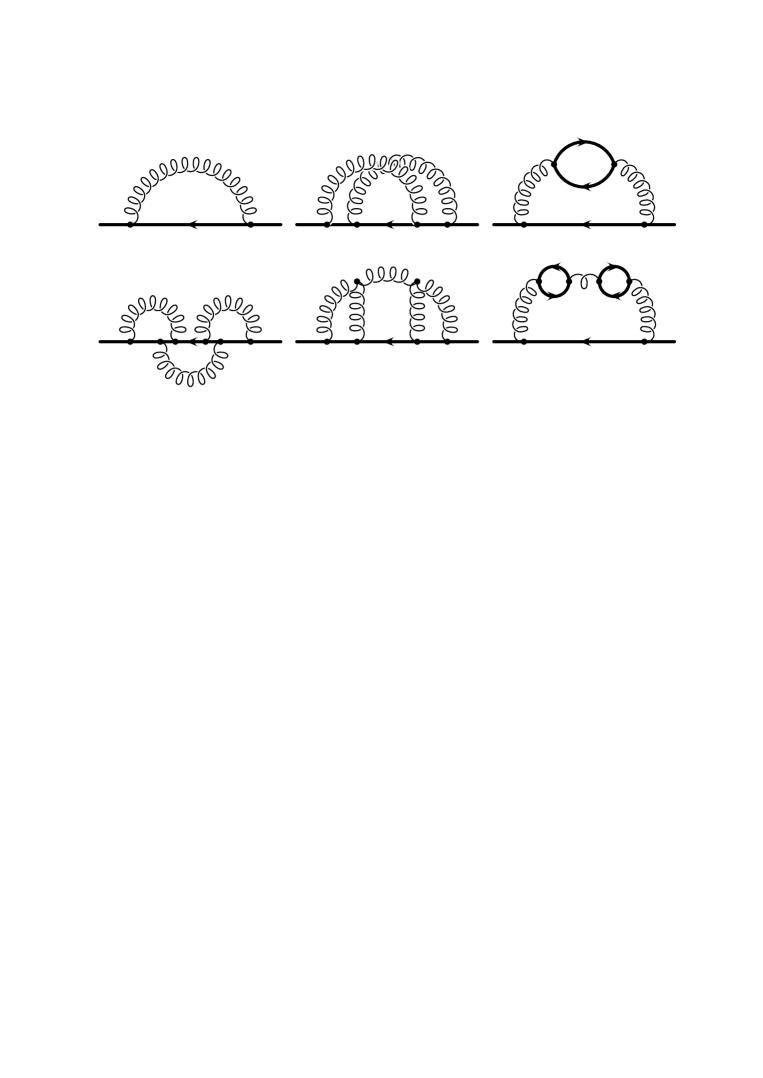
Figure 1: Sample diagrams contributing to the fermion propagator. The fermions in the closed loops may either also carry mass $M$ or considered to be massless.

Let us summarize the strategy for the practical computation: The scalar and vector part of the one-, two- and three-loop fermion propagator is computed. Afterwards we construct with the help of the $\overline{\rm MS}$ renormalization constants $Z_{2}$ and $Z_{m}$ and the two-loop relation between the $\overline{\rm MS}$ and the on-shell mass the finite functions $S_{S}(z)$ and $S_{V}(z)$. The proper combination according to Eqs. (15) serves as a convenient starting point to apply the conformal mapping (13) and subsequently the Padé approximation in order to obtain numerical results for the coefficients $z_{m}^{X}$ at the scale $\mu^{2}=M^{2}$. The use of the renormalization group equation leads to expression for different choices of $\mu^{2}$.

As our approach relies on approximations some words concerning the error estimate are in order. Even at three-loop order seven terms both in the small- and large-momentum expansion could be evaluated. Thus we restrict ourselves to those Padé results which include at least terms of order $z^{5}$ and $1/z^{4}$. Furthermore we require that the difference of the polynomial in the numerator and denominator is not too large, i.e. we select those Padé results which are close to the diagonal ones. From the results we compute the average and from the spread the error is estimated. The details will be specified below. In the next Section we will demonstrate that this prescription works very well at one- and two-loop order.

4 Considerations at one- and two-loop level

Let us at this point discuss the one- and two-loop results in great detail in order to get some feeling about the numerical quality of our procedure. In a first step we consider Feynman gauge and demonstrate afterwards how the results can be improved by considering a general gauge parameter.

In Tab. 1 the results for different Padé approximations are listed. $n$ indicates the number of low-energy moments involved in the analysis, i.e. $n=6$ implies the inclusion of terms of ${\cal O}(z^{6})$. The number of high-energy terms can be obtained in combination with the order of the Padé approximant ($[x/y]$) and is given by $x+y+1-n$.

$n$	P.A.	$F$	$FF$	$FA$	$FL$	$FH$
$5$	$[4/5]$	${}^{\star}-1.0010$	$-0.4881$	$-3.3813$	${}^{\star}1.5687$	$-0.1613$
$5$	$[4/6]$	$-1.0006$	$-0.4862$	${}^{\star}-3.4099$	$1.5666$	$-0.0811$
$5$	$[5/4]$	$-1.0008$	$-0.4870$	$-3.3936$	$1.5676$	$-0.1600$
$5$	$[5/5]$	$-1.0006$	$-0.4862$	$-3.3699$	$1.5663$	${}^{\star}-0.1616$
$5$	$[5/6]$	$-1.0002$	${}^{\star}-0.4884$	—	$1.5638$	${}^{\star}-0.1534$
$5$	$[6/4]$	$-1.0006$	$-0.4862$	$-3.3884$	$1.5665$	$-0.1381$
$5$	$[6/5]$	—	${}^{\star}-0.4884$	${}^{\star}-3.3972$	—	${}^{\star}-0.1526$
$6$	$[4/6]$	$-1.0007$	${}^{\star}-0.4888$	$-3.3148$	$1.5668$	${}^{\star}-0.1608$
$6$	$[5/5]$	$-1.0006$	$-0.4910$	$-3.3628$	$1.5665$	${}^{\star}-0.1561$
$6$	$[5/6]$	$-1.0002$	${}^{\star}-0.4866$	${}^{\star}-3.4084$	$1.5640$	${}^{\star}-0.1545$
$6$	$[5/7]$	$-1.0003$	$-0.4938$	${}^{\star}-3.3824$	$1.5646$	${}^{\star}-0.1572$
$6$	$[6/4]$	$-1.0007$	$-0.4894$	${}^{\star}-3.3830$	$1.5667$	$-0.1382$
$6$	$[6/5]$	—	${}^{\star}-0.4865$	${}^{\star}-3.4208$	—	${}^{\star}-0.1543$
$6$	$[6/6]$	$-1.0003$	${}^{\star}-0.4897$	—	$1.5646$	—
$6$	$[7/5]$	$-1.0004$	—	$-3.3777$	$1.5648$	${}^{\star}-0.1576$

Table 1: Results for the one- and two-loop coefficients of $z_{m}$. $n$ indicates the number of moments included into the analysis. Padé approximations which develop a pole for $|\omega|<1$ are represented by a dash. Those where a cancellation with the numerator takes place (see text) are marked by a star ($\star$). For the gauge parameter $\xi=0$ has been adopted.

Some Padé approximants develop poles inside the unit circle ($|\omega|\leq 1$). In general we will discard such results in the following and represent the results by a dash. In some cases, however, the pole coincides with a zero of the numerator up to several digits accuracy. These Padé approximations will be marked by a star ($\star$) and will be taken into account in constructing our results. To be precise: in addition to the Padé results without any poles inside the unit circle, we will use the ones where the poles are accompanied by zeros within a circle of radius 0.01, and the distance between the pole and the physically relevant point $q^{2}/M^{2}=1$ is larger than 0.1.

The exact values are given in Eqs. (8). At first sight good agreement is obtained in all five cases. A closer look shows that at order $\alpha_{s}$ almost all results are consistently below the exact value. However, the maximal deviation is far below the per mille level. Similar observations can be made in the case of the light-fermion corrections at order $\alpha_{s}^{2}$ which are proportional to $C_{F}Tn_{l}$. Here the deviation from the exact result amount to a few per mille. The spread in the $C_{F}^{2}$ term at two-loop order amounts to about 1%, however, the exact result is not covered. The deviation is small and well below 2%. For the structure $C_{F}C_{A}$ the error is smaller and the correct result lies inside the interval.

The situation is less pleasant for the $FH$ part. Strong fluctuations are observed in Tab. 1. It seems that there is a significant influence from the threshold at $q^{2}=9M^{2}$ which has the consequence that no stabilization is observed if higher order terms in the large-$z$ expansion are incorporated into the Padé analysis. Under these circumstances it is very promising, as was already mentioned above, to ignore the high-energy terms completely and compute the Padé approximations including only the knowledge from $z\to 0$. In this case a conformal mapping is not mandatory and the computation can also directly be performed in the variable $z$. The results can be found in Tab. 2 where the Padé results which develop poles inside the unit circle are again represented by a dash.

$n$	P.A.	$FH-z$	$FH-\omega$
$4$	$[1/3]$	$-0.1552$	$-0.1556$
$4$	$[2/2]$	$-0.1553$	$-0.1551$
$4$	$[3/1]$	$-0.1553$	—
$4$	$[4/0]$	$-0.1552$	$0.0114$
$5$	$[1/4]$	$-0.1553$	$-0.1552$
$5$	$[2/3]$	$-0.1553$	$-0.1553$
$5$	$[3/2]$	$-0.1553$	$-0.1553$
$5$	$[4/1]$	$-0.1553$	—
$5$	$[5/0]$	$-0.1553$	$-0.3222$
$6$	$[1/5]$	$-0.1553$	$-0.1554$
$6$	$[2/4]$	$-0.1553$	$-0.1554$
$6$	$[3/3]$	$-0.1553$	$-0.1555$
$6$	$[4/2]$	$-0.1553$	$-0.1554$
$6$	$[5/1]$	$-0.1553$	$-0.1568$
$6$	$[6/0]$	$-0.1553$	$0.0061$

Table 2: Results for the structure $FH$ where only low-energy moments have been incorporated. Only in the case of “$FH-\omega$” a conformal mapping has been used.

Note that all possible Padé approximants are included — even the simple Taylor expansions which correspond to the Padés with degree zero in the denominator. Both the stability and the agreement with the exact result is very impressive in the case where no conformal mapping is performed. In the case with conformal mapping the Taylor expansions show large oscillations. However, the other results nicely group around the exact value with an uncertainty in the per mille level. For the choice $\mu^{2}=M^{2}$ the threshold at $q^{2}=M^{2}$ is very much suppressed as compared to the one at $q^{2}=9M^{2}$. This is the reason that $z$ is a very good expansion parameter for $z\to 0$ and the sole inclusion of the low-energy terms leads to an excellent agreement with the exact value. Thus for $FH$ we discard the results presented in Tab. 1 and take the ones of Tab. 2 where the Padé approximation was performed in the variable $z$.

At this point some comments in connection with the Padé method are in order. The final values for the mean and the errors actually depend on the Padé approximants included into the analysis. In Tab. 1 only those results are incorporated which involve $z^{5}$, respectively, $z^{6}$ terms and corrections of order $1/z^{4}$, $1/z^{5}$ or $1/z^{6}$ from the high energy expansion. We also demand that the difference in the degree of the polynomial in the numerator and denominator is less or equal to two. If one of these conditions is loosened the size of the error would only slightly increase and the range would then cover the exact value. Furthermore one should remember that only information from small and large external momenta enter into the Padé analysis. The numerical values, however, are extracted for $q^{2}=M^{2}$. They arise from combinations of different pieces where each one exhibits singularities at threshold. Thus, in general one can not expect that an agreement up to three or more digits with the exact result can be found.

For the construction of the results in Tab. 1 the same input information was used which will be available at three-loop order. At one- and two-loop level, however, more moments can be computed. In Tab. 3 results are shown where terms up to order $z^{8}$, respectively, $1/z^{8}$ are incorporated. Indeed, the general tendency is a slight reduction in the error for all colour factors.

$n$	P.A.	$F$	$FF$	$FA$	$FL$	$FH$
$7$	$[6/7]$	—	${}^{\star}-0.4954$	${}^{\star}-3.3596$	${}^{\star}1.5643$	—
$7$	$[6/8]$	$-1.0002$	${}^{\star}-0.4926$	${}^{\star}-3.4026$	$1.5638$	${}^{\star}-0.1542$
$7$	$[7/6]$	$-1.0003$	${}^{\star}-0.4953$	${}^{\star}-3.3603$	$1.5641$	$-0.1555$
$7$	$[7/7]$	$-1.0002$	${}^{\star}-0.4925$	${}^{\star}-3.4088$	$1.5638$	${}^{\star}-0.1541$
$7$	$[7/8]$	—	$-0.4945$	$-3.3722$	—	${}^{\star}-0.1517$
$7$	$[8/6]$	$-1.0002$	${}^{\star}-0.4926$	${}^{\star}-3.3998$	$1.5638$	${}^{\star}-0.1541$
$7$	$[8/7]$	${}^{\star}-1.0003$	—	—	${}^{\star}1.5644$	${}^{\star}-0.1288$
$8$	$[6/8]$	$-1.0002$	${}^{\star}-0.4930$	$-3.3073$	$1.5639$	$-0.1552$
$8$	$[7/7]$	$-1.0002$	—	—	$1.5638$	$-0.1552$
$8$	$[7/8]$	—	${}^{\star}-0.4945$	—	—	$-0.1551$
$8$	$[7/9]$	$-1.0001$	$-0.4991$	${}^{\star}-3.3593$	$1.5632$	$-0.1554$
$8$	$[8/6]$	$-1.0002$	${}^{\star}-0.4943$	—	$1.5639$	$-0.1552$
$8$	$[8/7]$	${}^{\star}-1.0003$	${}^{\star}-0.4936$	—	${}^{\star}1.5646$	${}^{\star}-0.1547$
$8$	$[8/8]$	$-1.0001$	$-0.4989$	${}^{\star}-3.3607$	$1.5632$	$-0.1554$
$8$	$[9/7]$	$-1.0002$	$-0.4993$	${}^{\star}-3.3594$	$1.5633$	$-0.1557$

Table 3: Results for the one- and two-loop coefficients where terms up to order $z^{8}$, respectively, $1/z^{8}$ are incorporated.

As compared to Tab. 1 the situation for FH becomes quite different. The inclusion of more low-energy moments leads to significantly more stable results. Note, however, that at three-loop order the input data for $n=7$ and $n=8$ are not available which means that for the diagrams of such type we follow the strategy outlined above.

At three-loop level the moments are only available up to order $z^{6}$, respectively, $1/z^{6}$. The results obtained with these input data (cf. Tabs. 1 and 2) read [2]

$$\begin{array}[]{lll}\displaystyle z_{m}^{F}\,\,=\,\,-1.0005(8)\,,&\displaystyle z_{m}^{FF}\,\,=\,\,-0.49(1)\,,&\displaystyle z_{m}^{FA}\,\,=\,\,-3.4(1)\,,\\ &\displaystyle z_{m}^{FL}\,\,=\,\,1.566(5)\,,&z_{m}^{FH}\,\,=\,\,-0.1553(2)\,.\end{array}$$ (18)

where the error is obtained by doubling the spread of the different Padé approximants. The comparison with the exact result results [6] $\{-1$, $-0.51056$, $-3.33026$, $1.56205$, $-0.15535\}$ shows very good agreement — except for the structure $FF$ where our error estimate is off by a factor of two. We will come back to that point below after considering the general-$\xi$ results.

Up to now the discussion was based on Feynman gauge only, which corresponds to $\xi=0$ in our notation. In the remaining part of this section we allow for a general gauge parameter and demonstrate how the results of Eq. (18) can be improved. At one- and two-loop level only the colour structures $C_{F}$, $C_{F}^{2}$ and $C_{F}C_{A}$ develop a $\xi$ dependence. The proper combination of the self energies which contributes to the relation between the on-shell and $\overline{\rm MS}$ mass evaluated at $z=1$ must be independent of the specific choice of $\xi$. On the other hand, the expansion terms actually depend on the QCD gauge parameter, $\xi$. As we are dealing with a finite number of terms we are left with a residual $\xi$ dependence in the final result. It is clear that for extreme values of $\xi$ any predictive power of our procedure gets lost as the coefficients of $\xi$ become dominant. However, the final values should be stable against small variations around $\xi=0$. Thus it is worth to examine the dependence on $\xi$.

$n$ P.A. $F$ $FF$ $FA$ $5$ $[4/5]$ ${}^{\star}-0.9982$ $-0.4644$ $-3.4939$ $5$ $[4/6]$ $-0.9989$ $-0.4618$ $-3.2830$ $5$ $[5/4]$ $-0.9986$ $-0.4596$ ${}^{\star}-3.2273$ $5$ $[5/5]$ $-0.9990$ $-0.4673$ $-3.3145$ $5$ $[5/6]$ $-0.9996$ ${}^{\star}-0.4617$ $-3.2547$ $5$ $[6/4]$ $-0.9989$ $-0.4629$ $-3.2604$ $5$ $[6/5]$ — ${}^{\star}-0.4616$ $-3.2570$ $6$ $[4/6]$ $-0.9988$ ${}^{\star}-0.4468$ $-3.2946$ $6$ $[5/5]$ $-0.9989$ $-0.4770$ $-3.3044$ $6$ $[5/6]$ $-0.9995$ ${}^{\star}-0.4574$ $-3.2613$ $6$ $[5/7]$ $-0.9994$ $-0.4721$ ${}^{\star}-3.2672$ $6$ $[6/4]$ $-0.9989$ $-0.4670$ $-3.2513$ $6$ $[6/5]$ — ${}^{\star}-0.4561$ $-3.2675$ $6$ $[6/6]$ $-0.9994$ ${}^{\star}-0.4518$ ${}^{\star}-3.2837$ $6$ $[7/5]$ $-0.9994$ $-0.4739$ ${}^{\star}-3.2628$

$n$ P.A. $F$ $FF$ $FA$ $5$ $[4/5]$ — $-0.5105$ — $5$ $[4/6]$ $-1.0000$ $-0.5040$ $-3.3521$ $5$ $[5/4]$ $-1.0000$ $-0.5105$ $-3.3531$ $5$ $[5/5]$ $-1.0000$ ${}^{\star}-0.5209$ $-3.3499$ $5$ $[5/6]$ $-1.0000$ ${}^{\star}-0.5100$ ${}^{\star}-3.3521$ $5$ $[6/4]$ $-1.0000$ $-0.5055$ $-3.3517$ $5$ $[6/5]$ ${}^{\star}-1.0000$ ${}^{\star}-0.5099$ ${}^{\star}-3.3521$ $6$ $[4/6]$ $-1.0000$ $-0.5070$ ${}^{\star}-3.3576$ $6$ $[5/5]$ $-1.0000$ ${}^{\star}-0.5119$ — $6$ $[5/6]$ $-1.0000$ ${}^{\star}-0.5093$ ${}^{\star}-3.3540$ $6$ $[5/7]$ $-1.0000$ ${}^{\star}-0.5114$ $-3.3472$ $6$ $[6/4]$ $-1.0000$ $-0.5083$ $-3.3497$ $6$ $[6/5]$ ${}^{\star}-1.0000$ ${}^{\star}-0.5092$ ${}^{\star}-3.3545$ $6$ $[6/6]$ $-1.0000$ ${}^{\star}-0.5112$ ${}^{\star}-3.3557$ $6$ $[7/5]$ $-1.0000$ ${}^{\star}-0.5115$ $-3.3464$

Table 4: Results for the structures $F$, $FF$ and $FA$ where for the gauge parameter the values $\xi=-5$ (left table) and $\xi=-2$ (right table) have been adopted.

$n$ P.A. $F$ $FF$ $FA$ $5$ $[4/5]$ ${}^{\star}-1.0021$ $-0.4344$ $-3.3930$ $5$ $[4/6]$ $-1.0013$ ${}^{\star}-0.4176$ ${}^{\star}-3.4638$ $5$ $[5/4]$ $-1.0017$ $-0.4209$ $-3.4105$ $5$ $[5/5]$ $-1.0013$ $-0.4473$ $-3.3778$ $5$ $[5/6]$ $-1.0005$ ${}^{\star}-0.4212$ ${}^{\star}-3.4175$ $5$ $[6/4]$ $-1.0013$ $-0.4286$ $-3.4050$ $5$ $[6/5]$ — ${}^{\star}-0.4206$ ${}^{\star}-3.4195$ $6$ $[4/6]$ $-1.0014$ — $-3.3301$ $6$ $[5/5]$ $-1.0013$ $-0.4597$ — $6$ $[5/6]$ $-1.0006$ ${}^{\star}-0.4099$ ${}^{\star}-3.4389$ $6$ $[5/7]$ $-1.0007$ $-0.4397$ ${}^{\star}-3.3990$ $6$ $[6/4]$ $-1.0014$ $-0.4353$ ${}^{\star}-3.3972$ $6$ $[6/5]$ — ${}^{\star}-0.4024$ ${}^{\star}-3.4692$ $6$ $[6/6]$ $-1.0007$ ${}^{\star}-0.2736$ ${}^{\star}-3.2798$ $6$ $[7/5]$ $-1.0008$ $-0.4444$ $-3.3914$

$n$ P.A. $F$ $FF$ $FA$ $5$ $[4/5]$ ${}^{\star}-1.0039$ $-0.3230$ $-3.3834$ $5$ $[4/6]$ $-1.0024$ — ${}^{\star}-3.4196$ $5$ $[5/4]$ $-1.0030$ $-0.2620$ $-3.3970$ $5$ $[5/5]$ $-1.0022$ $-0.3700$ $-3.3713$ $5$ $[5/6]$ $-1.0009$ ${}^{\star}-0.2110$ ${}^{\star}-3.4006$ $5$ $[6/4]$ $-1.0023$ — $-3.3917$ $5$ $[6/5]$ — ${}^{\star}-0.1970$ ${}^{\star}-3.4017$ $6$ $[4/6]$ $-1.0025$ $-0.4670$ $-3.3204$ $6$ $[5/5]$ $-1.0024$ $-0.3853$ $-3.3643$ $6$ $[5/6]$ $-1.0010$ ${}^{\star}-0.0740$ ${}^{\star}-3.4146$ $6$ $[5/7]$ $-1.0013$ ${}^{\star}-0.2749$ ${}^{\star}-3.3856$ $6$ $[6/4]$ $-1.0025$ ${}^{\star}-0.3001$ ${}^{\star}-3.3857$ $6$ $[6/5]$ — — ${}^{\star}-3.4305$ $6$ $[6/6]$ $-1.0012$ ${}^{\star}-0.5118$ — $6$ $[7/5]$ $-1.0014$ $-0.3122$ $-3.3803$

Table 5: Results for the structures $F$, $FF$ and $FA$ where for the gauge parameter the values $\xi=+2$ (left table) and $\xi=+5$ (right table) have been adopted.

In Tabs. 4 and 5 the results are shown for the $F$, $FF$ and $FA$ structures where the values $\xi=\pm 5$ and $\xi=\pm 2$ have been adopted. The one-loop result is quite stable against the variation of $\xi$ and even for $\xi=\pm 5$ the deviations to the exact result is small. Also the results for $C_{A}C_{F}$ exhibit a quite small variation for the different values of $\xi$. Only the structure $FF$ shows larger deviations from the exact value if $\xi$ is varied. Especially the average value for $\xi=+5$ is off by roughly 40%. However, one also has to take into account that in this case the procedure seems to be less stable and the errors are larger. A closer look into the results for the expansion terms shows that for this choice the coefficients of the $z^{n}$ terms are already dominated by the $\xi$-dependent terms whereas, for instance, for $\xi=-5$ this is not the case.

For all colour structures the best results are obtained for the choice $\xi=-2$. This can be understood with the help of the following considerations. As is well known [36] the QED fermion propagator get infra-red finite (in the leading log approximation) in a particular gauge, namely for $\xi=-2$ in our notation (cf. Eq. (9)). Thus, it is not surprising that for this particular choice our approximate results for $z_{m}$ demonstrate better convergence to the known ones. It also suggests that the use of the same gauge condition ($\xi=-2$) should lead to better results at least for the QED parts of $z_{m}$ at three-loop order. This will be discussed in detail in Section 6.

Figure 2: $z$ dependence of $-g(z)$ for the structures $F$, $FF$ and $FA$ for different values of $\xi$. The solid curves belong to $\xi=-2$. The dashed curves correspond to $\xi=-5,0,+2,+5$ (from short to long dashes).

In Fig. 2 the structures $F$, $FF$ and $FA$ of the function $-g(z)$ are plotted for five different values of $\xi$. In each figure ten different curves are plotted — two different Padé results for each value of $\xi$. Whereas for $z\not=1$ the single curves show a quite different behaviour there is the tendency to converge to the same value for $z=1$ which corresponds to the respective coefficient of $z_{m}$. For comparison also the result for $FL$ is shown in Fig. 2 which has no $\xi$ dependence at all and which agrees with the exact result within 0.3%. In the case of $F$ all curves are smooth at the point $z=1$ which is reflected in the impressive stability shown in Tabs. 1, 4 and 5. On the contrary, for most values of $\xi$ the two-loop structures $FF$ and $FA$ exhibit a kink for $z=1$. In the case of $FF$ even the sign of the derivative is different for $z<1$ and $z>1$ and a relatively strong variation around $z=1$ is observed. A closer look shows that the value $\xi=-2$ obviously represents an exception. For this choice the curves exhibit the smoothest behaviour around $z=1$. This is also reflected in the numbers presented in Tab. 4 which are most stable for $\xi=-2$. Actually the structure $FF$ has stronger singularities at threshold for $\xi=0$ than the other coefficients which explains the deviation from the exact result in Eq. (18). Thus it is suggestive to choose $\xi=-2$ in order to extract the results:

$$\begin{array}[]{lll}\displaystyle z_{m}^{F}\,\,=\,\,-1.0000(0)\,,&\displaystyle z_{m}^{FF}\,\,=\,\,-0.51(2)\,,&\displaystyle z_{m}^{FA}\,\,=\,\,-3.35(1)\,,\end{array}$$ (20)

where the errors were obtained in the same way as before. We would like to stress that there is an impressive agreement with the exact results (cf. Eq. (8)).

Despite the fact that the uncertainties in Eqs. (20) are quite small the total error would be significantly overestimated if one would naively add the contributions from the individual colour factors. Instead it is more promising to add the moments in a first step (of course, taking into account the correct colour factors) and performing the conformal mapping and Padé approximation afterwards. The results for the quantity

$$z_{m}^{(2),light}(n_{l}) = C_{F}^{2}z_{m}^{FF}+C_{F}C_{A}z_{m}^{FA}+C_{F}Tn_{l}z_{m}^{FL}\,$$ (21)

for different choices of $n_{l}$ can be found in Tabs. 6 and 7 where the gauge parameter has been fixed to $\xi=0$ and $\xi=-2$, respectively. In both cases the spread among the different results is very small. Using again twice the spread of the different Padé approximants as an estimate for the error we get for $\xi=0$

$$z_{m}^{(2),light}(0)=-14.4(6)\,, z_{m}^{(2),light}(1)=-13.3(6)\,, z_{m}^{(2),light}(2)=-12.3(4)\,,$$

$$z_{m}^{(2),light}(3)=-11.2(5)\,, z_{m}^{(2),light}(4)=-10.2(3)\,, z_{m}^{(2),light}(5)=-9.1(3)\,.$$ (22)

Good agreement with the exact results, which are listed in the last column of the tables, is obtained. For $\xi=-2$ the following results can be extracted

$$z_{m}^{(2),light}(0)=-14.3(2)\,, z_{m}^{(2),light}(1)=-13.2(2)\,, z_{m}^{(2),light}(2)=-12.2(2)\,,$$

$$z_{m}^{(2),light}(3)=-11.1(1)\,, z_{m}^{(2),light}(4)=-10.07(3)\,, z_{m}^{(2),light}(5)=-9.02(1)\,.$$ (23)

Here the error is slightly reduced and is well below 2%.

$n$	P.A.	$n_{l}=0$	$n_{l}=1$	$n_{l}=2$	$n_{l}=3$	$n_{l}=4$	$n_{l}=5$
$5$	$[4/5]$	$-14.3431$	$-13.2932$	$-12.2433$	$-11.1933$	$-10.1432$	$-9.0931$
$5$	$[4/6]$	$-14.2673$	$-13.2188$	$-12.1700$	$-11.1206$	$-10.0703$	$-9.0183$
$5$	$[5/4]$	$-14.3816$	$-13.3305$	$-12.2791$	$-11.2273$	$-10.1750$	$-9.1221$
$5$	$[5/5]$	$-14.3188$	$-13.2702$	$-12.2216$	$-11.1730$	$-10.1244$	$-9.0758$
$5$	$[5/6]$	${}^{\star}-14.7124$	${}^{\star}-13.5777$	${}^{\star}-12.4638$	${}^{\star}-11.3641$	${}^{\star}-10.2745$	${}^{\star}-9.1925$
$5$	$[6/4]$	${}^{\star}-14.4299$	${}^{\star}-13.3703$	${}^{\star}-12.3109$	${}^{\star}-11.2517$	${}^{\star}-10.1927$	${}^{\star}-9.1340$
$5$	$[6/5]$	—	—	—	${}^{\star}-11.4712$	${}^{\star}-10.3346$	${}^{\star}-9.2264$
$6$	$[4/6]$	$-14.2802$	$-13.2344$	$-12.1885$	$-11.1425$	$-10.0963$	$-9.0499$
$6$	$[5/5]$	$-14.3149$	$-13.2662$	$-12.2176$	$-11.1689$	$-10.1203$	$-9.0717$
$6$	$[5/7]$	${}^{\star}-14.5630$	${}^{\star}-13.4629$	${}^{\star}-12.3745$	${}^{\star}-11.2942$	${}^{\star}-10.2200$	${}^{\star}-9.1502$
$6$	$[6/4]$	${}^{\star}-14.3676$	${}^{\star}-13.3163$	${}^{\star}-12.2647$	${}^{\star}-11.2130$	${}^{\star}-10.1610$	${}^{\star}-9.1088$
$6$	$[6/5]$	$-14.2190$	$-13.1684$	$-12.1164$	$-11.0623$	$-10.0043$	$-8.9382$
$6$	$[6/6]$	${}^{\star}-14.2867$	${}^{\star}-13.2389$	${}^{\star}-12.1910$	${}^{\star}-11.1431$	${}^{\star}-10.0951$	${}^{\star}-9.0469$
$6$	$[7/5]$	$-14.3713$	$-13.3191$	$-12.2668$	$-11.2142$	$-10.1613$	$-9.1082$
	exact	$-14.2287$	$-13.1874$	$-12.146$	$-11.1046$	$-10.0633$	$-9.02188$

Table 6: Results for $z_{m}^{(2),light}(n_{l})$ for different values of $n_{l}$. The gauge parameter has been fixed to $\xi=0$.

$n$	P.A.	$n_{l}=0$	$n_{l}=1$	$n_{l}=2$	$n_{l}=3$	$n_{l}=4$	$n_{l}=5$
$5$	$[4/5]$	$-14.2809$	$-13.2304$	$-12.1797$	$-11.1284$	$-10.0754$	${}^{\star}-9.0136$
$5$	$[4/6]$	$-14.1864$	—	—	${}^{\star}-11.1492$	${}^{\star}-10.0769$	$-9.0194$
$5$	$[5/4]$	$-14.3044$	$-13.2494$	$-12.1933$	$-11.1360$	$-10.0771$	$-9.0164$
$5$	$[5/5]$	$-14.2670$	$-13.2184$	$-12.1698$	$-11.1212$	$-10.0726$	$-9.0245$
$5$	$[5/6]$	${}^{\star}-14.3356$	${}^{\star}-13.2670$	${}^{\star}-12.2014$	${}^{\star}-11.1382$	${}^{\star}-10.0769$	${}^{\star}-9.0173$
$5$	$[6/4]$	${}^{\star}-14.3073$	${}^{\star}-13.2492$	$-12.1913$	$-11.1336$	$-10.0760$	$-9.0186$
$5$	$[6/5]$	${}^{\star}-14.3458$	${}^{\star}-13.2720$	${}^{\star}-12.2035$	${}^{\star}-11.1387$	${}^{\star}-10.0769$	${}^{\star}-9.0173$
$6$	$[4/6]$	$-14.2460$	$-13.1986$	$-12.1504$	$-11.0983$	${}^{\star}-10.0940$	$-9.0191$
$6$	$[5/5]$	$-14.2625$	$-13.2139$	$-12.1653$	$-11.1167$	$-10.0677$	$-9.0202$
$6$	$[5/6]$	—	${}^{\star}-13.3253$	${}^{\star}-12.2248$	${}^{\star}-11.1461$	${}^{\star}-10.0785$	$-9.0172$
$6$	$[5/7]$	${}^{\star}-14.3106$	${}^{\star}-13.2490$	${}^{\star}-12.1892$	${}^{\star}-11.1309$	$-10.0737$	${}^{\star}-9.0177$
$6$	$[6/4]$	${}^{\star}-14.2928$	${}^{\star}-13.2394$	${}^{\star}-12.1853$	${}^{\star}-11.1306$	$-10.0748$	$-9.0179$
$6$	$[6/5]$	—	—	${}^{\star}-12.2729$	${}^{\star}-11.1535$	${}^{\star}-10.0790$	$-9.0175$
$6$	$[6/6]$	${}^{\star}-14.2375$	${}^{\star}-13.1871$	${}^{\star}-12.1322$	—	${}^{\star}-10.0819$	${}^{\star}-9.0177$
$6$	$[7/5]$	$-14.2909$	$-13.2370$	$-12.1827$	$-11.1280$	$-10.0731$	${}^{\star}-9.0177$
	exact	$-14.2287$	$-13.1874$	$-12.146$	$-11.1046$	$-10.0633$	$-9.02188$

Table 7: Results for $z_{m}^{(2),light}(n_{l})$ for different values of $n_{l}$. The gauge parameter has been fixed to $\xi=-2$.

In summary, very good agreement with the exact results for the different coefficients of $z_{m}$ are observed at one- and two-loop order. The results obtained from the fifth and sixth low-energy moment and a high-energy expansion up to ${\cal O}(1/z^{6})$ suggests that also at order $\alpha_{s}^{3}$ it is possible to get reliable results. The analysis for different values of $\xi$ showed that the choice $\xi=-2$ would be the preferable one. However, also $\xi=0$ leads to very good results. At three-loop order the calculation for general $\xi$ is only possible for some of the diagrams, namely the ones which are already present in QED. For those diagrams, which have stronger singularities for $z=1$, $\xi=-2$ will be adopted. In the remaining cases the results are obtained for $\xi=0$. In the approach where the moments are added in a first step our method provides for $\xi=0$ results which are in very good agreement with the exact ones.

5 Master integrals

Before we go on to the discussion of the three-loop results the technology behind the practical calculation shall be discussed in more detail. The high-energy expansion can be reduced to the evaluation of massless propagator-type diagrams up to three loops and one- and two-loop vacuum graphs. The relevant tools are available since quite some time (see, e.g., [37]). The technology needed in the limit $z\to 0$, however, has never been applied to real processes. Furthermore the discussion in the literature is not complete. In this Section we review the knowledge about vacuum graphs and close the gaps.

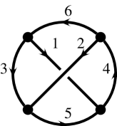
Figure 3: Generic three-loop bubble diagram. In general each line may be massless or carry mass $M$.

The computation of the three-loop diagrams in the limit of vanishing external momentum reduces to the evaluation of vacuum graphs as shown in Fig. 3 with one dimensionful scale given by the mass, $M$. In principle each line may be massless or carry mass $M$. The general strategy to compute such kind of diagrams is based on the integration-by-parts method [38]. It provides recurrence relations which are used in order to express complicated integrals in terms of simple ones and a small set of a few so-called master integrals for which a real integration is necessary. Those master integrals, however, only have to be computed once and forever.

The recurrence relations and master integrals which are necessary for the computation of ${\cal O}(\alpha_{s}^{2})$ corrections to the $\gamma$ and $Z$ boson propagator have been considered in [39]. In this case only one difficult integral had to be solved. It is shown in Fig. 4(e). In [40] the technique has been extended to the case of the $W$ boson. Altogether only three difficult master integrals are necessary for the evaluation of the gauge boson self energies. In addition to the one in Fig. 4(e) also the diagrams in Fig. 4(c) and Fig. 5(b) have to be taken into account.

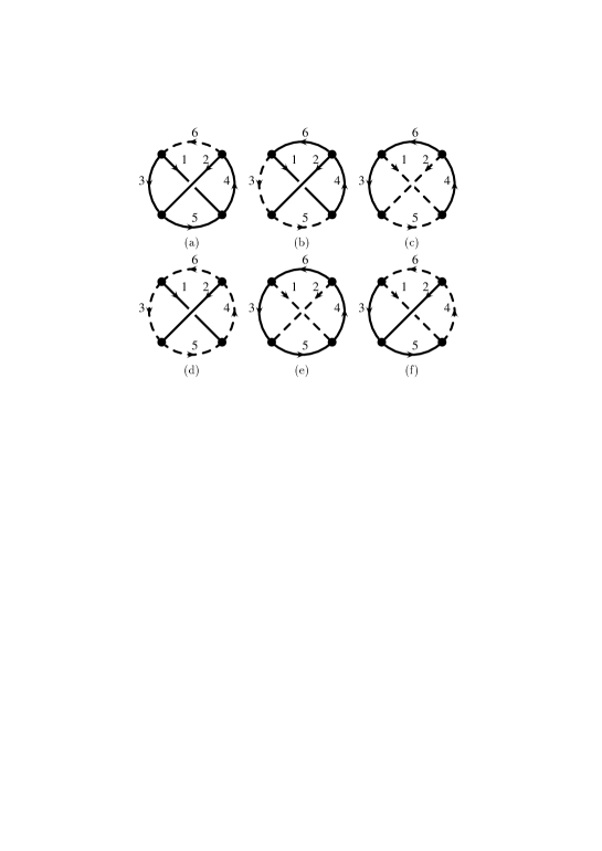
Figure 4: Master diagrams corresponding to the expression in Eq. (25). The full lines carry mass $M$ whereas the dashed ones are massless.

(a)	(b)	(c)

Figure 5: Two- and three-loop master diagrams corresponding to the expressions in Eqs. (27) and (5). The full lines carry mass $M$ whereas the dashed ones are massless.

For the fermion propagator the variety of integrals to be computed at three-loop level is larger as there are more choices whether a certain line of the three-loop tadpole diagram shown in Fig. 3 may be massive or massless. Let us collect all master integrals which are needed for the computation of the moments for the fermion propagator. It is convenient to introduce the following function

$$M_{n_{1},n_{2},n_{6}}(M_{1},\ldots,M_{6})=$$

$$\mbox{}\int\frac{{\rm d}^{D}p\,{\rm d}^{D}k\,{\rm d}^{D}l}{(M^{2}\pi)^{3D/2}}\frac{M^{6+2n_{1}+2n_{2}+2n_{6}}}{(p_{1}^{2}+M_{1}^{2})^{n_{1}}(p_{2}^{2}+M_{2}^{2})^{n_{2}}(p_{3}^{2}+M_{3}^{2})(p_{4}^{2}+M_{4}^{2})(p_{5}^{2}+M_{5}^{2})(p_{6}^{2}+M_{6}^{2})^{n_{6}}}\,,$$

where the masses $M_{i}$ are either equal to $M$ or zero. $D=4-2\varepsilon$ is the space-time dimension. The factors of $M^{2}$ have been introduced in order to make the function $M(\ldots)$ dimensionless. The momenta $p_{i}$ are linear combinations of the integration momenta $p$, $k$ and $l$. In [41] the recurrence relations for those mass decompositions were derived which were not discussed in [39]. They can be used in order to arrive at the master integrals pictured in Fig. 4. The results can be found in [39, 42]

$$M_{111}(M,M,M,M,M,0) = \frac{2\zeta_{3}}{\varepsilon}+6\zeta_{3}-\frac{469}{27}\zeta_{4}+\frac{8}{3}\left[{\rm Cl}_{2}\left(\frac{\pi}{3}\right)\right]^{2}$$

$$\mbox{}-16\sum_{m>n>0}\frac{(-1)^{m}\cos(2\pi n/3)}{m^{3}n}$$

$$\approx \frac{2\zeta_{3}}{\varepsilon}-8.2168598175087380629133983386010858249695\,,$$

$$M_{111}(M,M,0,M,0,M) = \frac{2\zeta_{3}}{\varepsilon}+6\zeta_{3}-\frac{77}{12}\zeta_{4}-6\left[{\rm Cl}_{2}\left(\frac{\pi}{3}\right)\right]^{2}\,,$$

$$M_{111}(0,0,M,M,0,M) = \frac{2\zeta_{3}}{\varepsilon}+6\zeta_{3}-\frac{15}{4}\zeta_{4}-6\left[{\rm Cl}_{2}\left(\frac{\pi}{3}\right)\right]^{2}\,,$$

$$M_{111}(M,M,0,0,0,0) = \frac{2\zeta_{3}}{\varepsilon}+6\zeta_{3}-\frac{21}{2}\zeta_{4}-4\zeta_{2}\ln^{2}2+\frac{2}{3}\ln^{4}2+16{\rm Li}_{4}\left(\frac{1}{2}\right)\,,$$

$$M_{111}(0,0,M,M,M,M) = \frac{2\zeta_{3}}{\varepsilon}+6\zeta_{3}-22\zeta_{4}-8\zeta_{2}\ln^{2}2+\frac{4}{3}\ln^{4}2+32{\rm Li}_{4}\left(\frac{1}{2}\right)\,,$$

$$M_{111}(0,M,M,0,M,0) = \frac{2\zeta_{3}}{\varepsilon}+6\zeta_{3}-\frac{11}{2}\zeta_{4}-4\left[{\rm Cl}_{2}\left(\frac{\pi}{3}\right)\right]^{2}\,,$$ (25)

where $\zeta_{n}$ is Rieman’s zeta function with the values $\zeta_{2}=\pi^{2}/6$, $\zeta_{3}\approx 1.20205690$ and $\zeta_{4}=\pi^{4}/90$. ${\rm Cl}_{2}(x)$ is the Clausen function and ${\rm Li}_{4}(x)$ represents the quadrilogarithm. The order of the expressions listed in Eq. (25) agrees with the one of Fig. 4(a)–(f). Note that the case where all six lines are massive does not occur for the three-loop QCD corrections to the quark propagator.

It is interesting to note that the results corresponding to Figs. 4(a) and (e) can be obtained from the ${\cal O}(\varepsilon)$ part of the diagrams where the index of one of the massless lines is reduced to zero using the integration-by-parts technique. The resulting topology leads to much simpler expressions as it can essentially be written as a product of two one-loop integrals with an additional integration over the corresponding external momentum. For the other four cases the topologies presented in Fig. 4 have to be considered in order to reproduce the results of Eq. (25). The reason for this is that the absence of any of the lines immediately leads to (in general simpler) integrals which at the end result in different master integrals.

In the practical application of the recurrence relations it turns out that except the master integrals of Eq. (25) also the one of Fig. 5(c) is needed. Furthermore the ${\cal O}(D-4)$ parts of the diagram pictured in Fig. 5(b) is required. These pieces will be provided in the following.

For their practical computation it is convenient to consider integrals which are less divergent. This is achieved by doubling some of the propagators. In the case of Fig. 5(b) we double each of the massive propagators and for Fig. 5(c) the propagators corresponding to line 1, 2 and 4 are raised to power two. This leads us to ultra-violet convergent integrals. The infra-red divergence introduced in the latter case does not spoil the evaluation. It manifests itself as as single $1/\varepsilon$ pole in the final result. In a next step we introduce Feynman parameters and thus combine the different denominators. Then the momentum integrations can be carried out and one ends up with two- (Fig. 5(b)), respectively, three-dimensional (Fig. 5(c)) integral representations. In each case the leading terms of order $1/\varepsilon$, respectively, $\varepsilon^{0}$ can be used in order to check the constants which are already known. The expansion up to next-to-leading order in $\varepsilon$ provides the structures we are interested in. In both cases one ends up with a one-dimensional integration where the most difficult integrals look like:

$$\int_{0}^{1}{\rm d}x\frac{x^{n}\ln(x)\ln(1-x+x^{2})}{(1-x+x^{2})^{2}}\,,\qquad n=0,1,\ldots\,.$$ (26)

The integration can be performed analytically and finally leads to the following results for the master integrals:

$$M_{001}(0,0,M,M,0,M) = \frac{1}{\varepsilon^{3}}+\frac{15}{4\varepsilon^{2}}+\frac{1}{\varepsilon}\left(\frac{65}{8}+\frac{3}{2}\zeta_{2}\right)+\frac{135}{16}+\frac{45}{8}\zeta_{2}-\zeta_{3}$$

$$\mbox{}+3\sqrt{3}{\rm Cl}_{2}\left(\frac{\pi}{3}\right)+\varepsilon\left(-\frac{763}{32}-\frac{9\sqrt{3}\pi}{16}\ln^{2}3-\frac{35\sqrt{3}\pi^{3}}{48}\right.$$

$$\left.\mbox{}+\frac{195}{16}\zeta_{2}-\frac{15}{4}\zeta_{3}+\frac{57}{16}\zeta_{4}+\frac{45\sqrt{3}}{2}{\rm Cl}_{2}\left(\frac{\pi}{3}\right)\right.$$

$$\left.\mbox{}-27\sqrt{3}{\rm Im}\left[{\rm Li}_{3}\left(\frac{e^{-i\pi/6}}{\sqrt{3}}\right)\right]\right)\,,$$

$$M_{110}(0,M,M,0,M,0) = -\frac{2}{3\varepsilon^{3}}-\frac{11}{3\varepsilon^{2}}+\frac{1}{\varepsilon}\left(-14-2\zeta_{2}+2\sqrt{3}{\rm Cl}_{2}\left(\frac{\pi}{3}\right)\right)$$ (27)

$$\mbox{}-\frac{139}{3}-\frac{\sqrt{3}\pi}{8}\ln^{2}3-\frac{17\sqrt{3}\pi^{3}}{72}-\frac{21}{2}\zeta_{2}+\frac{1}{3}\zeta_{3}$$

$$\mbox{}+10\sqrt{3}{\rm Cl}_{2}\left(\frac{\pi}{3}\right)-6\sqrt{3}{\rm Im}\left[{\rm Li}_{3}\left(\frac{e^{-i\pi/6}}{\sqrt{3}}\right)\right]\,.$$

These expressions were used in [2] and coincide with the results listed in a recent work [43].

As an outcome of the recurrence relations also products of one- and two-loop integrals may appear. This makes in necessary to evaluate also the ${\cal O}(\varepsilon)$ part of the two-loop diagram shown in Fig. 5(a). A straightforward Feynman parametrisation gives (in agreement with [44]):

$$T(M,M,M) = \int\frac{{\rm d}^{D}p{\rm d}^{D}k}{(M^{2}\pi)^{D}}\frac{M^{6}}{(p^{2}+M^{2})(k^{2}+M^{2})((p+k)^{2}+M^{2})}$$

$$= -\frac{3}{2\varepsilon^{2}}-\frac{9}{2\varepsilon}-\frac{21}{2}-\frac{3}{2}\zeta_{2}+2\sqrt{3}{\rm Cl}_{2}\left(\frac{\pi}{3}\right)+\varepsilon\left(-\frac{45}{2}-\frac{\sqrt{3}\pi}{8}\ln^{2}3\right.$$

$$\left.\mbox{}-\frac{35\sqrt{3}\pi^{3}}{216}-\frac{9}{2}\zeta_{2}+\zeta_{3}+6\sqrt{3}{\rm Cl}_{2}\left(\frac{\pi}{3}\right)-6\sqrt{3}{\rm Im}\left[{\rm Li}_{3}\left(\frac{e^{-i\pi/6}}{\sqrt{3}}\right)\right]\right)\,.$$

All other integrals which have to solved are of one- and two-loop tadpole type. The two-loop integrals are similar to the ones of Eq. (5), however, one or two lines are massless. For these kind of integrals there exists a solution valid to any order in $\varepsilon$ and for arbitrary exponents of the propagators in the denominator.

A numerical check of the integrals in Eqs. (25) has been performed. A straightforward Feynman parameterization leads to multidimensional integrals for which a Monte Carlo integration routine [45] has been used in order to obtain 5 significant digits.

As an independent check of the results for the diagrams pictured in Fig. 5 the following method was used: One of the massive lines is cut in such a way that the remaining two-loop diagram has a threshold starting from $4M^{2}$. Then the mass of the cut line is set to $M^{\prime}$ and an asymptotic expansion for $M^{\prime}\ll M$ is performed. The effective expansion parameter is $(M^{\prime})^{2}/(4M^{2})$. Thus is very suggestive that even for $M^{\prime}=M$ a reasonably fast approximation to the exact result can be expected. Actually the first 20 expansion terms for the diagrams in Fig. 5 reproduce the first 10 digits of the exact result. Note that it only makes sense to apply this method if the diagram which results from the original one after setting the mass of the selected line to zero is computable analytically.

6 Three-loop results

In this section the results of order $\alpha_{s}^{3}$ are discussed. Altogether 131 diagrams contribute. The evaluation in the limit $z\to 0$ reduces to a naive Taylor expansion in the external momentum. Thus one ends up with three-loop vacuum integrals where the computation follows closely the lines of Section 5. In the limit of large external momentum the rules of asymptotic expansion (see, e.g., Refs. [46, 37] for reviews) have to be applied. As a result for each diagram several subgraphs have to be considered which leads to roughly 3500 diagrams to be evaluated. It is clear that this cannot be done by hand and the use of computer algebra becomes unavoidable. The practical calculation has been performed with the package GEFICOM [47]. It calls the programs LMP [28], respectively, EXP [48] in order to perform the asymptotic expansion. A recent summary of the available software can be found in [37]. In both limits we were able to evaluate the first seven terms in the expansion, i.e. terms up to ${\cal O}(z^{6})$ and ${\cal O}(1/z^{6})$, respectively, are available. Thereby Feynman gauge has been adopted.

In principle the expansion terms of the colour structures $FFF$, $FFA$, $FFL$, $FFH$, $FAA$, $FAL$ und $FAH$ depend on the QCD gauge parameter, $\xi$. The remaining three structures contain two closed fermion loops and thus $\xi$ drops out at an early stage of the calculation. A straightforward computation of the $\xi$-dependent terms produces huge expressions in intermediate steps and leads quite fast to the limitations set by the soft- and hardware. For the abelian case there exists a simple Ward identity which allows a very fast calculation of the $\xi$-dependent part of the fermion propagator [49]

$$\frac{d}{d\xi}S_{F}^{0,QED}(q) = -e_{0}^{2}\int\frac{d^{D}p}{i(2\pi)^{D}}\frac{1}{p^{4}}S_{F}^{0,QED}(q-p)\,.$$ (29)

Within dimensional regularization Eq. (29) is an exact equation which relates the $\xi$-dependent part of the fermion propagator in $L+1$-loop order with the full propagator at $L$-loop order. In fact, the calculation of the r.h.s. of (29) for general gauge is significantly faster than that of the very function $S_{F}^{QED}$ in (the simplest) Feynman gauge. This is because of the “factorizable” nature of the integration with respect to the momentum $p$.

Using Eq. (29) we have computed the ($\xi$-dependent) QED colour structures $FFF$, $FFL$ and $FFH$. To our best knowledge there is not a simple generalization of the identity (29) for QCD, i.e. the non-abelian contributions. Thus the results for the corresponding colour factors can only be analyzed for $\xi=0$.

Let us in a first step discuss the results for $\xi=0$ and afterwards consider the QED-like diagrams for general $\xi$.

In Tabs. 8 and 9 the results for the individual colour structures can be found where $\xi=0$ has been adopted for the gauge parameter. Only those results are listed which include at least the terms of ${\cal O}(z^{5})$ and ${\cal O}(1/z^{4})$. Furthermore we require that the difference of the degree of the polynomial in the numerator and denominator is less or equal to two. The Padé approximations which develop poles inside the unit plane and where no appropriate cancellation takes place are again represented by a dash.

$n$	P.A.	$FFF$	$FFA$	$FFL$	$FFH$	$FAA$
$5$	$[4/5]$	$2.0338$	$-2.0665$	$0.7347$	$2.4876$	$-16.2692$
$5$	$[4/6]$	$2.0272$	$-2.0031$	$0.7341$	$2.5147$	${}^{\star}-16.4584$
$5$	$[5/4]$	$2.0310$	$-2.0632$	$0.7371$	$2.4752$	$-16.3826$
$5$	$[5/5]$	$2.0263$	$-1.9981$	$0.7343$	$2.5057$	$-16.4243$
$5$	$[5/6]$	$2.1191$	${}^{\star}-1.9318$	${}^{\star}0.7379$	$2.5305$	${}^{\star}-16.4890$
$5$	$[6/4]$	$2.0344$	$-2.0025$	$0.7325$	$2.5623$	$-16.4381$
$5$	$[6/5]$	$2.1091$	${}^{\star}-1.8018$	$0.7421$	$2.5281$	${}^{\star}-16.4903$
$6$	$[4/6]$	$2.0236$	${}^{\star}-2.0587$	$0.7411$	$2.4954$	$-16.3748$
$6$	$[5/5]$	$2.0220$	$-2.0457$	$0.7423$	$2.4951$	$-16.3949$
$6$	$[5/6]$	${}^{\star}1.9686$	${}^{\star}-2.0304$	${}^{\star}0.7372$	$2.5188$	${}^{\star}-16.4554$
$6$	$[5/7]$	${}^{\star}2.0648$	${}^{\star}-2.0962$	$0.7601$	$1.1897$	—
$6$	$[6/4]$	$2.0234$	$-1.9897$	$0.7410$	$2.4984$	$-16.4185$
$6$	$[6/5]$	$2.2334$	${}^{\star}-2.0243$	${}^{\star}0.7392$	$2.5182$	${}^{\star}-16.4689$
$6$	$[6/6]$	${}^{\star}2.0548$	${}^{\star}-2.0858$	$0.7653$	${}^{\star}2.6713$	${}^{\star}-16.4411$
$6$	$[7/5]$	${}^{\star}2.1493$	${}^{\star}-2.1205$	$0.7567$	$2.3704$	$-16.3435$

Table 8: Three-loop results for $z_{m}^{X}$ ($X=FFF,FFA,FFL,FFH,FAA$) for $\xi=0$. The same notation as in Tab. 1 has been adopted.

$n$	P.A.	$FAL$	$FAH$	$FLL$	$FLH$	$FHH$
$5$	$[4/5]$	—	${}^{\star}-1.4898$	${}^{\star}-1.9890$	$-0.0630$	$-0.1806$
$5$	$[4/6]$	$13.4932$	$-1.3224$	—	$-0.0708$	$-0.1958$
$5$	$[5/4]$	${}^{\star}13.6711$	$-1.5551$	${}^{\star}-1.9764$	$-0.0601$	$-0.1669$
$5$	$[5/5]$	$13.4519$	${}^{\star}-1.5357$	—	$-0.0686$	$-0.1948$
$5$	$[5/6]$	${}^{\star}13.7944$	${}^{\star}-1.5136$	${}^{\star}-2.0122$	$-0.0703$	—
$5$	$[6/4]$	$13.5259$	$-1.4147$	—	$-0.0824$	$-0.3390$
$5$	$[6/5]$	${}^{\star}13.6020$	${}^{\star}-1.5133$	$-1.9646$	$-0.0690$	—
$6$	$[4/6]$	$13.3826$	${}^{\star}-1.5250$	${}^{\star}-1.9937$	$-0.0662$	$-0.1939$
$6$	$[5/5]$	$13.3533$	${}^{\star}-1.5254$	${}^{\star}-1.9985$	$-0.0660$	$-0.1930$
$6$	$[5/6]$	$12.9396$	${}^{\star}-1.5183$	$-1.9767$	$-0.0695$	$-0.1928$
$6$	$[5/7]$	$13.3481$	—	$-1.9696$	$-0.0486$	$-0.1887$
$6$	$[6/4]$	$13.4640$	$-1.4777$	${}^{\star}-1.9981$	$-0.0676$	$-0.2154$
$6$	$[6/5]$	—	${}^{\star}-1.5173$	—	$-0.0695$	$-0.1928$
$6$	$[6/6]$	$13.3138$	—	$-1.9698$	$-0.0319$	$-0.1911$
$6$	$[7/5]$	$13.4209$	—	$-1.9693$	$-0.0542$	$-0.1880$

Table 9: Three-loop results for $z_{m}^{X}$ ($X=FAL,FAH,FLL,FLH,FHH$) for $\xi=0$. The same notation as in Tab. 1 has been adopted.

Very nice agreement between the different values in each column of Tabs. 8 and  9 can be found. There is one obvious exception in the structure FFH namely the $[5/7]$ Padé approximation where the sixth moment was used for the construction. A closer look shows that there is a pole close to $z=1$ ($\omega=1.105\ldots$, respectively, $z=0.997\ldots$) which explains the deviation from the other results. In order to obtain the final numbers we will not take this value into account.

From Tab. 9 one observes that the structures $FLH$ and $FHH$ are less stable than the others. The reason for this is the same as for $FH$ at two-loop order. Again the threshold at $q^{2}=M^{2}$ is suppressed as compared to the one at $q^{2}=9M^{2}$ which suggests that the expansion around $z=0$ should provide a reasonable expansion parameter. In Tab. 10 the results for these two colour structures where no high energy terms were used are shown. Actually almost all Padé approximants performed in the variable $\omega$ develop poles for $|\omega|<1$. Thus we decided not to use them for our analysis. In analogy to the two-loop case the results are very stable and only a small differences between the naive Taylor expansion and diagonal Padé results are observed. Thus in the following the results of Tab. 10 are used for the structures $FLH$ and $FHH$.

$n$	P.A.	$FFHz$	$FAHz$	$FLHz$	$FHHz$
$4$	$[1/3]$	$2.4135$	$-1.5047$	$-0.0669$	$-0.1922$
$4$	$[2/2]$	$2.4135$	${}^{\star}-1.4790$	$-0.0670$	$-0.1922$
$4$	$[3/1]$	$2.4065$	$-1.5042$	$-0.0670$	$-0.1922$
$4$	$[4/0]$	$2.3531$	$-1.494$	$-0.0673$	$-0.1922$
$5$	$[1/4]$	$2.4310$	$-1.5085$	$-0.0669$	$-0.1922$
$5$	$[2/3]$	${}^{\star}2.4143$	$-1.5103$	$-0.0669$	$-0.1922$
$5$	$[3/2]$	$2.4364$	$-1.5102$	$-0.0668$	$-0.1922$
$5$	$[4/1]$	$2.4236$	$-1.5080$	$-0.0669$	$-0.1922$
$5$	$[5/0]$	$2.3765$	$-1.4990$	$-0.0671$	$-0.1922$
$6$	$[1/5]$	$2.4410$	$-1.5109$	$-0.0668$	$-0.1922$
$6$	$[2/4]$	$2.4473$	$-1.5126$	${}^{\star}-0.0669$	$-0.1922$
$6$	$[3/3]$	$2.4488$	$-1.5120$	$-0.0668$	$-0.1922$
$6$	$[4/2]$	$2.4474$	$-1.5126$	$-0.0668$	$-0.1922$
$6$	$[5/1]$	$2.4352$	$-1.5105$	$-0.0668$	$-0.1922$
$6$	$[6/0]$	$2.3933$	$-1.5024$	$-0.0669$	$-0.1922$

Table 10: Results for the colour structures involving a closed heavy fermion loop. Only the moments for $z\to 0$ have been implemented into the Padé analysis.

It is tempting to consider also for the colour factors $C_{F}^{2}T$ and $C_{F}C_{A}T$ the results which exclusively contain the information from the expansion around $z\to 0$. They are also displayed in Tab. 10. There is perfect agreement with the numbers extracted from Tabs. 8 and 9, the errors, however, are significantly smaller. Thus we decided to take also for these colour structures the results of Tab. 10.

Finally we get the following results if $\xi=0$ is adopted:

$$\begin{array}[]{lll}\displaystyle z_{m}^{FFF}\,\,=\,\,2.1(3)\,,&\displaystyle z_{m}^{FFA}\,\,=\,\,-2.0(4)\,,&\displaystyle z_{m}^{FFL}\,\,=\,\,0.74(4)\,,\\ \displaystyle z_{m}^{FFH}\,\,=\,\,2.4(1)\,,&z_{m}^{FAA}\,\,=\,\,-16.4(3)\,,&z_{m}^{FAL}\,\,=\,\,13(1)\,,\\ z_{m}^{FAH}\,\,=\,\,-1.51(5)\,,&z_{m}^{FLL}\,\,=\,\,-1.98(6)\,,&z_{m}^{FLH}\,\,=\,\,-0.0669(6)\,,\\ z_{m}^{FHH}\,\,=\,\,-0.1922(0)\,,\end{array}$$ (34)

where the error has again been obtained by doubling the spread of the Padé approximants.

Let us now analyze the QED-like diagrams, i.e. the structures $FFF$, $FFL$ and $FFH$ for arbitrary gauge parameter. In analogy to the one- and two-loop case considered in Section 4 we vary $\xi$ between $-5$ and $+5$. The corresponding results can be found in Tabs. 11 and 12.

$n$ P.A. $FFF$ $FFL$ $FFH$ $5$ $[4/5]$ $2.1093$ $1.0402$ $2.5059$ $5$ $[4/6]$ $2.0926$ $1.0354$ $2.4652$ $5$ $[5/4]$ $2.1082$ $1.0430$ $2.5013$ $5$ $[5/5]$ $2.0923$ ${}^{\star}1.0443$ $2.4650$ $5$ $[5/6]$ ${}^{\star}1.5554$ $1.0229$ $3.1456$ $5$ $[6/4]$ $2.0954$ $1.0193$ $2.4717$ $5$ $[6/5]$ $2.6737$ $1.0230$ $2.8145$ $6$ $[4/6]$ $2.0985$ ${}^{\star}1.0540$ $2.4565$ $6$ $[5/5]$ $2.1016$ ${}^{\star}1.0602$ $2.4248$ $6$ $[5/6]$ ${}^{\star}2.0780$ $1.0016$ ${}^{\star}2.4470$ $6$ $[5/7]$ ${}^{\star}2.1475$ ${}^{\star}1.0204$ ${}^{\star}2.5472$ $6$ $[6/4]$ $2.1000$ $1.0283$ $2.4623$ $6$ $[6/5]$ ${}^{\star}2.0498$ $1.0103$ ${}^{\star}2.3488$ $6$ $[6/6]$ ${}^{\star}2.1400$ ${}^{\star}1.0278$ ${}^{\star}2.5325$ $6$ $[7/5]$ ${}^{\star}2.1828$ ${}^{\star}1.0118$ ${}^{\star}2.6241$

$n$ P.A. $FFF$ $FFL$ $FFH$ $5$ $[4/5]$ $2.0599$ $0.8596$ $2.4949$ $5$ $[4/6]$ $2.0447$ $0.8527$ $2.4978$ $5$ $[5/4]$ $2.0580$ $0.8599$ $2.4865$ $5$ $[5/5]$ $2.0444$ $0.8549$ $2.4932$ $5$ $[5/6]$ $2.3098$ $0.8545$ $2.5776$ $5$ $[6/4]$ $2.0489$ $0.8468$ $2.5242$ $5$ $[6/5]$ $2.2055$ $0.8558$ $2.5769$ $6$ $[4/6]$ $2.0434$ — $2.4867$ $6$ $[5/5]$ $2.0369$ ${}^{\star}0.8575$ $2.4863$ $6$ $[5/6]$ ${}^{\star}2.0280$ $0.8534$ $2.5959$ $6$ $[5/7]$ ${}^{\star}2.0854$ $0.8568$ ${}^{\star}2.5867$ $6$ $[6/4]$ $2.0441$ $0.8537$ $2.4863$ $6$ $[6/5]$ ${}^{\star}1.9423$ $0.8535$ $2.5567$ $6$ $[6/6]$ ${}^{\star}2.0777$ $0.8570$ ${}^{\star}2.5503$ $6$ $[7/5]$ ${}^{\star}2.1340$ $0.8569$ ${}^{\star}3.5102$

Table 11: Results for the structures $FFF$, $FFL$ and $FFH$ where for the gauge parameter the values $\xi=-5$ (left table) and $\xi=-2$ (right table) have been adopted.

$n$ P.A. $FFF$ $FFL$ $FFH$ $5$ $[4/5]$ $1.9184$ $0.6080$ $2.4799$ $5$ $[4/6]$ $1.8976$ $0.6182$ $2.5284$ $5$ $[5/4]$ $1.9030$ $0.6138$ $2.4614$ $5$ $[5/5]$ $1.8970$ $0.6187$ $2.5146$ $5$ $[5/6]$ $1.9309$ ${}^{\star}0.6178$ $2.5105$ $5$ $[6/4]$ $1.9061$ $0.6187$ $2.6074$ $5$ $[6/5]$ $1.9309$ ${}^{\star}0.6267$ $2.5030$ $6$ $[4/6]$ $1.8906$ $0.6384$ $2.5005$ $6$ $[5/5]$ $1.8878$ $0.6557$ $2.4993$ $6$ $[5/6]$ — ${}^{\star}0.6091$ $2.5076$ $6$ $[5/7]$ ${}^{\star}1.9425$ $0.6720$ $2.4446$ $6$ $[6/4]$ $1.8897$ $0.6311$ $2.5098$ $6$ $[6/5]$ $1.9346$ ${}^{\star}0.6175$ $2.5075$ $6$ $[6/6]$ ${}^{\star}1.9248$ $0.6886$ $2.4268$ $6$ $[7/5]$ ${}^{\star}3.0282$ $0.6587$ $2.4514$

$n$ P.A. $FFF$ $FFL$ $FFH$ $5$ $[4/5]$ $0.9431$ $0.4164$ $2.4671$ $5$ $[4/6]$ $1.2669$ $0.4493$ $2.5427$ $5$ $[5/4]$ $1.3734$ $0.4280$ $2.4317$ $5$ $[5/5]$ $1.2631$ $0.4558$ $2.5229$ $5$ $[5/6]$ $1.2435$ ${}^{\star}0.4313$ $2.4983$ $5$ $[6/4]$ $1.2642$ $0.4492$ $2.7025$ $5$ $[6/5]$ $1.2325$ ${}^{\star}0.4503$ $2.4846$ $6$ $[4/6]$ $1.2467$ $0.5049$ $2.5046$ $6$ $[5/5]$ $1.2236$ $0.6468$ $2.5022$ $6$ $[5/6]$ $1.2332$ ${}^{\star}0.3972$ $2.5029$ $6$ $[5/7]$ $1.1881$ $0.5539$ $2.4788$ $6$ $[6/4]$ $1.2428$ $0.4712$ $2.5305$ $6$ $[6/5]$ $1.2510$ ${}^{\star}0.4210$ $2.5020$ $6$ $[6/6]$ $1.1799$ $0.5975$ $2.4780$ $6$ $[7/5]$ $1.1955$ $0.5159$ $2.4782$

Table 12: Results for the structures $FFF$, $FFL$ and $FFH$ where for the gauge parameter the values $\xi=+2$ (left table) and $\xi=+5$ (right table) have been adopted.

In the case $FFH$ we actually prefer to use only the low-energy moments. The corresponding results for $\xi=-5,-2,0,+2$ and $+5$ can be found in Tab. 13. For all choices very stable results with a spread below 3% are obtained. Furthermore they are all consistent with each other.

$n$	P.A.	$\xi=-5$	$\xi=-2$	$\xi=+2$	$\xi=+5$
$4$	$[1/3]$	$2.4174$	$2.4145$	$2.4135$	$2.4161$
$4$	$[2/2]$	$2.4182$	$2.4146$	$2.4135$	$2.4162$
$4$	$[3/1]$	$2.4165$	$2.4102$	$2.4032$	$2.3985$
$4$	$[4/0]$	$2.3648$	$2.3578$	$2.3484$	$2.3414$
$5$	$[1/4]$	$2.4336$	$2.4317$	$2.4306$	$2.4304$
$5$	$[2/3]$	$2.4271$	${}^{\star}2.4204$	${}^{\star}2.4029$	—
$5$	$[3/2]$	$2.4436$	$2.4386$	$2.4345$	$2.4319$
$5$	$[4/1]$	$2.4298$	$2.4259$	$2.4215$	$2.4184$
$5$	$[5/0]$	$2.3847$	$2.3798$	$2.3733$	$2.3684$
$6$	$[1/5]$	$2.4423$	$2.4413$	$2.4408$	$2.4406$
$6$	$[2/4]$	$2.4478$	$2.4474$	$2.4478$	$2.4525$
$6$	$[3/3]$	$2.4525$	$2.4497$	$2.4485$	$2.4526$
$6$	$[4/2]$	$2.4523$	$2.4490$	$2.4460$	$2.4441$
$6$	$[5/1]$	$2.4394$	$2.4368$	$2.4337$	$2.4315$
$6$	$[6/0]$	$2.3992$	$2.3957$	$2.3909$	$2.3873$

Table 13: Results for $FFH$ where only the low-energy moments are taken into account. Different choices for the gauge parameter are adopted.

It is instructive to examine also at three-loop order the $z$ dependence around $z=1$ for different values of $\xi$ which is done in Fig. 6 for the $\xi$-dependent colour structures $FFF$, $FFL$ and $FFH$. The result for $FLL$ which does not depend on $\xi$ is plotted for comparison. Actually the corresponding part of the function $-g(z)$ is plotted in the vicinity of $z=1$. The ten curves in each plot correspond to $\xi=-5,-2,0,+2$ and $\xi=+5$ where for each value of $\xi$ two different Padé results are shown.

It can be seen that as for the order $\alpha_{s}$ and $\alpha_{s}^{2}$ cases also here the choice $\xi=-2$ (solid curve) exhibits the smoothest behaviour for $z=1$ which was already expected from the stable behaviour of the numbers in Tabs. 11 and 12. Thus it can be expected that for this values our procedure works best. However, we want to stress that — in analogy to the lower order analysis — the value $\xi=0$ looks very promising and also for this choice reasonable results can be expected.

Adopting the choice $\xi=-2$ we extract from Tabs. 11 and 13 the following results:

$$z_{m}^{FFF}=2.1(4)\,,\qquad z_{m}^{FFL}=0.8(2)\,,\qquad z_{m}^{FFH}=2.4(1)\,.$$ (35)

Note that the colour structure $FFL$ demonstrates a rather strong dependence on the gauge parameter. To take this into account we assigned somewhat extended errors to this quantity in Eq. (35).

Figure 6: $z$ dependence of $-g(z)$ for the structures $FFF$, $FFL$ and $FFH$ for different values of $\xi$. The solid curves belong to $\xi=-2$. The dashed curves correspond to $\xi=-5,0,+2,+5$ (from short to long dashes).

Note that the results of (34) and  (35) are valid for $\mu^{2}=M^{2}$. With the help of the two-loop $\beta$ [50] and three-loop $\gamma_{m}$ [51] function it is possible to restore the $\ln(\mu^{2}/M^{2})$ terms at order $\alpha_{s}^{3}$. Thus Eq. (1) reads

$$\frac{m(\mu)}{M} = 1+\frac{\alpha_{s}^{(n_{f})}(\mu)}{\pi}z_{m}^{(1)}(\mu)+\left(\frac{\alpha_{s}^{(n_{f})}(\mu)}{\pi}\right)^{2}z_{m}^{(2)}(\mu)+\left(\frac{\alpha_{s}^{(n_{f})}(\mu)}{\pi}\right)^{3}\Bigg{\{}z_{m}^{(3)}(M)+$$ (36)

$$\mbox{}C_{F}^{3}\left[-\frac{9}{128}l_{\mu M}^{3}-\frac{27}{128}l_{\mu M}^{2}+\left(-\frac{489}{512}+\frac{45}{32}\zeta_{2}-\frac{9}{4}\zeta_{2}\ln 2+\frac{9}{16}\zeta_{3}\right)l_{\mu M}\right]$$

$$\mbox{}+C_{F}^{2}C_{A}\left[\frac{33}{128}l_{\mu M}^{3}+\frac{109}{64}l_{\mu M}^{2}+\left(\frac{5813}{1536}-\frac{61}{16}\zeta_{2}+\frac{53}{8}\zeta_{2}\ln 2-\frac{53}{32}\zeta_{3}\right)l_{\mu M}\right]$$

$$\mbox{}+C_{F}^{2}Tn_{l}\left[-\frac{3}{32}l_{\mu M}^{3}-\frac{13}{32}l_{\mu M}^{2}+\left(\frac{65}{384}+\frac{7}{8}\zeta_{2}-2\zeta_{2}\ln 2-\frac{1}{4}\zeta_{3}\right)l_{\mu M}\right]$$

$$\mbox{}+C_{F}^{2}T\left[-\frac{3}{32}l_{\mu M}^{3}-\frac{13}{32}l_{\mu M}^{2}+\left(-\frac{151}{384}+2\zeta_{2}-2\zeta_{2}\ln 2-\frac{1}{4}\zeta_{3}\right)l_{\mu M}\right]$$

$$\mbox{}+C_{F}C_{A}^{2}\left[-\frac{121}{576}l_{\mu M}^{3}-\frac{2341}{1152}l_{\mu M}^{2}+\left(-\frac{13243}{1728}+\frac{11}{12}\zeta_{2}-\frac{11}{4}\zeta_{2}\ln 2+\frac{11}{16}\zeta_{3}\right)l_{\mu M}\right]$$

$$\mbox{}+C_{F}C_{A}Tn_{l}\left[\frac{11}{72}l_{\mu M}^{3}+\frac{373}{288}l_{\mu M}^{2}+\left(\frac{869}{216}+\frac{7}{12}\zeta_{2}+\zeta_{2}\ln 2+\frac{1}{2}\zeta_{3}\right)l_{\mu M}\right]$$

$$\mbox{}+C_{F}C_{A}T\left[+\frac{11}{72}l_{\mu M}^{3}+\frac{373}{288}l_{\mu M}^{2}+\left(\frac{583}{108}-\frac{13}{6}\zeta_{2}+\zeta_{2}\ln 2+\frac{1}{2}\zeta_{3}\right)l_{\mu M}\right]$$

$$\mbox{}+C_{F}T^{2}n_{l}^{2}\left[-\frac{1}{36}l_{\mu M}^{3}-\frac{13}{72}l_{\mu M}^{2}+\left(-\frac{89}{216}-\frac{1}{3}\zeta_{2}\right)l_{\mu M}\right]$$

$$\mbox{}+C_{F}T^{2}n_{l}\left[-\frac{1}{18}l_{\mu M}^{3}-\frac{13}{36}l_{\mu M}^{2}+\left(-\frac{143}{108}+\frac{1}{3}\zeta_{2}\right)l_{\mu M}\right]$$

$$\mbox{}+C_{F}T^{2}\left[-\frac{1}{36}l_{\mu M}^{3}-\frac{13}{72}l_{\mu M}^{2}+\left(-\frac{197}{216}+\frac{2}{3}\zeta_{2}\right)l_{\mu M}\right]\Bigg{\}}\,,$$

with $l_{\mu M}=\ln\mu^{2}/M^{2}$. $n_{f}=n_{l}+1$ is the number of active quark flavours. Very often the scale-invariant mass, $\mu_{m}$ defined through $\mu_{m}=m(\mu_{m})$ is of interest. Thus iterating (36) leads to

$$\frac{\mu_{m}}{M} = 1+\frac{\alpha_{s}^{(n_{f})}(M)}{\pi}z_{m}^{(1)}(M)+\left(\frac{\alpha_{s}^{(n_{f})}(M)}{\pi}\right)^{2}\left[z_{m}^{(2)}(M)+C_{F}^{2}\frac{3}{2}\right]+\left(\frac{\alpha_{s}^{(n_{f})}(M)}{\pi}\right)^{3}$$ (37)

$$\mbox{}\Bigg{[}z_{m}^{(3)}(M)+C_{F}^{3}\left(-\frac{741}{256}+\left(\frac{45}{16}-\frac{9}{2}\ln 2\right)\zeta_{2}+\frac{9}{8}\zeta_{3}\right)+C_{F}^{2}C_{A}\left(\frac{4885}{768}-\left(\frac{3}{4}\right.\right.$$

$$\left.\left.\mbox{}-\frac{9}{4}\ln 2\right)\zeta_{2}-\frac{9}{16}\zeta_{3}\right)+C_{F}^{2}T\left(-\frac{509}{192}+\frac{3}{2}\zeta_{2}\right)+C_{F}^{2}Tn_{l}\left(-\frac{293}{192}-\frac{3}{4}\zeta_{2}\right)\Bigg{]}\,.$$

Inverting Eq. (36) leads to

$$\frac{M}{m(\mu)} = 1+\frac{\alpha_{s}^{(n_{f})}(\mu)}{\pi}\left(-z_{m}^{(1)}(M)+\frac{3}{4}l_{\mu m}\right)+\left(\frac{\alpha_{s}^{(n_{f})}(\mu)}{\pi}\right)^{2}\Bigg{\{}-z_{m}^{(2)}(M)$$ (38)

$$\mbox{}+C_{F}^{2}\left[-\frac{1}{2}-\frac{9}{32}l_{\mu m}+\frac{9}{32}l_{\mu m}^{2}\right]+C_{F}C_{A}\left[\frac{185}{96}l_{\mu m}+\frac{11}{32}l_{\mu m}^{2}\right]$$

$$\mbox{}+C_{F}T\left(n_{l}+1\right)\left[-\frac{13}{24}l_{\mu m}-\frac{1}{8}l_{\mu m}^{2}\right]\Bigg{\}}$$

$$\mbox{}+\left(\frac{\alpha_{s}^{(n_{f})}(\mu)}{\pi}\right)^{3}\Bigg{\{}-z_{m}^{(3)}(M)+C_{F}^{3}\left[\frac{201}{256}+\left(\frac{15}{16}\zeta_{2}-\frac{3}{2}\ln 2\right)\zeta_{2}+\frac{3}{8}\zeta_{3}+\left(\frac{495}{512}\right.\right.$$

$$\left.\left.\mbox{}+\left(\frac{45}{32}-\frac{9}{4}\ln 2\right)\zeta_{2}+\frac{9}{16}\zeta_{3}\right)l_{\mu m}-\frac{63}{128}l_{\mu m}^{2}+\frac{9}{128}l_{\mu m}^{3}\right]+C_{F}^{2}C_{A}\left[-\frac{1849}{768}-\left(\frac{1}{4}\right.\right.$$

$$\left.\left.\mbox{}-\frac{3}{4}\ln 2\right)\zeta_{2}-\frac{3}{16}\zeta_{3}+\left(-\frac{4219}{1536}+\left(\frac{49}{16}-\frac{35}{8}\ln 2\right)\zeta_{2}+\frac{35}{32}\zeta_{3}\right)l_{\mu m}+\frac{21}{64}l_{\mu m}^{2}\right.$$

$$\left.\mbox{}+\frac{33}{128}l_{\mu m}^{3}\right]+C_{F}^{2}Tn_{l}\left[\frac{137}{192}-\frac{1}{4}\zeta_{2}+\left(-\frac{91}{384}+\zeta_{2}\left(-\frac{13}{8}+2\ln 2\right)+\frac{1}{4}\zeta_{3}\right)l_{\mu m}\right.$$

$$\left.\mbox{}-\frac{3}{32}l_{\mu m}^{2}-\frac{3}{32}l_{\mu m}^{3}\right]+C_{F}^{2}T\left[\frac{65}{192}+\frac{1}{2}\zeta_{2}+\left(-\frac{307}{384}+\zeta_{2}\left(-\frac{1}{2}+2\ln 2\right)\right.\right.$$

$$\left.\left.\mbox{}+\frac{1}{4}\zeta_{3}\right)l_{\mu m}-\frac{3}{32}l_{\mu m}^{2}-\frac{3}{32}l_{\mu m}^{3}\right]+C_{F}C_{A}^{2}\left[+\left(\frac{13243}{1728}+\left(-\frac{11}{12}+\frac{11}{4}\ln 2\right)\zeta_{2}\right.\right.$$

$$\left.\left.\mbox{}-\frac{11}{16}\zeta_{3}\right)l_{\mu m}+\frac{2341}{1152}l_{\mu m}^{2}+\frac{121}{576}l_{\mu m}^{3}\right]$$

$$\mbox{}+C_{F}C_{A}Tn_{l}\left[\left(-\frac{869}{216}-\left(\frac{7}{12}+\ln 2\right)\zeta_{2}-\frac{1}{2}\zeta_{3}\right)l_{\mu m}-\frac{373}{288}l_{\mu m}^{2}-\frac{11}{72}l_{\mu m}^{3}\right]$$

$$\mbox{}+C_{F}C_{A}T\left[\left(-\frac{583}{108}+\left(\frac{13}{6}-\ln 2\right)\zeta_{2}-\frac{1}{2}\zeta_{3}\right)l_{\mu m}-\frac{373}{288}l_{\mu m}^{2}-\frac{11}{72}l_{\mu m}^{3}\right]$$

$$\mbox{}+C_{F}T^{2}n_{l}^{2}\left[\left(\frac{89}{216}+\frac{1}{3}\zeta_{2}\right)l_{\mu m}+\frac{13}{72}l_{\mu m}^{2}+\frac{1}{36}l_{\mu m}^{3}\right]$$

$$\mbox{}+C_{F}T^{2}n_{l}\left[\left(\frac{143}{108}-\frac{1}{3}\zeta_{2}\right)l_{\mu m}+\frac{13}{36}l_{\mu m}^{2}+\frac{1}{18}l_{\mu m}^{3}\right]$$

$$\mbox{}+C_{F}T^{2}\left[\left(\frac{197}{216}-\frac{2}{3}\zeta_{2}\right)l_{\mu m}+\frac{13}{72}l_{\mu m}^{2}+\frac{1}{36}l_{\mu m}^{3}\right]\Bigg{\}}\,,$$

with $l_{\mu m}=\ln\mu^{2}/m^{2}(\mu)$.

If one is interested in the Eqs. (36), (37) or (38) the results of (34) and (35) can be used. However, for most practical applications only the values $N_{c}=3$, i.e. $C_{F}=4/3$ and $C_{A}=3$, and $T=1/2$ are of interest. Simply adding the results of the individual colour factors would lead to a big overestimation of the error. A closer look to the numbers in Eqs. (34) and (35) also indicates that once the numerical values for the colour factors and the number of light quarks are inserted numerical cancellations might occur which result in a loss of accuracy. Thus it is much more promising to add in a first step the results for the moments, of course, taking into account the proper colour factor. Afterwards the Padé approximations are computed. As the contributions with and without heavy quark loops are treated differently we consider the sum of both sets separately as a function of $n_{l}$. In Tab. 14 the results for the sum of the structures $FFF$, $FFA$, $FFL$, $FAA$, $FAL$ and $FLL$ is shown where $n_{l}$ is varied from 0 to 5. The analog combination of the remaining contributions ($FFH$, $FAH$, $FLH$, $FHH$) can be found in Tab. 15.

$n$	P.A.	$n_{l}=0$	$n_{l}=1$	$n_{l}=2$	$n_{l}=3$	$n_{l}=4$	$n_{l}=5$
$5$	$[4/5]$	$-200.2787$	$-173.6663$	$-148.3787$	$-124.4156$	$-101.7771$	$-80.4628$
$5$	$[4/6]$	$-201.6419$	$-174.8844$	$-149.4553$	$-125.3553$	$-102.5862$	$-81.1625$
$5$	$[5/4]$	$-203.9394$	$-176.7290$	$-150.8970$	$-126.4411$	$-103.3591$	$-81.6482$
$5$	$[5/5]$	$-201.4721$	$-174.7445$	$-149.3422$	$-125.2644$	$-102.5104$	$-81.0786$
$5$	$[5/6]$	$-198.7799$	$-172.8884$	$-148.2001$	—	${}^{\star}-102.2739$	${}^{\star}-81.0336$
$5$	$[6/4]$	$-202.8435$	$-175.8651$	$-150.2298$	$-125.9387$	$-102.9929$	$-81.3939$
$6$	$[4/6]$	$-201.0906$	$-174.3880$	$-149.0165$	$-124.9749$	$-102.2619$	$-80.8758$
$6$	$[5/5]$	$-200.9265$	$-174.2458$	$-148.8927$	$-124.8668$	$-102.1673$	$-80.7929$
$6$	$[5/6]$	${}^{\star}-200.4927$	${}^{\star}-173.9600$	${}^{\star}-148.7433$	${}^{\star}-124.8358$	${}^{\star}-102.2290$	${}^{\star}-80.9131$
$6$	$[5/7]$	$-200.3603$	$-173.7018$	$-148.3764$	$-124.3940$	$-101.7753$	$-80.5533$
$6$	$[6/4]$	$-201.6970$	$-174.9293$	$-149.4861$	$-125.3673$	$-102.5725$	$-81.1016$
$6$	$[6/6]$	$-200.3195$	$-173.6857$	$-148.3751$	$-124.3879$	$-101.7244$	$-80.3848$
$6$	$[7/5]$	$-202.1300$	$-175.2569$	$-149.7173$	$-125.5125$	$-102.6443$	$-81.1143$

Table 14: Padé results for the sum of those contributions which don’t have a closed heavy fermion loop. $n_{l}$ has been varied from 0 to 5.

$n$	P.A.	$n_{l}=0$	$n_{l}=1$	$n_{l}=2$	$n_{l}=3$	$n_{l}=4$	$n_{l}=5$
$4$	$[1/3]$	$-0.9345$	$-0.9572$	$-0.9798$	$-1.0024$	$-1.0249$	$-1.0475$
$4$	$[2/2]$	$-0.9321$	$-0.9546$	$-0.9770$	$-0.9995$	$-1.0218$	$-1.0442$
$4$	$[3/1]$	$-0.9324$	$-0.9551$	$-0.9777$	$-1.0003$	$-1.0229$	$-1.0455$
$4$	$[4/0]$	$-0.9604$	$-0.9828$	$-1.0053$	$-1.0277$	$-1.0501$	$-1.0725$
$5$	$[1/4]$	$-0.9271$	$-0.9495$	$-0.9720$	$-0.9944$	$-1.0169$	$-1.0393$
$5$	$[2/3]$	$-0.9219$	$-0.9440$	$-0.9661$	$-0.9882$	$-1.0103$	$-1.0324$
$5$	$[3/2]$	$-0.9086$	$-0.9347$	$-0.9591$	$-0.9827$	$-1.0060$	$-1.0290$
$5$	$[4/1]$	$-0.9254$	$-0.9478$	$-0.9703$	$-0.9927$	$-1.0151$	$-1.0375$
$5$	$[5/0]$	$-0.9495$	$-0.9719$	$-0.9942$	$-1.0166$	$-1.0389$	$-1.0613$
$6$	$[1/5]$	$-0.9217$	$-0.9441$	$-0.9665$	$-0.9888$	$-1.0112$	$-1.0336$
$6$	$[2/4]$	$-0.9140$	$-0.9364$	$-0.9589$	$-0.9813$	$-1.0037$	$-1.0261$
$6$	$[3/3]$	$-0.9125$	$-0.9352$	$-0.9578$	$-0.9803$	$-1.0028$	$-1.0252$
$6$	$[4/2]$	$-0.9126$	$-0.9352$	$-0.9578$	$-0.9803$	$-1.0028$	$-1.0253$
$6$	$[5/1]$	$-0.9202$	$-0.9425$	$-0.9649$	$-0.9872$	$-1.0096$	$-1.0319$
$6$	$[6/0]$	$-0.9416$	$-0.9639$	$-0.9862$	$-1.0085$	$-1.0308$	$-1.0532$

Table 15: Padé approximations performed in the variable $z$. No high-energy results have been used. Again $n_{l}$ has been varied from 0 to 5, the dependence, however, is very weak.

Using the results of Tabs. 14 and 15 with $n_{l}=0$ and $n_{l}$-dependent parts from Eqs. (34) and (35) the formulae (36), (37) and (38) can be written in the form

$$\frac{m(M)}{M} = 1-1.333a_{M}+a_{M}^{2}\left[-14.33+1.041n_{l}\right]$$ (39)

$$\mbox{}+a_{M}^{3}\left[-202(5)+27.3(7)n_{l}-0.653n_{l}^{2}\right]\,,$$

$$\frac{\mu_{m}}{M} = 1-1.333a_{M}+a_{M}^{2}\left[-11.67+1.041n_{l}\right]$$ (40)

$$\mbox{}+a_{M}^{3}\left[-170(5)+24.8(7)n_{l}-0.653n_{l}^{2}\right]\,,$$

$$\frac{M}{m(m)} = 1+1.333a_{m}+a_{m}^{2}\left[13.44-1.041n_{l}\right]$$ (41)

$$\mbox{}+a_{m}^{3}\left[194(5)-27.0(7)n_{l}+0.653n_{l}^{2}\right]\,,$$

with $a_{m}=\alpha_{s}^{(n_{f})}(m)/\pi$. For simplicity $\mu=M$ and $\mu=m$ has been chosen in (39) and (41), respectively. In the above equations the exact values of the $n_{l}^{2}$ term [52] is displayed. Our method leads to 0.66(2) which is in very good agreement. This is a further justification for our approach.

For completeness we also want to list the results for the values $n_{l}=1,\ldots,5$. They are also obtained from Tabs. 14 and 15 and summarized in Tab. 16 where also the two-loop coefficients are listed. Actually the coefficients of the terms linear in $n_{l}$ of Eqs. (39)–(41) have been obtained by performing a fit to the three-loop results of Tab. 16. The errors of about 2–3% for the three-loop results of (39)–(41) and Tab. 16 have again been obtained by doubling the spread of Padé approximants. On one side this is justified with the behaviour at ${\cal O}(\alpha_{s}^{2})$ where the results of the first column in Tab. 16 are reproduced with the same order of accuracy (cf. Tab. 6). On the other side the Padé approximants demonstrate more stability in the case where the moments are added and $n_{l}$ is fixed afterwards than in the case where the Padé procedure is applied to the individual colour structures separately. We want to stress that the errors assigned to individual terms in (39)–(41) are, in fact, correlated. Thus for practical applications with fixed values for $n_{l}$ Tab. 16 should be used.

	$m(M)/M$		$\mu_{m}/M$		$M/m(m)$
$n_{l}$	${\cal O}(\alpha_{s}^{2})$	${\cal O}(\alpha_{s}^{3})$	${\cal O}(\alpha_{s}^{2})$	${\cal O}(\alpha_{s}^{3})$	${\cal O}(\alpha_{s}^{2})$	${\cal O}(\alpha_{s}^{3})$
$0$	$-14.33$	$-202(5)$	$-11.67$	$-170(5)$	$13.44$	$194(5)$
$1$	$-13.29$	$-176(4)$	$-10.62$	$-146(4)$	$12.40$	$168(4)$
$2$	$-12.25$	$-150(3)$	$-9.58$	$-123(3)$	$11.36$	$143(3)$
$3$	$-11.21$	$-126(3)$	$-8.54$	$-101(3)$	$10.32$	$119(3)$
$4$	$-10.17$	$-103(2)$	$-7.50$	$-81(2)$	$9.28$	$96(2)$
$5$	$-9.13$	$-82(2)$	$-6.46$	$-62(2)$	$8.24$	$75(2)$

Table 16: Dependence of $z_{m}^{(2)}$ and $z_{m}^{(3)}$ on $n_{l}$. The choice $\mu^{2}=M^{2}$, respectively, $\mu^{2}=m^{2}$ has been adopted.

In our calculation we have neglected the effects due to the light quark masses. At order $\alpha_{s}^{2}$ these can be taken into account by replacing the $n_{l}$ term in (39), (40) and (41) with the following expression [6]

$$-1.041n_{l}+\frac{4}{3}\sum_{1\leq i\leq n_{l}}\Delta\left(\frac{M_{{i}}}{M}\right)\,,$$ (42)

where $i$ runs over all light quark flavours. If $0\leq r\leq 1$ then the function $\Delta(r)$ may be conveniently approximated as follows

$$\Delta(r)=\frac{\pi^{2}}{8}~{}r-0.597~{}r^{2}+0.230~{}r^{3}\,,$$ (43)

which is accurate to $1$%.

7 Discussion and Applications

In this section we compare our results with various predictions which already exist in the literature. Furthermore a few applications are discussed where the relation between the $\overline{\rm MS}$ and on-shell quark mass is explicitly needed. In particular we will demonstrate that the new term of ${\cal O}(\alpha_{s}^{3})$ is indeed necessary to perform consistent analysises in some practical applications.

In a first step we want to confront the estimations for the ${\cal O}(\alpha_{s}^{3})$ terms obtained with the help of different optimization procedures with the exact result. In [53] the fastest apparent convergence (FAC) [54] and the principle of minimal sensitivity (PMS) [55] have been used in order to predict the three-loop coefficient of $M/m(m)$. In Tab. 17 the results are compared with ours. For $n_{l}=2$ the discrepancy amounts to only 7%. It even reduces to only 2% for $n_{l}=5$, i.e. in the case of the top quark.

$n_{l}$	this work	[53] (FAC)	[53] (PMS)	[52] (“large-$\beta_{0}$”)
$2$	$143(3)$	$152.71$	$153.76$	$137.23$
$3$	$119(3)$	$124.10$	$124.89$	$118.95$
$4$	$96(2)$	$97.729$	$98.259$	$101.98$
$5$	$75(2)$	$73.616$	$73.903$	$86.318$

Table 17: Comparison of the results obtained in this paper with estimates based of FAC, PMS and the “large-$\beta_{0}$” approximation for $M/m(m)$.

In Eq. (41) it is also possible to use the quantity $\alpha_{s}(M)$ as an expansion parameter (instead of $\alpha_{s}(m)$). For $n_{l}=5$ the three-loop coefficient then reads $81.45(72)$ whereas the coefficient at ${\cal O}(\alpha_{s}^{2})$ does not change. For this case the authors of [53] have obtained $79.838$ which deviates by roughly 2%. This coefficient has also been estimated in [56] to be $76.17$ which agrees with our central value within approximately 6%.

Let us compare our results also with the ones obtained in the large $\beta_{0}$-limit [52], where $\beta_{0}$ is the first coefficient of the QCD $\beta$ function. The results obtained in [52] can also be found in Tab. 17. Excellent agreement below 1% is found for $n_{l}=3$. It amounts to roughly 5% for $n_{l}=4$ and 14% for $n_{l}=5$.

In the remaining part of this section we want to discuss the application of our results in the context of quark production close to the threshold. Calculations in this context are connected to the pole mass of the involved quarks. To be specific let us consider the production of top quarks in $e^{+}e^{-}$ collisions. The corresponding physical observables expressed in terms of $M_{t}$ show in general a bad convergence behaviour. In the case of the total cross section, e.g., the next-to-next-to-leading order corrections partly exceed the next-to-leading ones. Furthermore the peak position which is the most striking feature of the total cross section and from which finally the mass value can be extracted depends very much on the number of terms one includes into the analysis. The commonly accepted explanation for this is that the pole mass is sensitive to long-distance effects which result to intrinsic uncertainties of order $\Lambda_{QCD}$ [57, 58]. In other words, it is not possible to determine the pole mass from the analysis of the cross section at threshold with an accuracy better than $\Lambda_{QCD}$.

Several strategies have been proposed to circumvent this problem [14, 15, 19]. They are based on the observation that the same kind of ambiguities also appear in the static quark potential, $V(r)$. In the combination $2M_{t}+V(r)$, however, the infra-red sensitivity drops out. Thus a definition of a short-distance mass extracted from threshold quantities should be possible. The relation of the new mass parameter to the pole mass is used in order to re-parameterize the threshold phenomena. On the other hand a relation of the new quark mass to the $\overline{\rm MS}$ mass must be established as it is commonly used for the parameterization of those quantities which are not related to the threshold. In order to do this consistently the three-loop relation between the $\overline{\rm MS}$ and the on-shell mass is needed.

In [14] the concept of the so-called potential mass, $m_{t,PS}$, has been introduced. Its connection to the pole mass is given by

$$m_{t,PS}(\mu_{f}) = M_{t}-\delta m_{t}(\mu_{f})\,,$$ (44)

where $\delta m_{t}(\mu_{f})$ is connected to the potential in momentum space, $\tilde{V}(q)$, through the equation

$$\delta m_{t}(\mu_{f}) = -\frac{1}{2}\int_{|\vec{q}|<\mu_{f}}\frac{{\rm d}\vec{q}}{\left(2\pi\right)^{3}}\tilde{V}(\vec{q})\,.$$ (45)

Via this equation a subtracted potential, $V(r,\mu_{f})$, is defined. The factorization scale $\mu_{f}$ has been introduced in order to extract the infra-red behaviour arising from the potential. In the combination (44) it cancels against the one of $M_{t}$ leading to an enormous reduction of the long-distance uncertainties in $m_{t,PS}$ [14]. Thus it is promising to formulate the threshold problems in terms of $m_{t,PS}(\mu_{f})$ and $V(r,\mu_{f})$ instead of $M_{t}$ and $V(r)$. In the final result the dependence on $\mu_{f}$ cancels. For the numerical analysis the value $\mu_{f}=20$ GeV has been adopted in [16] as its upper bound is roughly given by $M_{t}C_{F}\alpha_{s}(\mu)$.

The computation of $\delta m_{t}(\mu_{f})$ can be performed up to ${\cal O}(\alpha_{s}^{3})$ using the explicit results for $\tilde{V}(\vec{q})$ [59]. The result reads

$$\delta m_{t}(\mu_{f}) = C_{F}\mu_{f}\frac{\alpha_{s}}{\pi}\left\{1+\frac{\alpha_{s}}{\pi}\left[\frac{97}{12}-\frac{11}{4}l_{\mu_{f}}+n_{l}\left(-\frac{11}{18}+\frac{1}{6}l_{\mu_{f}}\right)\right]+\left(\frac{\alpha_{s}}{\pi}\right)^{2}\left[\frac{33623}{288}+\frac{9}{4}\zeta_{2}\right.\right.$$ (46)

$$\left.\left.\mbox{}+\frac{33}{8}\zeta_{3}-\frac{9}{64}\zeta_{4}-\frac{305}{6}l_{\mu_{f}}+\frac{121}{16}l_{\mu_{f}}^{2}+n_{l}\left(-\frac{7145}{432}-\frac{13}{12}\zeta_{3}+\frac{493}{72}l_{\mu_{f}}\right.\right.\right.$$

$$\left.\left.\left.\mbox{}-\frac{11}{12}l_{\mu_{f}}^{2}\right)+n_{l}^{2}\left(\frac{157}{324}-\frac{11}{54}l_{\mu_{f}}+\frac{1}{36}l_{\mu_{f}}^{2}\right)\right]\right\}\,,$$

with $\alpha_{s}=\alpha_{s}^{(6)}(\mu)$ and $l_{\mu_{f}}=\ln\mu_{f}^{2}/\mu^{2}$. We are now in the position to establish a relation between the two short-distance masses $m_{t,PS}(\mu_{f})$ and $m_{t}(\mu)$. Inserting Eqs. (46) and (41) into (44) we get:

$$m_{t,PS}(20~{}{\rm GeV}) = \left(165.0+6.7+1.2+0.28\right)~{}\mbox{GeV}\,,$$ (47)

where the different terms represent the contributions form order $\alpha_{s}^{0}$ to $\alpha_{s}^{3}$. For the numerical values $m_{t}(m_{t})=165.0$ GeV and $\alpha_{s}^{(6)}(m_{t}(m_{t}))=0.1085$ have been used. Note that the error of the ${\cal O}(\alpha_{s}^{3})$ coefficient in the $\overline{\rm MS}$–on-shell mass relation is negligible. The comparison of Eq. (47) with the analogous expansion for $M_{t}$,

$$M_{t} = (165.0+7.6+1.6+0.51)\mbox{~{}GeV}\,,$$ (48)

shows that the potential mass can be more accurately related to the $\overline{\rm MS}$ mass than $M_{t}$.

The last term of the expansion in (47) is of the same order of magnitude as the error in the top quark mass determination at a next-linear-collider. Whereas in [16] this term has been taken as uncertainty in the mass relation the error reduces significantly after the knowledge of the ${\cal O}(\alpha_{s}^{3})$ term of the $\overline{\rm MS}$–on-shell relation. This can be deduced from the well-behaved expansion in Eq. (47). The dominant error is now provided by the uncertainty in $\alpha_{s}$.

A similar strategy has been proposed in [19]. There the so-called 1S mass, $M_{t}^{1S}$, was defined as half the perturbative mass of a fictious toponium $1^{3}S_{1}$ ground state which would exist if the top quark were stable. The relation between $M_{t}^{1S}$ and $M_{t}$ is given by

$$M_{t}^{1S} = M_{t}-\frac{M_{t}C_{F}^{2}\alpha_{s}^{2}}{8}\left\{\epsilon+\epsilon^{2}\frac{\alpha_{s}}{\pi}\left[\frac{97}{6}+11l_{\mu,t}+n_{l}\left(-\frac{11}{9}-\frac{2}{3}l_{\mu,t}\right)\right]+\epsilon^{3}\left(\frac{\alpha_{s}}{\pi}\right)^{2}\left[\frac{1793}{12}\right.\right.$$ (49)

$$\left.\left.\mbox{}+\frac{2917}{216}\zeta_{2}+\frac{275}{4}\zeta_{3}-\frac{9}{32}\zeta_{4}+\frac{927}{4}l_{\mu,t}+\frac{363}{4}l_{\mu,t}^{2}+n_{l}\left(-\frac{1693}{72}-\frac{11}{18}\zeta_{2}-\frac{19}{2}\zeta_{3}\right.\right.\right.$$

$$\left.\left.\left.\mbox{}-\frac{193}{6}l_{\mu,t}-11l_{\mu,t}^{2}\right)+n_{l}^{2}\left(\frac{77}{108}+\frac{1}{54}\zeta_{2}+\frac{2}{9}\zeta_{3}+l_{\mu,t}+\frac{1}{3}l_{\mu,t}^{2}\right)\right]\right\}\,,$$

with $\alpha_{s}=\alpha_{s}^{(6)}(\mu)$ and $l_{\mu,t}=\ln(\mu/(C_{F}\alpha_{s}M_{t}))$. The philosophy is very similar as in the case of the potential mass. From the experiment the quantity $M_{t}^{1S}$ is extracted. In [19] it has been shown that this is possible with an uncertainty of approximately $200$ MeV. In a next step $M_{t}^{1S}$ has to be related to the $\overline{\rm MS}$ mass $m_{t}(m_{t})$. As the extraction of $M_{t}^{1S}$ is based on a next-to-next-to-leading order formalism the ${\cal O}(\alpha_{s}^{3})$ relation computed in this work is necessary.

In practice one proceeds as follows: In a first step (49) is inverted and then equated to (41). After setting $\mu=m_{t}(\mu)$ it is possible to solve the equation numerically for $m_{t}(m_{t})$. Care has to be taken in connection to the expansion parameter in Eq. (49). A naive counting in powers of $\alpha_{s}$ would lead to theoretically inconsistent results as was demonstrated in [60]. A consistent treatment is obtained if an expansion parameter $\epsilon$ is introduced where the terms of order $\alpha_{s}^{n}$ are proportional to $\epsilon^{n-1}$ in Eq. (49) and proportional to $\epsilon^{n}$ in Eq. (41).

One finally arrives at the following relation between the $\overline{\rm MS}$ and $1S$ mass

$$m_{t}(m_{t}) = \left(175.00-7.60-0.97-0.14\right)~{}{\rm GeV}\,.$$ (50)

where $M_{t}^{1S}=175$ GeV and $\alpha_{s}^{(5)}(M_{Z})=0.118$ has been adopted. Using the large-$\beta_{0}$ results for the order $\alpha_{s}^{3}$ term of (41) the last term reads $-0.23$ [19] which is off by more than 50% form the exact result. The conclusions which can be drawn from Eq. (50) are very similar to the ones stated above: the uncertainties due to unknown terms in the mass relations are negligible as compared to the error with which $M_{t}^{1S}$ can be extracted from the experiment. The dominant uncertainty comes from the error in $\alpha_{s}$ which amounts for $\pm 0.003$ to roughly 200 MeV [19] in Eq. (50).

For completeness we would like to mention that the introduction of short distance masses like $m_{t,PS}$ or $M_{t}^{1S}$ have significantly stabilized the position of the peak in the top quark cross section which is important in extracting the mass value. The normalization uncertainty, however, remains large when including higher order corrections.

Also the bottom quark mass can be extracted from quantities related to the quark threshold. Recently [25, 61, 26] a precise value for the bottom quark mass has been determined in the context of QCD sum rules. For example, in [26] the on-shell mass was eliminated in favour of the 1S mass in order to reduce the error. Once $M_{b}^{1S}$ is determined the analogous equation to (49) in combination with (41) can be used in order to get $m_{b}(m_{b})$. In [26] the values $M_{b}^{1S}=4.71\pm 0.03$ GeV and $m_{b}(m_{b})=4.2\pm 0.06$ have been obtained where the large-$\beta_{0}$ approximation for the three-loop term in the $\overline{\rm MS}$–on-shell relation is part of the error in $m_{b}(m_{b})$. Following the procedure described in [26] one arrives at

$$m_{b}(m_{b}) = \left(4.71-0.40-0.11-0.03\pm 0.03\pm 0.04\right)~{}\mbox{GeV}\,,$$ (51)

where the different terms correspond to different orders in the $\Upsilon$-expansion. The first error is due to $M_{b}^{1S}$ and the second one reflects the error in $\alpha_{s}(M_{Z})=0.118\pm 0.004$ which is adopted from [26]. Due to the nice convergent behaviour of (51) the total error on $m_{b}(m_{b})$ only contains these two sources which finally leads to

$$m_{b}(m_{b})=4.17\pm 0.05~{}\mbox{GeV}\,.$$ (52)

It is important to stress that taking into account of the newly computed ${\cal O}(\alpha_{s}^{3})$ term in the $\overline{\rm MS}$–on-shell relation is crucial for the reliable estimation of the errors in (52). Indeed, a deviation of the real value for $z_{m}^{(3)}$ from the large-$\beta_{0}$ estimation by, say, a factor of two, which one could not exclude a priori, would result to a systematic shift in $m_{b}(m_{b})$ of around 100 MeV.

A somewhat different approach for the determination of both the charm and bottom mass has been followed in [27]. There the lower states in the heavy quarkonium spectrum were computed up to order $\alpha_{s}^{4}$. This allows the extraction of relatively accurate values for the pole masses of the charm and bottom quarks. The transformation to the $\overline{\rm MS}$ mass has been performed with the help of the two-loop relation [6]. However, to the order the quarkonium spectrum was computed it is more consistent to use the ${\cal O}(\alpha_{s}^{3})$ relation provided in this paper.

accuracy	${\cal O}(\alpha_{s}^{2})$	${\cal O}(\alpha_{s}^{3})$	${\cal O}(\alpha_{s}^{4})$
$M_{b}$ (GeV)	4.752	4.858	5.001
$m_{b}(m_{b})$ (GeV)	4.362	4.292	4.322

Table 18: Bottom quark mass determined with increasing accuracy.

In fact, in [27] the pole mass of the bottom quark is given with a accuracy of order $\alpha_{s}^{2}$, $\alpha_{s}^{3}$ and $\alpha_{s}^{4}$. For the conversion to the $\overline{\rm MS}$ scheme relation (40) is needed up to one, two and three loops, respectively. The same accuracy is required for the running of $\alpha_{s}$ from $M_{Z}$ to $M_{b}$. Our results are displayed in Tab. 18. As in [27] the value $\alpha_{s}^{(5)}(M_{Z})=0.114$ has been adopted. The numerical values slightly differ from the ones given in [27] which can be traced back to a minor inconsistent treatments in [27]. Thus taking over the error estimates from [27] the on-shell value for the bottom quark mass reads $M_{b}=5.001^{+0.104}_{-0.066}\mbox{~{}GeV}$. It transforms to the following value for $m_{b}(m_{b})$

$$m_{b}(m_{b}) = 4.322^{+0.043}_{-0.028}\mbox{~{}GeV}\,.$$ (53)

In a similar way also the results for the charm quark mass can be obtained. In addition to the bottom quark case the matching between four and five flavours has to be performed consistently. This means that $n$-loop running has to be accompanied with $(n-1)$-loop matching. For a detailed description we refer to [62]. The on-shell value [27]

$$M_{c} = 1.866^{+0.190}_{-0.154}\mbox{~{}GeV}\,,$$ (54)

leads to

$$m_{c}(m_{c}) = 1.377^{+0.132}_{-0.127}\mbox{~{}GeV}\,,$$ (55)

where again the error estimates are taken over from [27].

Compared to [27] the inclusion of the ${\cal O}(\alpha_{s}^{3})$ terms leads to a shift in the central values of more than $100$ MeV. In the case of the bottom quark this change is even larger than the errors presented in [27] which might indicate that the estimates were too optimistic. This demonstrates that a consistent treatment of the different orders in $\alpha_{s}$ is absolutely crucial.

We would like to mention that in this paper we don’t intend to compare and judge the different methods used for extracting the bottom quark mass and the corresponding error estimate. For a comprehensive discussion of recent determinations of $m_{b}(m_{b})$ we refer to the third reference in [61].

8 Conclusions

In this paper the three-loop term of order $\alpha_{s}^{3}$ to the relation between the $\overline{\rm MS}$ and on-shell definition of the quark mass is computed. This is achieved by considering expansions of the quark self energy for small and large external momentum followed by a conformal mapping and a Padé approximation.

The three-loop computation in the limit of small momentum requires the knowledge of integrals which before have never been used in practical applications. We have checked the results available in the literature and added analytical results for the missing integrals.

The procedure used for the computation is tested in detail at one- and two-loop order and compared to the known result. This also provides an estimate on the uncertainty which is between 2 and 3% for the order $\alpha_{s}^{3}$ contribution.

We discuss several important applications of the newly available term. In particular the relations between the $\overline{\rm MS}$ mass and other short-distance masses are considered. It is shown that the three-loop term is necessary to reduce the error with which finally the $\overline{\rm MS}$ quark mass can be determined.

In conclusion we would also like to stress that our procedure is not limited to the determination of the conversion factor between the $\overline{\rm MS}$ and on-shell quark masses. As a spin-off we also got a wealth of information about the (perturbative) quark propagator in QCD at order $\alpha_{s}^{3}$. It should be possible to use this approach in order to find an accurate semianalytic description of the propagator in all possible regions of momentum transfer and for a general gauge fixing condition.

Note added

An analytical reevaluation of the relation between $\overline{\rm MS}$ and on-shell quark masses have been reported recently in [63]. Their result is in full agreemeent with our Eqs. (39)–(41) and our Tabs. 14, 15, 16 and  17. It reads:

$$\frac{m(M)}{M} = 1-\frac{4}{3}\frac{\alpha_{s}}{\pi}+\left(\frac{\alpha_{s}}{\pi}\right)^{2}\left(-14.3323+1.0414n_{l}\right)$$

$$\mbox{}+\left(\frac{\alpha_{s}}{\pi}\right)^{3}\left(-198.7068+26.9239n_{l}-0.65269n_{l}^{2}\right)\,.$$

The results of [63] for all ten independent colour structures appearing in the $\alpha_{s}^{3}$ order are also in full agreement with ours with the only exception of the colour structure $FAA$. For this case our estimation of the error bars ($z_{m}^{FAA}=-16.4(3)$ versus $z_{m}^{FAA}=-15.85$ as found in [63]) seems to be sligtly too optimistic (provided, of course, that the very calculation of [63] gives the correct answer for this colour structure).

References

- [1]
- [2] K.G. Chetyrkin and M. Steinhauser, Phys. Rev. Lett. 83 (1999) 4001.
- [3] G. ’t Hooft, Nucl. Phys. B 61 (1973) 455.
- [4] W.A. Bardeen, A.J. Buras, D.W. Duke, and T. Muta, Phys. Rev. D 18 (1978) 3998.
- [5] K.G. Chetyrkin, J.H. Kühn, and A. Kwiatkowski, Phys. Reports 277 (1996) 189.
- [6] N. Gray, D.J. Broadhurst, W. Grafe, and K. Schilcher, Z. Phys. C 48 (1990) 673.
- [7] J. Fleischer, F. Jegerlehner, O.V. Tarasov, and O.L. Veretin, Nucl. Phys. B 539 (1999) 671, hep-ph/9803493 (v5).
- [8] P. Comas, R. Miquel, M. Martinez, and S. Orteu, Proceedings of the workshop on Linear Collisions at 500 GeV, edited by P. Zerwas, 1995, DESY 92-123 D.
- [9] R. Tarrach, Nucl. Phys. B 183 (1981) 384.
- [10] S. Narison, Phys. Lett. B 197 (1987) 405.
- [11] J.C. Breckenridge, M.J. Lavelle, and T.G. Steele, Z. Phys. C 65 (1995) 155.
- [12] A.S. Kronfeld, Phys. Rev. D 58 (1998) 051501.
-
[13]
A.H. Hoang and T. Teubner, Phys. Rev. D 58 (1998) 114023;
K. Melnikov and A. Yelkhovsky, Nucl. Phys. B 528 (1998) 59;
O. Yakovlev, Phys. Lett. B 457 (1999) 170;
A.A. Penin and A.A. Pivovarov, Nucl. Phys. B 550 (1999) 375. - [14] M. Beneke, Phys. Lett. B 434 (1998) 115.
- [15] A.H. Hoang, M.C. Smith, T. Stelzer, and S. Willenbrock, Phys. Rev. D 59 (1999) 114014.
- [16] M. Beneke, A. Signer, and V.A. Smirnov, Phys. Lett. B 454 (1999) 137.
- [17] T. Nagano, A. Ota, and Y. Sumino, Phys. Rev. D 60 (1999) 114014.
- [18] A.A. Penin and A.A. Pivovarov, Report Nos.: MZ-TH-98-61 (Mainz 1999) and hep-ph/9904278.
- [19] A.H. Hoang and T. Teubner, Phys. Rev. D 60 (1999) 114027.
-
[20]
V.A. Novikov et al., Phys. Rev. Lett. 38 (1977) 626;
V.A. Novikov et al, Phys. Rep. C41 (1978) 1. -
[21]
M.B. Voloshin, Report No.: ITEP preprint 1980-21, unpublished;
M.B. Voloshin and Yu.M. Zaitsev, Sov. Phys. Usp. 30 (1987), 553. - [22] M.B. Voloshin, Int. J. Mod. Phys. C 10 (1995) 2865.
- [23] M. Jamin and A. Pich, Nucl. Phys. B 507 (1997) 334.
- [24] J.H. Kühn, A.A. Penin, and A.A. Pivovarov, Nucl. Phys. B 534 (1998) 356.
- [25] A.A. Penin and A.A. Pivovarov, Phys. Lett. B 435 (1998) 413.
- [26] A.H. Hoang, Phys. Rev. D 61 (2000) 034005.
- [27] A. Pineda and F.J. Ynduráin, Phys. Rev. D 58 (1998) 094022 and hep-ph/9812371, CERN-TH/98-402, FTUAM 98-27.
- [28] R. Harlander, Ph. D. thesis, University of Karlsruhe (Shaker Verlag, Aachen, 1998).
-
[29]
K.G. Chetyrkin, R. Harlander, and J.H. Kühn, Report Nos.:
TTP-99-42 and hep-ph/9910345 (Karlsruhe 1999), to be published in the
proceedings of the International Europhysics Conference on
High-Energy Physics (EPS-HEP 99), Tampere, Finland, 15-21 Jul 1999;
K.G. Chetyrkin, R. Harlander, and J.H. Kühn, in preparation. - [30] K.G. Chetyrkin, R. Harlander, T. Seidensticker, and M. Steinhauser, Phys. Rev. D 60 (1999) 114015.
- [31] S. Laporta and E. Remiddi, Phys. Lett. B 379 (1996) 283.
-
[32]
D.J. Broadhurst, J. Fleischer, and O.V. Tarasov, Z. Phys. C 60 (1993) 287;
P.A. Baikov and D.J. Broadhurst, 4th International Workshop on Software Engineering and Artificial Intelligence for High Energy and Nuclear Physics (AIHENP95), Pisa, Italy, 3-8 April 1995. Published in Pisa AIHENP (1995) 167;
K.G. Chetyrkin, J.H. Kühn, and M. Steinhauser, Phys. Lett. B 371 (1996) 93. - [33] J. Fleischer and O.V. Tarasov, Z. Phys. C 64 (1994) 413.
- [34] K.G. Chetyrkin, J.H. Kühn, and M. Steinhauser, Nucl. Phys. B 482 (1996) 213; Nucl. Phys. B 505 (1997) 40.
- [35] K.G. Chetyrkin, R. Harlander, and M. Steinhauser, Phys. Rev. D 58 (1998) 014012.
- [36] L.D. Landau, A.A. Abrikosov, and I.M. Khalatnikov, Dokl. Akad. Nauk Ser. Fiz. 95 (1954) 773 and 1177.
- [37] R. Harlander and M. Steinhauser, Prog. Part. Nucl. Phys. 43 (1999) 167.
-
[38]
F.V. Tkachov, Phys. Lett. B 100 (1981) 65;
K.G. Chetyrkin and F.V. Tkachov, Nucl. Phys. B 192 (1981) 159. - [39] D.J. Broadhurst, Z. Phys. C 54 (1992) 599.
-
[40]
L. Avdeev, J. Fleischer, S. Mikhailov, and O. Tarasov,
Phys. Lett. B 336 (1994) 560; (E) ibid. B 349 (1995) 597;
K.G. Chetyrkin, J.H. Kühn, and M. Steinhauser, Phys. Lett. B 351 (1995) 331. - [41] L.V. Avdeev, Comp. Phys. Commun. 98 (1996) 15.
- [42] D.J. Broadhurst, Eur. Phys. J. C 8 (1999) 311.
- [43] J. Fleischer and M.Yu. Kalmykov, Phys. Lett. B 470 (1999) 168, hep-ph/9910223 (v2).
-
[44]
A.I. Davydychev and J.B. Tausk, Nucl. Phys. B 397 (1993) 123;
A.I. Davydychev and J.B. Tausk, Phys. Rev. D 53 (1996) 7381;
A.I. Davydychev, hep-ph/9910224. - [45] G.P. Lepage, J. Comp. Phys. 27 (1978) 192.
- [46] V.A. Smirnov, Mod. Phys. Lett. A 10 (1995) 1485.
- [47] K.G. Chetyrkin and M. Steinhauser, unpublished.
- [48] Th. Seidensticker, Diploma thesis (University of Karlsruhe, 1998), unpublished.
- [49] V.B. Berestetskii, E.M. Lifshitz, and L.P. Pitaevskii, Quantum Electrodynamics, (Course of theoretical physics) (Pergamon Press, 1982).
-
[50]
W.E. Caswell, Phys. Rev. Lett. 33 (1974) 244;
D.R.T. Jones, Nucl. Phys. B 75 (1974) 531;
E.S. Egorian and O.V. Tarasov, Theor. Mat. Fiz. 41197926. -
[51]
O.V. Tarasov, Report No.: JINR P2–82–900 (Dubna 1982);
S.A. Larin, Report Nos.: NIKHEF-H-92-18 and hep-ph/9302240; in Proceedings of the International Baksan School: Particles and Cosmology, Kabardino-Balkaria, Russia, April 22–27, 1993, edited by E.N. Alexeev, V.A. Matveev, Kh.S. Nirov and V.A. Rubakov (World Scientific, Singapore, 1994). - [52] M. Beneke and V.M. Braun, Phys. Lett. B 348 (1995) 513.
- [53] K.G. Chetyrkin, B.A. Kniehl, and A. Sirlin, Phys. Lett. B 402 (1997) 359.
- [54] G. Grunberg, Phys. Lett. B 95 (1980) 70, Phys. Lett. B 110 (1982) 501, Phys. Rev. D 29 (1984) 2315.
- [55] P.M. Stevenson, Phys. Rev. D 23 (1981) 1916, Phys. Lett. B 100 (1981) 61, Nucl. Phys. B 203 (1982) 472, Phys. Lett. B 231 (1984) 65.
- [56] A. Sirlin, Phys. Lett. B 348 (1995) 201, Phys. Lett. B 352 (1995) 498 (A).
- [57] M. Beneke and V.M. Braun, Nucl. Phys. B 426 (1994) 301.
- [58] I.I. Bigi, M.A. Shifman, N.G. Uraltsev, and A.I. Vainshtein, Phys. Rev. D 50 (1994) 2234
-
[59]
M. Peter, Phys. Rev. Lett. 78 (1997) 602; Nucl. Phys. B 501 (1997) 471;
Y. Schröder, Phys. Lett. B 447 (1999) 321. - [60] A.H. Hoang, Z. Ligeti, and A.V. Manohar, Phys. Rev. Lett. 82 (1999) 277, Phys. Rev. D 59 (1999) 074017.
-
[61]
K. Melnikov and A. Yelkhovsky, Phys. Rev. D 59 (1999) 114009;
A.A. Penin and A.A. Pivovarov, Nucl. Phys. B 549 (1999) 217;
M. Beneke and A. Signer, Report Nos.: CERN-TH-99-163, DTP/99/60 (Durham) and hep-ph/9906475. - [62] K.G. Chetyrkin, B.A. Kniehl, and M. Steinhauser, Phys. Rev. Lett. 79 (1997) 2184, Nucl. Phys. B 510 (1998) 61.
- [63] K. Melnikov and T. van Ritbergen, Report Nos.: SLAC-PUB-8321, TTP99–51 and hep-ph/9912391.