Radiative leptonic decays of $B$ mesons in QCD

Abstract

We compute the form factors parametrizing radiative leptonic decays of heavy mesons $B^{+}\to\gamma e^{+}\nu$ for photon energies much larger than $\Lambda_{QCD}$, where perturbative QCD methods for exclusive processes can be combined with the heavy quark effective theory. The form factors can be reliably obtained in this region in an expansion in powers of $\Lambda/E_{\gamma}$. The leading term in this expansion displays an additional spin symmetry manifested in the equality of form factors of vector and axial currents. The leading twist form factors can be written as the convolution of the $B$ meson light-cone wave function with a hard scattering amplitude, which is explicitly calculated to one-loop order. The Sudakov double logarithms of the form $(\frac{\alpha_{s}}{\pi}\log^{2}\frac{2E_{\gamma}}{\Lambda})^{n}$ are resummed to all orders. As an application we present a method for determining the CKM matrix element $|V_{ub}|$ from a comparison of photon spectra in $B$ and $D$ radiative leptonic decays.

I Introduction

The radiative leptonic decay $B^{+}\to\gamma\nu_{\ell}\ell^{+}$ has received a great deal of attention in the literature [1, 2, 3, 4, 5, 6, 7], as a means of probing aspects of the strong and weak interactions of a heavy quark system. The presence of the additional photon in the final state can compensate for the helicity suppression of the rate present in the purely leptonic mode. As a result, the branching ratio for the radiative leptonic mode can be as large as 10^-6 for the $\mu^{+}$ case [6], which would open up a possibility for directly measuring the decay constant $f_{B}$ [4]. A study of this decay can offer also useful information about the CKM matrix element $|V_{ub}|$.

Preliminary data from the CLEO collaboration indicate an upper limit on the branching ratio ${\cal B}(B^{+}\to\gamma e^{+}\nu)$ of $2.0\times 10^{-4}$ at the 90% confidence level [10]. With better statistics expected from the upcoming $B$ factories, the observation and experimental study of this decay could become soon feasible. It is therefore of some interest to have a good theoretical control over the theoretical uncertainties affecting the relevant matrix elements.

The hadronic matrix element responsible for this decay can be parametrized in terms of two formfactors defined as

$$\frac{1}{\sqrt{4\pi\alpha}}\langle\gamma(p_{\gamma},\epsilon)|\bar{b}\gamma_{\mu}(1-\gamma_{5})q|B(v)\rangle=$$ (1)

$$\qquad\qquad\varepsilon(\mu,\epsilon^{*},v,p_{\gamma})f_{V}(E_{\gamma})+i[\epsilon_{\mu}^{*}(v\cdot p_{\gamma})-(p_{\gamma})_{\mu}(\epsilon^{*}\cdot v)]f_{A}(E_{\gamma})\,.$$ (2)

The photon energy in the rest frame of the $B$ meson is $E_{\gamma}=v\cdot p_{\gamma}$. The absolute normalization of the matrix element (1) can be fixed, in the limit of a soft photon, with the help of heavy hadron chiral perturbation theory. In the limit of a massless final lepton, which we will consider everywhere in the following, the leading contributions to $f_{V}(E_{\gamma})$ come from pole diagrams with a $J^{P}=1^{-}$ intermediate state, and those to $f_{A}(E_{\gamma})$ from $J^{P}=1^{+}$ states [1]. The dominant contribution comes from the $B^{*+}$ state, which is degenerate with $B^{+}$ in the heavy mass limit

$$f_{V}(E_{\gamma})=\frac{Q_{u}\beta}{2(E_{\gamma}+\Delta)}f_{B^{*}}+\cdots\,,$$ (3)

where the ellipses stand for contributions from higher states with the same quantum numbers and $\Delta=m_{B^{*}}-m_{B}$. $Q_{q}$ is the light quark electric charge in units of the electron charge. The hadronic parameter $\beta\simeq 3$ GeV^-1 parametrizes the $BB^{*}\gamma$ coupling in the heavy quark limit [8]. The formfactors $f_{V,A}$ have been also computed in the constituent quark model [4, 5], using light-cone QCD sum rules [6] and in a light-front model [7].

Momentum conservation in the $B^{+}\to\gamma\nu_{\ell}\ell^{+}$ decay can be written as $m_{B}v=q+p_{\gamma}$, with $q$ being the momentum of the lepton pair. The photon energy is given by

$$E_{\gamma}=v\cdot p_{\gamma}=\frac{m_{B}}{2}-\frac{q^{2}}{2m_{B}}$$ (4)

and depending on the invariant mass of the lepton pair, $0<q^{2}<m_{B}^{2}$ it takes values within the window $0<E_{\gamma}<m_{B}/2$. In this paper we study the radiative leptonic decay $B^{+}\to\gamma\nu e^{+}$ in the kinematical region $\Lambda_{\rm QCD}\ll E_{\gamma}$ where the perturbative QCD methods developed in [11] for exclusive processes can be applied.

In the limit $m_{b}\to\infty$ and the photon energy satisfying $E_{\gamma}\gg\Lambda_{QCD}$, the large momentum of heavy quark is carried away by the lepton pair and does not affect the hadronic part of the decay. Therefore, it becomes convenient to subtract away the large $m_{b}v$ component of the $b$ quark momentum and define a new transfer momentum $\tilde{q}$ by

$$q=\tilde{q}+m_{b}v$$ (5)

and $\tilde{q}_{\mu}={\cal O}(m_{b}^{0})$. In the kinematical region $E_{\gamma}\gg\Lambda_{QCD}$ this momentum is space-like $\tilde{q}^{2}=\bar{\Lambda}^{2}-2\bar{\Lambda}E_{\gamma}<0$ with $\bar{\Lambda}=m_{B}-m_{b}$ being the binding energy.

Introducing the subtracted momentum $\tilde{q}$ one notices that in the leading $m_{b}\to\infty$ limit the kinematics of our problem is very similar to the one for the $\pi^{0}\to\gamma(p_{\gamma})+\gamma^{*}(\tilde{q})$ decay discussed in [11]. This suggests to apply QCD factorization theorems in order to expand the form factors $f_{V,A}(E_{\gamma})$ in inverse powers of $\tilde{q}^{2}$, or equivalently $1/E_{\gamma}$. In this formalism the form factors of interest can be written as the convolution of a hard scattering amplitude with the transverse momentum dependent wave function of the $B$ meson, $\psi(k_{+},k_{\perp})$.

We will work in a reference frame where the photon moves along the “$-$” light-cone direction and has light-cone components of the momentum $p_{\gamma}=(0,2E_{\gamma}/v_{+},{\mathbf{0}}_{\perp})$. The transfer momentum is given by $\tilde{q}=(\bar{\Lambda}v_{+},\bar{\Lambda}/v_{+}-2E_{\gamma}/v_{+},0_{\perp})$. Then, to leading order in $1/E_{\gamma}$ (leading twist) and $\alpha_{s}$ we find

$$f_{V}(E_{\gamma})=f_{A}(E_{\gamma})=Q_{q}\sqrt{\frac{N_{c}}{2}}\frac{1}{E_{\gamma}}\int\frac{dk_{+}d^{2}k_{\perp}}{2(2\pi)^{3}}\frac{\psi(k_{+},k_{\perp})}{k_{+}}+{\cal O}(\Lambda^{2}/E_{\gamma}^{2})\,.$$ (6)

The wave function $\psi(k_{+},k_{\perp})$ depends on the “+” light-cone component, $k_{+}$, and transverse momentum, $k_{\perp}$, of the light quark momentum in the $B$ meson. Its properties are studied in Sec. 2, where its moments are related to matrix elements of local heavy-light operators. The expression (6) for the form factors $f_{V,A}(E_{\gamma})$ as integrals over the light-cone wave function $\psi(k_{+})$ is derived in Sec. 3. The radiative corrections to this result induce a logarithmic dependence on $E_{\gamma}$, in addition to the power law $1/E_{\gamma}$. These include doubly logarithmic Sudakov corrections and mass-singular logarithms of the light quark mass $\log(m)$, which are resummed in Sec. 4. A few numerical estimates made with the help of a model wave function are presented in Sec. 5, where we present also a method for extracting the CKM matrix element $|V_{ub}|$ from a comparison of the photon spectra in $B$ and $D$ radiative leptonic decays. A few details concerning the calculation of the radiative corrections are presented in an Appendix.

II Light-cone $B$ meson wave function

We consider a heavy $B$ meson with the flavor content $\bar{b}q$ and momentum $p=m_{B}v$ moving along the $z$ axis. Its light-cone wave function can be expanded into a sum of multiparticle Fock components $|B\rangle=|\bar{b}q\rangle+|\bar{b}qg\rangle+\cdots$. The valence component is written explicitly as

$$|B\rangle=\frac{\delta_{ab}}{\sqrt{N_{c}}}\sum_{k_{+},\vec{k}_{\perp}}\psi(k_{+},\vec{k}_{\perp})\frac{1}{\sqrt{2}}(|q^{a}(\tilde{k},\uparrow)\bar{b}^{b}(\tilde{k}^{\prime},\downarrow)\rangle-|q^{a}(\tilde{k},\downarrow)\bar{b}^{b}(\tilde{k}^{\prime},\uparrow)\rangle)\,.$$ (7)

The light quark $q$ and heavy quark $\bar{b}$ in the $B$ meson have light-cone momenta $\tilde{k}\equiv(k_{+},\vec{k}_{\perp})$ and $m_{b}\tilde{v}+\tilde{k}^{\prime}$, respectively. This gives the constraints $k_{+}+k^{\prime}_{+}=\bar{\Lambda}v_{+}$ and $\vec{k}_{\perp}+\vec{k}^{\prime}_{\perp}=0$, with $\bar{\Lambda}=m_{B}-m_{b}$ the binding energy of the $B$ meson. The range of variation of $k_{+}$ is the interval $(0,(m_{b}+\bar{\Lambda})v_{+})$, corresponding to $k^{\prime}_{+}=(\bar{\Lambda}v_{+},-m_{b}v_{+})$. The wave function $\psi(k_{+})$ only takes values significantly different from zero for $k_{+}/v_{+}\stackrel{{\scriptstyle<}}{{\simeq}}\bar{\Lambda}$.

The light-cone wave function $\psi(k_{+},\vec{k}_{\perp})$ is related to the usual Bethe-Salpeter wave function $\Psi_{\alpha\beta}$ at equal light-cone “time” $\tau=x^{0}+x^{3}$

$$\Psi_{\alpha\beta}(k)=\int d^{4}\xi e^{ik\cdot\xi}\langle 0|T^{+}\bar{h}_{\beta}(0)P(0,\xi)q_{\alpha}(\xi)|B(m_{B}v)\rangle$$ (8)

as

$$\Psi_{\alpha\beta}(k_{+},\vec{k}_{\perp}) \equiv \int_{-\infty}^{\infty}\frac{dk_{-}}{2\pi}\Psi_{\alpha\beta}(k)$$ (9)

$$= \frac{\sqrt{N_{c}}}{\sqrt{(2m_{b}v_{+})(2k_{+})}}\cdot\frac{1}{\sqrt{2}}\left(u_{\alpha}(\tilde{k},\uparrow)\bar{v}_{\beta}(v,\downarrow)-u_{\alpha}(\tilde{k},\downarrow)\bar{v}_{\beta}(v,\uparrow)\right)\psi(k_{+},\vec{k}_{\perp})\,.$$ (10)

The quark fields appearing in the definition of the Bethe-Salpeter wave function are quantized on the light-cone

$$q_{\alpha}(x)=\sum_{\tilde{k},\lambda}\frac{1}{\sqrt{2k_{+}}}\left(a_{\tilde{k},\lambda}u_{\alpha}(\tilde{k},\lambda)e^{-ik\cdot x}+b^{\dagger}_{\tilde{k},\lambda}v_{\alpha}(\tilde{k},\lambda)e^{ik\cdot x}\right)\,,$$ (11)

where the creation and annihilation operators satisfy $\{a_{\tilde{k},\lambda},\,a^{\dagger}_{\tilde{k}^{\prime},\lambda^{\prime}}\}=\delta_{\tilde{k},\tilde{k}^{\prime}}\delta_{\lambda,\lambda^{\prime}}$. The light-cone spinors are defined as in [12] and are normalized according to $\bar{u}(\tilde{k},\lambda)\gamma_{+}u(\tilde{k},\lambda)=2k_{+}$.

The static heavy antiquark field $h(x)$ is related to the usual $b$ field by $b(x)=e^{im_{b}v\cdot x}h(x)$ and satisfies $\mbox{$\not{v}$}h(x)=-h(x)$. The path-ordered factor $P(0,\xi)=Pe^{-ig\int^{0}_{\xi}dzA(z)}$ is introduced to ensure gauge invariance of the Bethe-Salpeter wave function.

Using the explicit expressions for the light-cone spinors $u(\tilde{k},\lambda^{\prime})$ and $\bar{v}(\tilde{k}^{\prime},\lambda)$ given in [11] one finds the following result for the wave function (9) in the limit of an infinitely heavy $b$ quark

$$\Psi_{\alpha\beta}(k_{+},\vec{k}_{\perp})=-\frac{\sqrt{N_{c}}}{\sqrt{2}v_{+}k_{+}}\psi(k_{+},k_{\perp})\left\{(k_{+}+\vec{\alpha}_{\perp}\cdot\vec{k}_{\perp})\Lambda_{+}\frac{1+\mbox{$\not{v}$}}{2}\gamma_{5}\right\}_{\alpha\beta}\,,$$ (12)

satisfying the usual on-shell conditions

$$\mbox{$\not{k}$}\Psi(k_{+},\vec{k}_{\perp})=0\,,\qquad\Psi(k_{+},\vec{k}_{\perp})\mbox{$\not{v}$}=-\Psi(k_{+},\vec{k}_{\perp})\,.$$ (13)

We denoted with $\Lambda_{+}=\gamma_{-}\gamma_{+}/4$ the projector on the space of fast-moving particles along the $+z$ axis.

It is convenient to define the one-dimensional wave function $\psi(k_{+})$ by integrating over the transverse momenta

$$\psi(k_{+})\equiv\int\frac{d^{2}k_{\perp}}{(2\pi)^{3}}\psi(k_{+},\vec{k}_{\perp})$$ (14)

which satisfies

$$-\frac{1}{v_{+}}\sqrt{\frac{N_{c}}{2}}\left\{\Lambda_{+}\frac{1+\mbox{$\not{v}$}}{2}\gamma_{5}\right\}_{\alpha\beta}\psi(k_{+})=\int_{-\infty}^{\infty}\frac{d\xi_{-}}{2\pi}e^{ik_{+}\xi_{-}/2}\langle 0|T\bar{h}_{\beta}(0)P(0,\xi)q_{\alpha}(\frac{1}{2}\xi_{-}n_{-})|B(p)\rangle\,.$$ (15)

Multiplying both sides with $(\gamma_{+}\gamma_{5})_{\beta\alpha}$ gives

$$\sqrt{2N_{c}}\psi(k_{+})=\int_{-\infty}^{\infty}\frac{d\xi_{-}}{2\pi}e^{ik_{+}\xi_{-}/2}\langle 0|T\bar{h}(0)\gamma_{+}\gamma_{5}q(\frac{1}{2}\xi_{-}n_{-})|B(m_{B}v)\rangle\,.$$ (16)

This relation can be used to express the moments of $\psi(k_{+})$ in terms of matrix elements of local operators. To see this, the time-ordered product on the right-hand side of (16) is expanded into a power series of the separation on the light-cone. This gives

$$\sqrt{2N_{c}}\psi(k_{+})=\sum_{n=0}^{\infty}\frac{1}{n!}\int\frac{d\xi_{-}}{2\pi}\left(\frac{-i}{2}\xi_{-}\right)^{n}e^{ik_{+}\xi_{-}/2}\langle 0|\bar{h}\gamma_{+}\gamma_{5}(iD_{+})^{n}q|B(m_{B}v)\rangle\,.$$ (17)

Taking the $j^{\rm th}$ moment with respect to $k_{+}$ one obtains the desired connection to local operators (see also [13])

$$\sqrt{N_{c}/2}\int_{0}^{\infty}dk_{+}(k_{+})^{j}\psi(k_{+})=\langle 0|\bar{h}\gamma_{+}\gamma_{5}(iD_{+})^{j}q|B(m_{B}v)\rangle\,.$$ (18)

The first few moments of the wave function can be simply expressed in terms of known hadronic quantities. For $j=0$ the corresponding matrix element on the RHS of (18) is determined by the decay constant of the $B$ meson in the static limit defined as

$$\langle 0|\bar{h}\gamma_{\mu}\gamma_{5}q|B(m_{B}v)\rangle=f_{B}m_{B}v_{\mu}\,.$$ (19)

One finds the normalization condition

$$\int_{0}^{\infty}\mbox{d}\left(\frac{k_{+}}{v_{+}}\right)\psi\left(\frac{k_{+}}{v_{+}}\right)=\sqrt{\frac{2}{N_{c}}}f_{B}m_{B}\,.$$ (20)

The first moment $j=1$ is given by the matrix element

$$\int_{0}^{\infty}\mbox{d}\left(\frac{k_{+}}{v_{+}}\right)\left(\frac{k_{+}}{v_{+}}\right)\psi\left(\frac{k_{+}}{v_{+}}\right)=\sqrt{\frac{2}{N_{c}}}\langle 0|\bar{h}\gamma_{+}\gamma_{5}(iD_{+})q|B(m_{B}v)\rangle=\frac{4}{3}\sqrt{\frac{2}{N_{c}}}\bar{\Lambda}f_{B}m_{B}\,.$$ (21)

This result agrees with the intuitive notion that the averaged spectator quark momentum is proportional to the binding energy of the heavy hadron. To prove it, one starts by writing the most general form for the following matrix element, compatible with Lorentz covariance

$$\langle 0|\bar{h}\gamma_{\mu}\gamma_{5}(iD_{\nu})q|B(m_{B}v)\rangle=ag_{\mu\nu}+bv_{\mu}v_{\nu}\,.$$ (22)

The equation of motion for the light quark field $i\mbox{$\not{D}$}q(x)=0$ implies the constraint $4a+b=0$. Another equation for these parameters can be obtained with the help of the relation

$$\bar{\Lambda}v_{\nu}\langle 0|\bar{h}\gamma_{\mu}\gamma_{5}q|B(m_{B}v)\rangle=\langle 0|\bar{h}\gamma_{\mu}\gamma_{5}(\stackrel{{\scriptstyle\leftarrow}}{{iD_{\nu}}})q|B\rangle+\langle 0|\bar{h}\gamma_{\mu}\gamma_{5}(\stackrel{{\scriptstyle\rightarrow}}{{iD_{\nu}}})q|B\rangle\,.$$ (23)

Multiplying both sides with $v^{\nu}$ and using the static quark equation of motion $iv\cdot Dh(x)=0$, one obtains $a+b=\sqrt{2}\bar{\Lambda}f_{B}m_{B}$. Solving for $a$ and $b$ gives the result presented in (21).

In the presence of radiative corrections, the connection between the light-cone wave function and matrix elements of local operators is changed. For example, the zeroth moment (20) acquires a scale dependence typical of matrix elements of operators in the effective theory with heavy quarks [14, 15]. In the rest frame of the $B$ meson $(v_{+}=1)$ this is given by, after $\overline{MS}$ renormalization,

$$\sqrt{\frac{2}{N_{c}}}f_{B}(\mu_{\rm h})m_{B}=$$ (24)

$$\qquad\int_{0}^{\infty}\mbox{d}k_{+}\int\frac{d^{2}\vec{k}_{\perp}}{(2\pi)^{3}}\psi(k_{+},k_{\perp})\left(1+\frac{\alpha_{s}C_{F}}{4\pi}\left\{-\frac{3}{2}\log\frac{m^{2}}{\mu_{\rm h}^{2}}+\Delta_{IR}(k_{0})+F(k_{0})\right\}\right)\,.$$ (25)

The term $\Delta_{IR}(k_{0})$ contains an IR singularity, which is regulated with dimensional regularization in $D=4-2\epsilon$ dimensions. The quantities $\Delta_{IR}(k_{0})$ and $F(k_{0})$ are given by

$$\Delta_{IR}(k_{0}) = 2\left(N_{\varepsilon}^{IR}+\log\frac{\mu^{2}}{m^{2}}\right)\left[\frac{k_{0}}{2\sqrt{k_{0}^{2}-m^{2}}}\left(\log\frac{k_{0}+\sqrt{k_{0}^{2}-m^{2}}}{k_{0}-\sqrt{k_{0}^{2}-m^{2}}}-2\pi i\right)-1\right]$$ (26)

$$- \frac{k_{0}}{\sqrt{k_{0}^{2}-m^{2}}}\left[\mbox{Li}_{2}\left(\frac{2\sqrt{k_{0}^{2}-m^{2}}}{k_{0}+\sqrt{k_{0}^{2}-m^{2}}}\right)-\mbox{Li}_{2}\left(\frac{-2\sqrt{k_{0}^{2}-m^{2}}}{k_{0}-\sqrt{k_{0}^{2}-m^{2}}}\right)+\frac{\pi^{2}}{6}\right.$$ (27)

$$- \left.2\pi i\log\frac{4(k_{0}^{2}-m^{2})}{m^{2}}\right]\,,$$ (28)

$$F(k_{0}) = 2\left[\frac{k_{0}}{2\sqrt{k_{0}^{2}-m^{2}}}\left(\log\frac{k_{0}+\sqrt{k_{0}^{2}-m^{2}}}{k_{0}-\sqrt{k_{0}^{2}-m^{2}}}-2\pi i\right)-1\right]+4\,.$$ (29)

We denoted here $N_{\varepsilon}^{IR}=\frac{1}{\epsilon}-\gamma_{E}+\log(4\pi)$ and $k_{0}=v\cdot k=\frac{1}{2}(k_{+}+\frac{\vec{k}_{\perp}^{2}}{k_{+}})$. The IR singularity in $\Delta_{IR}(k_{0})$ originates from soft-gluon exchange between $b$ and $u$ in the initial state. The coefficient of $N_{\varepsilon}^{IR}$ depends on the angle $\vartheta$ between the momenta of the $b$ and $u$ quarks $\cosh\vartheta=(v\cdot k)/m$ and is well known as the QCD bremsstrahlung function. Notice that it receives an imaginary contribution due to the instantaneous (Coulomb) interaction.

The scale-dependent parameter $f_{B}(\mu_{\rm h})$ in (24) is related to the physical decay constant $f_{B}$ by [14, 15]

$$f_{B}=\left(\frac{\alpha_{s}(m_{b})}{\alpha_{s}(\mu_{\rm h})}\right)^{-2/\beta_{0}}f_{B}(\mu_{\rm h})\,.$$ (30)

The logarithmic dependence on $\mu_{h}$ on the right-hand side of (24) matches that of the parameter $f_{B}(\mu_{\rm h})$, as it should. The remaining mass-singular logarithm can be absorbed into the wave function by introducing a factorization scale $\Lambda^{2}$ satisfying $m\ll\Lambda_{QCD}\ll\Lambda\ll\mu_{\rm h}$. Writing $\log(m^{2}/\mu_{\rm h}^{2})=\log(m^{2}/\Lambda^{2})+\log(\Lambda^{2}/\mu_{\rm h}^{2})$, the first term is absorbed into the wave function and the second is resummed into a factor similar to the one in (30).

The IR singular terms can be resummed to all orders in $\alpha_{s}$ using the QCD evolution equations. In the resulting expression the contribution of multiple virtual soft gluon emissions exponentiates and it can be factorized out from the wave function. This suggests to absorb the IR singular term $\Delta_{IR}$ (as well as the mass singular logarithm $\log(\Lambda^{2}/m^{2})$ as explained above) into the light-cone wave function. For the purpose of normalization alone, one can define thus a modified wave function to one-loop order

$$\tilde{\psi}(k_{+},k_{\perp},\Lambda) = \psi(k_{+},\vec{k}_{\perp})\exp\left(\frac{\alpha_{s}C_{F}}{4\pi}\Delta_{IR}(v\cdot k)+{\cal O}(\alpha_{s}^{2})\right)\left(1+\frac{\alpha_{s}C_{F}}{4\pi}\cdot\frac{3}{2}\log\frac{\Lambda^{2}}{m^{2}}\right)$$ (31)

satisfying the normalization condition

$$\sqrt{\frac{2}{N_{c}}}f_{B}m_{B}\left(\frac{\alpha_{s}(m_{b})}{\alpha_{s}(\Lambda)}\right)^{2/\beta_{0}}=\int_{0}^{\infty}\mbox{d}k_{+}\int\frac{d^{2}\vec{k}_{\perp}}{(2\pi)^{3}}\tilde{\psi}(k_{+},k_{\perp},\Lambda)\left(1+\frac{\alpha_{s}C_{F}}{4\pi}F(k_{0})\right)\,.$$ (32)

It will be shown below that the hard scattering amplitude to one-loop order is IR finite only when convoluted with this modified wave function.

III Leading twist analysis of $B\to\gamma\ell\nu_{\ell}$

To leading order in $\alpha_{s}$ there are two diagrams contributing to the matrix element (1), shown in Fig. 1. Only the diagram (a), where the photon is emitted from the light line, contributes to leading order in $1/m_{b}$. Using the wave function (9), it can be written as

$$\Gamma_{\mu}=Q_{q}\int\frac{dk_{+}d^{2}k_{\perp}}{2(2\pi)^{3}}\mbox{Tr}\left(\Psi(k_{+},\vec{k}_{\perp})\gamma_{\mu}(1-\gamma_{5})\frac{\mbox{$\not{k}$}-\mbox{$\not{p}$}_{\gamma}}{-2k\cdot p_{\gamma}+i\varepsilon}\mbox{$\not{\epsilon}$}^{*}\right)$$ (33)

The trace can be easily computed with the help of the basic relations

$$\mbox{Tr}\left\{(k_{+}+\vec{\alpha}_{\perp}\cdot\vec{k}_{\perp})\Lambda_{+}P_{v}\gamma_{5}\,\,\gamma_{\beta}\gamma_{5}\right\}=-v_{+}(k_{+}n_{+}+k_{\perp})_{\beta}\,,$$ (34)

$$\mbox{Tr}\left\{(k_{+}+\vec{\alpha}_{\perp}\cdot\vec{k}_{\perp})\Lambda_{+}P_{v}\gamma_{5}\,\,\gamma_{\beta}\right\}=-\frac{1}{2}v_{+}i\varepsilon(n_{-},k_{\perp},n_{+},\beta)\,,$$ (35)

to which the expression (33) can be reduced by application of the identity

$$\gamma_{\mu}\gamma_{\alpha}\gamma_{\nu}=g_{\mu\alpha}\gamma_{\nu}+g_{\nu\alpha}\gamma_{\mu}-g_{\mu\nu}\gamma_{\alpha}+i\varepsilon(\mu,\nu,\alpha,\beta)\gamma_{\beta}\gamma_{5}\,.$$ (36)

We find in this way the following results for the form factors to tree level

$$f_{V}(E_{\gamma})=f_{A}(E_{\gamma})=f_{T}(E_{\gamma})=Q_{q}\sqrt{\frac{N_{c}}{2}}\frac{1}{E_{\gamma}}\int_{0}^{\infty}\frac{dk_{+}d^{2}k_{\perp}}{2(2\pi)^{3}}\frac{\psi(k_{+},\vec{k}_{\perp})}{k_{+}}\left(1-\frac{\vec{k}^{2}_{\perp}}{2E_{\gamma}k_{+}}\right)\,.$$ (37)

The formfactor $f_{T}(E_{\gamma})$ of the tensor current is encountered when considering the radiative rare decay $B\to\nu\bar{\nu}\gamma$. It is defined by the matrix element

$$\frac{1}{\sqrt{4\pi\alpha}}\langle\gamma(p_{\gamma},\epsilon)|\bar{b}\sigma_{\mu\nu}\gamma_{5}q|B(v)\rangle=if_{T}(E_{\gamma})[(p_{\gamma})_{\mu}\epsilon^{*}_{\nu}-\epsilon_{\mu}^{*}(p_{\gamma})_{\nu}]\,.$$ (38)

(The tensor structure $\epsilon_{\mu}^{*}v_{\nu}-v_{\mu}\epsilon^{*}_{\nu}$ is forbidden by gauge invariance.) The matrix element of the $\bar{b}\sigma_{\mu\nu}q$ current can be obtained from this one with the help of the identity $\sigma_{\mu\nu}=\frac{i}{2}\varepsilon_{\mu\nu\alpha\beta}\sigma^{\alpha\beta}\gamma_{5}$.

The corrections to the result (37) arising from the coupling of the photon to the heavy quark (Fig. 1(b)) are suppressed by $\Lambda/m_{b}$. In fact the leading term in this expansion is calculable in terms of known quantities only. The corresponding correction is given by

$$\Gamma^{(h)}_{\mu}=Q_{b}\int\frac{dk_{+}d^{2}k_{\perp}}{2(2\pi)^{3}}\mbox{Tr }\left(\Psi(k_{+},\vec{k}_{\perp})\mbox{$\not{\epsilon}$}^{*}\frac{-m_{b}\mbox{$\not{v}$}-\mbox{$\not{k}$}^{\prime}+\mbox{$\not{p}$}_{\gamma}+m_{b}}{(m_{b}v+k^{\prime}-p_{\gamma})^{2}-m_{b}^{2}}\gamma_{\mu}(\gamma_{5})\right)\,.$$ (39)

Performing the trace gives for the heavy quark contribution to the form factors

$$\delta^{(h)}f_{i}(E_{\gamma})=Q_{b}\sqrt{\frac{N_{c}}{2}}\frac{1}{m_{b}E_{\gamma}}\int_{0}^{\infty}\frac{dk_{+}d^{2}k_{\perp}}{2(2\pi)^{3}}\psi(k_{+},\vec{k}_{\perp})\left(1+{\cal O}\left(\frac{\Lambda}{E_{\gamma}},\frac{\Lambda^{2}}{m_{b}E_{\gamma}}\right)\right)=Q_{b}\frac{f_{B}m_{B}}{2m_{b}E_{\gamma}}$$ (40)

where we used the normalization condition (20) for the wave function. This correction is potentially important for the case of charmed meson decays.

The equality of the form factors in (37) to lowest order in $\alpha_{s}$ can be understood as the consequence of a larger symmetry group of the Green functions in Fig. 1 to leading order in $1/E_{\gamma}$. To see this, one notes that the momentum of the light quark entering the weak vertex contains a large light-like component $p=k-p_{\gamma}=-E_{\gamma}n_{-}+k$, with $n_{\pm}=(1,0,0,\pm 1)$. Therefore a natural description of this quark is in terms of the light-cone component of the quark field $q_{-}$ defined as

$$q_{-}=e^{iE_{\gamma}(n_{-}\cdot x)}\Lambda_{-}q\,,\qquad\Lambda_{-}=\frac{\gamma_{+}\gamma_{-}}{4}\,,$$ (41)

satisfying $\Lambda_{-}q_{-}=q_{-}$ or $\mbox{$\not{n}$}_{-}q=0$. The corresponding Dirac action reads, when expressed in terms of this component [17]

$$\bar{q}(i\mbox{$\not{D}$})q=\bar{q}_{-}(-in_{-}\cdot D)q_{-}+{\cal O}(1/E_{\gamma})\,,$$ (42)

which contains an additional SU(2) symmetry group compared with the original one. This can also be seen in terms of the Feynman rules for the light quark line

propagator: $$i\frac{\mbox{$\not{k}$}-\mbox{$\not{p}$}_{\gamma}}{-2E_{\gamma}(n_{-}\cdot k)+k^{2}+i\epsilon}=i\frac{-\mbox{$\not{n}$}_{-}}{-2(n_{-}\cdot k)+i\epsilon}+{\cal O}(1/E_{\gamma})$$ (43)

vertex: $$-ig\gamma_{\mu}t^{a}=-ig(-n_{-})_{\mu}t^{a}+{\cal O}(1/E_{\gamma})\,.$$ (44)

To leading order in $1/E_{\gamma}$ and $1/m_{b}$, the weak current $\bar{b}\Gamma q$ can be written as $\bar{h}_{v}^{(b)}\Gamma q_{-}$, with $h_{v}^{(b)}$ the static $b$ quark field satisfying $\gamma^{0}h_{v}^{(b)}=-h_{v}^{(b)}$. Using the properties of the fields $q_{-}$ and $h_{v}^{(b)}$ one can derive the following relation

$$\bar{h}_{v}^{(b)}\gamma_{\mu}q_{-} = -(n_{-})_{\mu}\bar{h}_{v}^{(b)}q_{-}+i\varepsilon_{0\alpha\mu\beta}(n_{-})_{\alpha}\bar{h}_{v}^{(b)}\gamma_{\beta}\gamma_{5}q_{-}\,.$$ (45)

Taking the matrix element of (45) between $\langle\gamma(p_{\gamma},\epsilon)|$ and $|B(v)\rangle$, and noting that $\langle\gamma(p_{\gamma},\epsilon)|\bar{h}_{v}^{(b)}q|B(v)\rangle=0$, gives

$$\langle\gamma(E_{\gamma}n_{-},\epsilon)|\bar{h}_{v}^{(b)}\gamma_{\mu}q_{-}|B(v)\rangle=i\varepsilon_{0\alpha\mu\beta}(n_{-})_{\alpha}\langle\gamma(E_{\gamma}n_{-},\epsilon)|\bar{h}_{v}^{(b)}\gamma_{\beta}\gamma_{5}q_{-}|B(v)\rangle\,,$$ (46)

which reduces to $f_{V}(E_{\gamma})=f_{A}(E_{\gamma})$ in the rest frame of $v$. Note that this is very different from other symmetry groups appearing in particle physics like flavor or spin as it is not apparent in the hadron spectrum; rather it is a symmetry of an internal part of a Feynman diagram mediating a decay process. Similar arguments have been used in [16] to derive relations among semileptonic form factors in $B\to\pi,\rho$ using the additional symmetry of the so-called large energy effective theory for the final state hadron [17].

In the following we will show by explicit calculation to one-loop order that the equality $f_{V}(E_{\gamma})=f_{A}(E_{\gamma})$ is preserved beyond tree level, for the leading terms in an expansion of these form factors in powers of $1/E_{\gamma}$. Radiative corrections change the simple power law $1/E_{\gamma}$ by introducing a logarithmic dependence on the photon energy. To leading order in $1/E_{\gamma}$ and $1/m_{b}$ these corrections are given by (with $i=V,A,T$)

$$f_{i}(E_{\gamma})=\left(\frac{\alpha_{s}(m_{b})}{\alpha_{s}(\mu_{\rm h})}\right)^{-2/\beta_{0}}Q_{q}\sqrt{\frac{N_{c}}{2}}\frac{1}{2E_{\gamma}}\int_{0}^{\infty}\mbox{d}k_{+}\frac{\psi(k_{+})}{k_{+}}\left(1+\frac{\alpha_{s}C_{F}}{4\pi}\ell_{i}(\mu_{\rm h},E_{\gamma},k_{+})\right)$$ (47)

The first factor accounts for the different renormalization of the weak current in the static quark effective theory and QCD [14, 15]. The dependence on the hybrid renormalization scale $\mu_{\rm h}$ cancels between this factor and the hard gluon correction in the effective theory $\ell_{i}$.

We consider in the following the one-loop radiative corrections to the diagram in Fig. 1(a). The heavy-light vertex correction shown in Fig. 2(a) has the form (for a general weak current $\bar{b}\Gamma q$)

$$\Lambda_{\mu}=-ig^{2}C_{F}\left\{[\Gamma]\left(\Sigma^{(a)}-(v\cdot\tilde{q})J^{(a)}\right)-[\Gamma(\tilde{\mbox{$\not{q}$}}-\mbox{$\not{k}$})\mbox{$\not{v}$}-\Gamma v\cdot(\tilde{q}-k)]\langle(1-x)J^{(a)}\rangle\right\}\,.$$ (48)

The scalar integral $J^{(a)}$ is defined by (the definition of $\langle(1-x)J^{(a)}\rangle$ is given in the Appendix)

$$J^{(a)}=\int\frac{\mbox{d}^{4}l}{(2\pi)^{4}}\frac{1}{(-v\cdot l+v\cdot k^{\prime}+i\epsilon)((l+\tilde{q}-k)^{2}+i\epsilon)(l^{2}+i\epsilon)}\,.$$ (49)

The heavy quark can be taken on-shell such that its residual momentum $k$ satisfies $v\cdot k^{\prime}=0$. In fact the integrals $J^{(a)}$ and $\langle(1-x)J^{(a)}\rangle$ are free of infrared and collinear divergences. The exact results for these integrals are presented in the Appendix in (A11), (A12). In the limit $k_{+}/E_{\gamma}\to 0$ they have the asymptotic expansions

$$J^{(a)} = \frac{i}{(4\pi)^{2}E_{\gamma}}\left\{-\frac{1}{2}\log^{2}\frac{2E_{\gamma}}{k_{+}}-\frac{2\pi^{2}}{3}+{\cal O}(\frac{k_{+}}{E_{\gamma}})\right\}$$ (50)

$$\langle(1-x)J^{(a)}\rangle = \frac{i}{(4\pi)^{2}E_{\gamma}}\left\{-\frac{1}{2}\log^{2}\frac{2E_{\gamma}}{k_{+}}+\log\frac{2E_{\gamma}}{k_{+}}-\frac{2\pi^{2}}{3}+{\cal O}(\frac{k_{+}}{E_{\gamma}})\right\}$$ (51)

The UV divergent integral $\Sigma^{(a)}$ is evaluated using dimensional regularization in $D=4-2\varepsilon$ dimensions. One obtains

$$\Sigma^{(a)}=\frac{i}{(4\pi)^{2}}\left(N_{\varepsilon}^{UV}-\log\frac{2E_{\gamma}k_{+}}{\mu^{2}_{\rm h}}+2\right)$$ (52)

with $N_{\varepsilon}^{UV}=1/\varepsilon-\gamma_{E}+\log(4\pi)$.

Combining these results one finds the following contributions from the heavy-light vertex correction to the $\ell_{i}$ factors from the diagram in Fig. 2(a)

$$\ell_{V}^{(a)}=\ell_{A}^{(a)}=N_{\varepsilon}^{UV}-\log\frac{2E_{\gamma}k_{+}}{\mu^{2}_{\rm h}}-\log^{2}\frac{2E_{\gamma}}{k_{+}}+\log\frac{2E_{\gamma}}{k_{+}}-\frac{4\pi^{2}}{3}+2\,.$$ (53)

The light-light vertex correction shown in Fig. 2(b) introduces a correction to the photon coupling of the form

$$\mbox{$\not{\epsilon}$}^{*} \to \mbox{$\not{\epsilon}$}^{*}+2ig^{2}C_{F}\left\{\mbox{$\not{\epsilon}$}^{*}\left[-(2-2\varepsilon)J^{(b)}_{3}+2(p_{\gamma}\cdot k)(J^{(b)}-J^{(b)}_{1}+J^{(b)}_{2}-J^{(b)}_{5})\right]\right.$$ (55)

$$\qquad\qquad\qquad\qquad+\left.2(\epsilon^{*}\cdot k)\mbox{$\not{p}$}_{\gamma}\left[-J^{(b)}+J^{(b)}_{1}-J^{(b)}_{2}+J^{(b)}_{5}\right]\right\}\,.$$

The scalar factors $J^{(b)}_{i}$ are defined by

$$(J^{(b)},J^{(b)}_{\mu},J^{(b)}_{\mu\nu}) = \int\frac{\mbox{d}^{4}l}{(2\pi)^{4}}\frac{(1,l_{\mu},l_{\mu}l_{\nu})}{[(l+p_{\gamma}-k)^{2}-m^{2}+i\varepsilon][l^{2}-2l\cdot k+i\varepsilon](l^{2}+i\varepsilon)}$$ (56)

$$J^{(b)}_{\mu} = J^{(b)}_{1}k_{\mu}+J^{(b)}_{2}p_{\gamma\mu}\,,$$ (57)

$$J^{(b)}_{\mu\nu} = J^{(b)}_{3}g_{\mu\nu}+J^{(b)}_{4}k_{\mu}k_{\nu}+J^{(b)}_{5}(k_{\mu}p_{\gamma\nu}+p_{\gamma\mu}k_{\nu})+J^{(b)}_{6}p_{\gamma\mu}p_{\gamma\nu}\,.$$ (58)

These integrals have collinear singularities, which will be regulated by giving the light quark a mass $m$. Their explicit results in the limit $m^{2}\ll p_{\gamma}\cdot k$ are given in the Appendix (see Eqs. (A17)). The term proportional to $(\epsilon^{*}\cdot k)\mbox{$\not{p}$}_{\gamma}$ in the vertex correction (55) vanishes after the integration over $\vec{k}_{\perp}$. Keeping only the first term amounts to a multiplicative correction of the lowest order result. Using the results Eq. (A17) one obtains the following contributions to the $\ell_{i}$ coefficients from the diagram in Fig. 2(b)

$$\ell_{V}^{(b)}=\ell_{A}^{(b)}=N_{\varepsilon}^{UV}-\log\frac{2E_{\gamma}k_{+}}{\mu^{2}_{\rm h}}+2\log\frac{2E_{\gamma}k_{+}}{m^{2}}-1\,.$$ (59)

The self-energy correction on the internal light quark line (Fig. 2(c)) contributes

$$\ell_{V}^{(c)}=\ell_{A}^{(c)}=-N_{\varepsilon}^{UV}+\log\frac{2E_{\gamma}k_{+}}{\mu^{2}_{\rm h}}-1\,.$$ (60)

Finally, the box diagram (Fig. 2(d)) is given by

$$B=ig^{2}C_{F}\int\frac{\mbox{d}^{4}l}{(2\pi)^{4}}\frac{\Gamma(\mbox{$\not{k}$}+\mbox{$\not{l}$}-\mbox{$\not{p}$}_{\gamma})\mbox{$\not{\epsilon}$}^{*}(\mbox{$\not{k}$}+\mbox{$\not{l}$})\mbox{$\not{v}$}}{(-v\cdot l+i\epsilon)((l+k-p_{\gamma})^{2}-m^{2}+i\epsilon)(l^{2}+2l\cdot k+i\epsilon)(l^{2}+i\epsilon)}\,.$$ (61)

The term of order $l^{0}$ in the loop momentum has an IR singularity, which is regulated as before using dimensional regularization. The total contribution of the box diagram to the $\ell$ coefficient is given by (for both $i=V,A$)

$$\ell^{(d)}=-2i(4\pi)^{2}\int\frac{d^{D}l}{(2\pi)^{D}}\frac{E_{\gamma}2(v\cdot k)k_{+}+E_{\gamma}(l_{+}k_{+}-k_{\perp}\cdot l_{\perp})+\frac{1}{2}l_{-}(k_{\perp}\cdot l_{\perp}-l_{+}k_{+})}{(-v\cdot l+i\epsilon)((l+k-p_{\gamma})^{2}-m^{2}+i\epsilon)(l^{2}+2l\cdot k+i\epsilon)(l^{2}+i\epsilon)}$$ (62)

Here the contribution of the $O(l^{2})$ terms is of order $1/E_{\gamma}$ and thus subleading. The first two terms, $\sim l^{0}$ and $\sim l^{1}$, can be computed to leading order in $E_{\gamma}$ by expanding the large denominator as $(l+k-p_{\gamma})^{2}-m^{2}\simeq-2E_{\gamma}(l_{+}+k_{+})$. The numerator of the first two terms can be arranged as the sum of two terms, one of which just cancels the denominator $l_{+}+k_{+}$, plus a remainder

$$E_{\gamma}2(v\cdot k)k_{+}+E_{\gamma}(l_{+}k_{+}-k_{\perp}\cdot l_{\perp})=E_{\gamma}\left(2(v\cdot k)(l_{+}+k_{+})+(l_{+}\frac{(k_{\perp})^{2}}{k_{+}}-k_{\perp}\cdot l_{\perp})\right)\,.$$ (63)

The first term has exactly the structure of the scalar integral appearing in the correction to $f_{B}$. We obtain for the total contribution of the box diagram to leading order in $E_{\gamma}$ as

$$\ell^{(d)}=i(4\pi)^{2}\left\{2(v\cdot k)J_{IR}(v\cdot k)+\int\frac{d^{D}l}{(2\pi)^{D}}\frac{l_{+}\frac{(k_{\perp})^{2}}{k_{+}}-k_{\perp}\cdot l_{\perp}}{(-v\cdot l+i\epsilon)(l_{+}+k_{+})(l^{2}+2l\cdot k+i\epsilon)(l^{2}+i\epsilon)}\right\}$$ (64)

with $J_{IR}(k_{0})$ the IR singular integral defined and computed in the Appendix (see Eq. (A23)). The second integral in (64) is IR finite and can be easily computed by combining the last two denominators with Feynman parameters. This gives

$$\int\frac{d^{4}l}{(2\pi)^{4}}\frac{(l_{+},l_{\perp})}{(-v\cdot l+i\epsilon)(l_{+}+k_{+})(l^{2}+2l\cdot k+i\epsilon)(l^{2}+i\epsilon)}=$$ (65)

$$\int_{0}^{1}dx\int\frac{d^{4}l}{(2\pi)^{4}}\frac{(l_{+}-xk_{+},l_{\perp}-xk_{\perp})}{(-v\cdot l+xk_{0}+i\epsilon)(l_{+}+k_{+}(1-x))(l^{2}-m^{2}x^{2}+i\epsilon)^{2}}=$$ (66)

$$-\frac{i}{8\pi^{2}}\int_{0}^{1}dx\int_{0}^{\infty}dl_{+}\frac{(l_{+}-xk_{+},-xk_{\perp})}{[l_{+}+k_{+}(1-x)][l_{+}^{2}-2xl_{+}k_{0}+m^{2}x^{2}-i\epsilon]}$$ (67)

where we performed the integration over the light-cone coordinates $l_{-},l_{\perp}$. Inserting these results into the second integral in Eq. (64) one obtains

$$-\frac{i}{8\pi^{2}}\frac{(k_{\perp})^{2}}{k_{+}}\int_{0}^{1}dx\int_{0}^{\infty}dl_{+}\frac{l_{+}}{[l_{+}+k_{+}(1-x)][l_{+}^{2}-2xl_{+}k_{0}+m^{2}x^{2}-i\epsilon]}$$ (68)

$$= -\frac{i}{(4\pi)^{2}}\left(\log^{2}\frac{k_{+}}{2k_{0}}+2\pi i\log\frac{k_{+}}{2k_{0}}\right)\,.$$ (69)

Finally, we obtain the following result for $\ell^{(d)}$ to leading twist

$$\ell_{V}^{(d)}=\ell_{A}^{(d)}=i(4\pi)^{2}\,2k_{0}J_{IR}(k_{0})+\log^{2}\frac{k_{+}}{2k_{0}}+2\pi i\log\frac{k_{+}}{2k_{0}}\,.$$ (70)

Diagram	Contributions to $\ell_{i}(E_{\gamma})$
2(a)	$N_{\varepsilon}^{UV}-\log\frac{2E_{\gamma}k_{+}}{\mu^{2}}-\log^{2}\frac{2E_{\gamma}}{k_{+}}+\log\frac{2E_{\gamma}}{k_{+}}-\frac{4\pi^{2}}{3}+2$
2(b)	$N_{\varepsilon}^{UV}-\log\frac{2E_{\gamma}k_{+}}{\mu^{2}}+2\log\frac{2E_{\gamma}k_{+}}{m^{2}}-1$
2(c)	$-N_{\varepsilon}^{UV}+\log\frac{2E_{\gamma}k_{+}}{\mu^{2}}-1$
2(d)	$i(4\pi)^{2}\,2k_{0}J_{IR}(k_{0})+\log^{2}\frac{k_{+}}{2k_{0}}+2\pi i\log\frac{k_{+}}{2k_{0}}$
$\frac{1}{2}(Z_{2}^{QCD}-1)$	$-\frac{1}{2}N_{\varepsilon}^{UV}+\frac{3}{2}\log\frac{m^{2}}{\mu^{2}}-N_{\varepsilon}^{IR}$
$\frac{1}{2}(Z_{2}^{HQET}-1)$	$N_{\varepsilon}^{UV}-N_{\varepsilon}^{IR}$
Total	$\frac{3}{2}N_{\varepsilon}^{UV}-\log\frac{2E_{\gamma}k_{+}}{\mu^{2}}+\frac{1}{2}\log\frac{\mu^{2}}{m^{2}}$
	$-\log^{2}\frac{2E_{\gamma}}{k_{+}}+\log\frac{2E_{\gamma}}{k_{+}}+2\log\frac{2E_{\gamma}k_{+}}{m^{2}}-\frac{4\pi^{2}}{3}$
	$+\Delta_{IR}(k_{0})+\log^{2}\frac{k_{+}}{2k_{0}}+2\pi i\log\frac{k_{+}}{2k_{0}}$

Table 1. One-loop contributions to the form factor from individual diagrams. The IR singular contribution $\Delta_{IR}(k_{0})=i(4\pi)^{2}2k_{0}J_{IR}(k_{0})-2(N_{\varepsilon}^{IR}+\log\frac{\mu^{2}}{m^{2}})$ is identical to the one appearing in the one-loop correction to $f_{B}$ (26) and can be absorbed into the $B$ meson light-cone wave function as explained in Sec. II.

We are now in a position to write down the complete one-loop correction to the form factors for $B\to\ell\bar{\nu}_{\ell}\gamma$. The individual contributions from the diagrams of Fig. 2 and their total result are presented in Table 1. There are a few remarks which can be made about these results.

• The box diagram (Fig. 2(d)) contains an IR divergent term (70) which depends on $\vec{k}_{\perp}$ through the quantity $v\cdot k$. Note that this is different from the case of the pion form factor, which is IR finite [18], and contains only mass singularities. However, the IR singular term can be seen to be precisely identical to the one appearing in the one-loop correction Eq. (24) to the decay constant $f_{B}$. As explained in Sec. II, it can be absorbed into the $B$ meson light-cone wave function, leaving a IR-finite Wilson coefficient depending only on the light-cone momentum component $k_{+}$.

• The dependence on the $\overline{MS}$ hybrid scale $\mu_{\rm h}$ cancels, as it should, between the $\ell$ coefficient and the corresponding factor in (47). We will choose for this scale $\mu=2E_{\gamma}$, with which the first factor accounts explicitly for the large logs $(\frac{\alpha_{s}}{\pi}\log(\frac{m_{b}}{2E_{\gamma}}))^{n}$ in leading logarithmic approximation.

• The equality of the leading twist form factors for different currents noted at tree level $f_{V}(E_{\gamma})=f_{A}(E_{\gamma})$ persists to one-loop order. In view of the symmetry arguments justifying this equality at tree level, it is tempting to conjecture that this is a general result for the leading twist form factors, valid to all orders in the strong coupling.

With these remarks, the leading twist result for the form factors in $B\to\ell\bar{\nu}_{\ell}\gamma$ decays can be written as

$$f_{V,A}(E_{\gamma})=Q_{q}\sqrt{\frac{N_{c}}{2}}\left(\frac{\alpha_{s}(m_{b})}{\alpha_{s}(2E_{\gamma})}\right)^{-2/\beta_{0}}\frac{1}{E_{\gamma}}\int_{0}^{\infty}\frac{\mbox{d}k_{+}\mbox{d}^{2}\vec{k}_{\perp}}{2(2\pi)^{3}}\tilde{\psi}(k_{+},\vec{k}_{\perp})T_{H}(k_{+},\vec{k}_{\perp})$$ (71)

where the hard scattering kernel $T_{H}(k_{+},\vec{k}_{\perp})$ is given to one-loop order by

$$T_{H}(k_{+},\vec{k}_{\perp}) = \frac{1}{k_{+}}\left(1+\frac{\alpha_{s}(2E_{\gamma})C_{F}}{4\pi}\left\{-\log^{2}\frac{2E_{\gamma}}{k_{+}}+\frac{5}{2}\log\frac{2E_{\gamma}}{k_{+}}+\frac{5}{2}\log\frac{2E_{\gamma}k_{+}}{m^{2}}\right.\right.$$ (73)

$$\left.\left.-\frac{4\pi^{2}}{3}+\log^{2}\left(1+\frac{\vec{k}_{\perp}^{2}}{k_{+}^{2}}\right)-2\pi i\log\left(1+\frac{\vec{k}_{\perp}^{2}}{k_{+}^{2}}\right)\right\}\right)\,.$$

Note that this result for the form factors is sensitive to the dependence of the wave function on the transverse momenta, through the last two terms. After integration over $\vec{k}_{\perp}$, these terms will give a finite correction to the light-cone wave function. The last term in (73) will give the form factors also a complex phase. These features are in contrast to the pion form factor case, where transverse momentum effects are absent to leading twist.

IV Mass-singular logarithms and Sudakov effects

The expression for the form factors (71) contains mass-singular logarithms $\log(2E_{\gamma}k_{+}/m^{2})$ as well as Sudakov double logs $\log^{2}(2E_{\gamma}/k_{+})$ which must be resummed to all orders. In this section we will discuss these issues in turn.

A Resummation of collinear singularities

The hard scattering amplitude $T_{H}(k_{+})$ contains collinear logs $\log(2E_{\gamma}k_{+}/m^{2})$, which arise only from the diagram 2(b) and the wave function renormalization constant. In the former, these logs are produced by integration over the transverse momenta in the region $m^{2}\leq\vec{l}_{\perp}^{2}\leq 2E_{\gamma}k_{+}$. The propagator of the struck quark can be written in this region as $(k-p_{\gamma}+l)^{2}\simeq-2E_{\gamma}(k_{+}+l_{+})+\cdots$. Keeping only the leading terms in $1/E_{\gamma}$, the contribution of this diagram (plus the tree contribution) is proportional to

$$\Gamma^{(0)}+\Gamma^{(b)}=$$ (74)

$$\int dk_{+}\psi(k_{+})\left(\frac{1}{k_{+}}+\frac{\alpha_{s}C_{F}}{4\pi}\left(\int dl_{+}\frac{2}{(k_{+})^{2}}\theta(k_{+}-l_{+})+\frac{1}{2k_{+}}\right)\log\frac{2E_{\gamma}k_{+}}{m^{2}}\right)=$$ (75)

$$\int dk_{+}dl_{+}\psi(k_{+})\left(\delta(k_{+}-l_{+})+{\cal K}(k_{+},l_{+})\int_{m^{2}}^{2E_{\gamma}k_{+}}\frac{d\vec{l}_{\perp}^{2}}{\vec{l}_{\perp}^{2}}\right)T_{H}^{(0)}(l_{+})\,,$$ (76)

where $T_{H}^{(0)}(l_{+})=1/l_{+}$ is the tree-level hard scattering amplitude. The kernel ${\cal K}(k_{+},l_{+})$ is given by

$${\cal K}(k_{+},l_{+})=\frac{\alpha_{s}C_{F}}{4\pi}\left[\left(\frac{2l_{+}\theta(k_{+}-l_{+})}{k_{+}(k_{+}-l_{+})}\right)_{+}+\frac{1}{2}\delta(k_{+}-l_{+})\right]\,,$$ (77)

where the term proportional to $\delta(k_{+}-l_{+})$ comes from the wave function renormalization. The $+$-distribution is defined as usual by

$$f(k_{+},l_{+})_{+}=f(k_{+},l_{+})-\delta(k_{+}-l_{+})\int dr_{+}f(k_{+},r_{+})\,.$$ (78)

Integrating over $l_{+}$ gives the explicit one-loop result for the mass-singular logs (59). However, writing the result in this form helps us to resum these logs to all orders. To do this, one cuts the integral over the transverse loop momentum in (74) to a certain cut-off $\Lambda$. This will be chosen identical to the one introduced in the normalization condition (32). The logarithm resulting from integration over the range $m^{2}<\vec{l}_{\perp}^{2}<\Lambda^{2}$ is then absorbed into the wave function $\tilde{\psi}(k_{+},\Lambda)$ by defining

$$\tilde{\psi}(l_{+},\Lambda^{2})=\int dk_{+}\psi(k_{+})\left(\delta(k_{+}-l_{+})+{\cal K}(k_{+},l_{+})\log\frac{\Lambda^{2}}{m^{2}}\right)\,.$$ (79)

Expressed in terms of the wave function $\tilde{\psi}(k_{+},\Lambda)$, the form factor is written as

$$f_{V,A}(E_{\gamma})=Q_{q}\sqrt{\frac{N_{c}}{2}}\left(\frac{\alpha_{s}(m_{b})}{\alpha_{s}(2E_{\gamma})}\right)^{-2/\beta_{0}}\frac{1}{E_{\gamma}}\int_{0}^{\infty}\mbox{d}k_{+}\frac{\tilde{\psi}(k_{+},2E_{\gamma}k_{+})}{k_{+}}$$ (81)

$$\times\left(1+\frac{\alpha_{s}(2E_{\gamma})C_{F}}{4\pi}\left\{-\log^{2}\frac{2E_{\gamma}}{k_{+}}+\frac{5}{2}\log\frac{2E_{\gamma}}{k_{+}}-\frac{4\pi^{2}}{3}+\log^{2}\frac{k_{+}}{2k_{0}}+2\pi i\log\frac{k_{+}}{2k_{0}}\right\}\right)\,.$$

Taking the logarithmic derivative of (79) with respect to $\Lambda^{2}$ gives the integral equation satisfied by $\tilde{\psi}(l_{+},\Lambda^{2})$

$$\Lambda^{2}\frac{d}{d\Lambda^{2}}\tilde{\psi}(l_{+},\Lambda^{2})=\int_{0}^{\infty}dk_{+}{\cal K}(k_{+},l_{+})\tilde{\psi}(k_{+},\Lambda^{2})\,.$$ (82)

This is the analog of the Brodsky-Lepage evolution equation which governs the evolution of the light-cone wave function of a heavy meson with the factorization scale. The moments of the wave function are renormalized multiplicatively with the anomalous dimensions

$$\Lambda^{2}\frac{d}{d\Lambda^{2}}\langle k_{+}^{n}\rangle=\frac{\alpha_{s}C_{F}}{4\pi}\left(\frac{2}{n+2}+\frac{1}{2}\right)\langle k_{+}^{n}\rangle\,,$$ (83)

where $\langle k_{+}^{n}\rangle=\int dk_{+}(k_{+})^{n}\tilde{\psi}(k_{+},\Lambda)$. The 0^th moment of the wave function evolves with the same anomalous dimension $3\alpha_{s}C_{F}/(8\pi)$ as previously derived in Sec. II (see Eq. (32)).

B Sudakov resummation

The radiative correction to the form factors $f_{i}(E_{\gamma})$ contains double logarithms of the large ratio $\log^{2}\frac{2E_{\gamma}}{k_{+}}$. The explicit calculation of the preceding section shows that such logarithms arise (in the Feynman gauge) from one loop correction to the vertex $b\to Wq$ of the weak decay of the $b-$quark into a light quark with momentum $Q=p_{\gamma}-k$. It is easy to see that in the rest frame of the $B-$meson in the kinematical region $E_{\gamma}\gg\Lambda_{QCD}$ the light quark moves close to the “+” light-cone direction along the photon momentum with the energy $(Q\cdot v)\sim E_{\gamma}$ and small virtuality $Q^{2}\sim-2(p_{\gamma}\cdot k)$ such that ${Q^{2}}/{(2Q\cdot v)^{2}}={\cal O}\left({\bar{\Lambda}}/{E_{\gamma}}\right)$. It is the ratio of the scales ${Q^{2}}/{(2Q\cdot v)^{2}}\ll 1$ that enters as an argument into Sudakov double logs. The appearance of large negative corrections is related to enhancement of the contribution of soft virtual gluons propagating collinear to the produced light quark, close to the direction of photon momentum. In contrast with the inclusive distributions where it is canceled against the contribution of real soft gluon emissions, virtual soft gluon contribution survives for an exclusive distribution like the one under consideration due to the absence of real soft gluons in the final states.

Let us consider the one-loop Sudakov correction to the weak decay vertex

$$F=1-\frac{\alpha_{s}}{4\pi}C_{F}S\,,\qquad S=\log^{2}\frac{4(Q\cdot v)^{2}}{-Q^{2}}-\log\frac{4(Q\cdot v)^{2}}{-Q^{2}}$$ (84)

with $2(Q\cdot v)=2E_{\gamma}$ and $Q^{2}=-2E_{\gamma}k_{+}$ in the rest frame of the B-meson. The Sudakov form factor $S$ is given by the following one-loop Feynman integral

$$S=i\int\frac{d^{4}l}{(2\pi)^{2}}\frac{(4Q_{-}-2l_{-})v_{+}}{(-v\cdot l+i\epsilon)(l^{2}+i\epsilon)((Q-l)^{2}+i\epsilon)}$$ (85)

with $Q_{-}=2E_{\gamma}$, $Q_{+}=-k_{+}$, $Q^{2}=Q_{+}Q_{-}$ and $v_{+}=1$. Calculating $S$ we write the integration measure as $d^{4}l=\frac{1}{2}dl_{+}dl_{-}d^{2}l_{\perp}$ and perform $l_{+}-$integration by taking residues at the poles corresponding to three different propagators. One finds that the integral is different from zero provided that $l_{-}$ belongs to one of the regions, $0<l_{-}<Q_{-}$ and $l_{-}>Q_{-}$. One checks that in the second case the gluon has large components of the momenta and its contribution is associated with short distance (hard) subprocess. In the first case, the $l_{+}-$integral is given by the residue at $l_{+}=l_{\perp}^{2}/(2l_{-})-i\epsilon$ which effectively amounts to putting the virtual gluon on-shell, $l^{2}=0$. Then, introducing the scaling variable $x=l_{-}/Q_{-}$ one finds

$$S=\frac{1}{2}\int_{0}^{1}\frac{dx}{x}\int_{0}^{\infty}dl_{\perp}^{2}\frac{4-2x}{\left(x+\frac{l_{\perp}^{2}}{x(2E_{\gamma})^{2}}\right)\left(2E_{\gamma}k_{+}(1-x)+\frac{l_{\perp}^{2}}{x}\right)}\,.$$ (86)

The denominators effectively set the limits on the integration ranges, such that the leading doubly logarithmic correction arises from the region (in the rest frame of the $B$ meson)

$$k_{+}\leq l_{-}\leq 2E_{\gamma}\,,\qquad k_{+}l_{-}\leq l_{\perp}^{2}\leq l_{-}^{2}\,.$$ (87)

In this way, one calculates the one-loop correction to the Sudakov form factor as

$$S = \int_{k_{+}}^{2E_{\gamma}}\frac{dl_{-}}{l_{-}}\int_{k_{+}l_{-}}^{l_{-}^{2}}\frac{dl_{\perp}^{2}}{l_{\perp}^{2}}\left(2-\frac{l_{-}}{2E_{\gamma}}\right)$$ (88)

$$= \int_{k_{+}^{2}}^{2k_{+}E_{\gamma}}\frac{dl_{\perp}^{2}}{l_{\perp}^{2}}\ln\frac{l_{\perp}^{2}}{k_{+}^{2}}+\int^{(2E_{\gamma})^{2}}_{2k_{+}E_{\gamma}}\frac{dl_{\perp}^{2}}{l_{\perp}^{2}}\ln\frac{(2E_{\gamma})^{2}}{l_{\perp}^{2}}-\int^{(2E_{\gamma})^{2}}_{2E_{\gamma}k_{+}}\frac{dl_{\perp}^{2}}{l_{\perp}^{2}}$$ (89)

The reason why we represented the one-loop correction in this particular form is that it admits generalization to higher orders in the coupling constant that effectively resums Sudakov logarithms. Each term in the r.h.s. of (89) comes from different part of gluon phase space and has the following interpretation. The last term describes collinear emission of on-shell energetic gluon, $l_{-}={\cal O}(E_{\gamma})$, $l_{+}\ll l_{-}$ and $l_{\perp}^{2}=l_{+}l_{-}={\cal O}(k_{+}E_{\gamma})$ (collinear region), and gives rise to a single collinear log. The first two terms correspond to soft gluon emission on two different infrared scales, $l_{+}\sim l_{-}\sim l_{\perp}={\cal O}(k_{+})$ (soft region) and $l_{+}\sim l_{-}\sim l_{\perp}={\cal O}(\sqrt{k_{+}E_{\gamma}})$ (infrared region), and produce double logarithmic contributions. Examining higher order corrections to the $b\to Wq$ vertex one can show that the same regions of gluon momenta provide the dominant contribution to the Sudakov form factors. Moreover, since the emission of collinear and soft gluons occurs on different time scale their contribution factorizes out as [19]

$$F=F_{H}(Q_{+}^{2},\mu^{2})F_{J}(Q_{+}^{2},Q_{+}Q_{-},\mu^{2})F_{S}(Q_{+}^{2},Q_{+}Q_{-},\mu^{2})F_{IR}(Q_{+}Q_{-},Q_{-}^{2},\mu^{2})$$ (90)

with $Q_{-}=2E_{\gamma}$ and $Q_{+}=-k_{+}$. Here the hard subprocess $F_{H}$ takes into account short distance corrections to the weak decay vertex, $l_{\mu}\sim Q_{+}$, while $F_{J}$, $F_{S}$ and $F_{IR}$ denote contributions of collinear and soft gluons on different momentum scales. The parameter $\mu$ entering (90) plays the role of the factorization scale. The subprocesses $F_{S}$ and $F_{IR}$ admit an operator definition as expectation values of the Wilson lines originating as eikonal phase of quarks interacting with soft gluons. Using this interpretation one can show that the $\mu-$evolution of $F_{S}$ and $F_{IR}$ subprocesses is in one-to-one correspondence with the renormalization properties of Wilson lines. In this way, using evolution equations for different subprocesses and the $\mu-$independence of $F$, one finds that the Sudakov form factor obeys the following evolution equation

$$\frac{d\ln F}{d\ln E_{\gamma}}=\Gamma(\alpha_{s}(Q_{+}^{2}))+\Gamma_{0}(\alpha_{s}(Q_{-}^{2}))-\frac{1}{2}\int_{2E_{\gamma}k_{+}}^{(2E_{\gamma})^{2}}\frac{dl_{\perp}^{2}}{l_{\perp}^{2}}\Gamma_{\rm cusp}(\alpha_{s}(l_{\perp}^{2}))\,.$$ (91)

This evolution equation involves three functions of the coupling constant that appear as anomalous dimensions in the evolution equations for different subprocesses. Two of them $\Gamma_{\rm cusp}$ and $\Gamma_{0}$ are related to renormalization of (light-like) Wilson loops while $\Gamma$ is related to the UV renormalization of the weak decay vertex

$$\Gamma_{\rm cusp}=\frac{\alpha_{s}}{\pi}C_{F}+{\cal O}(\alpha_{s}^{2})\,,\quad\Gamma_{0}=0+{\cal O}(\alpha_{s}^{2})\,,\quad\Gamma=\frac{\alpha_{s}}{\pi}C_{F}+{\cal O}(\alpha_{s}^{2})\,.$$ (92)

Neglecting the $\Gamma_{0}-$term one can write the solution to the evolution equation (91) as

$$-4\ln F=\int_{Q_{-}^{2}}^{Q^{2}}\frac{dl_{\perp}^{2}}{l_{\perp}^{2}}\ln\frac{l_{\perp}^{2}}{Q_{-}^{2}}\Gamma_{\rm cusp}(\alpha_{s}(l_{\perp}^{2}))+\int^{Q_{+}^{2}}_{Q^{2}}\frac{dl_{\perp}^{2}}{l_{\perp}^{2}}\ln\frac{Q_{+}^{2}}{l_{\perp}^{2}}\Gamma_{\rm cusp}(\alpha_{s}(l_{\perp}^{2}))-\int^{Q_{+}^{2}}_{Q^{2}}\frac{dl_{\perp}^{2}}{l_{\perp}^{2}}\Gamma(\alpha_{s}(l_{\perp}^{2}))$$ (93)

Comparing (93) with the one-loop expression (89) we conclude that, first, Sudakov logarithms exponentiate [22] and, second, the exponent of the Sudakov form factor is formally given by the one-loop expression in which the “bare” QCD coupling constant is replaced by an anomalous dimension with a particular choice of the normalization scale given by gluon transverse momentum $l_{\perp}^{2}$. The perturbative expansion (93) is valid provided that the integration over $l_{\perp}^{2}$ does not go below the Landau singularities of the coupling constant. This means that the resummed expression (93) is valid provided that $k_{+}^{2}\gg\Lambda_{\rm QCD}$. In the practical application discussed below, the Sudakov form factor for $k_{+}$ below the singularity at $k_{+}=\Lambda_{\rm QCD}$ will be frozen at its value just above this point.

Expanding the QCD running coupling constant $\alpha_{s}(l_{\perp}^{2})$ in powers of $\alpha_{s}(E_{\gamma})$ and performing the integration in (93) one can expand the exponent $\ln F$ into a series of the form $\alpha_{s}(\alpha_{s}L^{2})^{n}$, $\alpha_{s}^{2}(\alpha_{s}L^{2})^{n}$, $\dots$ with $n=1\,,2\,,\dots$, $\alpha_{s}=\alpha_{s}(E_{\gamma})$ and $L=\ln(E_{\gamma}/k_{+})$ to which we shall refer as leading-order (LO), next-to-leading order(NLO), $\dots$ corrections. In particular, to the LO approximation it proves enough to keep only the first two terms in (93). Using the one-loop running of the strong coupling

$$\alpha_{s}(\vec{l}_{\perp}^{2})=\frac{4\pi}{\beta_{0}\ln\frac{l_{\perp}^{2}}{\Lambda^{2}}}$$ (94)

with $\beta_{0}=11-\frac{2}{3}n_{f}$ and replacing $\Gamma_{\rm cusp}$ by its one-loop expression, one gets

$$S_{\rm LO}=\frac{2C_{F}}{\beta_{0}}\left\{-\log\frac{2E_{\gamma}k_{+}}{\Lambda^{2}}\log\left[\frac{1}{2}\log\frac{2E_{\gamma}k_{+}}{\Lambda^{2}}\right]+\log\frac{2E_{\gamma}}{\Lambda}\log\log\frac{2E_{\gamma}}{\Lambda}+\log\frac{k_{+}}{\Lambda}\log\log\frac{k_{+}}{\Lambda}\right\}\,.$$ (95)

which agrees with the result in [20]. The overall effect of the Sudakov form factor is to depress the form factors at large values of $E_{\gamma}$. One can systematically improve the accuracy of (93) by taking into account NLO terms. To this end one should include two-loop corrections to the coupling constant and $\Gamma_{\rm cusp}$ as well as one-loop correction to the anomalous dimensions $\Gamma$ defined in (92).

V Application

The decay rate for $B\to\gamma\nu_{\ell}\ell^{+}$ differential in the lepton and photon energy is

$$\frac{\mbox{d}^{2}\Gamma}{\mbox{d}E_{e}\mbox{d}E_{\gamma}} = \frac{\alpha G_{F}^{2}|V_{ub}|^{2}m_{B}^{3}}{4(2\pi)^{2}}\left\{[f_{A}^{2}(E_{\gamma})+f_{V}^{2}(E_{\gamma})](-2xy+2xy^{2}+x-2x^{2}y+x^{3})\right.$$ (97)

$$\left.\qquad\qquad-2f_{A}(E_{\gamma})f_{V}(E_{\gamma})x(1-x)(1+x-2y)\right\}\,.$$

We denoted here $x=1-2E_{\gamma}/m_{B}$ and $y=2E_{e}/m_{B}$, in terms of which the available phase space is described as $x=(0,1)$ and $y=(x,1)$. An integration over all possible values of the electron energy $y$ gives for the rate as function of the photon energy

$$\frac{\mbox{d}\Gamma}{\mbox{d}E_{\gamma}} = \frac{\alpha G_{F}^{2}|V_{ub}|^{2}m_{B}^{4}}{12(2\pi)^{2}}[f_{A}^{2}(E_{\gamma})+f_{V}^{2}(E_{\gamma})]x(1-x)^{3}\,.$$ (98)

Our results for the form factors $f_{V,A}(E_{\gamma})$ can be therefore turned into a prediction for the shape of the photon spectrum in this decay. To leading twist, the $1/E_{\gamma}$ dependence of these form factors yields a symmetrical photon spectrum $d\Gamma/dx\propto x(1-x)$.

Neglecting radiative corrections, the form factors parametrizing the $B^{+}\to\ell^{+}\nu\gamma$ decay are given by

$$f_{V,A}(E_{\gamma})=\frac{f_{B}m_{B}}{2E_{\gamma}}(Q_{u}R-\frac{Q_{b}}{m_{b}})+{\cal O}\left(\frac{\Lambda^{2}}{E_{\gamma}^{2}}\right)\,,\qquad R\equiv\frac{\langle(k_{+})^{-1}\rangle}{\langle(k_{+})^{0}\rangle}\,,$$ (99)

where we included also the leading $\Lambda/m_{b}$ correction computed in (40).

Extrapolating the tree-level form factors (99) over the entire phase space gives for the integrated decay rate

$$\Gamma(B^{+}\to\ell\nu\gamma)=\alpha\frac{G_{F}^{2}|V_{ub}|^{2}m_{B}^{5}}{288\pi^{2}}f_{B}^{2}\left(Q_{u}R-\frac{Q_{b}}{m_{b}}\right)^{2}\,.$$ (100)

This result is identical to the one obtained in [5] from a quark model calculation of the annihilation graph, with the identification $R\to 1/m_{u}$ (the inverse constituent quark mass). In fact the appearance of the inverse constituent quark mass is a common aspect of quark model calculations of long distance effects produced by weak annihilation topologies with emission of one photon or gluon [25]. Such contributions have been investigated in many processes such as $B\to\rho\gamma$ [26] and $B\to D^{*}\gamma$ [27].

Our QCD-based derivation gives such computations a precise meaning by replacing the ambiguous notion of constituent quark mass with a well-defined integral over the light-cone $B$ meson wave function. Besides specifying the limits of validity of this result, such an approach allows one to compute also strong interactions corrections to it in a systematic way.

It is possible to derive a model-independent lower limit on the magnitude of the $R$ parameter, under the assumption that the light-cone wave function is everywhere positive, which is reasonable for the ground state $B$ meson. This bound reads

$$R\geq\frac{\langle k_{+}^{0}\rangle}{\langle k_{+}\rangle}=\frac{3}{4\bar{\Lambda}}\,,$$ (101)

and can be proved with the help of the inequality

$$\frac{1}{k_{+}}+bk_{+}\geq 2\sqrt{b}\,,\qquad k_{+}>0\,.$$ (102)

Here $b$ is an arbitrary real positive number. Multiplying with $\psi(k_{+})$ and integrating over $k_{+}$ gives the inequality $R\geq 2\sqrt{b}-\frac{4}{3}\bar{\Lambda}b$, where we used the normalization condition (21). This is most restrictive provided that one chooses $\sqrt{b}=\frac{3}{4\bar{\Lambda}}$, which gives the result (101).

It is interesting to note that a hadronic parameter related to $R$ appears also in the description of the nonfactorizable corrections to nonleptonic $B\to\pi\pi$ decays [28] (called there $1/\lambda_{B}$). Our results suggest therefore a method for extracting this parameter in a model-independent way from data on $B\to\gamma e\nu$ decays.

To eliminate the dependence on $f_{B}$ and $V_{ub}$, we will present our results for the photon spectrum by normalizing it to the pure leptonic decay rate for $B^{+}\to\mu\nu$, which is given by

$$\Gamma_{l}(B^{+}\to\mu\nu)=\frac{G_{F}^{2}|V_{ub}|^{2}m_{B}^{3}}{8\pi}f_{B}^{2}\left(\frac{m_{\mu}}{m_{B}}\right)^{2}\left(1-\frac{m_{\mu}^{2}}{m_{B}^{2}}\right)\,.$$ (103)

For illustrative purposes we will adopt in the following numerical estimates a two-parameter Ansatz for the heavy meson light-cone wave function inspired by the oscillator model of [24]

$$\psi(k_{+})={\cal N}k_{+}\exp\left(-\frac{1}{2\omega^{2}}(k_{+}-a)^{2}\right)\,.$$ (104)

We will vary the width parameter $\omega$ in the range $\omega=0.1-0.3$ GeV. The parameters ${\cal N}$ and $a$ will be determined from the normalization conditions discussed in Sec. II. For a given value of $\bar{\Lambda}$, these normalization conditions set an upper bound on the width parameter $\omega$, given by $\omega_{max}=\frac{8}{3\sqrt{2\pi}}\bar{\Lambda}$ (corresponding to $a=0$). The latter will be taken between $\bar{\Lambda}=0.3$ GeV and 0.4 GeV. The resulting numerical value of the constant $R$ together with the parameter $a$ are given in Table 2 for several choices of $\bar{\Lambda}$ and $\omega$.

	$\bar{\Lambda}=0.3$ GeV			$\bar{\Lambda}=0.35$ GeV			$\bar{\Lambda}=0.4$ GeV
$\omega$ (GeV)	0.1	0.2	0.3	0.1	0.2	0.3	0.1	0.2	0.3
$a$ (GeV)	0.37	0.27	0.05	0.44	0.36	0.19	0.51	0.44	0.30
$R$ (GeV-1)	2.70	3.29	3.87	2.28	2.65	3.09	1.96	2.23	2.59

Table 2. Light-cone wave function parameters $a$ and $R$ corresponding to several values of the binding energy $\bar{\Lambda}$ and the width parameter $\omega$.

Taking $f_{B}=175$ MeV and $|V_{ub}|=3.25\times 10^{-3}$ [29, 30] gives for the muonic $B^{+}$ decay mode a branching ratio

$${\cal B}(B^{+}\to\mu\nu)=2.3\times 10^{-7}\,.$$ (105)

For a typical range of values $R=2-3$ GeV^-1 (see Table 2), the tree-level integrated rate (100) predicts a ratio

$$\frac{{\cal B}(B^{+}\to\gamma e^{+}\nu)}{{\cal B}(B^{+}\to\mu\nu)}=2.02R^{2}\simeq 8-18\,,$$ (106)

which implies branching ratios of about $(2-5)\times 10^{-6}$ for the $B^{+}$ radiative leptonic mode, in agreement with the general estimates of [5].

A similar analysis can be made for the radiative leptonic decay $D^{+}\to\gamma e^{+}\bar{\nu}$, for which one obtains the ratio of branching ratios

$$\frac{{\cal B}(D^{+}\to\gamma e^{+}\nu)}{{\cal B}(D^{+}\to\mu\nu)}=0.07\left(Q_{d}R-\frac{Q_{c}}{m_{c}}\right)^{2}\simeq 0.09-0.16\,.$$ (107)

Note that the charmed quark contribution can be appreciable, and can account for up to 50% of the light quark contribution. Neglecting SU(3) breaking effects and small kinematical corrections, the denominator can be related to the muonic branching ratio for $D_{s}^{+}$ decay which has been measured

$${\cal B}(D^{+}\to\mu^{+}\nu)=\left(\frac{V_{cd}}{V_{cs}}\right)^{2}\frac{\tau(D^{+})}{\tau(D_{s}^{+})}{\cal B}(D_{s}^{+}\to\mu^{+}\nu)\simeq(0.68\pm 0.37)\times 10^{-3}\,.$$ (108)

We used here the CLEO result ${\cal B}(D_{s}\to\mu^{+}\nu)=(6.2\pm 3.1)\times 10^{-3}$ [31]. This predicts an absolute branching ratio for the radiative $D^{+}$ decay of

$${\cal B}(D^{+}\to\gamma e^{+}\nu)=(0.82\pm 0.65)\times 10^{-4}\,.$$ (109)

Somewhat larger absolute values are obtained for the $D_{s}^{+}$ radiative decay width, which is enhanced by the larger CKM matrix element $V_{cs}$. Neglecting SU(3) breaking in the hadronic parameter $R$ one finds for this case ${\cal B}(D_{s}^{+}\to\gamma e^{+}\nu)=(0.9\pm 0.8)\times 10^{-3}$, again in agreement with the estimates of [5].

While useful as an order of magnitude estimate, we stress that the relation (100) and the numerical results obtained with its help are not rigorous predictions of QCD in any well-defined limit. The reason for this is that the prediction (99) for the form factors $f_{V,A}(E_{\gamma})$ receives uncontrollable corrections of order $\Lambda^{2}/E_{\gamma}^{2}$ as soon as the photon energy $E_{\gamma}$ does not lie within the region of applicability of our analysis $\Lambda_{QCD}\ll E_{\gamma}$. A similar statement can be made about the corresponding predictions for the charged lepton energy spectrum, which requires knowledge of the form factors over the entire range of $E_{\gamma}$.

In order to avoid these problems, we will restrict our considerations to quantities defined with a sufficiently high lower cut on $E_{\gamma}$. When radiative corrections are taken into account, the hadronic matrix element $R$ in (99) acquires a logarithmic dependence on $E_{\gamma}$ given by (71)

$$R(E_{\gamma})=\frac{1}{\langle(k_{+})^{0}\rangle}\left(\frac{\alpha_{s}(m_{b})}{\alpha_{s}(2E_{\gamma})}\right)^{-2/\beta_{0}}\int_{0}^{\infty}\mbox{d}k_{+}\frac{\tilde{\psi}(k_{+})}{k_{+}}\left(1+\frac{\alpha_{s}C_{F}}{4\pi}\ell(E_{\gamma})\right)+{\cal O}\left(\frac{\Lambda}{E_{\gamma}},\frac{\Lambda}{m_{b}}\right)\,.$$ (110)

We show in Fig. 3 the results obtained for the form factors and in Fig. 4 for the photon energy spectrum using the tree-level form factors and including the one-loop correction computed in Section III. This correction decreases the rate, at least in the region of validity of our results. This effect is mostly due to the double log in the one-loop hard scattering amplitude; the leading-log factor in (71) makes a positive contribution. This illustrates the importance of the double logarithms $\log^{2}(\frac{2E_{\gamma}}{k_{+}})$, which have to be resummed to all orders. The third curve in Figs. 3 and 4 shows the spectrum obtained by resumming the Sudakov logarithms to all orders, as explained in Sec. IV.

While the functional form of the hadronic matrix element $R(E_{\gamma})$ depends on the detailed form of the (unknown) $B$ meson light-cone wave function, it is important to note that it is independent of the heavy quark mass $m_{b}$ (up to calculable logarithmic corrections). One would like to eliminate it by taking ratios of the photon spectra in $B$ and $D$ radiative leptonic decays. However, the large value of the $1/m_{c}$ correction in the latter case would introduce large corrections to such a ratio, which shows that some knowledge of $R(E_{\gamma})$ is necessary.

With this view in mind, we propose in the following a two-step procedure for determining the magnitude of the CKM matrix element $|V_{ub}|$. In the first step, the hadronic function $R^{(b)}(E_{\gamma})$ is determined in a region $E_{\gamma}\gg\Lambda_{QCD}$ from the normalized photon spectrum in $B^{+}$ decays

$$\frac{1}{\Gamma_{\ell}(B^{+}\to\mu^{+}\nu)}\frac{d\Gamma(B^{+}\to\gamma e^{+}\nu)}{dE_{\gamma}}=\frac{\alpha m_{B}}{3\pi}\left(Q_{u}R^{(b)}(E_{\gamma})-\frac{Q_{b}}{m_{b}}\right)^{2}\left(\frac{m_{B}}{m_{\mu}}\right)^{2}\frac{x_{B}(1-x_{B})}{1-\frac{m_{\mu}^{2}}{m_{B}^{2}}}\,,$$ (111)

with $x_{B}\equiv 1-(2E_{\gamma})/m_{B}$. We used on the RHS the leading twist result for the $B^{+}$ form factors; the $1/m_{b}$ correction is very small and will be neglected. The superscript on $R^{(b)}(E_{\gamma})$ labels the heavy quark flavor.

In the second step, one takes the ratio of photon spectra in $B$ and $D$ decays, which is given by

$$\frac{\frac{d}{dE_{\gamma}}\Gamma(B^{+}\to\gamma e^{+}\nu)}{\frac{d}{dE_{\gamma}}\Gamma(D^{+}\to\gamma e^{+}\nu)} = \left|\frac{V_{ub}}{V_{cd}}\right|^{2}\left(\frac{Q_{u}R^{(b)}(E_{\gamma})}{Q_{d}R^{(c)}(E_{\gamma})-Q_{c}/m_{c}}\right)^{2}\left(\frac{m_{B}}{m_{D}}\right)^{3}\left(\frac{f_{B}}{f_{D}}\right)^{2}\frac{x_{B}}{x_{D}}+\cdots$$ (112)

$$= \left|\frac{V_{ub}}{V_{cd}}\right|^{2}\left(\frac{Q_{u}R^{(b)}(E_{\gamma})}{Q_{d}\zeta R^{(b)}(E_{\gamma})-Q_{c}/m_{c}}\right)^{2}\left(\frac{\alpha_{s}(m_{b})}{\alpha_{s}(m_{c})}\right)^{-4/\beta_{0}}\left(\frac{m_{B}}{m_{D}}\right)^{2}\frac{x_{B}}{x_{D}}\,,$$ (113)

where $R^{(b)}(E_{\gamma})$ is known from (111). We used here the logarithmic dependence on the heavy quark mass (110) for the $R^{(Q)}(E_{\gamma})$ coefficients

$$R^{(c)}(E_{\gamma})=\zeta R^{(b)}(E_{\gamma})\,,\qquad\zeta=\left(\frac{\alpha_{s}(m_{c})}{\alpha_{s}(m_{b})}\right)^{-2/\beta_{0}}$$ (114)

and the large mass scaling law [14, 15] for the pseudoscalar decay constants

$$\frac{f_{B}}{f_{D}}\simeq\left(\frac{\alpha_{s}(m_{b})}{\alpha_{s}(m_{c})}\right)^{-2/\beta_{0}}\sqrt{\frac{m_{D}}{m_{B}}}\,.$$ (115)

The result (112) can be used to determine the CKM matrix element $|V_{ub}|$.

The leading corrections to this determination come from higher-twist effects of order $O(\Lambda^{2}/E_{\gamma}^{2})$ in the $D^{+}$ meson radiative leptonic form factors. Their magnitude can be estimated by comparing the normalized photon spectra (111) in $B$ and $D$ decays. Although for the $B$ case these corrections are expected to be well under control over a reasonably wide range of values for $E_{\gamma}$, it is questionable whether in the $D$ case such an large energy region $\Lambda_{QCD}\ll E_{\gamma}$ exists at all. Since the maximum photon energy accessible in $D$ decays is only about $0.93$ GeV, the higher twist effects can be expected to contribute no less than 10% to the $D$ meson form factors.

A similar determination of $|V_{ub}|$ can be performed using instead of $D^{+}$, the more accessible $D_{s}^{+}$ meson radiative leptonic decays. However, this would introduce an additional uncertainty on the theoretical side through SU(3) breaking effects.

VI Conclusions

We studied in this paper the form factors for the radiative leptonic decay of a heavy meson (e.g. $B^{+}\to\gamma e^{+}\nu$) in an expansion in powers of the inverse photon energy $1/E_{\gamma}$. To leading order ${\cal O}(1/E_{\gamma})$ these form factors are given by a convolution of the light-cone $B$ meson wave function $\psi(k_{+})$ with an infrared-finite hard scattering kernel $T_{H}(k_{+},\vec{k}_{\perp})$ (73).

Physically, this problem is very similar to the $\pi\gamma\gamma^{*}$ pion form factor $F_{\pi\gamma}(Q^{2})$ studied in [11, 18], where a similar factorization can be established for the leading twist contribution of ${\cal O}(1/Q^{2})$. However, there are some important differences, the most striking of which concerns the dependence on the transverse momentum to leading twist revealed in the form of the hard scattering amplitude $T_{H}(k_{+},\vec{k}_{\perp})$. Such a dependence is absent in the case of the pion form factor, and its appearance can be traced to the presence of the second dimensional parameter $k_{+}$ (the light-cone projection of the light quark momentum in the $B$ meson) in addition to the large scale $E_{\gamma}$. On the practical side, this implies a certain loss of predictive power: while the logarithmic dependence on $E_{\gamma}$ is well-determined, the constant term depends on the precise form of the full 3-dimensional light-cone $B$ wave function.

A second important complication compared to the $F_{\pi\gamma}(Q^{2})$ case consists in the appearance of Sudakov double logarithms, which have to be resummed to all orders. This feature has been noted previously in the context of the $B\to\pi(\rho)$ semileptonic form factors of a heavy hadron in [20, 21], where these Sudakov effects have been resummed (up to next-to-leading order). Numerically, their effect is most important near the upper end of the photon energy spectrum.

An interesting qualitative result of our analysis is the equality of form factors of different currents $f_{V}(E_{\gamma})=f_{A}(E_{\gamma})$ at leading twist. While this equality was established by an explicit one-loop calculation, it is probably a general result, true to all orders in the strong coupling. In a perturbative QCD language, the reason for this equality roots in the dominance of the momentum integration regions where the propagator of the struck quark (see Figs. 2) can be approximated with a light-like eikonal line. This relation can be formalized by going over to an effective theory [17] where the couplings of gluons to this line possess a higher symmetry.

A similar approach has been taken in [16] to derive relations among semileptonic decay form factors of a heavy hadron. However, in the latter case the hard one-gluon exchange mechanism can be shown to introduce corrections to these relations, already at leading twist. This is different from our case where these relations appear to be preserved (at least at one-loop order) under inclusion of the hard gluon exchange.

Finally, our formalism can be used to put previous quark model estimates of radiative leptonic decays [5] on a more firm theoretical basis, by giving a precise definition of the light quark constituent mass. Our approach is likely to give a reliable description of the form factors in the large $E_{\gamma}$ region, up to controllable corrections of order $\Lambda^{2}/E_{\gamma}^{2}$. This complements an alternative approach presented in [1] which is best suited to the low-$E_{\gamma}$ region, where the heavy hadron chiral perturbation theory is expected to be applicable.

Using as input parameter the binding energy of a $B$ meson $\bar{\Lambda}$, we gave several estimates for the branching ratios of these modes. As a by-product, we presented also a method for extracting the CKM matrix element $|V_{ub}|$ by comparing photon energy spectra in radiative leptonic $B$ and $D$ decays.

A Scalar integrals

We present here a few details relevant for the computation of the radiative corrections. The scalar integral appearing in the heavy-light vertex correction $J^{(a)}$ is computed by first combining the two massless propagators with the help of a Feynman parameter

$$J^{(a)} = \int\frac{\mbox{d}^{4}l}{(2\pi)^{4}}\frac{1}{(-v\cdot l+i\epsilon)((l+\tilde{q}-k)^{2}+i\epsilon)(l^{2}+i\epsilon)}$$ (A3)

$$\qquad=\int_{0}^{1}\mbox{d}x\int\frac{\mbox{d}^{4}l}{(2\pi)^{4}}\frac{1}{(-v\cdot l+i\epsilon)((l+x(\tilde{q}-k))^{2}-s+i\epsilon)^{2}}$$

$$\qquad=-\frac{i}{8\pi^{2}}\int_{0}^{\infty}\mbox{d}l_{+}\int_{0}^{1}\mbox{d}x\frac{1}{l_{+}^{2}-2x\tilde{q}_{0}l_{+}+s}\,,$$

with $s=-x(1-x)(\tilde{q}-k)^{2}$ . After shifting the loop momentum $l\to l-x(\tilde{q}-k)$, one integrates over the light-cone component $l_{-}$ using the Cauchy theorem, and subsequently over the transverse momentum $l_{\perp}$.

The integral with one power of $l_{\alpha}$ in the numerator can be reduced to a two-point function plus a UV finite integral by first combining the massless denominators with a Feynman parameter as above. This gives for the numerator

$$l_{\alpha} \to l_{\alpha}-x(\tilde{q}-k)_{\alpha}=(v\cdot l)v_{\alpha}+(l_{\perp})_{\alpha}-x(\tilde{q}-k)_{\alpha}$$ (A4)

$$= -[-v\cdot l+xv\cdot(\tilde{q}-k)]v_{\alpha}-x[(\tilde{q}-k)_{\alpha}-v\cdot(\tilde{q}-k)]+(l_{\perp})_{\alpha}\,.$$ (A5)

The first term cancels the heavy quark propagator in the denominator, and the $(l_{\perp})_{\alpha}$ term vanishes after integration over $l$. One obtains in this way

$$J_{\alpha}^{(a)} \equiv \int\frac{\mbox{d}^{4}l}{(2\pi)^{4}}\frac{l_{\alpha}}{(-v\cdot l+i\epsilon)((l+\tilde{q}-k)^{2}+i\epsilon)(l^{2}+i\epsilon)}$$ (A6)

$$= -v_{\alpha}\Sigma^{(a)}-[(\tilde{q}-k)_{\alpha}-v\cdot(\tilde{q}-k)]\langle xJ^{(a)}\rangle$$ (A7)

with

$$\Sigma^{(a)}=\int\frac{\mbox{d}^{n}l}{(2\pi)^{n}}\frac{1}{[(l+\tilde{q}-k)^{2}+i\epsilon](l^{2}+i\epsilon)}$$ (A8)

and

$$\langle xJ^{(a)}\rangle=-\frac{i}{8\pi^{2}}\int_{0}^{\infty}\mbox{d}l_{+}\int_{0}^{1}\mbox{d}x\frac{x}{l_{+}^{2}-2x\tilde{q}_{0}l_{+}+s}$$ (A9)

These integrals can be evaluated exactly with the following results

$$J^{(a)} = -\frac{i}{(4\pi)^{2}}\frac{1}{(E_{\gamma}-\bar{\Lambda})\sqrt{\xi}}\left\{-\mbox{Li}_{2}\left(-\frac{r_{1}\sqrt{\xi}-2E_{\gamma}k_{+}}{2E_{\gamma}k_{+}(\sqrt{\xi}+1)}\right)+\mbox{Li}_{2}\left(-\frac{r_{2}\sqrt{\xi}-2E_{\gamma}k_{+}}{2E_{\gamma}k_{+}(\sqrt{\xi}+1)}\right)\right.$$ (A11)

$$\hskip 113.81102pt-\left.3\mbox{Li}_{2}\left(-\frac{\sqrt{\xi}-1}{\sqrt{\xi}+1}\right)+\frac{\pi^{2}}{2}\right\}\,,$$

$$\langle(1-x)J^{(a)}\rangle = J^{(a)}-\langle xJ^{(a)}\rangle=\frac{1}{2}(1+\frac{1}{\xi})J+\frac{i}{(4\pi)^{2}}\frac{1}{4(E_{\gamma}-\bar{\Lambda})\xi}\left\{6\log\frac{4(E_{\gamma}-\bar{\Lambda})^{2}\sqrt{\xi}}{2E_{\gamma}k_{+}}\right.$$ (A12)

$$+ \left.(1+\frac{r_{1}}{2E_{\gamma}k_{+}})\log\frac{8(E_{\gamma}-\bar{\Lambda})^{2}\sqrt{\xi}}{2E_{\gamma}k_{+}+r_{1}}-(1+\frac{r_{2}}{2E_{\gamma}k_{+}})\log\frac{8(E_{\gamma}-\bar{\Lambda})^{2}\sqrt{\xi}}{2E_{\gamma}k_{+}+r_{2}}\right.$$ (A13)

$$- \left.6\log\frac{2\sqrt{\xi}}{1+\sqrt{\xi}}-\frac{2E_{\gamma}k_{+}}{(E_{\gamma}-\bar{\Lambda})^{2}(1+\xi)}\log\frac{2E_{\gamma}k_{+}+r_{1}}{2E_{\gamma}k_{+}+r_{2}}\right.$$ (A14)

$$+ \left.\frac{(2E_{\gamma}k_{+})^{2}}{(E_{\gamma}-\bar{\Lambda})^{2}(2E_{\gamma}k_{+}-r_{1})\xi}\log\frac{2E_{\gamma}k_{+}+r_{1}}{2E_{\gamma}k_{+}(1+1/\sqrt{\xi})}\right.$$ (A15)

$$- \left.\frac{(2E_{\gamma}k_{+})^{2}}{(E_{\gamma}-\bar{\Lambda})^{2}(2E_{\gamma}k_{+}-r_{2})\xi}\log\frac{2E_{\gamma}k_{+}+r_{2}}{2E_{\gamma}k_{+}(1+1/\sqrt{\xi})}\right\}$$ (A16)

with $\xi=1+2E_{\gamma}k_{+}/(E_{\gamma}-\bar{\Lambda})^{2}$ and $r_{1,2}=4(E_{\gamma}-\bar{\Lambda})^{2}(\pm 1+\sqrt{\xi})\pm 2E_{\gamma}k_{+}$.

The vertex correction to the photon coupling to the light quark is parametrized in terms of the integrals

$$J^{(b)} = \frac{i}{(4\pi)^{2}}\frac{1}{2p_{\gamma}\cdot k}\left(-\frac{1}{2}\log^{2}\frac{2p_{\gamma}\cdot k}{m^{2}}-\frac{\pi^{2}}{3}\right)$$ (A17)

$$J^{(b)}_{1} = \frac{i}{(4\pi)^{2}}\frac{1}{2p_{\gamma}\cdot k}\left(\log\frac{2p_{\gamma}\cdot k}{m^{2}}-\frac{1}{2}\log^{2}\frac{2p_{\gamma}\cdot k}{m^{2}}-\frac{\pi^{2}}{3}-1\right)$$ (A18)

$$J^{(b)}_{2} = \frac{i}{(4\pi)^{2}}\frac{1}{2p_{\gamma}\cdot k}\left(\log\frac{2p_{\gamma}\cdot k}{m^{2}}-2\right)\,,\quad J^{(b)}_{3}=\frac{i}{4(4\pi)^{2}}\left(N_{\varepsilon}^{UV}+3-\log\frac{2p_{\gamma}\cdot k}{\mu_{\rm h}^{2}}\right)$$ (A19)

$$J^{(b)}_{5} = \frac{i}{(4\pi)^{2}}\frac{1}{2p_{\gamma}\cdot k}\left(\log\frac{2p_{\gamma}\cdot k}{m^{2}}-\frac{5}{2}\right)\,.$$ (A20)

When computing the one-loop correction to $f_{B}$ and the box diagram, one encounters the IR singular integral

$$J_{IR}(v\cdot k) = \mu^{2\epsilon}\int\frac{d^{D}l}{(2\pi)^{D}}\frac{1}{(-v\cdot l+i\varepsilon)(l^{2}+2l\cdot k+i\varepsilon)(l^{2}+i\varepsilon)}$$ (A21)

$$= \frac{i}{(4\pi)^{2}}\frac{1}{\epsilon}\Gamma(1+\epsilon)\int_{0}^{\infty}dx\frac{(4\pi\mu^{2}x^{2})^{\epsilon}}{[(xk-v)^{2}-i\varepsilon]^{1+\epsilon}}\,.$$ (A22)

The IR singularity has been regulated with dimensional regularization in $D=4-2\epsilon$ dimensions. The integral over $x$ can be computed explicitly with the result (with $Q=v\cdot k$)

$$J_{IR}(Q) = \frac{i}{(4\pi)^{2}}\frac{1}{2\sqrt{Q^{2}-m^{2}}}\left\{(N_{\varepsilon}^{IR}+\log\frac{\mu^{2}}{m^{2}})\left[\log\frac{Q-\sqrt{Q^{2}-m^{2}}}{Q+\sqrt{Q^{2}-m^{2}}}+2\pi i\right]\right.$$ (A23)

$$+ \left.\mbox{Li}_{2}\left(\frac{2\sqrt{Q^{2}-m^{2}}}{Q+\sqrt{Q^{2}-m^{2}}}\right)-\mbox{Li}_{2}\left(\frac{-2\sqrt{Q^{2}-m^{2}}}{Q-\sqrt{Q^{2}-m^{2}}}\right)+\frac{\pi^{2}}{6}-2\pi i\log\frac{4(Q^{2}-m^{2})}{m^{2}}\right\}$$ (A24)

with $N_{\varepsilon}^{IR}=1/\epsilon-\gamma_{E}+\log(4\pi)$. In the limit $Q\gg m$ this agrees with the expression given in the Appendix C of [32].

    

FIG. 1.: Leading order diagrams contributing to the radiative leptonic decay $B^{+}\to W\gamma$. The double line denotes the heavy quark $b$, the zigzag line the W boson and the wiggly line a photon.

         

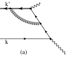
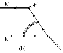
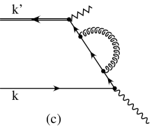
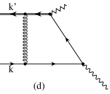
FIG. 2.: One-loop corrections to the radiative leptonic decay $B^{+}\to W\gamma$. The curly line represents a gluon. The quark wave function renormalization corrections are not shown.

FIG. 3.: Typical leading twist form factors $f_{i}(E_{\gamma})$ $(i=V,A)$ for $B\to\gamma e\nu$ decays. The continuous line shows the tree-level result, the dotted line includes one-loop corrections to the hard scattering amplitude, and the dashed line includes the resummed Sudakov form factor truncated with a cut-off at $(k_{+})_{min}=\Lambda_{QCD}$. We use $\alpha_{s}(m_{b})=0.3$ and $a=0.36$ GeV, $\omega=0.2$ GeV, corresponding to $\bar{\Lambda}=0.35$ GeV.

FIG. 4.: The photon spectrum in $B^{+}\to\gamma e^{+}\nu$ normalized to the pure muonic leptonic decay rate. The continuous line represents the tree-level result, assuming $R=3$ GeV^-1. The dotted line includes the effects of the one-loop strong correction (only the logarithms) with $\alpha_{s}(m_{b})=0.3$, and the dashed line includes the resummed Sudakov logs. The same parameters are used for the light-cone $B$ wave function as in Fig. 3.