On the choice of heavy baryon currents in the relativistic three-quark model

Abstract

We test the sensitivity of bottom baryon observables with regard to the choice of the interpolating three-quark currents within the relativistic three-quark model. We have found that the semileptonic decay rates are clearly affected by the choice of currents, whereas the asymmetry parameters show only a very weak dependence on the choice of current.

I Introduction

The forthcoming experimental data on exclusive bottom baryon decays call for a comprehensive theoretical analysis of their spectra and their decay properties. During the last decade heavy baryon transitions have been studied in detail within the Heavy Quark Effective Theory employing QCD sum rule methods or nonrelativistic and relativistic quark models, etc. (see, for example, the reviews in [1, 2] and the papers [3, 4, 5, 6, 7, 8, 9, 10, 11, 12, 13, 14, 15, 16, 17, 18, 19, 20, 21, 22, 23, 24, 25, 26, 27, 28]). The mass spectrum of heavy baryons as well as their exclusive and inclusive decays have been described successfully in these approaches incorporating the ideas of QCD. Preliminary results for the $\Lambda_{b}\to\Lambda_{c}$ baryon Isgur-Wise function and its slope have recently been obtained in Lattice QCD [29].

In the papers [14, 15, 16, 18, 30, 31, 32, 33] we proposed and developed a QCD motivated relativistic three-quark model (RTQM), which can be viewed as an effective quantum field approach based on an interaction Lagrangian of light and heavy baryons interacting with their constituent quarks. The coupling strengths of the baryons interacting with the three constituent quarks are determined by the compositeness condition $Z_{H}=0$ [31, 34] where $Z_{H}$ is the wave function renormalization constant of the hadron. The compositeness condition enables one to unambiguously and consistently relate the theories with both quark and hadron degrees of freedom to the effective Lagrangian approaches formulated in terms of hadron variables only (as, for example, Chiral Perturbation Theory [35] and its covariant extension to the baryon sector [36]). Our strategy is as follows. We start with an effective interaction Lagrangians written down in terms of quark and hadron variables. Then, by using Feynman rules, the $S$-matrix elements describing hadron-hadron interactions are given in terms of a set of quark Feynman diagrams. The compositeness condition serves to avoid double counting of quark and hadron degrees of freedom. The RTQM contains only a few model parameters: the masses of the light and heavy quarks, and certain scale parameters that are related to the size of the distribution of the constituent quarks inside the hadron. The RTQM has been previously used to compute the exclusive semileptonic, nonleptonic, strong and electromagnetic decays of charm and bottom baryons in the heavy quark limit $m_{Q}\to\infty$ always employing the same set of model parameters [14, 15, 16].

The objective of this paper is to continue the analysis of heavy baryon transitions within the RTQM [14, 15, 16, 17, 18, 30, 31, 32, 33]. In particular we shall investigate the dependence of heavy baryon observables calculated in the RTQM on the choice of three-quark baryon currents. In the heavy quark limit there remains a twofold ambiguity in the choice of interpolating currents for the ground state baryons. The properties of heavy baryons calculated in any model will in general depend on the choice taken for the baryon currents. It is therefore worthwhile to use a particular model and provide a detailed investigation of how the choice of interpolating currents affects the outcome of a dynamical calculation. For definiteness we shall limit our investigation to $b\to c$ semileptonic transitions of $\Lambda$-type and $\Omega$-type heavy baryons (such as $\Lambda_{b}\to\Lambda_{c}e\nu_{e}$, $\Sigma_{b}\to\Sigma_{c}e\nu_{e}$, etc.).

We proceed as follows. First we briefly explain the basic ideas of the RTQM. Next we obtain analytic expressions for the heavy baryon Isgur-Wise functions and calculate rates and differential distributions in baryonic $b\to c$ semileptonic transitions of ground state $\Lambda$-type and $\Omega$-type heavy baryons. We compare our numerical results with the results of other theoretical approaches.

II Relativistic Three-Quark Model

We start with a brief description of our approach called the Relativistic Three-Quark Model (RTQM). A detailed description of the RTQM can be found in Refs. [14, 16, 32, 33]. In the RTQM baryons are described as bound states of consitituent quarks. We denote the heavy baryons by $B_{Q}=Qq_{1}q_{2}$ which specifies a bound state of an infinitely large heavy quark $Q=b$ or $c$ and two light quarks $q_{1}$ and $q_{2}$ with masses $m_{q_{1}}$ and $m_{q_{2}}$. We express the spatial four-coordinates $(y_{i})$ of the constituent quarks in terms of the center-of-mass coordinate $(x)$ and the relative Jacobi coordinates (see ref. [14]):

$$y_{Q} = x\,,$$

$$y_{q_{1}} = x+3\xi_{1}-\sqrt{3}\xi_{2}\,,$$

$$y_{q_{2}} = x+3\xi_{1}+\sqrt{3}\xi_{2}\,.$$

The Lagrangian describing the interaction of a heavy baryon $B_{Q}$ with a single heavy quark $Q$ and two light quarks $q_{1}$ and $q_{2}$ simplifies in the heavy quark limit. The Lagrangian can be written as [14]

$${\cal L}_{B_{Q}}(x)=g_{B_{Q}}\bar{B}_{Q}(x)J_{B_{Q}}(x)+{\rm h.c.}$$ (1)

where $J_{B_{Q}}$ is a three-quark current with the quantum numbers of the heavy baryon given by

$$J_{B_{Q}}(x) = \Gamma_{1}Q^{a_{1}}(x)\!\int\!d^{4}\xi_{1}\!\int\!d^{4}\xi_{2}\,F_{B_{Q}}(\xi^{2}_{1}+\xi^{2}_{2})$$ (2)

$$\times q^{a_{2}}_{1}\!\left(x+3\xi_{1}-\sqrt{3}\xi_{2}\right)C\Gamma_{2}\lambda_{B_{Q}}$$ (3)

$$\times q^{a_{3}}_{2}\!\left(x+3\xi_{1}+\sqrt{3}\xi_{2}\right)\varepsilon^{a_{1}a_{2}a_{3}}\,,$$ (4)

$$F_{B_{Q}}(\xi^{2}_{1}+\xi^{2})=$$ (5)

$$\int\!\frac{d^{4}k_{1}}{(2\pi)^{4}}\!\int\!\frac{d^{4}k_{2}}{(2\pi)^{4}}e^{-ik_{1}\xi_{1}-ik_{2}\xi_{2}}{\widetilde{F}}_{B_{Q}}\!\left(\frac{k^{2}_{1}+k^{2}_{2}}{\Lambda^{2}_{B_{Q}}}\right).$$ (6)

Here $\Gamma_{1}$ and $\Gamma_{2}$ are appropriate strings of Dirac matrices, $\lambda_{B_{Q}}$ is a flavor matrix and $C=\gamma^{0}\gamma^{2}$ is the charge conjugation matrix. $F_{B_{Q}}$ is the heavy baryon vertex form factor defining the momentum distribution of light quarks within the heavy baryon.

Unlike the heavy meson case the heavy baryon Lagrangian (1) contains a twofold ambiguity in the choice of the spin-flavour structure of the heavy baryon currents $J_{B_{Q}}$ (even in the absence of derivative couplings). For the $\Lambda$-type baryons ($\Lambda_{Q}$, $\Xi_{Q}$) with a light spin zero diquark system one has a pseudoscalar current $J^{P}_{B_{Q}}$ and an axial current $J^{A}_{B_{Q}}$, both of which have the correct quantum numbers to serve as interpolating fields for the $\Lambda$-type baryons. Similarly for the $\Omega$-type baryons $\Omega_{Q}$, $\Sigma_{Q}$ and $\Omega^{\,*}_{Q}$, $\Sigma^{\,*}_{Q}$ with a spin one diquark system one has a a vector current $J^{V}_{B_{Q}}$ and a tensor current $J^{T}_{B_{Q}}$. In terms of the spinor and flavour structure the two respective currents in each case are given by [10, 13, 14, 37]

$$J^{P}_{\Lambda_{Q}} = \varepsilon^{abc}Q^{a}u^{b}C\gamma^{5}d^{c}$$ (7)

$$J^{A}_{\Lambda_{Q}} = \varepsilon^{abc}\gamma_{\mu}Q^{a}u^{b}C\gamma^{5}\gamma^{\mu}d^{c}$$ (8)

$$J^{V}_{\Omega_{Q}} = \varepsilon^{a}bc\gamma_{\mu}\gamma^{5}Q^{a}s^{b}C\gamma^{\mu}s^{c}$$ (10)

$$J^{T}_{\Omega_{Q}} = \varepsilon^{abc}\sigma_{\mu\nu}\gamma^{5}Q^{a}s^{b}C\sigma^{\mu\nu}s^{c}$$ (11)

$$J^{V;\mu}_{\Omega^{*}_{Q}} = \varepsilon^{abc}Q^{a}s^{b}C\gamma^{\mu}s^{c}$$ (13)

$$J^{T;\mu}_{\Omega^{*}_{Q}} = -i\varepsilon^{abc}\gamma_{\nu}Q^{a}s^{b}C\sigma^{\mu\nu}s^{c}$$ (14)

In this paper we investigate the sensitivity of observables on the choice of heavy baryon currents. We will consider general linear combinations of the two possible currents for the ground states of heavy baryons. Thus we write

$$J_{\Lambda_{Q}}\bigl{(}x\bigr{)} = \alpha_{P}J^{P}_{\Lambda_{Q}}\bigl{(}x\bigr{)}+\alpha_{A}J^{A}_{\Lambda_{Q}}\bigl{(}x\bigr{)}$$ (15)

$$J_{\Omega_{Q}}\bigl{(}x\bigr{)} = \beta_{V}J^{V}_{\Omega_{Q}}\bigl{(}x\bigr{)}+\beta_{T}J^{T}_{\Omega_{Q}}\bigl{(}x\bigr{)}$$ (16)

$$J^{\mu}_{\Omega^{*}_{Q}}\bigl{(}x\bigr{)} = \beta_{V}J^{V;\mu}_{\Omega^{*}_{Q}}\bigl{(}x\bigr{)}+\beta_{T}J^{T;\mu}_{\Omega^{*}_{Q}}\bigl{(}x\bigr{)}$$ (17)

Since the $\Omega_{Q}$ and the $\Omega_{Q}^{*}$ are members of the same heavy quark symmetry doublet the coefficients $\beta_{V}$ and $\beta_{T}$ are the same for both. As a result of the twofold ambiguity we have to introduce the two additional parameters $R_{\Lambda}=\alpha_{A}/\alpha_{P}$ and $R_{\Omega}=\beta_{T}/\beta_{V}$.

Next we specify our model parameters. The heavy-baryon quark coupling constants $g_{B_{Q}}$ are determined by the compositeness condition [6, 16, 31, 34]. The compositeness condition implies that the renormalization constant of the hadron wave function is set equal to zero: $Z_{B_{Q}}=1-g_{B_{Q}}^{2}\Sigma^{\prime}_{B_{Q}}(M_{B_{Q}})=0$ where $\Sigma^{\prime}_{B_{Q}}$ is the derivative of the baryon mass operator and $M_{B_{Q}}$ is the heavy baryon mass. In Eq. (2) we have introduced a baryon-three-quark vertex form factor written as $\tilde{F}_{B_{Q}}((k_{1}^{2}+k_{2}^{2})/\Lambda_{B_{Q}}^{2})$ where $\Lambda_{B_{Q}}$ is a scale parameter defining the distribution of the light quarks in the heavy baryon. Any choice of vertex function $F_{B_{Q}}$ is appropriate as long as it falls off sufficiently fast in the ultraviolet region to render the Feynman diagrams ultraviolet finite. In principle, its functional form would be calculable from the solutions of the Bethe-Salpeter equations for the baryon bound states [17] which is, however, an untractable problem at present. In our previous analysis [32] we found that, using various forms for the vertex function, the hadron observables are insensitive to the details of the functional form of the hadron-quark vertex form factor. We will use this observation as a guiding principle and choose a simple Gaussian forms for the vertex function $F_{B_{Q}}$. Its Fourier transform reads [14, 15, 16, 33]

$$\tilde{F}_{B_{Q}}\left(\frac{k^{2}_{1}+k^{2}_{2}}{\Lambda^{2}_{B_{Q}}}\right)=\exp\left(\frac{k_{1}^{2}+k_{2}^{2}}{\Lambda_{B_{Q}}^{2}}\right)$$ (18)

where $\Lambda_{B_{Q}}$ is a scale parameter defining the distribution of $u$ and $d$ quarks in the heavy baryon. For the light quark propagator with a constituent mass $m_{q}$ we shall use the standard form of the free fermion propagator

$$S_{q}(k)=\frac{1}{m_{q}-\not\!k}$$ (19)

where $m_{q}=m$ for the $u$ or $d$ quarks (we work in the isospin symmetry limit) and $m_{q}=m_{s}$ for the strange quark. For the heavy quark propagator we shall use the leading term $S_{v}(k,\bar{\Lambda}_{q_{1}q_{2}})$ in the inverse mass expansion of the free fermion propagator:

$$S_{Q}(p+k) = \frac{1}{m_{Q}-(\not\!p+\not\!k)}\,,$$ (20)

$$= S_{v}(k,\bar{\Lambda}_{q_{1}q_{2}})+O\left(\frac{1}{m_{Q}}\right)$$ (21)

$$S_{v}(k,\bar{\Lambda}_{q_{1}q_{2}}) = -\frac{(1+\not\!v)}{2(v\cdot k+\bar{\Lambda}_{q_{1}q_{2}})}$$ (22)

We introduce the mass difference parameter $\displaystyle{\bar{\Lambda}_{q_{1}q_{2}}=M_{Qq_{1}q_{2}}-m_{Q}}$ which is the difference between the heavy baryon mass $M_{Qq_{1}q_{2}}\equiv M_{B_{Q}}$ and the heavy quark mass $m_{Q}$. The four-velocity of the heavy quark is denoted by $v$ as usual. As in the light quark propagator we shall neglect a possible mass difference between the constituent $u$- and $d$-quark. Thus there are altogether three independent mass parameters: $\bar{\Lambda}$ for heavy baryons without strange quarks, $\bar{\Lambda}_{s}$ for heavy baryons with a single strange quark and $\bar{\Lambda}_{ss}$ for doubly strange heavy baryons.

Our set of model parameters are the following: the masses of the light quarks $m$ and $m_{s}$, the vertex scale parameter $\Lambda_{B_{Q}}$, parameters related to the heavy quark propagator $\bar{\Lambda}$, $\bar{\Lambda}_{s}$ and $\bar{\Lambda}_{ss}$ and the two parameters $R_{\Lambda}=\alpha_{A}/\alpha_{P}$ and $R_{\Omega}=\beta_{T}/\beta_{V}$ related to the twofold ambiguity in the choice of the heavy baryon currents for the $\Lambda$-type and $\Omega$-type baryons. The parameter $m=420$ MeV has been fixed in Ref [33] from an analysis of nucleon data. The parameters $\Lambda_{B_{Q}}$, $m_{s}$ and $\bar{\Lambda}$ are taken from an analysis of the $\Lambda_{c}^{+}\to\Lambda^{0}+e^{+}+\nu_{e}$ decay data. A good description of the present average value of the branching ratio $B(\Lambda_{c}^{+}\to\Lambda e^{+}\nu_{e})=2.2\%$ can be achieved with $\Lambda_{B_{Q}}=1.8$ GeV, $m_{s}=570$ MeV and $\bar{\Lambda}=600$ MeV [18]. In addition, the value of the strange quark mass $m_{s}=570$ MeV gives the best description of the magnetic moments of light hyperons ($\Lambda$, $\Sigma$, $\Xi$). The values of the parameters $\bar{\Lambda}_{s}$ and $\bar{\Lambda}_{ss}$ are determined from the heuristic relations $\bar{\Lambda}_{s}=\bar{\Lambda}+(m_{s}-m)$ and $\bar{\Lambda}_{ss}=\bar{\Lambda}+2(m_{s}-m)$, which gives $\bar{\Lambda}_{s}=750$ MeV and $\bar{\Lambda}_{ss}=900$ MeV. Finally, the mass values of the charm and bottom baryon states are taken from Ref. [17] (masses of $\Lambda_{Q}$, $\Xi_{c}$, $\Sigma_{c}$ and $\Sigma^{*}_{c}$ baryons) and Ref. [14] (masses of $\Xi_{b}$, $\Sigma_{b}$, $\Sigma^{*}_{b}$ and $\Omega_{Q}$ baryons).

III Results

A Matrix elements of semileptonic transitions of heavy baryons

The semileptonic $b\to c$ transitions of heavy baryons are described by the triangle two-loop quark diagram Fig. 1.

FIG. 1.: Feynman diagram describing the semileptonic $b\to c$ decay of heavy baryons $B_{b}\to B_{c}+e+\nu_{e}$

It takes the following form in the heavy quark limit

$$\bar{u}(v^{\prime})M^{\mu}(v,v^{\prime})u(v)=$$ (26)

$$\frac{G_{F}}{\sqrt{2}}V_{cb}g^{i}_{B_{Q}}g^{f}_{B_{Q}}\bar{u}(v^{\prime})\Gamma^{f}_{1}\!(1+\not\!v^{\prime})O^{\mu}(1+\not\!v)\Gamma^{i}_{1}u(v)\cdot I^{if}_{q_{1}q_{2}}$$

$$I^{if}_{q_{1}q_{2}}(v,v^{\prime})=\int\!\frac{d^{4}k_{1}}{2\pi^{2}i}\!\int\!\frac{d^{4}k_{2}}{2\pi^{2}i}{\widetilde{F}}^{2}_{B_{Q}}\!\left(\frac{9k^{2}_{1}+3k^{2}_{2}}{\Lambda_{B_{Q}}}\right)$$

$$\times \frac{{\rm tr}[\Gamma^{f}_{2}S_{q_{2}}(k_{2})\Gamma^{i}_{2}S_{q_{1}}(k_{1}+k_{2})]}{\left[k_{1}v+\bar{\Lambda}_{q_{1}q_{2}}\right]\left[k_{2}v^{\prime}+\bar{\Lambda}_{q_{1}q_{2}}\right]}$$ (27)

where $G_{F}$ is the Fermi weak effective coupling, $V_{cb}=0.04$ is the CKM matrix element, $g_{B_{Q}}^{i}$ and $g_{B_{Q}}^{f}$ are the couplings constants of quarks with the initial (i) and the final (f) baryon, respectively.

The calculational techniques of how to deal with the integral (26) can be found in Refs. [16, 18]. All dimensional parameters in the Feynman loop integrals are expressed in units of $\Lambda_{B_{Q}}$. The Feynman integrals are calculated in the Euclidean region both for internal and external momenta. The final results are obtained by analytic continuation of the external momenta to the physical region after the internal momenta have been integrated out.

After a few steps of calculation of the overlap integral $\displaystyle{I^{if}_{q_{1}q_{2}}}$ can be written as

$$I^{if}_{q_{1}q_{2}}(v,v^{\prime}) = \int\limits^{\infty}_{0}\!d^{\,4}\alpha\frac{{\widetilde{F}}^{2}_{B_{Q}}(6z)}{4{\left|A\right|}^{2}}$$ (28)

$$\times \left\{m_{q_{1}}m_{q_{2}}{\rm tr}\Bigl{[}\Gamma^{i}_{2}\Gamma^{f}_{2}\Bigr{]}\right.$$ (29)

$$- \left.m_{q_{1}}\frac{A^{-1}_{11}+A^{-1}_{12}}{2}{\rm tr}\Bigl{[}\Gamma^{i}_{2}\bigl{(}\not\!v\alpha_{3}+{\not\!v}^{\,\prime}\alpha_{4}\bigr{)}\Gamma^{f}_{2}\Bigr{]}\right.$$ (30)

$$- m_{q_{2}}\frac{A^{-1}_{12}}{2}{\rm tr}\Bigl{[}\Gamma^{i}_{2}\Gamma^{f}_{2}\bigl{(}\not\!v\alpha_{3}+{\not\!v}^{\,\prime}\alpha_{4}\bigr{)}\Bigr{]}$$ (31)

$$+ \frac{A^{-1}_{12}\Bigl{(}A^{-1}_{11}+A^{-1}_{12}\Bigr{)}}{4}{\rm tr}\Bigl{[}\Gamma^{i}_{2}\bigl{(}\not\!v\alpha_{3}+{\not\!v}^{\,\prime}\alpha_{4}\bigr{)}$$ (32)

$$\times \Gamma^{f}_{2}\bigl{(}\not\!v\alpha_{3}+{\not\!v}^{\,\prime}\alpha_{4}\bigr{)}\Bigr{]}$$ (33)

$$- \frac{A^{-1}_{12}+A^{-1}_{22}}{4}{\rm tr}\Bigl{[}\Gamma^{i}_{2}\gamma^{\alpha}\Gamma^{f}_{2}\gamma_{\alpha}\Bigr{]}$$ (34)

$$\times \left.\left(\alpha_{3}\frac{dz}{d\alpha_{3}}+\alpha_{4}\frac{dz}{d\alpha_{4}}\right)\right\}$$ (35)

where

$$z = m^{2}_{q_{1}}\alpha_{1}+m^{2}_{q_{2}}\alpha_{2}-\bar{\Lambda}_{q_{1}q_{2}}\bigl{(}\alpha_{3}+\alpha_{4}\bigr{)}$$ (36)

$$+ \frac{2+\alpha_{1}+\alpha_{2}}{4\left|A\right|}\Bigl{[}\alpha^{2}_{3}+\alpha^{2}_{4}+2\alpha_{3}\alpha_{4}\omega\Bigr{]}$$ (37)

$$A=\left(\begin{array}[]{ll}2+\alpha_{2}&1+\alpha_{2}\\[8.53581pt] 1+\alpha_{2}&2+\alpha_{1}+\alpha_{2}\end{array}\right)$$ (40)

Here $|A|={\rm det}\{A\}$.

In the heavy quark limit the matrix elements describing semileptonic $b\to c$ transitions can be expressed through the three universal Isgur-Wise functions $\zeta(\omega)$, $\xi_{1}(\omega)$ and $\xi_{2}(\omega)$ of the dimensionless variable $\omega=v\cdot v^{\prime}$ where $v$ and $v^{\prime}$ are the four-velocities of initial and final baryons, respectively. One finds

$\Lambda_{\,b}\longrightarrow\Lambda_{\,c}$ transition

$$\left<\Lambda_{\,c}\bigl{(}v^{\,\prime}\bigr{)}\!\left|\,\overline{b}\,\Gamma\,c\,\right|\!\Lambda_{\,b}\bigl{(}v\bigr{)}\right>=\zeta\bigl{(}\omega\bigr{)}\overline{u}\bigl{(}v^{\,\prime}\bigr{)}\Gamma u\bigl{(}v\bigr{)},$$ (41)

$\Omega_{b}\rightarrow\Omega_{c}(\Omega_{c}^{*})$ transition

$$\left<\Omega_{c}\bigl{(}v^{\,\prime}\bigr{)}\,\mbox{or}\,\Omega_{c}^{\,*}\bigl{(}v^{\,\prime}\bigr{)}\!\left|\,\overline{b}\,\Gamma\,c\,\right|\!\Lambda_{\,b}\bigl{(}v\bigr{)}\right>=$$ (42)

$${\overline{B}}^{\mu}_{\,c}\bigl{(}v^{\,\prime}\bigr{)}\Gamma B^{\,\nu}_{\,b}\bigl{(}v\bigr{)}\bigl{[}-\xi_{1}\bigl{(}\omega\bigr{)}g_{\mu\nu}+\xi_{2}\bigl{(}\omega\bigr{)}v_{\mu}v^{\,\prime}_{\nu}\bigr{]}$$ (43)

where the spinor tensor $\displaystyle{B^{\,\nu}_{b}(v)}$ obeys the Rarita-Schwinger constraints $\displaystyle{v_{\nu}B^{\,\nu}_{b}(v)=0}$ and $\gamma_{\nu}B^{\,\nu}_{b}(v)=0$. The spin-wave functions are written as following:

$$\begin{array}[]{llll}B^{\,\mu}_{Q}(v)&=&\displaystyle{\frac{\gamma^{\,\mu}+v^{\,\mu}}{\sqrt{3}}}\gamma^{\,5}u_{\,\Omega_{Q}}(v)\hfill&\mbox{for $\Omega_{Q}$ states}\\[8.53581pt] B^{\,\mu}_{Q}(v)&=&u^{\,\mu}_{\,\Omega^{\,*}_{Q}}(v)\hfill&\mbox{for $\Omega^{\,*}_{Q}$ states}\end{array}$$ (44)

where the $u_{\,\Omega_{Q}}\bigl{(}v\bigr{)}$ and $u^{\,\mu}_{\,\Omega^{\,*}_{Q}}\bigl{(}v\bigr{)}$ are the spin-$\displaystyle{1\!\left/2\right.}$ spinor and the Rarita-Schwinger spinor, respectively.

B Baryonic Isgur-Wise functions

A direct evaluation of the baryon Isgur-Wise functions with the currents (15) gives the following analytical results:

$$\zeta\bigl{(}\omega\bigr{)}=\frac{F_{0}\bigl{(}\omega\bigr{)}}{F_{0}\bigl{(}1\bigr{)}}\,,\hskip 5.69046pt\xi_{1}\bigl{(}\omega\bigr{)}=\frac{F_{1}\bigl{(}\omega\bigr{)}}{F_{1}\bigl{(}1\bigr{)}}\,,\hskip 5.69046pt\xi_{2}\bigl{(}\omega\bigr{)}=\frac{F_{2}\bigl{(}\omega\bigr{)}}{F_{1}\bigl{(}1\bigr{)}}$$ (45)

$$F_{\rm I}(\omega)=\displaystyle{\int\limits_{0}^{\infty}\!dx\,x\!\int\limits_{0}^{\infty}}\!\displaystyle{dy\,y\int\limits_{0}^{1}\!d\phi\!\int\limits_{0}^{1}\!d\theta\,\frac{R_{I}\bigl{(}\omega\bigr{)}}{|A|^{2}}{\widetilde{F}}^{2}_{B_{Q}}\bigl{(}6z\bigr{)}}$$ (46)

where

$$R_{0}(\omega) = m_{q_{1}}m_{q_{2}}(\alpha^{2}_{P}+\alpha^{2}_{A}\,\omega)$$ (47)

$$+ \left(2\alpha^{2}_{P}-\alpha^{2}_{A}\,\omega\right)\frac{x}{\left|A\right|}$$ (48)

$$\times \left[\frac{2+y}{\left|A\right|}x\Bigl{(}1+2\phi(1-\phi)(\omega-1)\Bigr{)}-2\bar{\Lambda}_{q_{1}q_{2}}\right]$$ (49)

$$+ (\omega+1)[m_{q_{1}}(1+y\theta)$$ (50)

$$+ m_{q_{2}}(1+y(1-\theta))]\alpha_{P}\alpha_{A}\frac{x}{\left|A\right|}\,$$ (51)

$$+ \frac{x^{2}}{4\,|A|^{2}}\Bigl{[}\alpha^{2}_{P}+\alpha^{2}_{A}\,\omega$$ (52)

$$+ 2\phi\bigl{(}1-\phi\bigr{)}\bigl{(}\omega-1\bigr{)}\bigl{(}\alpha^{2}_{P}-\alpha^{2}_{A}\bigr{)}\Bigr{]}$$ (53)

$$\times \Bigl{[}1+y+y^{2}\theta(1-\theta)\Bigr{]},$$ (54)

$$R_{1}(\omega) = m_{q_{1}}m_{q_{2}}(\beta^{2}_{V}+\beta^{2}_{T}\,\omega)$$ (56)

$$+ \beta^{2}_{V}\frac{x}{\left|A\right|}\left[\frac{2+y}{\left|A\right|}x\Bigl{(}1+2\phi(1-\phi)(\omega-1)\Bigr{)}-2{\bar{\Lambda}}_{q_{1}q_{2}}\right]$$ (57)

$$+ (\omega+1)[m_{q_{1}}(1+y\theta)$$ (58)

$$+ m_{q_{2}}(1+y(1-\theta))]\,\beta_{V}\beta_{T}\frac{x}{\left|A\right|}\,$$ (59)

$$+ \frac{x^{2}}{4\,|A|^{2}}\Bigl{[}\beta^{2}_{V}+\beta^{2}_{T}\,\omega$$ (60)

$$+ 2\phi(1-\phi)(\omega-1)(\beta^{2}_{V}-\beta^{2}_{T})\Bigr{]}$$ (61)

$$\times \Bigl{[}1+y+y^{2}\theta(1-\theta)\Bigr{]},$$ (62)

$$R_{2}(\omega) = m_{q_{1}}m_{q_{2}}\,\beta^{2}_{T}+[m_{q_{1}}(1+y\theta)$$ (64)

$$+ m_{q_{2}}(1+y(1-\theta))]\,\beta_{V}\beta_{T}\frac{x}{\left|A\right|}\,$$ (65)

$$+ \frac{x^{2}}{4\,|A|^{2}}\Bigl{[}\beta^{2}_{T}+2\phi(1-\phi)(\beta^{2}_{V}-\beta^{2}_{T})\Bigr{]}$$ (66)

$$\times \Bigl{[}1+y+y^{2}\theta(1-\theta)\Bigr{]}\,.$$ (67)

Here

$$\left|A\right|=3+2y+y^{\,2}\theta\bigl{(}1-\theta\bigr{)}\,$$ (69)

$$z=y(m_{q_{1}}^{2}\theta+m_{q_{2}}^{2}(1-\theta))\,$$

$$+ x\left[\frac{2+y}{4\left|A\right|}x\Bigl{(}1+2\phi\bigl{(}1-\phi\bigr{)}\bigl{(}\omega-1\bigr{)}\Bigr{)}-\bar{\Lambda}_{q_{1}q_{2}}\right]\,.$$ (70)

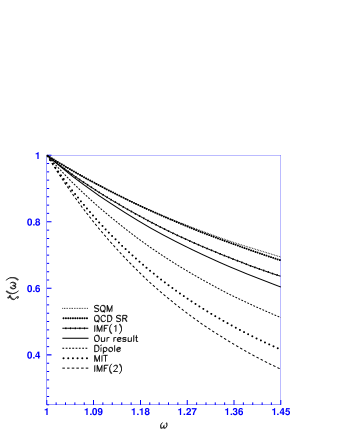
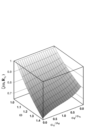
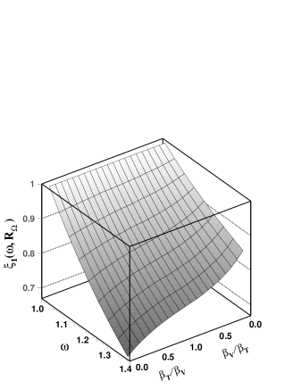
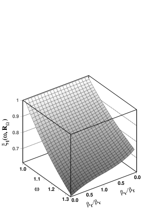
In Fig. 2 we depict our model predictions for the $\omega$-dependence of the form factor $\zeta(\omega)$. We compare our prediction for $\zeta(\omega)$ with results from the simple quark model [22], QCD sum rules [21], the infinite momentum frame quark model [23, 24], the dipole model [23] and the MIT bag model [25]. In Fig. (3-5) we exhibit the sensitivity of the Isgur-Wise functions $\zeta(\omega)$ and $\xi_{1}(\omega)$ to the choice of the three-quark currents with the quantum numbers of $\Lambda$-type and $\Omega$-type baryons. We have kept the values of the other model parameters fixed in this comparison ($\bar{\Lambda}$=0.6 GeV, $\bar{\Lambda}_{\{ss\}}$=0.9 GeV, and $\Lambda_{B_{Q}}$=1.8 GeV). The Isgur-Wise function $\zeta(\omega)$ for the $\Lambda_{b}\to\Lambda_{c}$ transition calculated with the pseudoscalar current can be seen to lie below the one calculated with the axial current. This will result in different rate predictions. Similarly, in the case of the $\Omega$-type baryons (see, Fig. 4 and Fig. 5), the vector current Isgur-Wise function lies below the tensor current Isgur-Wise function.

The radii of the form factors $\displaystyle{\zeta}$ and $\displaystyle{\xi_{1}}$ (or the slope parameters) are defined by

$$F(\omega)=1-\rho^{\,2}_{F}(\omega-1)+\ldots$$ (71)

where $F=\zeta$ or $\xi_{1}$. Varying the parameters $R_{\Lambda}$ and $R_{\Omega}$ in the range $[0,\infty)$ and keeping the values of $\Lambda_{B_{Q}}$ and $\bar{\Lambda}_{q_{1}q_{2}}$ fixed, the slopes of the $\Lambda_{b}$ and $\Sigma_{b}$ baryon Isgur-Wise functions are given by $\rho^{2}_{\zeta}=1.05\pm 0.30$ and $\rho^{2}_{\xi_{1}}=1.07\pm 0.30$. In particular, one has

$$\begin{array}[]{ll}\rho^{2}_{\zeta}=1.35&\hfill\mbox{ for \, $\alpha_{A}/\alpha_{P}=0$ }\,,\\[2.84526pt] \rho^{2}_{\zeta}=1.05&\hfill\mbox{ for \, $\alpha_{P}/\alpha_{A}=1$ }\,,\\[2.84526pt] \rho^{2}_{\zeta}=0.75&\hfill\mbox{ for \, $\alpha_{P}/\alpha_{A}=0$ }\,,\\[2.84526pt] \rho_{\xi_{1}}=1.37&\hfill\mbox{ for \, $\beta_{T}/\beta_{V}=0$ }\,,\\[2.84526pt] \rho^{2}_{\xi_{1}}=1.06&\hfill\mbox{ for \, $\beta_{T}/\beta_{V}=1$ }\,,\\[2.84526pt] \rho^{2}_{\xi_{1}}=0.75&\hfill\mbox{ for \, $\beta_{V}/\beta_{T}=0$ }\,.\end{array}$$ (78)

Finally we cite the values of the charge radius of the $\Lambda_{b}\to\Lambda_{c}$ Isgur-Wise function of other theoretical model calculations. They vary in a rather large range:

$$\rho^{2}_{\zeta}:$$

$$\begin{array}[]{ccccccc}$\cite[cite]{[\@@bibref{Number}{IMF1}{}{}]}$&$ \cite[cite]{[\@@bibref{Number}{Skyrme}{}{}]} $&$ \cite[cite]{[\@@bibref{Number}{Dai}{}{}]} $&$\cite[cite]{[\@@bibref{Number}{SQM}{}{}]}$&$\cite[cite]{[\@@bibref{Number}{Sadzik_Zalew}{}{}]}$&$\cite[cite]{[\@@bibref{Number}{Grozin}{}{}]}$&$\cite[cite]{[\@@bibref{Number}{Bowler}{}{}]}$\\ \hline\cr$\ 1.44 \ $&$ \ 1.3\ $&$ \ 0.65 \ $&$\ 1.01 \ $&$ \ 2.35 \ $&$ \ 1.15 \ $&$\ $1.2^{+0.8}_{-1.1}$\ $\\ \end{array}$$ (81)

C Rates, distributions and asymmetry parameters

In this section we present our numerical results on rates, distributions and asymmetry parameters for the $b\to c$ flavour changing heavy baryon decays. The standard expressions for observables of semileptonic decays of bottom baryons (decay rates, differential distributions, leptonic spectra, and asymmetry parameters) have simple forms when expressed in terms of helicity amplitudes. The set of HQL helicity amplitudes describing transitions of bottom baryons into charm baryons can be found in Ref. [14]. In Table I we present our numerical results for the total and partial rates of $\Lambda_{b}\to\Lambda_{c}e\nu_{e}$ transitions using three particular choices of the $R_{\Lambda}$ parameter: $\alpha_{A}/\alpha_{P}=0$, $\alpha_{P}/\alpha_{A}=0$ and $\alpha_{P}/\alpha_{A}=1$. One can see that the pseudoscalar current consistently gives smaller rate values. However, the numbers show that the difference between the three choices is not very significant. Our results are in good agreement with the experimental upper limit for the rate $\Gamma(\Lambda_{b}\to\Lambda_{c}e\nu_{e})$ given by $(6.67\pm 2.73)\times 10^{-10}$ s ^-1. For comparison we present the results of some other theoretical approaches. In Table II we give our predictions for the other semileptonic decay rates of bottom baryons.

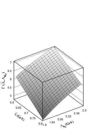
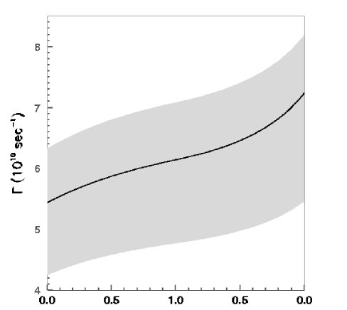
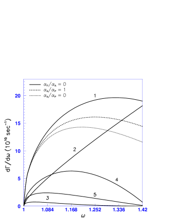
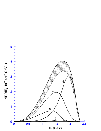
In Fig. 6 we depict the dependence of the $\Lambda_{b}\to\Lambda_{c}e\nu_{e}$ rate on the parameters $\bar{\Lambda}$ and $\Lambda_{B_{Q}}$ where the latter parameters are varied in the regions 0.6 GeV $<\bar{\Lambda}<$ 0.8 GeV and 1.8 GeV $<\Lambda_{B_{Q}}<$ 2.5 GeV and the current mixing parameter $R_{\Lambda}$ equals to $R_{\Lambda}=1$. For the rate we find $\Gamma(\Lambda_{b}\to\Lambda_{c}e\nu_{e})=(5.9.\pm 1.1)\times 10^{10}$ s^-1 where the theoretical error results from the variation of the parameters $\bar{\Lambda}$ and $\Lambda_{B_{Q}}$ in the indicated range. In Fig. 7 we depict the dependence of the rate $\Gamma(\Lambda_{b}\to\Lambda_{c}e\nu_{e})$ on the current mixing parameter $R_{\Lambda}=\alpha_{A}/\alpha_{P}$ with the model parameters $\bar{\Lambda}$ and $\Lambda_{B_{Q}}$ being varied in the region $\displaystyle{0.6\mbox{ GeV}<\bar{\Lambda}<0.8\mbox{ GeV}}$ and $\displaystyle{1.8\mbox{ GeV}<\Lambda_{B_{Q}}<2.5\mbox{ GeV}}$. The solid curve corresponds to the set $\bar{\Lambda}=0.6$ GeV and $\Lambda_{B_{Q}}=1.8$ GeV. It it seen that the rate $\Gamma(\Lambda_{b}\to\Lambda_{c}e\nu_{e})$ changes in the interval $(6.2\pm 2)\times 10^{-10}$ s ^-1. Note the remarkable agreement of our predictions with the available upper experimental limit for the rate $\Gamma(\Lambda_{b}\to\Lambda_{c}e\nu_{e})=(6.67\pm 2.73)\times 10^{-10}$ s ^-1. In Fig. 8 and Fig. 9 we present our results for the differential decay distribution and the lepton spectra in the semileptonic decay $\Lambda_{b}\to\Lambda_{c}e\bar{\nu}_{e}$. Finally, in Table III we give our predictions for the asymmetry parameters (for their definitions, see [7]) which can be measured in the two cascade decays of the $\Lambda_{b}$ baryon. For comparison we also present the results of other theoretical approaches.

TABLE I.: Total and partial rates of the semileptonic decay $\Lambda_{b}^{0}\to\Lambda_{c}^{+}e^{-}\bar{\nu}_{e}$ (in $10^{10}~{}{\mbox{sec}}^{-1}$) for $\left|V_{bc}\right|=0.04$, $\Lambda_{B_{Q}}=1.8$ GeV, $\bar{\Lambda}=0.6$ GeV, $\bar{\Lambda}_{s}=0.75$ GeV, $\bar{\Lambda}_{ss}=0.9$ GeV.

Approach		$\Gamma$	$\Gamma_{T_{+}}$	$\Gamma_{T_{-}}$	$\Gamma_{L_{+}}$	$\Gamma_{L_{-}}$
	$\alpha_{A}/\alpha_{P}=0$	5.43	0.52	1.53	0.11	3.27
Our approach	$\alpha_{A}/\alpha_{P}=1$	6.15	0.57	1.69	0.12	3.77
	$\alpha_{P}/\alpha_{A}=0$	7.23	0.63	1.93	0.13	4.54
IMF [23]		4.28	0.41	1.20	0.09	2.58
IMF [24]		4.89	0.44	1.53	0.10	2.82
Dipole [23]		5.42	0.55	1.58	0.12	3.17
QCD Sum Rule [27]		6.16	0.43	1.86	0.10	3.77
Large $N_{c}$ [27]		5.51	0.34	1.45	0.09	2.63
Experiment [38]		$<$ 6.67$\pm$ 2.73

TABLE II.: Total and partial semileptonic rates of bottom baryons (in $10^{10}~{}{\mbox{sec}}^{-1}$) for $\left|V_{bc}\right|=0.04,$ $\Lambda_{B_{Q}}=1.8$ GeV, $\bar{\Lambda}=0.6$ GeV. $T$ and $L$ stand for the transverse and longitudinal components of the transition and $(\pm)$ denote the helicity of the daughter baryon.

Decay mode	Currents mixing	$\Gamma$	$\Gamma_{T_{+}}$	$\Gamma_{T_{-}}$	$\Gamma_{L_{+}}$	$\Gamma_{L_{-}}$
	$\alpha_{A}/\alpha_{P}=0$	5.98	0.59	1.64	0.13	3.62
$\Xi^{0}_{b}\to\Xi^{+}_{c}e^{-}\bar{\nu}_{e}$	$\alpha_{A}/\alpha_{P}=1$	6.67	0.63	1.80	0.13	4.11
	$\alpha_{P}/\alpha_{A}=0$	7.72	0.70	2.02	0.14	4.86
	$\beta_{A}/\beta_{P}=0$	2.10	0.08	0.24	1.39	0.39
$\Sigma^{+}_{b}\to\Sigma^{++}_{c}e^{-}\bar{\nu}_{e}$	$\beta_{A}/\beta_{P}=1$	2.23	0.07	0.21	1.65	0.30
	$\beta_{P}/\beta_{A}=0$	2.51	0.07	0.18	2.03	0.23
	$\beta_{A}/\beta_{P}=0$	1.60	0.07	0.19	1.07	0.27
$\Omega^{-}_{b}\to\Omega^{0}_{c}e^{-}\bar{\nu}_{e}$	$\beta_{A}/\beta_{P}=1$	1.68	0.07	0.17	1.23	0.21
	$\beta_{P}/\beta_{A}=0$	1.86	0.06	0.15	1.48	0.17
	$\beta_{A}/\beta_{P}=0$	3.69	0.50	1.27	0.86	1.06
$\Sigma^{+}_{b}\to\Sigma^{*++}_{c}e^{-}\bar{\nu}_{e}$	$\beta_{A}/\beta_{P}=1$	3.72	0.52	1.31	0.94	0.95
	$\beta_{P}/\beta_{A}=0$	3.84	0.54	1.39	1.05	0.86
	$\beta_{A}/\beta_{P}=0$	4.29	0.56	1.45	1.02	1.26
$\Omega^{-}_{b}\to\Omega^{*0}_{c}e^{-}\bar{\nu}_{e}$	$\beta_{A}/\beta_{P}=1$	4.33	0.58	1.50	1.12	1.13
	$\beta_{P}/\beta_{A}=0$	4.43	0.60	1.58	1.24	1.01

TABLE III.: Asymmetry parameters of semileptonic $\Lambda_{b}$ baryon decay for $\Lambda_{B_{Q}}=1.8$ GeV, $\bar{\Lambda}=0.6$ GeV.

Approach		$\alpha$	$\alpha^{\prime}$	$\alpha^{\prime\prime}$	$\gamma$	$\alpha_{P}$	$\gamma_{P}$
	$\alpha_{A}/\alpha_{P}=0$	-0.77	-0.11	-0.53	0.55	0.40	-0.16
Our approach	$\alpha_{A}/\alpha_{P}=1$	-0.78	-0.11	-0.55	0.54	0.41	-0.16
	$\alpha_{P}/\alpha_{A}=0$	-0.79	-0.11	-0.57	0.52	0.43	-0.15
IMF [23]		-0.76	-0.11	-0.53	0.55	0.39	-0.16
Dipole [23]		-0.75	-0.12	-0.51	0.57	0.37	-0.17
QCD Sum Rule [27]		-0.83	-0.14	-0.57	0.48	0.38	-0.17
Large $N_{c}$ [27]		-0.81	-0.15	-0.53	0.50	0.34	-0.19

FIG. 2.: The Isgur-Wise function $\zeta(\omega)$ of the decay $\Lambda^{0}_{b}\to\Lambda^{+}_{c}e^{-}\bar{\nu}_{e}$: SQM (Simple Quark Model, Ref. [22]); QCD SR (QCD Sum Rule, Ref. [21]); IMF(1) (Infinite Momentum Frame Quark Model, Ref. [23]); IMF(2) (Infinite Momentum Frame Quark Model, Ref. [24]); Our result (for $\bar{\Lambda}=0.6$ GeV; $\Lambda_{B_{Q}}=1.8$ GeV, $\alpha_{A}=0$); Dipole (Dipole form factor, Ref. [23]); MIT (MIT Bag Model, Ref. [25]).

FIG. 3.: The sensitivity of the Isgur-Wise function $\zeta(\omega)$ ($\Lambda_{b}$-decay) on the choice of the three-quark currents at fixed values of $\Lambda_{B_{Q}}$=1.8 GeV and $\bar{\Lambda}=0.6$ GeV.

FIG. 4.: The sensitivity of the Isgur-Wise function $\xi_{1}$ ($\Sigma_{b}$-decay) on the choice of three-quark currents at fixed values of $\Lambda_{B_{Q}}=1.8$ GeV and $\bar{\Lambda}=0.6$ GeV.

FIG. 5.: The sensitivity of the Isgur-Wise function $\xi_{1}$ ($\Omega_{b}$-decay) on the choice of three-quark currents at fixed values of $\Lambda_{B_{Q}}=1.8$ GeV and $\bar{\Lambda}_{ss}=0.9$ GeV.

FIG. 6.: Sensitivity of the total rate of $\Lambda_{b}\to\Lambda_{c}+e+\nu_{e}$ transition on the choice of the model parameters $\bar{\Lambda}$ and $\Lambda_{B_{Q}}$ keeping the parameter $R_{\Lambda}$ fixed at $R_{\Lambda}=1$.

FIG. 7.: The sensitivity of the $\Lambda_{b}\to\Lambda_{c}+e\nu_{e}$ decay rate on the choice of three-quark currents parametrized by the ratio $R_{\Lambda}=\alpha_{A}/\alpha_{P}$. The shaded region corresponds to the range of the total rate with the model parameters $\bar{\Lambda}$ and $\Lambda_{B_{Q}}$ being varied in the region $\displaystyle{0.6\mbox{ GeV}<\bar{\Lambda}<0.8\mbox{ GeV}}$ and $\displaystyle{1.8\mbox{ GeV}<\Lambda_{B_{Q}}<2.5\mbox{ GeV}}$. The solid heavy curve corresponds to the set $\bar{\Lambda}=0.6$ GeV and $\Lambda_{B_{Q}}=1.8$ GeV.

FIG. 8.: Differential distributions in semileptonic $\Lambda_{b}\to\Lambda_{c}e\bar{\nu}_{e}$ decays for $\bar{\Lambda}=0.6$ GeV; $\Lambda_{B_{Q}}=1.8$ GeV and $V_{bc}=0.04$. $1$: $d\Gamma/d\omega.$ $2$: $d\Gamma_{L_{-}}/d\omega.$ $3$: $d\Gamma_{L_{+}}/d\omega.$ $4$: $d\Gamma_{T_{-}}/d\omega.$ $5$: $d\Gamma_{T_{+}}/d\omega.$ The solid, dashed and dotted line correspond to a set of the parameters $\alpha_{A}/\alpha_{P}=0$, $\alpha_{A}/\alpha_{P}=1$ and $\alpha_{P}/\alpha_{A}=$, respectively.

FIG. 9.: Leptonic spectrum in the semileptonic decay $\Lambda_{b}\to\Lambda_{c}e\bar{\nu}_{e}$ for $\bar{\Lambda}=0.6$ GeV; $\Lambda_{B_{Q}}=1.8$ GeV and $V_{bc}=0.04$. The curve $(1)$ corresponds to $d\Gamma/dE_{\ell}$, $(2)$ corresponds to $d\Gamma_{L_{-}}/dE_{\ell}$, $(3)$ corresponds to $d\Gamma_{L_{+}}/dE_{\ell}$, $(4)$ corresponds to $d\Gamma_{T_{-}}/dE_{\ell}$ and $(5)$ corresponds to $d\Gamma_{T_{+}}/dE_{\ell}$. The shaded region shows the range of the total energy spectrum with the parameter $\displaystyle{R_{\Lambda}}$ being varied in the interval $\displaystyle{0<R_{\Lambda}<\infty}$. The upper curve corresponds to $\alpha_{P}=0$ and the lower curve corresponds to $\alpha_{A}=0$.

IV Conclusion

We have employed the relativistic three-quark model in order to test the sensitivity of bottom baryon decay observables on the choice of the three-quark baryon currents. We have found that the semileptonic decay rates are clearly affected by the choice of currents, whereas the asymmetry parameters show only a very weak dependence on the choice of currents. We envisage that more precise data to be expected in the near future would allow one to determine the appropriate mixture of currents within a given model such as the relativistic three-quark model.

REFERENCES

- [1] J.G. Körner, M. Krämer, and D. Pirjol, Prog. in Part. Nucl. Phys. 33, 787 (1994).
- [2] M. Neubert, Phys. Rep. 245, 259 (1994).
- [3] N. Isgur and M. Wise, Nucl. Phys. B348, 276 (1991).
- [4] F. Hussain, J.G. Körner, M. Krämer, and G. Thompson, Z. Phys. C51, 321 (1991).
- [5] T. Mannel, W. Roberts, and Z. Ryzak, Nucl. Phys. B355, 38 (1991).
-
[6]
G.V. Efimov, M.A. Ivanov, and V.E. Lyubovitskij,
Z. Phys. C 52, 149 (1991); G.V. Efimov, M.A. Ivanov, N.B. Kulimanova, and V.E. Lyubovitskij, Z. Phys. C 54, 349 (1992). - [7] F. Hussain et. al., Nucl. Phys. B370, 259 (1992).
- [8] J.G. Körner and M. Krämer, Phys. Lett. B275, 495 (1992); Z. Phys. C55, 659 (1992).
- [9] T.M. Yan et. al., Phys. Rev. D46, 1148 (1992).
- [10] A.G. Grozin and O.I. Yakovlev, Phys. Lett. B285, 254 (1992); B291, 441 (1992).
- [11] H.-Y. Cheng et al. Phys. Rev. D47, 1030 (1993).
- [12] M.-Q. Huang, Y.-B. Dai, and C.-S. Huang, Phys. Rev. D52, 3986 (1995).
- [13] S. Groote, J.G. Körner and O.I. Yakovlev, Phys. Rev. D54, 3447 (1996).
[14]
M.A. Ivanov, V.E. Lyubovitskij, J.G. Körner and
P. Kroll, Phys. Rev. D56, 348 (1997). -
[15]
M.A. Ivanov, J.G. Körner, V.E. Lyubovitskij, and
A.G. Rusetsky, Phys. Rev. D57, 5638 (1998); Mod. Phys. Lett. A13, 181 (1998). -
[16]
A.G. Rusetsky, Phys. Lett. B442, 435 (1998); M.A. Ivanov, J.G. Körner, and V.E. Lyubovitskij, Phys. Lett. B448, 143 (1999). -
[17]
A.G. Rusetsky, Phys. Rev. D59, 074016 (1999). -
[18]
A.G. Rusetsky, Phys. Rev. D60, 094002 (1999). - [19] S. Tawfiq, P.J. O’Donnell, and J.G. Körner, Phys. Rev. D58, 054010 (1998); S. Tawfiq and P.J. O’Donnell, Phys. Rev. D60, 014013 (1999).
- [20] H.G. Dosch, E. Ferreira, M. Nielsen, and R. Rosenfeld, Phys. Lett. B431, 173 (1998); R.S.M. de Carvalho, et al., Phys. Rev. D60, 034009 (1999).
- [21] Y.-B. Dai, C.-S. Huang, M.-Q. Huang and C. Liu, Phys. Lett. B387, 379 (1996).
- [22] B. Holdom, M. Sutherland and J. Mureika, Phys. Rev. D49, 2359 (1994).
- [23] B. König, J.G. Körner, M. Kramer and P. Kroll, Phys. Rev. D56, 4282 (1997).
- [24] X.H. Guo and P. Kroll, Z. Phys. C59, 567 (1993).
- [25] M. Sadzikowski and K. Zalewski, Z. Phys. C 59, 677 (1993).
[26]
D. Chakraverty, T. De, B. Dutta-Roy and K.S. Gupta,
Mod. Phys. Lett. A 12, 195 (1997). - [27] J.-P. Lee, C. Liu and H.S. Song, Phys. Rev. D58, 014013 (1998).
- [28] E. Jenkins, A.V. Manohar and M.B. Wise, Nucl. Phys. B396, 38 (1993).
- [29] K.C. Bowler et al., UKQCD Collaboration, Phys. Rev. D57, 6948 (1998).
[30]
Few-Body Syst. 6, 17 (1989). - [31] G.V. Efimov and M.A. Ivanov, Int. J. Mod. Phys. A4, 2031 (1989); ”The Quark Confinement Model”, IOP, 1993.
[32]
I.V. Anikin, M.A. Ivanov, N.B. Kulimanova, and
V.E. Lyubovitskij, Z. Phys. C 65, 681 (1995). -
[33]
M.A. Ivanov, M.P. Locher, and V.E. Lyubovitskij,
Few-Body Syst. 21, 131 (1996). - [34] A. Salam, Nuovo Cim. 25, 224 (1962); S. Weinberg, Phys. Rev. 130, 776 (1963); K. Hayashi et al., Fort. Phys. 15, 625 (1967).
- [35] S. Weinberg, Physica 96A, 327 (1979); J. Gasser and H. Leutwyler, Ann. Phys. (N.Y.) 158, 142 (1984); Nucl. Phys. B250, 465 (1985).
- [36] T. Becher and H. Leutwyler, Eur. Phys. J. C9, 643 (1999).
- [37] E.V. Shuryak, Nucl. Phys. B198, 83 (1982).
- [38] C. Caso et.al. , Eur. Phys. J. C3, 1 (1998).