ASYMPTOTIC SERIES AND PRECOCIOUS SCALING

Abstract

Some of the basic concepts regarding asymptotic series are reviewed. A heuristic proof is given that the divergent QCD perturbation series is asymptotic. By treating it as an asymptotic expansion we show that it makes sense to keep only the first few terms. The example of $e^{+}e^{-}$ annihilation is considered. It is shown that by keeping only the first few terms one can get within a per cent (or smaller) of the complete sum of the series even at very low momenta where the coupling is large. More generally, this affords an explanation of the phenomena of precocious scaling and why keeping only leading order corrections generally works so well.

By virtue of its property of asymptotic freedom QCD perturbation theory gives an excellent description of many high energy processes involving large momentum transfers, especially in inclusive phenomena. The agreement with theory often remains valid down to surprisingly low momenta as in the classic case of precocious scaling in deep inelastic lepton scattering where approximate scaling persists down to less than a GeV. At first sight the great success of perturbation theory is all the more surprising given its relatively large coupling constant (g) and the fact that the series is divergent. Furthermore, it is generally believed that the nature of the divergence is sufficiently severe that the series is not summable by conventional methods: no available technique exists for reconstructing a unique analytic representation for its sum. This is in marked contrast to scalar field theories which have been shown to be Borel summable and for which a well-defined representation exists [1]. Thus a major theoretical question concerning QCD is how to control and make sense out of the non-summable divergence in its perturbation expansion. Ultimately large order loop contributions must dominate the leading terms so a well-defined procedure justifying the use of just the leading order estimates is required. Equally as important is to understand the errors incurred by such a procedure. A natural framework for dealing with this problem is to treat the QCD perturbation series as asymptotic and apply an Euler-Poincaré analysis to estimate the number of terms that should be kept in order to obtain an optimal estimate of its sum[2]. A by-product of such an analysis is an estimate of the error. In what follows we first give a heuristic proof that the series is indeed asymptotic. Using generic forms for estimates of the large order coefficients optimal sums for the series are subsequently obtained. It is worth emphasizing that the presumption of an asymptotic series is significantly weaker than assumptions required for summability.

Generally speaking, the nature of an asymptotic series is such that, as the first $N$ terms are calculated, the correct sum is uniformly approached until, after an optimum number of terms, $N_{0}$, is reached, adding additional terms drives the sum further and further from the correct result ultimately leading to a divergence. A crucial characteristic of this behaviour is that by retaining only the optimal $N_{0}$ terms and discarding the rest, one can get exponentially close to the correct sum when the expansion parameter is small. We shall show that carrying through such an analysis for QCD leads to the following conclusions:

• $N_{0}$ is a relatively small number which depends on the characteristic momentum.

• At high energies, where $\alpha_{s}(\equiv g^{2}/4\pi)\sim 0.1$, the error incurred by keeping only $N_{0}$ terms is much less than a per cent.

• At lower energies, where $\alpha_{s}\sim 0.2$, say, $N_{0}$ decreases and can become less than 2; the corresponding error can still be less than a per cent.

Thus, at low energies where $\alpha_{s}$ is quite large, the sum of the perturbative series can be approximated to within a per cent by keeping only the first couple of terms! Adding higher order loop contributions will only drive one further from the correct result. Since the error is only roughly a per cent or so, it is still well within typical experimental errors. This, therefore, offers a possible explanation as to why perturbation theory works so well even at rather modest energies and momenta where $\alpha_{s}$ is not so small. The nature of these conclusions is rather general (when applied to appropriate processes); the details, however, will be process dependent and, in general, depend on the effective expansion parameter.

Before deriving these results we first review the definition and some salient properties of asymptotic series. Consider a function $F(z)$ which is analytic in a wedge centered on the origin. If the wedge opening is less than $2\pi$, then $F(z)$ is non-analytic at the origin and so a power series development

$$F(z)\approx\sum^{\infty}_{0}a_{n}z^{n}$$ (1)

must have zero radius of convergence. For QCD perturbation theory, $z\equiv g^{2}$ and the $a_{n}$ are the sum of all Feynman graphs at order $n$. For fixed $z$ the remainder

$$R_{N}(z)\equiv|F(z)-\sum^{N}_{0}a_{n}z^{n}|$$ (2)

diverges for large $N$. On the other hand, if the series is asymptotic, then, for a given $N$, $R_{N}(z)/z^{N}\sim 0$ when $z\sim 0$. This follows from the basic definition of an asymptotic series[2], namely that, for a fixed $N$ and $z\sim 0$,

$$R_{N}(z)\leq C_{N}z^{N+1}$$ (3)

Now let us exploit, the analytic structure of $F(z)$ by deriving a generalized dispersion relation. Consider some point $z$ encircled by a contour $C$ in a region where $F(z)$ is everywhere analytic and write a standard Cauchy representation

$$F(z)=\int_{C}{dz^{\prime}\over{2\pi i}}{F(z^{\prime})\over{z^{\prime}-z}}$$ (4)

The contour can be distorted to encircle all the singularities of $F(z)$ leading to

$$F(z)=\int_{L}{dz^{\prime}\over{2\pi i}}{f(z^{\prime})\over{z^{\prime}-z}}$$ (5)

where $f(z)\equiv(2\pi i)^{-1}\sum$disc $F(z)$ with the sum and integral being taken over all discontnuities of $F$. Possible contributions from the contour at infinity have been dropped; if the integrals are not sufficiently convergent for this to be valid, sufficient subtractions are assumed to have been made. Their presence does not change the general argument. Formally expanding (5) in powers of $z$ leads to

$$a_{n}=\int_{L}{dz\over z^{n+1}}f(z)$$ (6)

This is the basic formula used to derive the $a_{n}$. Indeed, if a path integral representation is used for $F(z)$ then this formula reproduces conventional Feynman graphs. It can also be used to estimate the large n behavior of $a_{n}$ via a saddle point technique. The path integral representation for $F(z)$ has the generic structure $\int D\phi e^{-S[\phi]/z}$, where $S$ is the action; [here the generic field $\phi$ stands for all fields including fermions and gauge bosons]. Thus, singularities in $z$ develop only when Re $z<0$, i.e., along the negative real axis in which case $f(z)$ reduces to $2i$ Im$F(z)$[4]. This relatively simple structure is broken by renormalization which gives rise to a considerably more complex singularity structure[1]. This situation makes it difficult to give a rigorous proof that the series must be asymptotic; nevertheless, a heuristic proof can be given.

The crucial observation is that Eqs. (2) and (5) can be combined to give

$$R_{N}(z)=z^{n+1}\int_{L}{dz^{\prime}f(z^{\prime})\over{z^{\prime n+1}(z^{\prime}-z)}}$$ (7)

If, when $z\sim 0$, the integral exists, then the constraint of Eq.(3) is clearly satisfied; however, in this limit the integral is, at least formally, simply $a_{N+1}$ [see Eq. (6)]. Furthermore, these coefficients, $a_{n}$, must exist, since they represent the sum of all Feynman graphs of a given order, and can, in fact, be generated from Eq. (6). Thus, as $z\sim 0$

$$R_{N}(z)\sim a_{N+I}z^{N+1}$$ (8)

which manifestly satisfies (3) thereby showing that the series must be asymptotic [5]. Q.E.D.

The expression (8) manifests one of the essential features of asymptotic series: as $N$ increases, $a_{N}$ grows whereas $z^{N}$ diminishes, thereby leading to a minimum value $R_{N}$. Before applying this to QCD let us first briefly review the relationship of these ideas to summability.

The idea behind Borel summability is that, although the series (1) may be divergent, the series

$$G(z)\equiv\sum^{\infty}_{0}{a_{n}\over{n!}}z^{n}$$ (9)

may be convergent. In that case $F(z)$ can formally be obtained from G(z) by the Laplace transform

$$F(z)={1\over z}\int^{\infty}_{0}due^{-u/z}G(u)$$ (10)

This then serves to define a function that is asymptotic to the original divergent series. Under certain restrictive conditions (loosely speaking, that the integral and its transform exist) this construction defines a unique function.

As already mentioned it is believed that the Borel procedure can be applied to scalar field theories to give a representation for its perturbative sum; such is not the case, however, for QCD. The difference between the two can be characterized by the c1assic examples (i) $a_{n}=(-1)^{n}n!$ for which $G(z)=(1+z)^{-1}$ and (ii) $a_{n}=n!$ for which $G(z)=(1-z)^{-1}$. The latter, which is the analog of QCD, is not Borel summmable since the integral is not well-defined because of the ambiguity in how to treat the singularity at $u=1$[6]. The former, however, which is the analog to scalar field theory, is well-defined. From Eq. (10) we deduce that

$$E(z)=\int^{\infty}_{0}{dve^{-v}\over{1+vz}}$$ (11)

is the analytic reconstruction of the divergent series

$$1-z+2!z^{2}-3!z^{3}+4!z^{4}-......$$ (12)

Eq. (11) can therefore be used to define and evaluate the divergent sum, Eq. (12). Thus, for example, a numerical evaluation gives $E(0.1)=0.915633$……. However, and this is the important point, it is also possible and, in general, considerably easier and more efficient to use the series directly to get an excellent estimate for $E(z)$. To see how this comes about, we return to Eq. (8) from which we see that, for small $z$, $R_{N}(z)\approx(N+1)!z^{N+1}$. Thus $R_{N}$ at first decreases as $N$ increases, reaching a minimum at $N=N_{0}$, where $\partial R_{N}(z)/\partial N=0$, and then increases in an unbounded fashion. The minimum occurs at $N=N_{0}\approx(1/z)e^{1/2z}-2$ at which point

$$R_{N_{0}}\approx[2\pi e(N_{0}+2)]^{1/2}e^{-(N_{0}+2)}\approx(2\pi/z)^{1/2}e^{-1/z}$$ (13)

This is a remarkable result, for it shows that one can get exponentially close to the correct answer by keeping only the first $N_{0}$ terms. Eq. (13) thus represents the closest one can get to the correct answer by this technique. So, if $z=0.1$, as in the above example, this gives $N_{0}\approx 8.5$. Keeping 8 terms in (12) then gives $E(0.1)\approx 0.915819$ whilst 9 terms gives $E(0.1)\approx 0.915460$ in excellent agreement with the exact result obtained by numerically evaluating the integral. The error thus incurred is in agreement with Eq. (13) which gives $R_{N_{0}}\approx 3.6\times 10^{-4}$. Now, suppose that $z=0.2$, then $N_{0}\approx 5.5$ so only 3 - 4 terms need be kept! The error thus generated is thus only $R_{N_{0}}(0.2)\approx 3.78\times 10^{-2}$. Keeping 3 or 4 terms one trivially finds that, $E(0.2)$ lies between 0.832 and 0.870 to be compared with the exact, number 0.8521 … Thus, if a given accuracy is sufficient one need only keep a relatively small number of terms in the series. Even when $z\approx 0.2$ one can get within a few per cent of the exact answer. In such a situation, there is no advantage in having an explicit representation such as (11) and little or nothing would be lost without it. We now apply these ideas to QCD and show how the asymptotic nature of the series and the large value of $\alpha_{s}$ can be put to advantage.

As an illustrative example consider the QCD contribution to the total $e^{+}e^{-}$ annihilation cross-section[3]. This is usually expressed as a ratio, $R$, normalized to the cross-section for $\mu^{+}\mu^{-}$ production. Asymptotic freedom dictates that its high energy behaviour is ultimately given by $\sum Q_{i}^{2}$, $Q_{i}$ being the charge of the $i$th quark species. Leading corrections to this can be developed in a standard perturbative series:

$$R\bigg{[}{q^{2}\over\mu^{2}},\alpha_{s}(\mu)\bigg{]}\approx\bigg{(}\sum Q_{i}^{2}\bigg{)}\sum^{\infty}_{0}r_{n}\bigg{(}{q^{2}\over\mu^{2}}\bigg{)}\bigg{(}{\alpha_{s}\over\pi}\bigg{)}^{n}$$ (14)

Here $q$ is the four-momentum delivered by the $e^{+}e^{-}$ pair; we have also made manifest the arbitrary scale $\mu$ needed to define $\alpha_{s}$. The first four coefficients of this series have been calculated: when $q^{2}=\mu^{2}$ they are $r_{0}=r_{1}=1;r_{2}=1.41$ and $r_{3}=-12.8$. The first two are both scheme and momentum independent whereas the numbers quoted for $r_{2}$ and $r_{3}$ are in the modified-minimal-subtraction ($\bar{MS}$) scheme with five flavors.

It is generally agreed [1] that for large $n$ the structure of the $r_{n}$ has the generic form

$$r_{n}(1)\approx Ca^{n}n^{b}\Gamma(n+c)$$ (15)

where $C,a,b$ and $c$ are constants. This can be motivated from the path integral representation where all of the coupling constant dependence resides in the factor $e^{-S/g^{2}}$. Note that this implies that the real effective expansion parameter is $a\alpha_{s}/\pi$ rather than $\alpha_{s}/\pi$. From Eq. (15) we can also estimate the optimum number of terms to be kept in order to get as close as possible to the exact sum:

$$N_{o}\approx a^{-1}-1-c$$ (16)

as well as the corresponding error:

$$R_{N_{o}}\approx(2\pi)^{1/2}Ca^{1/2-b-c}e^{-1/a}$$ (17)

Now, renormalisation, which introduces the arbitrary scale $\mu$ into the problem, forces $R$ to be a function of the single variable $z\equiv({q^{2}/\mu^{2}})e^{-\int dg/\beta(g)}$ rather than of the two variables ${q^{2}/\mu^{2}}$ and $\alpha_{s}(\mu)$ separately. Here $\beta(g)$ is the usual $\beta$-function which has the perturbative expansion: $\beta(g)\approx-g^{3}(b_{1}+b_{2}g^{2}+\dots)$. Thus $z\approx({q^{2}/\mu^{2}})e^{1/{b_{1}g^{2}}}{g^{b^{\prime}}}$ where $b^{\prime}\equiv b_{2}/b_{1}^{2}$. This suggests that the real expansion parameter is not $\alpha_{s}/\pi$ but rather ${b_{1}g^{2}}=4\pi b_{1}\alpha_{s}$ since these must always occur together. We have argued [3] from a more detailed analysis based on $q^{2}$ analyticity and the use of a saddle point technique that it is, in fact, $4\pi^{2}eb_{1}\alpha_{s}$ so that, in terms of Eq. (15), $a=4\pi^{2}eb_{1}$, $b=-2$ and $c=b^{\prime}$. The general structure of the results and conclusions presented here do not depend on the detailed values of the coefficients. Although there has been some criticism[7] of the derivation of the estimates in [3] it is the generic structure represented by Eq. (15) with $a\sim 4\pi^{2}b_{1}$ that drives the general conclusions. Note also that an expansion around instanton solutions, where $S\rightarrow{8\pi^{2}}$ would suggest a value of $a=1/2$ which is significantly smaller than the value derived from the above renormalisation argument. These latter “non-perturbative” effects (“renormalons”) can therefore be expected to dominate the large $n$ behaviour arising from instantons.

We can therefore estimate that $N_{o}\sim(4\pi^{2}eb_{1}\alpha_{s})^{-1}-b^{\prime}-1$. With $\alpha_{s}\sim 0.15$, this gives $N_{o}\approx 5$. Thus it makes sense to keep only 5 terms at best in the series. Keeping more than this, even if calculable, drives one further from the correct sum. An estimate[3] of $C$ which gives good agreement with $r_{3}(1)$ is $(-4\pi^{3}b_{1}e^{-b^{\prime}})^{-1}$ With this the miminum error is found to be $7\times 10^{-4}$, i.e. less than $0.1\%$. This is illustrated in Table I and Fig.l.

The discussion so far has focused on the single value $q^{2}=\mu^{2}$. Indeed, all of the numbers quoted are scale dependent, the scale being determined by the value of $\mu$ for which $\alpha_{s}=0.15$. It is conventional to use the invariance of R to changes in $\mu$ to transfer the $q^{2}$ dependence from the $a_{n}$ to $\alpha_{s}$ by introducing a running coupling constant:

$$R\bigg{[}{q^{2}\over\mu^{2}},\alpha_{s}(\mu)\bigg{]}=R\bigg{[}1,\bar{\alpha}_{s}(q^{2})\bigg{]}=\bigg{(}\sum Q_{i}^{2}\bigg{)}\sum^{\infty}_{0}r_{n}(1)\bigg{[}{\bar{\alpha}_{s}(q^{2})\over\pi}\bigg{]}^{n}$$ (18)

where $\int^{\bar{\alpha}_{s}}_{\alpha_{s}}d{\alpha_{s}}/\bar{\beta}(\alpha_{s})=\ln(q^{2}/\mu^{2})$ with $\bar{\beta}(\alpha_{s})\equiv g\beta(g)/16\pi^{2}$. This is usually expressed in terms of a QCD scale parameter $\Lambda$: $\alpha_{s}(q^{2})=(4\pi b_{1}t)^{-1}[1-b^{\prime}\ln t/t+\cdots]$, where $t\equiv\ln(q^{2}/\Lambda^{2})$. The analysis that was applied to the original series in terms of $\alpha_{s}(\mu)$ can now be applied to Eq. (18). The only difference is that $\alpha_{s}$ is replaced by $\bar{\alpha}_{s}(q^{2})$ so that the corresponding $N_{o}$ now becomes momentum dependent. From Eq. (16) we obtain an expression for the $q^{2}$ -dependence of the optimum number of terms for the series (18):

$$\bar{N}_{o}\approx e^{-1}(t+b^{\prime}\ln t)+1/2-b^{\prime}$$ (19)

For simplicity we have kept here only the leading term; corrections have only a small effect. The corresponding error at this optimum number is given approximately by $\bar{R}_{N_{o}}(q^{2})\approx(8\pi^{5})^{-1/2}b_{1}^{-1}(\Lambda^{2}/q^{2})^{1/e}$. These equations exhibit the behavior already alluded to, namely that, as $q^{2}$ decreases and $\bar{\alpha}_{s}(q^{2})$ increases, the optimum number of terms that can be retained actually decreases. The price to be paid for this remarkable behaviour is that the error thus incurred correspondingly increases.

Figure 1: Plot of log₁₀ $R_{N-1}$ vs. $N$ for various values of $q^{2}$ with $\Lambda=100$MeV. The curves are labeled by both the values of $q^{2}$ in GeV/$c^{2}$ and the equivalent value of $\bar{\alpha}_{s}$. Notice that the error in keeping only the one-loop correction ($N=2$) is always $\leq 1\%$ even at very low values of $q^{2}$. The locus and minimum value are approximately given in the text.

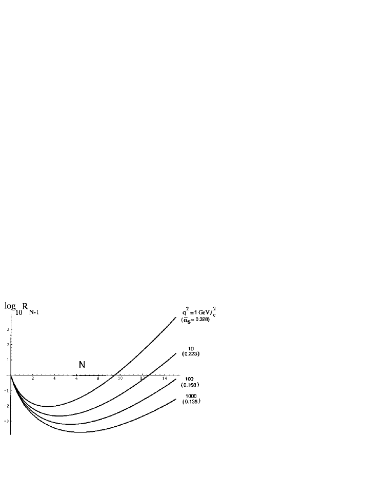
This pattern is shown in Fig. 1 where the error $\bar{R}_{N}$ is plotted versus $N$ for various values of $q^{2}$ with $\Lambda=100$MeV. As can readily be seen from the graph only a very few terms need be retalned in order to get within a few per cent of the correct sum even down to very low values of $q^{2}$. Explicit non-perturbative corrections to the sum arising, for example, from instantons are expected to be of order $e^{-2\pi/\alpha_{s}}$ which is much smaller than even the smallest value of $R_{N}$. This call be put slightly differently by noting that such instanton contributions behave Ilke $(\Lambda^{2}/q^{2})^{-8\pi^{2}b_{1}}$, which remains much smaller than $\bar{R}_{N_{o}}(q^{2})$ down to values of $q^{2}\sim 1$GeV/$c^{2}$. This therefore serves as a possible explanation as to why tree graphs, supplemented by one loop corrections, give such a good description of many processes in QCD even at rather modest energies where $\alpha_{s}$ is relatively large. Both higher order terms and explicit non-perturbative contributions typically contribute less than a per cent; only when one is sensitive to infrared, bound state or threshold problems is it expected that the perturbative description becomes inappropriate.

Finally we should draw attention to the enormous size of the coefficients $r_{N}$ in Table 1; evcntually these lead to contributions that exceed the leading term which, if taken seriously, would invalidate the predictions of asymptotic freedom as is clear from Fig. 1. The technique suggested here says that, in the spirit of asymptotic series, all contributions from diagrams of $O(N_{o})$ and higher should be ignored. It could therefore be argued that, just as in the series (12) where an individual term such as $100!(0.1)^{100}$, for example, should be thought of as irrelevant and meaningless as far as contributing to the ”sum” of the series is concerned, so in (14) 8th order graphs, for example, are likewise meaningless and irrelevant (at least until one gets to sufficiently high energies).

Table 1: The coefficients $r_{N}$ occurring in the expansion of $R$, Eq. (14). The first four are exact while the remaining are estimates from Eq. (15). Also shown are estimates of $R_{N}$, the corresponding deviation from the exact result of the sum of the first $N$ terms of the expansion (calculated using $\alpha_{s}=0.15$). Note that although the $r_{N}$ rapidly diverge, $R_{N}$ goes through a minimum near $N\sim 5$ where the error is only $6.85\times 10^{-4}$.

$N$	$r_{N+1}$	$R_{N}\equiv|r_{N+1}(\alpha_{s}/\pi)^{N+1}|$
$-1$	$1$	$1$
$0$	$1$	$4.77\times 10^{-2}$
$1$	$1.41$	$3.21\times 10^{-3}$
$2$	$12.8$	$1.39\times 10^{-3}$
$3$	$163.4$	$8.49\times 10^{-4}$
$4$	$2.7\times 10^{3}$	$6.71\times 10^{-4}$
$5$	$5.78\times 10^{4}$	$6.85\times 10^{-4}$
$6$	$1.53\times 10^{6}$	$8.63\times 10^{-4}$
$7$	$4.78\times 10^{6}$	$1.29\times 10^{-3}$
$8$	$1.74\times 10^{9}$	$2.25\times 10^{-3}$
$9$	$7.23\times 10^{10}$	$4.45\times 10^{-3}$
$10$	$3.38\times 10^{12}$	$9.93\times 10^{-3}$
$11$	$1.75\times 10^{14}$	$2.45\times 10^{-2}$
$12$	$9.97\times 10^{15}$	$6.68\times 10^{-2}$
$13$	$6.19\times 10^{16}$	$1.98\times 10^{-1}$
$14$	$4.17\times 10^{18}$	$6.38\times 10^{-1}$
$15$	$3.02\times 10^{21}$	$2.2$

REFERENCES AND NOTES

- [1] See, e.g., J. Zinn-Justin, Phys. Rep. 70, 109 (1981) and G. ’t Hooft in Proc. of Orbis Scientiae, Coral Gables, 1977; eds A. Perlmutter and L. F. Scott (Plenum Press, N. Y., 1977), p.699.
- [2] Asymptotic series are discussed in many texts on classical analysis, though typically not in a form that is directly useful for application to quantum field theory. A good standard reference is E. T. Whittaker and G. N. Watson, “A Course in Modern Analysis” (Cambridge University Press, N. Y. 1965).
- [3] G. B. West, Phys. Rev. Letts. 67, 1388 (1991).
- [4] L. N. Lipatov, JETP Lett. 24, 157 (1976).
- [5] When lies along the negative real axis and Im (as for a forward scattering amplitude, for example), a rigorous bound, , can be derived.
- [6] If has a singularity at , then Eq. (10) suggests that there is an explicit non-perturbative contribution to which behaves like . This mimics the situation in QCD where there such explicit contributions () arising from instantons and the like.
- [7] D.T. Barclay and C.J. Maxwell, Phys. Rev. Lett.69, 3417 (1992); L. S. Brown and L. G. Yaffe, Phys. Rev. D4, 398 (1992).