When semantics turns to substance: reformulating QCD analysis of ${\mathbf{F_{2}^{\gamma}(x,Q^{2})}}$

by J. Chรฝla
Institute of Physics, Na Slovance 2, Prague 8, Czech Republic
E-mail
Supported by Grant Agency of ASCR under grant No. A1010602 chyla@fzu.cz
Abstract:

QCD analysis of $F_{2}^{\gamma}(x,Q^{2})$ is revisited. It is emphasized that the presence of the inhomogeneous term in the evolution equations for quark distribution functions of the photon implies important difference in the way factorization mechanism works in photonโ€“hadron and photonโ€“photon collisions as compared to the hadronic ones. Moreover, a careful definitions of the very concepts of the โ€œleading orderโ€ and โ€œnextโ€“toโ€“leading orderโ€ QCD analysis of $F_{2}^{\gamma}$ are needed in order to separate genuine QCD effects from those of pure QED origin. After presenting such definitions, I show that all existing allegedly LO, as well as NLO analyses of $F_{2}^{\gamma}(x,Q^{2})$ are incomplete. The source of this incompleteness of the conventional approach is traced back to the lack of clear identification of QCD effects and to the misinterpretation of the behaviour of $q^{\gamma}(x,M)$ as a function of ฮฑsโ€‹(M)subscript๐›ผ๐‘ ๐‘€\alpha_{s}(M). Complete LO and NLO QCD analyses of $F_{2}^{\gamma}(x,Q^{2})$ are shown to differ substantially from the conventional ones. Whereas complete NLO analysis requires the knowledge of two so far uncalculated quantities, a complete LO one is currently possible, but compared to the conventional formulation requires the inclusion of four known, but in the existing LO analyses unused quantities. The arguments recently advanced in favour of the conventional approach are analyzed and shown to contain a serious flaw. If corrected, they actually lend support to my claim.

QCD, perturbation theory, photon structure
โ€ โ€ preprint: PRA-HEP 99/05

1 Introduction

Observed from a large distance the photon behaves as a neutral structureless object governed by the laws of Quantum Electrodynamics. However, when probed at short distances it exhibits some properties characteristic of hadrons 111For recent theoretical and experimental reviews see [1] and [2, 3], respectively.. This โ€œphoton structureโ€ is quantified, similarly as in the case of hadrons, in terms of parton distribution functions (PDF), satisfying certain evolution equations. Because of the direct coupling of photons to quarkโ€“antiquark pairs these evolution equations are, contrary to the case of hadrons, inhomogeneous. This inhomogeneity has important implications for QCD analysis of $F_{2}^{\gamma}(x,Q^{2})$ and other physical quantities involving photon in the initial state.

In the previous paper [4] these implications led me to the conclusion the all existing NLO QCD analyses of $F_{2}^{\gamma}(x,Q^{2})$ are incomplete. With the exception of the authors of the FKP approach [5] my claim has been either ignored of rejected. The inertia of the โ€œcommon wisdomโ€ is enormous. I have therefore appreciated the recent attempt of A. Vogt [6] to present mathematical arguments in favour of the conventional approach. I analyze them in Section 4 and show that they contain a serious flaw. If corrected, Vogtโ€™s arguments actually lend support to my claim.

In the course of discussions of this and related subjects concerning conventional QCD analysis of photon structure, I have realized that the main source of the confusion surrounding the QCD analysis of $F_{2}^{\gamma}(x,Q^{2})$ was the lack of a clear definition of what โ€œLOโ€ and โ€œNLOโ€ means in the context of photonic interactions. The point is that all existing conventional QCD analyses of $F_{2}^{\gamma}$ mix purely QED effects, which are usually quite dominant, with the genuine QCD ones, which represent mostly small corrections only. I will therefore start by presenting my definition of what โ€œleadingโ€ and โ€œnextโ€“toโ€“leadingโ€ order means for parton distribution functions of the photon and for $F_{2}^{\gamma}(x,Q^{2})$. In the next step I will construct explicit solutions of the inhomogeneous evolution equation including inhomogeneous as well as homogeneous splitting functions up to order ฮฑs2superscriptsubscript๐›ผ๐‘ 2\alpha_{s}^{2}. Straightforward analysis of these solutions shows that my claim in [4] was actually only partially correct: not only the existing supposedly NLO analyses are incomplete, but so are the LO ones! Contrary to the NLO analysis, which is currently impossible to perform because the necessary quantities have not yet been calculated, complete LO QCD analysis of $F_{2}^{\gamma}(x,Q^{2})$ is feasible, but requires the inclusion of several additional Oโ€‹(ฮฑs)๐‘‚subscript๐›ผ๐‘ O(\alpha_{s}) quantities.

The paper is organized as follows. In the next Section basic facts and notation concerning PDF of the photon are recalled, followed in Section 3 by the discussion of the properties of the pointlike part of quark distribution function. Section 4 contains critical analysis of Vogtโ€™s arguments in [6]. In Section 5 the leading and nextโ€“toโ€“leading order QCD analysis of $F_{2}^{\gamma}$ is formulated and the pointlike solutions of the inhomogeneous evolution equation for $q_{\mathrm{NS}}^{\gamma}$ are explicitly written down up to order ฮฑs2superscriptsubscript๐›ผ๐‘ 2\alpha_{s}^{2}. Phenomenological implications of the present analysis for $F_{2}^{\gamma}(x,Q^{2})$ are outlined in Section 6, followed by the summary and conclusions in Section 7. Compared with [4] I have omitted the analysis of the structure of the virtual photon, some of which can be found in [7, 8].

2 Notation and basic facts

In QCD the coupling of quarks and gluons is characterized by the renormalized colour coupling (โ€œcouplantโ€ for short) ฮฑsโ€‹(ฮผ)subscript๐›ผ๐‘ ๐œ‡\alpha_{s}(\mu), depending on the renormalization scale $\mu$ and satisfying the equation

dโ€‹ฮฑsโ€‹(ฮผ)dโ€‹lnโกฮผ2โ‰กฮฒโ€‹(ฮฑsโ€‹(ฮผ))=โˆ’ฮฒ04โ€‹ฯ€โ€‹ฮฑs2โ€‹(ฮผ)โˆ’ฮฒ116โ€‹ฯ€2โ€‹ฮฑs3โ€‹(ฮผ)+โ‹ฏ,dsubscript๐›ผ๐‘ ๐œ‡dsuperscript๐œ‡2๐›ฝsubscript๐›ผ๐‘ ๐œ‡subscript๐›ฝ04๐œ‹superscriptsubscript๐›ผ๐‘ 2๐œ‡subscript๐›ฝ116superscript๐œ‹2superscriptsubscript๐›ผ๐‘ 3๐œ‡โ‹ฏ\frac{{\mathrm{d}}\alpha_{s}(\mu)}{{\mathrm{d}}\ln\mu^{2}}\equiv\beta(\alpha_{s}(\mu))=-\frac{\beta_{0}}{4\pi}\alpha_{s}^{2}(\mu)-\frac{\beta_{1}}{16\pi^{2}}\alpha_{s}^{3}(\mu)+\cdots, (1)

where, in QCD with $n_{f}$ massless quark flavours, the first two coefficients, $\beta_{0}=11-2n_{f}/3$ and $\beta_{1}=102-38n_{f}/3$, are unique, while all the higher order ones are ambiguous. As we shall stay in this paper within the NLO QCD, only the first two, unique, terms in (1) will be taken into account in the following. However, even for a given r.h.s. of (1) its solution ฮฑsโ€‹(ฮผ)subscript๐›ผ๐‘ ๐œ‡\alpha_{s}(\mu) is not a unique function of $\mu$, because there is an infinite number of solutions of (1), differing by the initial condition. This so called renormalization scheme (RS) ambiguity 222In higher orders this ambiguity includes also the arbitrariness of the coefficients $\beta_{i},i\geq 2$. can be parameterized in a number of ways. One of them makes use of the fact that in the process of renormalization another dimensional parameter, denoted usually $\Lambda$, inevitably appears in the theory. This parameter depends on the RS and at the NLO even fully specifies it. For instance, ฮฑsโ€‹(ฮผ)subscript๐›ผ๐‘ ๐œ‡\alpha_{s}(\mu) in the familiar MS and $\overline{\mathrm{MS}}$ RS are two solutions of the same equation (1), associated with different $\Lambda_{\mathrm{RS}}$ 333At the NLO the variation of both the renormalization scale $\mu$ and the renormalization scheme RS$\equiv${$\Lambda_{\mathrm{RS}}$} is redundant. It suffices to fix one of them and vary the other, but I stick to the common practice of considering both of them as free parameters.. In this paper we shall work in the standard $\overline{\mathrm{MS}}$ RS of the couplant.

โ€œDressedโ€ PDF 444In the following the adjective โ€œdressedโ€ as well as the superscript โ€œฮณ๐›พ\gammaโ€ will be dropped. result from the resummation of multiple parton collinear emission off the corresponding โ€œbareโ€ parton distributions. As a result of this resummation PDF acquire dependence on the factorization scale $M$. This scale defines the upper limit on some measure $t$ of the offโ€“shellness of partons included in the definition of $D(x,M)$

$$D_{i}(x,M)\equiv\int_{t_{\mathrm{min}}}^{M^{2}}{\mathrm{d}}td_{i}(x,t),~{}~{}~{}~{}~{}~{}i=q,\overline{q},G,$$ (2)

where the unintegrated PDF $d_{i}(x,t)$ describe distribution functions of partons with the momentum fraction $x$ and fixed offโ€“shellness $t$. Parton virtuality $\tau\equiv\mid p^{2}-m^{2}\mid$ or transverse mass $m_{T}^{2}\equiv p_{T}^{2}+m^{2}$, are two standard choices of such a measure. Because at small $t$, $d_{i}(x,t)={\cal O}(1/t^{k}),k=1,2$, the dominant part of the integral (2) comes from the region of small offโ€“shellness $t$. Varying the upper bound $M^{2}$ in (2) has therefore only a small effect on the integral (2), leading to weak (at most logarithmic) scaling violations. Factorization scale dependence of PDF of the photon 555If not stated otherwise all distribution functions in the following concern the photon. is determined by the system of coupled inhomogeneous evolution equations

$\displaystyle\frac{{\mathrm{d}}\Sigma(x,M)}{{\mathrm{d}}\ln M^{2}}$ $\displaystyle=$ $\displaystyle\delta_{\Sigma}k_{q}+P_{qq}\otimes\Sigma+P_{qG}\otimes G,$ (3)
$\displaystyle\frac{{\mathrm{d}}G(x,M)}{{\mathrm{d}}\ln M^{2}}$ $\displaystyle=$ $\displaystyle k_{G}+P_{Gq}\otimes\Sigma+P_{GG}\otimes G,$ (4)
$\displaystyle\frac{{\mathrm{d}}q_{\mathrm{NS}}(x,M)}{{\mathrm{d}}\ln M^{2}}$ $\displaystyle=$ $\displaystyle\delta_{\mathrm{NS}}k_{q}+P_{\mathrm{NS}}\otimes q_{\mathrm{NS}},$ (5)

where 666For nonsinglet quark distribution function $q_{\mathrm{NS}}$ another definition is used in the literature [9]. The definition adopted here corresponds to that used in [10].

$\displaystyle\Sigma(x,M)$ $\displaystyle\equiv$ $\displaystyle\sum_{i=1}^{n_{f}}q_{i}^{+}(x,M)\equiv\sum_{i=1}^{n_{f}}\left[q_{i}(x,M)+\overline{q}_{i}(x,M)\right],$ (6)
$\displaystyle q_{\mathrm{NS}}(x,M)$ $\displaystyle\equiv$ $\displaystyle\sum_{i=1}^{n_{f}}\left(e_{i}^{2}-\langle e^{2}\rangle\right)\left(q_{i}(x,M)+\overline{q}_{i}(x,M)\right),$ (7)
$$\delta_{\mathrm{NS}}=6n_{f}\left(\langle e^{4}\rangle-\langle e^{2}\rangle^{2}\right),~{}~{}~{}\delta_{\Sigma}=6n_{f}\langle e^{2}\rangle.$$ (8)

To order $\alpha$ the splitting functions $P_{ij}$ and $k_{i}$ are given as power expansions in ฮฑsโ€‹(M)subscript๐›ผ๐‘ ๐‘€\alpha_{s}(M):

$\displaystyle k_{q}(x,M)$ $\displaystyle=$ ฮฑ2โ€‹ฯ€โ€‹[kq(0)โ€‹(x)+ฮฑsโ€‹(M)2โ€‹ฯ€โ€‹kq(1)โ€‹(x)+(ฮฑsโ€‹(M)2โ€‹ฯ€)2โ€‹kq(2)โ€‹(x)+โ‹ฏ],๐›ผ2๐œ‹delimited-[]subscriptsuperscript๐‘˜0๐‘ž๐‘ฅsubscript๐›ผ๐‘ ๐‘€2๐œ‹superscriptsubscript๐‘˜๐‘ž1๐‘ฅsuperscriptsubscript๐›ผ๐‘ ๐‘€2๐œ‹2subscriptsuperscript๐‘˜2๐‘ž๐‘ฅโ‹ฏ\displaystyle\frac{\alpha}{2\pi}\left[k^{(0)}_{q}(x)+\frac{\alpha_{s}(M)}{2\pi}k_{q}^{(1)}(x)+\left(\frac{\alpha_{s}(M)}{2\pi}\right)^{2}k^{(2)}_{q}(x)+\cdots\right], (9)
$\displaystyle k_{G}(x,M)$ $\displaystyle=$ ฮฑ2โ€‹ฯ€โ€‹[ฮฑsโ€‹(M)2โ€‹ฯ€โ€‹kG(1)โ€‹(x)+(ฮฑsโ€‹(M)2โ€‹ฯ€)2โ€‹kG(2)โ€‹(x)+โ‹ฏ],๐›ผ2๐œ‹delimited-[]subscript๐›ผ๐‘ ๐‘€2๐œ‹superscriptsubscript๐‘˜๐บ1๐‘ฅsuperscriptsubscript๐›ผ๐‘ ๐‘€2๐œ‹2subscriptsuperscript๐‘˜2๐บ๐‘ฅโ‹ฏ\displaystyle\frac{\alpha}{2\pi}\left[~{}~{}~{}~{}~{}~{}~{}~{}~{}~{}~{}~{}\frac{\alpha_{s}(M)}{2\pi}k_{G}^{(1)}(x)+\left(\frac{\alpha_{s}(M)}{2\pi}\right)^{2}k^{(2)}_{G}(x)+\cdots\;\right], (10)
$\displaystyle P_{ij}(x,M)$ $\displaystyle=$ ฮฑsโ€‹(M)2โ€‹ฯ€โ€‹Piโ€‹j(0)โ€‹(x)+(ฮฑsโ€‹(M)2โ€‹ฯ€)2โ€‹Piโ€‹j(1)โ€‹(x)+โ‹ฏ,subscript๐›ผ๐‘ ๐‘€2๐œ‹subscriptsuperscript๐‘ƒ0๐‘–๐‘—๐‘ฅsuperscriptsubscript๐›ผ๐‘ ๐‘€2๐œ‹2superscriptsubscript๐‘ƒ๐‘–๐‘—1๐‘ฅโ‹ฏ\displaystyle~{}~{}~{}~{}~{}~{}~{}~{}~{}~{}~{}~{}~{}~{}~{}~{}~{}~{}\frac{\alpha_{s}(M)}{2\pi}P^{(0)}_{ij}(x)+\left(\frac{\alpha_{s}(M)}{2\pi}\right)^{2}P_{ij}^{(1)}(x)+\cdots, (11)

where the leading order splitting functions $k_{q}^{(0)}(x)=(x^{2}+(1-x)^{2})$ and $P^{(0)}_{ij}(x)$ are unique, while all higher order ones $k^{(j)}_{q},k^{(j)}_{G},P^{(j)}_{kl},j\geq 1$ depend on the choice of the factorization scheme (FS). The equations (3-5) can be recast into evolution equations for $q_{i}(x,M),\overline{q}_{i}(x,M)$ and $G(x,M)$ with inhomegenous splitting functions $k_{q_{i}}^{(0)}=3e_{i}^{2}k_{q}^{(0)}$. The photon structure function $F_{2}^{\gamma}(x,Q^{2})$, measured in deep inelastic scattering of electrons on photons is given as

$\displaystyle\frac{1}{x}F_{2}^{\gamma}(x,Q^{2})$ $\displaystyle=$ $\displaystyle q_{\mathrm{NS}}(M)\otimes C_{q}(Q/M)+\frac{\alpha}{2\pi}\delta_{\mathrm{NS}}C_{\gamma}+$ (13)
โŸจe2โŸฉโ€‹ฮฃโ€‹(M)โŠ—Cqโ€‹(Q/M)+ฮฑ2โ€‹ฯ€โ€‹โŸจe2โŸฉโ€‹ฮดฮฃโ€‹Cฮณ+โŸจe2โŸฉโ€‹ฮฑs2โ€‹ฯ€โ€‹Gโ€‹(M)โŠ—CGโ€‹(Q/M)tensor-productdelimited-โŸจโŸฉsuperscript๐‘’2ฮฃ๐‘€subscript๐ถ๐‘ž๐‘„๐‘€๐›ผ2๐œ‹delimited-โŸจโŸฉsuperscript๐‘’2subscript๐›ฟฮฃsubscript๐ถ๐›พtensor-productdelimited-โŸจโŸฉsuperscript๐‘’2subscript๐›ผ๐‘ 2๐œ‹๐บ๐‘€subscript๐ถ๐บ๐‘„๐‘€\displaystyle\langle e^{2}\rangle\Sigma(M)\otimes C_{q}(Q/M)+\frac{\alpha}{2\pi}\langle e^{2}\rangle\delta_{\Sigma}C_{\gamma}+\langle e^{2}\rangle\frac{\alpha_{s}}{2\pi}G(M)\otimes C_{G}(Q/M)

of photonic PDF and coefficient functions $C_{q}(x),C_{G}(x),C_{\gamma}(x)$ admitting perturbative expansions

$\displaystyle C_{q}(x,Q/M)$ $\displaystyle=$ ฮดโ€‹(1โˆ’x)+ฮฑsโ€‹(ฮผ)2โ€‹ฯ€โ€‹Cq(1)โ€‹(x,Q/M)+โ‹ฏ,๐›ฟ1๐‘ฅsubscript๐›ผ๐‘ ๐œ‡2๐œ‹subscriptsuperscript๐ถ1๐‘ž๐‘ฅ๐‘„๐‘€โ‹ฏ\displaystyle\delta(1-x)~{}~{}~{}~{}+~{}~{}~{}\frac{\alpha_{s}(\mu)}{2\pi}C^{(1)}_{q}(x,Q/M)+\cdots, (14)
$\displaystyle C_{G}(x,Q/M)$ $\displaystyle=$ ฮฑsโ€‹(ฮผ)2โ€‹ฯ€โ€‹CG(1)โ€‹(x,Q/M)+โ‹ฏ,subscript๐›ผ๐‘ ๐œ‡2๐œ‹subscriptsuperscript๐ถ1๐บ๐‘ฅ๐‘„๐‘€โ‹ฏ\displaystyle~{}~{}~{}~{}~{}~{}~{}~{}~{}~{}~{}~{}~{}~{}~{}~{}~{}~{}~{}~{}~{}\frac{\alpha_{s}(\mu)}{2\pi}C^{(1)}_{G}(x,Q/M)+\cdots, (15)
$\displaystyle C_{\gamma}(x,Q/M)$ $\displaystyle=$ Cฮณ(0)โ€‹(x,Q/M)+ฮฑsโ€‹(ฮผ)2โ€‹ฯ€โ€‹Cฮณ(1)โ€‹(x,Q/M)+โ‹ฏ,superscriptsubscript๐ถ๐›พ0๐‘ฅ๐‘„๐‘€subscript๐›ผ๐‘ ๐œ‡2๐œ‹superscriptsubscript๐ถ๐›พ1๐‘ฅ๐‘„๐‘€โ‹ฏ\displaystyle C_{\gamma}^{(0)}(x,Q/M)+\frac{\alpha_{s}(\mu)}{2\pi}C_{\gamma}^{(1)}(x,Q/M)+\cdots, (16)

where the standard formula for $C_{\gamma}^{(0)}$ reads 777Alternatives to this expression for $Q^{2}=M^{2}$ are discussed in Subsection 6.6.

$$C_{\gamma}^{(0)}(x,Q/M)=\left(x^{2}+(1-x)^{2}\right)\left[\ln\frac{M^{2}}{Q^{2}}+\ln\frac{1-x}{x}\right]+8x(1-x)-1.$$ (17)

The renormalization scale $\mu$, used as argument of ฮฑsโ€‹(ฮผ)subscript๐›ผ๐‘ ๐œ‡\alpha_{s}(\mu) in (14-16) is in principle independent of the factorization scale $M$. Note that despite the presence of $\mu$ as argument of ฮฑsโ€‹(ฮผ)subscript๐›ผ๐‘ ๐œ‡\alpha_{s}(\mu) in (14โ€“16), the coefficient functions $C_{q},C_{G}$ and $C_{\gamma}$ are actually independent of $\mu$ because the $\mu$โ€“dependence of the expansion parameter ฮฑsโ€‹(ฮผ)subscript๐›ผ๐‘ ๐œ‡\alpha_{s}(\mu) is cancelled by explicit dependence of $C^{(i)}_{q},C^{(i)}_{G},C^{(i)}_{\gamma},i\geq 2$ on $\mu$ [11]. On the other hand, PDF and the coefficient functions $C_{q},C_{G}$ and $C_{\gamma}$ do depend on both the factorization scale $M$ and factorization scheme, but in such a correlated manner that physical quantities, like $F_{2}^{\gamma}$, are independent of both $M$ and the FS, provided expansions (9โ€“11) and (14โ€“16) are taken to all orders in ฮฑsโ€‹(M)subscript๐›ผ๐‘ ๐‘€\alpha_{s}(M) and ฮฑsโ€‹(ฮผ)subscript๐›ผ๐‘ ๐œ‡\alpha_{s}(\mu). In practical calculations based on truncated forms of (9โ€“11) and (14โ€“16) this invariance is, however, lost and the choice of both $M$ and FS makes numerical difference even for physical quantities. The expressions for $C_{q}^{(1)},C^{(1)}_{G}$ given in [12] are usually claimed to correspond to โ€œMSยฏยฏMS\overline{\mathrm{MS}} factorization schemeโ€. As argued in [13], this denomination is, however, incomplete. The adjective โ€œMSยฏยฏMS\overline{\mathrm{MS}}โ€ concerns exclusively the choice of the RS of the couplant ฮฑssubscript๐›ผ๐‘ \alpha_{s} and has nothing to do with the choice of the splitting functions $P^{(1)}_{ij}$. The choices of the renormalization scheme of the couplant ฮฑssubscript๐›ผ๐‘ \alpha_{s} and of the factorization scheme of PDF are two completely independent decisions, concerning two different and in general unrelated redefinition procedures. Both are necessary in order to specify uniquely the results of fixed order perturbative calculations, but we may combine any choice of the RS of the couplant with any choice of the FS of PDF. The coefficient functions $C_{q},C_{G},C_{\gamma}$ depend on both of them, whereas the splitting functions depend only on the latter. The results given in [12] correspond to $\overline{\mathrm{MS}}$ RS of the couplant but to the โ€œminimal subtractionโ€ FS of PDF 888See Section 2.6 of [14], in particular eq. (2.31), for discussion of this point.. It is therefore more appropriate to call this full specification of the renormalization and factorization schemes as โ€œMSยฏ+MSยฏMSMS\overline{\mathrm{MS}}+{\mathrm{MS}} schemeโ€. Although the phenomenological relevance of treating $\mu$ and $M$ as independent parameters has been demonstrated [15], I shall follow the usual practice and set $\mu=M$.

3 Pointlike solutions and their properties

The general solution of the evolution equations (3-5) can be written as the sum of a particular solution of the full inhomogeneous equation and the general solution of the corresponding homogeneous one, called hadronic 999Sometimes also called โ€œVDM partโ€ because it is usually modelled by PDF of vector mesons. part. A subset of the solutions of full evolution equations resulting from the resummation of series of diagrams like those in Fig. (1), which start with the pointlike purely QED vertex $\gamma\rightarrow q\overline{q}$, are called pointlike (PL) solutions. In writing down the expression for the resummation of diagrams in Fig. 1 there is a freedom in specifying some sort of boundary condition. It is common to work within a subset of pointlike solutions specified by the value of the scale $M_{0}$ at which they vanish. In general, we can thus write ($D=q,\overline{q},G$)

$$D(x,M^{2})=D^{\mathrm{PL}}(x,M^{2})+D^{\mathrm{HAD}}(x,M^{2}).$$ (18)

Due to the fact that there is an infinite number of pointlike solutions $q^{\mathrm{PL}}(x,M^{2})$, the separation of quark and gluon distribution functions into their pointlike and hadronic parts is, however, ambiguous and therefore these concepts have separately no physical meaning. In [7] we discussed numerical aspects of this ambiguity for the Schulerโ€“Sjรถstrand sets of parameterizations [16].

Refer to caption
Figure 1: Diagrams defining the pointlike parts of NS quark distribution function in LL approximation. The resummation involves integration over parton virtualities $M_{0}^{2}\leq\tau\leq M^{2}$..

To see the most important feature of the pointlike part of quark distribution functions that will be crucial for the following analysis, let us consider in detail the case of nonsinglet quark distribution function $q_{\mathrm{NS}}(x,M)$, which is explicitly defined via the series

qNSPLโ€‹(x,M0,M)โ‰กฮฑ2โ€‹ฯ€โ€‹kNS(0)โ€‹(x)โ€‹โˆซM02M2dโ€‹ฯ„ฯ„+โˆซx1dโ€‹yyโ€‹Pqโ€‹q(0)โ€‹(xy)โ€‹โˆซM02M2dโ€‹ฯ„1ฯ„1โ€‹ฮฑsโ€‹(ฯ„1)2โ€‹ฯ€โ€‹ฮฑ2โ€‹ฯ€โ€‹kNS(0)โ€‹(y)โ€‹โˆซM02ฯ„1dโ€‹ฯ„2ฯ„2+subscriptsuperscript๐‘žPLNS๐‘ฅsubscript๐‘€0๐‘€๐›ผ2๐œ‹superscriptsubscript๐‘˜NS0๐‘ฅsubscriptsuperscriptsuperscript๐‘€2superscriptsubscript๐‘€02d๐œ๐œlimit-fromsubscriptsuperscript1๐‘ฅd๐‘ฆ๐‘ฆsubscriptsuperscript๐‘ƒ0๐‘ž๐‘ž๐‘ฅ๐‘ฆsubscriptsuperscriptsuperscript๐‘€2superscriptsubscript๐‘€02dsubscript๐œ1subscript๐œ1subscript๐›ผ๐‘ subscript๐œ12๐œ‹๐›ผ2๐œ‹superscriptsubscript๐‘˜NS0๐‘ฆsubscriptsuperscriptsubscript๐œ1superscriptsubscript๐‘€02dsubscript๐œ2subscript๐œ2q^{\mathrm{PL}}_{\mathrm{NS}}(x,M_{0},M)\equiv\frac{\alpha}{2\pi}k_{\mathrm{NS}}^{(0)}(x)\int^{M^{2}}_{M_{0}^{2}}\frac{{\mathrm{d}}\tau}{\tau}+\int^{1}_{x}\frac{{\mathrm{d}}y}{y}P^{(0)}_{qq}\left(\frac{x}{y}\right)\int^{M^{2}}_{M_{0}^{2}}\frac{{\mathrm{d}}\tau_{1}}{\tau_{1}}\frac{\alpha_{s}(\tau_{1})}{2\pi}\frac{\alpha}{2\pi}k_{\mathrm{NS}}^{(0)}(y)\int^{\tau_{1}}_{M_{0}^{2}}\frac{{\mathrm{d}}\tau_{2}}{\tau_{2}}+
โˆซx1dโ€‹yyโ€‹Pqโ€‹q(0)โ€‹(xy)โ€‹โˆซy1dโ€‹wwโ€‹Pqโ€‹q(0)โ€‹(yw)โ€‹โˆซM02M2dโ€‹ฯ„1ฯ„1โ€‹ฮฑsโ€‹(ฯ„1)2โ€‹ฯ€โ€‹โˆซM02ฯ„1dโ€‹ฯ„2ฯ„2โ€‹ฮฑsโ€‹(ฯ„2)2โ€‹ฯ€โ€‹ฮฑ2โ€‹ฯ€โ€‹kNS(0)โ€‹(w)โ€‹โˆซM02ฯ„2dโ€‹ฯ„3ฯ„3+โ‹ฏ,subscriptsuperscript1๐‘ฅd๐‘ฆ๐‘ฆsubscriptsuperscript๐‘ƒ0๐‘ž๐‘ž๐‘ฅ๐‘ฆsubscriptsuperscript1๐‘ฆd๐‘ค๐‘คsubscriptsuperscript๐‘ƒ0๐‘ž๐‘ž๐‘ฆ๐‘คsubscriptsuperscriptsuperscript๐‘€2superscriptsubscript๐‘€02dsubscript๐œ1subscript๐œ1subscript๐›ผ๐‘ subscript๐œ12๐œ‹subscriptsuperscriptsubscript๐œ1superscriptsubscript๐‘€02dsubscript๐œ2subscript๐œ2subscript๐›ผ๐‘ subscript๐œ22๐œ‹๐›ผ2๐œ‹superscriptsubscript๐‘˜NS0๐‘คsubscriptsuperscriptsubscript๐œ2superscriptsubscript๐‘€02dsubscript๐œ3subscript๐œ3โ‹ฏ\int^{1}_{x}\frac{{\mathrm{d}}y}{y}P^{(0)}_{qq}\left(\frac{x}{y}\right)\int^{1}_{y}\frac{{\mathrm{d}}w}{w}P^{(0)}_{qq}\left(\frac{y}{w}\right)\int^{M^{2}}_{M_{0}^{2}}\frac{{\mathrm{d}}\tau_{1}}{\tau_{1}}\frac{\alpha_{s}(\tau_{1})}{2\pi}\int^{\tau_{1}}_{M_{0}^{2}}\frac{{\mathrm{d}}\tau_{2}}{\tau_{2}}\frac{\alpha_{s}(\tau_{2})}{2\pi}\frac{\alpha}{2\pi}k_{\mathrm{NS}}^{(0)}(w)\int^{\tau_{2}}_{M_{0}^{2}}\frac{{\mathrm{d}}\tau_{3}}{\tau_{3}}+\cdots, (19)

where $k_{\mathrm{NS}}^{(0)}(x)=\delta_{\mathrm{NS}}k^{(0)}_{q}(x)$. In terms of moments defined as

$$f(n)\equiv\int_{0}^{1}x^{n}f(x)\mathrm{d}x$$ (20)

this series can be resummed in a closed form

qNSPLโ€‹(n,M0,M)=4โ€‹ฯ€ฮฑsโ€‹(M)โ€‹[1โˆ’(ฮฑsโ€‹(M)ฮฑsโ€‹(M0))1โˆ’2โ€‹Pqโ€‹q(0)โ€‹(n)/ฮฒ0]โ€‹aNSโ€‹(n),superscriptsubscript๐‘žNSPL๐‘›subscript๐‘€0๐‘€4๐œ‹subscript๐›ผ๐‘ ๐‘€delimited-[]1superscriptsubscript๐›ผ๐‘ ๐‘€subscript๐›ผ๐‘ subscript๐‘€012subscriptsuperscript๐‘ƒ0๐‘ž๐‘ž๐‘›subscript๐›ฝ0subscript๐‘ŽNS๐‘›q_{\mathrm{NS}}^{\mathrm{PL}}(n,M_{0},M)=\frac{4\pi}{\alpha_{s}(M)}\left[1-\left(\frac{\alpha_{s}(M)}{\alpha_{s}(M_{0})}\right)^{1-2P^{(0)}_{qq}(n)/\beta_{0}}\right]a_{\mathrm{NS}}(n), (21)

where

$$a_{\mathrm{NS}}(n)\equiv\frac{\alpha}{2\pi\beta_{0}}\frac{k_{\mathrm{NS}}^{(0)}(n)}{1-2P^{(0)}_{qq}(n)/\beta_{0}}.$$ (22)
Refer to caption
Figure 2: Comparison, left in the nonsinglet and right in the singlet channels, of the functions $xk_{i}(x)=x\delta_{i}k_{q}^{(0)},i=\mathrm{NS},\Sigma$ with the functions $xa(x)$ corresponding to asymptotic pointlike solutions (23) and its analogue in the singlet channel.

It is straightforward to show that (19) or, equivalently, (21), satisfy the evolution equation (5) with the splitting functions $k_{q}$ and $P_{ij}$ including the first terms $k_{q}^{(0)}$ and $P_{qq}^{(0)}$ only.

Transforming (22) to the $x$โ€“space by means of inverse Mellin transformation we get $a_{\mathrm{NS}}(x)$ shown in Fig. 2. The resummation softens the $x-$dependence of $a_{\mathrm{NS}}(x)$ with respect to the first term in (19), proportional to $k_{\mathrm{NS}}(x)$, but does not change the logarithmic dependence of $q_{\mathrm{NS}}$ on $M$. In the nonsinglet channel the effects of gluon radiation on $q_{\mathrm{NS}}^{\mathrm{PL}}$ are significant for $x>0.6$ but small elsewhere, whereas in the singlet channel such effects are marked also for $x<0.5$, where they lead to a steep rise of $xq_{\mathrm{NS}}^{\mathrm{PL}}$ at very small $x$. As emphasized long time ago by authors of [5] the logarithmic dependence of $q_{\mathrm{NS}}^{\mathrm{PL}}$ on $\ln M$ has nothing to do with QCD and results exclusively from integration over the transverse momenta (virtualities) of quarks coming from the basic QED $\gamma\rightarrow q\overline{q}$ splitting. For $M/M_{0}\rightarrow\infty$ the second term in brackets of (21) vanishes and therefore all pointlike solutions share the same large $M$ behaviour

qNSPLโ€‹(x,M0,M)โ†’4โ€‹ฯ€ฮฑsโ€‹(M)โ€‹aNSโ€‹(x)โ‰กqNSAPโ€‹(x,M)โˆlnโกM2ฮ›2,โ†’subscriptsuperscript๐‘žPLNS๐‘ฅsubscript๐‘€0๐‘€4๐œ‹subscript๐›ผ๐‘ ๐‘€subscript๐‘ŽNS๐‘ฅsubscriptsuperscript๐‘žAPNS๐‘ฅ๐‘€proportional-tosuperscript๐‘€2superscriptฮ›2q^{\mathrm{PL}}_{\mathrm{NS}}(x,M_{0},M)\rightarrow\frac{4\pi}{\alpha_{s}(M)}a_{\mathrm{NS}}(x)\equiv q^{\mathrm{AP}}_{\mathrm{NS}}(x,M)\propto\ln\frac{M^{2}}{\Lambda^{2}}, (23)

defining the so called asymptotic pointlike solution $q^{\mathrm{AP}}_{\mathrm{NS}}(x,M)$ [17, 18]. Note that (23) can be interpreted as a special case of the general pointlike solution (21) in which the lower integration limit $M_{0}$ in (19) is set equal to $\Lambda$, i.e. $M_{0}=\Lambda$! The fact that for the asymptotic pointlike solution (23) ฮฑsโ€‹(M)subscript๐›ผ๐‘ ๐‘€\alpha_{s}(M) appears in the denominator of (23) has been the source of misleading claims (see, for instance, [1]) that qโ€‹(x,M)=๐’ชโ€‹(1/ฮฑs)๐‘ž๐‘ฅ๐‘€๐’ช1subscript๐›ผ๐‘ q(x,M)={\cal O}(1/\alpha_{s}). This claim is wrong for a number of reasons. First, it is manifestly invalid for the widely used Schulerโ€“Sjรถstrand SaS1 and SaS2 sets, which take $M_{0}=0.6$ GeV and $M_{0}=2$ GeV. It is obvious [19] that provided $M_{0}$ is kept fixed when ฮฑsโ†’0โ†’subscript๐›ผ๐‘ 0\alpha_{s}\rightarrow 0 the sum (19) approaches its first term, i.e.

$$q^{\mathrm{PL}}_{\mathrm{NS}}(x,M,M_{0})\rightarrow\frac{\alpha}{2\pi}k_{\mathrm{NS}}^{(0)}(x)\ln\frac{M^{2}}{M_{0}^{2}},$$ (24)

corresponding to purely QED splitting $\gamma\rightarrow q\overline{q}$. However, the claim that qโˆ1/ฮฑsproportional-to๐‘ž1subscript๐›ผ๐‘ q\propto 1/\alpha_{s} is misleading even for the asymptotic pointlike solution (23). The fact that it diverges when $\Lambda\rightarrow 0$ is a direct consequence of the fact that for this (and only this) pointlike solution the decrease of the coupling ฮฑsโ€‹(M/ฮ›)subscript๐›ผ๐‘ ๐‘€ฮ›\alpha_{s}(M/\Lambda) as $\Lambda\rightarrow 0$ is compensated by the simultaneous extension of the integration region as $M_{0}=\Lambda\rightarrow 0$! If, however, QCD is switched off by sending $\Lambda\rightarrow 0$ without simultaneously extending the integration region, i.e. for fixed $M_{0}$, there is no trace of QCD left and we get back the simple QED formula (24). This suggests to identify QCD contribution to NS quark distribution function with the difference

$$q^{\mathrm{QCD}}_{\mathrm{NS}}(x,M)\equiv q_{\mathrm{NS}}^{\mathrm{PL}}(x,M_{0},M)-\frac{\alpha}{2\pi}k_{\mathrm{NS}}^{(0)}(x)\ln\frac{M^{2}}{M_{0}^{2}}.$$ (25)

Expanding (21) in powers of ฮฑsโ€‹(M)subscript๐›ผ๐‘ ๐‘€\alpha_{s}(M), keeping $M_{0}$ and $M$ fixed we find

qNSQCDโ€‹(n,M)=ฮฑ2โ€‹ฯ€โ€‹ฮฑs2โ€‹ฯ€โ€‹kq(0)โ€‹(n)โ€‹Pqโ€‹q(0)โ€‹(n)2โ€‹ln2โกM2M02+Oโ€‹(ฮฑs2),subscriptsuperscript๐‘žQCDNS๐‘›๐‘€๐›ผ2๐œ‹subscript๐›ผ๐‘ 2๐œ‹superscriptsubscript๐‘˜๐‘ž0๐‘›superscriptsubscript๐‘ƒ๐‘ž๐‘ž0๐‘›2superscript2superscript๐‘€2superscriptsubscript๐‘€02๐‘‚superscriptsubscript๐›ผ๐‘ 2q^{\mathrm{QCD}}_{\mathrm{NS}}(n,M)=\frac{\alpha}{2\pi}\frac{\alpha_{s}}{2\pi}\frac{k_{q}^{(0)}(n)P_{qq}^{(0)}(n)}{2}\ln^{2}\frac{M^{2}}{M_{0}^{2}}+O(\alpha_{s}^{2}), (26)

as expected from the explicit expression for the second term on the r.h.s. of (19). Note that the leading term in (26) is proportional to the second power of $L_{M}\equiv\ln(M^{2}/M_{0}^{2})$. In subsection 5.2.2 I will argue that in a complete LO QCD analysis $q_{\mathrm{NS}}$ contains another term that behaves as ฮฑsโ€‹LMsubscript๐›ผ๐‘ subscript๐ฟ๐‘€\alpha_{s}L_{M}.

In summary, $q^{\mathrm{PL}}_{\mathrm{NS}}(x,M)$ can be written a sum of two terms: purely QED contribution, proportional to $\alpha$, and the term describing genuine QCD effects, proportional to ฮฑโ€‹ฮฑs๐›ผsubscript๐›ผ๐‘ \alpha\alpha_{s} and thus vanishing when QCD is switched off. One can use the usual claim that qโˆฮฑ/ฮฑsproportional-to๐‘ž๐›ผsubscript๐›ผ๐‘ q\propto\alpha/\alpha_{s} merely as a shorthand for the specification of large $M$ behaviour of (19), as expressed in (23). In fact, this is in fact what one finds in the original papers [17, 18]101010See, for instance, eq. (3.20) of [18]. which do not contain any explicit claim that qโ€‹(x,M)=๐’ชโ€‹(1/ฮฑs)๐‘ž๐‘ฅ๐‘€๐’ช1subscript๐›ผ๐‘ q(x,M)={\cal O}(1/\alpha_{s}).

4 What is proving Vogtโ€™s proof?

Before presenting my reformulation of the LO and NLO QCD analysis of $F_{2}^{\gamma}$, let me go through Vogtโ€™s arguments 111111Note that due to slightly different notation my $C_{\gamma}^{(0)}$ plays the role of $C_{\gamma}^{(1)}$ in [6]. that purport to prove that qโ€‹(M)โˆฮฑ/ฮฑsproportional-to๐‘ž๐‘€๐›ผsubscript๐›ผ๐‘ q(M)\propto\alpha/\alpha_{s}. For the purpose of the discussion in this Section I will adopt Vogtโ€™s simplified notation, in which asโ‰กฮฑs/4โ€‹ฯ€subscript๐‘Ž๐‘ subscript๐›ผ๐‘ 4๐œ‹a_{s}\equiv\alpha_{s}/4\pi, $F^{\gamma}\equiv F_{2,{\mathrm{NS}}}^{\gamma}/\alpha$, $q^{\gamma}\equiv q_{\mathrm{NS}}^{\gamma}$ and ${\mathrm{d}}F^{\gamma}/{\mathrm{d}}\ln Q^{2}=\dot{F}^{\gamma}$, all obvious indices as well as overall charge factors are suppressed and products of $x$โ€“dependent quantities are understood as convolutions in $x$ space or simple products in momentum space. We have

$\displaystyle F^{\gamma}$ $\displaystyle=$ $\displaystyle C_{q}q^{\gamma}+C_{\gamma}$ (27)
$\displaystyle\dot{q}^{\gamma}$ $\displaystyle=$ $\displaystyle k+Pq^{\gamma}$ (28)
$\displaystyle\dot{F}^{\gamma}$ $\displaystyle=$ $\displaystyle\dot{C}_{q}q^{\gamma}+C_{q}\dot{q}^{\gamma}+\dot{C}_{\gamma}$ (29)

The r.h.s. of (29) can be rewritten as [6]

$$\dot{F}^{\gamma}=\left(-\dot{C}_{q}C_{q}^{-1}C_{\gamma}+C_{q}k-PC_{\gamma}+\dot{C}_{\gamma}\right)+\left(\dot{C}_{q}C_{q}^{-1}+P\right)F^{\gamma},$$ (30)

where expressions in the brackets are factorization scheme invariants. Inserting into (30) perturbation expansions of $C_{q},C_{\gamma}$, their derivatives and the splitting functions $k,~{}P$ we get 121212 Note that eq. (14) of [6] contains two misprints in the bracket standing by as2superscriptsubscript๐‘Ž๐‘ 2a_{s}^{2}: the last term comes with the wrong sign and the preceding one should correctly read $-\beta_{0}C_{\gamma}^{(2)}$ (my $C_{\gamma}^{(1)}$ and $C_{\gamma}^{(0)}$ correspond to $C_{\gamma}^{(2)}$ and $C_{\gamma}^{(1)}$ in Vogtโ€™s notation).

Fห™ฮณ=(as)0โ€‹k(0)superscriptห™๐น๐›พsuperscriptsubscript๐‘Ž๐‘ 0superscript๐‘˜0\displaystyle\dot{F}^{\gamma}=~{}~{}(a_{s})^{0}k^{(0)}
+(as)1โ€‹[k(1)+Cq(1)โ€‹k(0)โˆ’P(0)โ€‹Cฮณ(0)]superscriptsubscript๐‘Ž๐‘ 1delimited-[]superscript๐‘˜1superscriptsubscript๐ถ๐‘ž1superscript๐‘˜0superscript๐‘ƒ0superscriptsubscript๐ถ๐›พ0\displaystyle+(a_{s})^{1}\left[k^{(1)}+C_{q}^{(1)}k^{(0)}-P^{(0)}C_{\gamma}^{(0)}\right]
+(as)2โ€‹[k(2)+Cq(1)โ€‹k(1)+Cq(2)โ€‹k(0)โˆ’P(0)โ€‹Cฮณ(1)โˆ’P(1)โ€‹Cฮณ(0)โˆ’ฮฒ0โ€‹Cฮณ(1)+ฮฒ0โ€‹Cq(1)โ€‹Cฮณ(0)]superscriptsubscript๐‘Ž๐‘ 2delimited-[]superscript๐‘˜2superscriptsubscript๐ถ๐‘ž1superscript๐‘˜1superscriptsubscript๐ถ๐‘ž2superscript๐‘˜0superscript๐‘ƒ0superscriptsubscript๐ถ๐›พ1superscript๐‘ƒ1superscriptsubscript๐ถ๐›พ0subscript๐›ฝ0superscriptsubscript๐ถ๐›พ1subscript๐›ฝ0subscriptsuperscript๐ถ1๐‘žsubscriptsuperscript๐ถ0๐›พ\displaystyle+(a_{s})^{2}\left[k^{(2)}+C_{q}^{(1)}k^{(1)}+C_{q}^{(2)}k^{(0)}-P^{(0)}C_{\gamma}^{(1)}-P^{(1)}C_{\gamma}^{(0)}-\beta_{0}C_{\gamma}^{(1)}+\beta_{0}C^{(1)}_{q}C^{(0)}_{\gamma}\right]
+Fฮณโ€‹[asโ€‹P(0)+โ‹ฏ].superscript๐น๐›พdelimited-[]subscript๐‘Ž๐‘ superscript๐‘ƒ0โ‹ฏ\displaystyle+F^{\gamma}[a_{s}P^{(0)}+\cdots].

The fact that $C_{\gamma}^{(0)}$ appears in the expression by assubscript๐‘Ž๐‘ a_{s} in (4) together with $C_{q}^{(1)}k^{(0)}$, in Vogtโ€™s words that โ€œCฮณ(0)superscriptsubscript๐ถ๐›พ0C_{\gamma}^{(0)} โ€ฆ. enters $\dot{F}^{\gamma}$ on the same level as the hadronic NLO quantity $C_{q}^{(1)}$โ€ leads him to the conclusion that โ€œCฮณ(0)superscriptsubscript๐ถ๐›พ0C_{\gamma}^{(0)} is to be considered as a NLO contributionโ€, and, consequently, โ€œ for the purpose of power counting in ฮฑssubscript๐›ผ๐‘ \alpha_{s} the quark densities $q^{\gamma}$ and the structure function $F_{2}^{\gamma}$ have to counted as 1/ฮฑs1subscript๐›ผ๐‘ 1/\alpha_{s}.โ€ The flaw of this argument is obvious if one applies it to $C_{\gamma}^{(1)}$ ($C_{\gamma}^{(2)}$ in Vogtโ€™s notation) appearing in the expression standing in (4) by as2superscriptsubscript๐‘Ž๐‘ 2a_{s}^{2} accompanied by both $C_{q}^{(2)}$ and $C_{q}^{(1)}$. Repeating Vogtโ€™s argument leads us to contradictory conclusions that $C_{\gamma}^{(1)}$ is simultaneously of the same order as $C_{q}^{(1)}$ and $C_{q}^{(2)}$! The resolution of this contradiction is obvious: we have to take into account the fact that $C_{\gamma}^{(0)}$ and $C_{\gamma}^{(1)}$ do not enter the coefficients in (4) alone, but in products with other quantities, corresponding to different orders of perturbative QCD. For instance, since $k^{(0)}$ stands in (9) by (ฮฑs)0superscriptsubscript๐›ผ๐‘ 0(\alpha_{s})^{0} whereas $k^{(1)}$ by ฮฑssubscript๐›ผ๐‘ \alpha_{s}, the products $C_{q}^{(1)}k^{(1)}$ and $C_{q}^{(2)}k^{(0)}$ are of the same order 131313Which is one order of ฮฑssubscript๐›ผ๐‘ \alpha_{s} higher than $C_{q}^{(1)}k_{q}^{(0)}$., despite the fact that $C_{q}^{(1)}$ and $C_{q}^{(2)}$ stand in (14) by ฮฑssubscript๐›ผ๐‘ \alpha_{s} and ฮฑs2superscriptsubscript๐›ผ๐‘ 2\alpha_{s}^{2} respectively. Similarly, $C_{\gamma}^{(1)}$ is, as expected, of one order of ฮฑssubscript๐›ผ๐‘ \alpha_{s} higher than $C_{\gamma}^{(0)}$. The failure of Vogt to take this fact into account led him to wrong conclusion concerning $C_{\gamma}^{(0)}$. Taking into account that $k^{(0)}$ stands by (ฮฑs)0superscriptsubscript๐›ผ๐‘ 0(\alpha_{s})^{0} whereas $P^{(0)}$ by ฮฑssubscript๐›ผ๐‘ \alpha_{s} implies that $C_{q}^{(1)}$ is of one order of ฮฑssubscript๐›ผ๐‘ \alpha_{s} higher than $C_{\gamma}^{(0)}$ and thus $C_{\gamma}^{(0)}$ not of the NLO!

If I am right, why have most theorists 141414With exception of the authors of [5], who have advocated ideas closely related to those advanced in this paper, for a long time. so tenaciously clung to the claim that in some sense qโˆ1/ฮฑsproportional-to๐‘ž1subscript๐›ผ๐‘ q\propto 1/\alpha_{s}? In part because it provides a simple way of expressing large scale behaviour of $q(x,M)$, but the main reason is related to another tenet of the conventional approach to $F_{2}^{\gamma}(x,Q^{2})$, namely the assumption that at the leading order of QCD the observable $F_{2}^{\gamma}(x,Q^{2})$ is related to $q(x,M)$ in the same way as for hadrons, i.e.

$$F_{2,\mathrm{LO}}^{\gamma}(x,Q^{2})=q_{\mathrm{LO}}(x,M^{2}).$$ (32)

This โ€“ incorrect as I am just going to argue โ€“ relation is in fact the principal source of all misleading and factually wrong statements concerning the QCD analysis of $F_{2}^{\gamma}$.

To evaluate the r.h.s. of (32) the factorization scale $M$ has to be chosen. The requirement of factorization scale invariance of physical quantities implies that at any finite order of perturbative QCD the difference $PQ^{(n)}(M_{1})-PQ^{(n)}(M_{2})$ of perturbative predictions for a physical quantity $PQ$ evaluated up to order ฮฑsnsuperscriptsubscript๐›ผ๐‘ ๐‘›\alpha_{s}^{n} at two scales $M_{1}$ and $M_{2}$ behaves as Oโ€‹(ฮฑsn+1)๐‘‚superscriptsubscript๐›ผ๐‘ ๐‘›1O(\alpha_{s}^{n+1}). For hadrons (32) is consistent with this fundamental requirement due to the fact that for them $q(x,M)$ satisfies homogeneous evolution equations. Consequently, the difference

ฮ”โ€‹(M1,M2)โ‰กqโ€‹(M1)โˆ’qโ€‹(M2)โˆฮฑsโ€‹(M1)โ€‹lnโก(M12M22)โ€‹qโ€‹(M1)ฮ”subscript๐‘€1subscript๐‘€2๐‘žsubscript๐‘€1๐‘žsubscript๐‘€2proportional-tosubscript๐›ผ๐‘ subscript๐‘€1superscriptsubscript๐‘€12superscriptsubscript๐‘€22๐‘žsubscript๐‘€1\Delta(M_{1},M_{2})\equiv q(M_{1})-q(M_{2})\propto\alpha_{s}(M_{1})\ln\left(\frac{M_{1}^{2}}{M_{2}^{2}}\right)q(M_{1}) (33)

is, indeed, of one order of ฮฑssubscript๐›ผ๐‘ \alpha_{s} higher that $q$ itself and therefore (32) to the order considered independent of the choice of $M$!

For the photon the presence of the inhomogeneous term $(\alpha/2\pi)k_{q}^{(0)}$ in the evolution equations for quark distribution functions implies, however, $\Delta(M_{1},M_{2})\propto\alpha\ln(M_{1}^{2}/M_{2}^{2})$ and, consequently, $F_{2,\mathrm{LO}}^{\gamma}(M_{1})-F_{2,\mathrm{LO}}^{\gamma}(M_{1})\propto\alpha$. To retain the factorization scale invariance of (32) for $F_{2,\mathrm{LO}}^{\gamma}$ the property qโˆ1/ฮฑsproportional-to๐‘ž1subscript๐›ผ๐‘ q\propto 1/\alpha_{s} seems therefore indispensable! The use of the term โ€œNLOโ€ for $C_{\gamma}^{(0)}$ is also sometimes justified by the fact that for fixed ratio $d\equiv M_{1}/M_{2}$, the $M^{2}$ dependence of difference $\Delta(M_{1},M_{2})\propto\alpha\ln d$ is โ€œsubleadingโ€ with respect to $q_{\mathrm{LO}}\propto\alpha\ln M^{2}$. This is true but it must be kept in mind that the dominant $\ln M^{2}$ behaviour of the standard definition of $q_{\mathrm{LO}}$ is basically a consequence of QED, not QCD dynamics! To claim with Vogt that the purely QED term $C_{\gamma}^{(0)}(Q^{2}=M^{2})$ is of the โ€œNLOโ€ merely because it is $M^{2}$โ€“independent constant and thus small for large $M^{2}$ with respect to $q_{\mathrm{QED}}\propto\alpha\ln M^{2}$ is a misuse of the terms โ€œLOโ€ and โ€œNLOโ€, which are meant to describe different orders in ฮฑssubscript๐›ผ๐‘ \alpha_{s}, not different large $M^{2}$ behaviours.

In the conventional approach to $F_{2}^{\gamma}$ wrong medicine is thus used to salvage the factorization scale invariance of (32). There is, however, a different and consistent way of guaranteeing this invariance at the LO that does not rely on the untenable assumption qโˆ1/ฮฑsproportional-to๐‘ž1subscript๐›ผ๐‘ q\propto 1/\alpha_{s}: to modify the relation (32) itself! The rest of this paper is devoted to the elaboration of this claim. I will show that the modified relation between $F_{2,\mathrm{LO}}^{\gamma}$ and $q_{\mathrm{LO}}$ is consistent with the obvious fact that $q\propto\alpha$ and demonstrate how the additional terms in this relation conspire to quarantee the factorization scale invariance of $F^{\gamma}_{2,\mathrm{LO}}$.

5 QCD analysis of ${\mathbf{F_{2}^{\gamma}(x,Q^{2})}}$

In this Section QCD analysis of $F_{2}^{\gamma}(x,Q^{2})$ that separates genuine QCD effects from those of purely QED origin will be presented. Throughout this and following sections I will restrict my attention to the nonsiglet part (13) of $F_{2}^{\gamma}$

$$\frac{1}{x}F_{2,\mathrm{NS}}^{\gamma}(x,Q^{2})=q_{\mathrm{NS}}(M)\otimes C_{q}(Q/M)+\frac{\alpha}{2\pi}\delta_{\mathrm{NS}}C_{\gamma}$$ (34)

and nonsinglet quark distribution function as defined in (7). I will consider the contribution of light quarks (i.e. u,d,s๐‘ข๐‘‘๐‘ u,d,s) only and, moreover, disregard the difference 151515This difference is entirely negligible above roughly $x=0.25$ but becomes sizable below this value. between their distributions functions after division by $e_{q}^{2}$. Under these simplifying assumptions we have

$\displaystyle\frac{1}{x}F_{2,\mathrm{NS}}^{\gamma}(x,Q^{2})=\delta_{\mathrm{NS}}\left[q(M)\otimes C_{q}(Q/M)+\frac{\alpha}{2\pi}C_{\gamma}(Q/M)\right]$
$\displaystyle=$ ฮดNSโ€‹[qโ€‹(M)+ฮฑs2โ€‹ฯ€โ€‹qโ€‹(M)โŠ—Cq(1)โ€‹(Q/M)+ฮฑ2โ€‹ฯ€โ€‹Cฮณ(0)โ€‹(Q/M)+ฮฑ2โ€‹ฯ€โ€‹ฮฑs2โ€‹ฯ€โ€‹Cฮณ(1)โ€‹(Q/M)โ€‹โ‹ฏ]subscript๐›ฟNSdelimited-[]๐‘ž๐‘€tensor-productsubscript๐›ผ๐‘ 2๐œ‹๐‘ž๐‘€superscriptsubscript๐ถ๐‘ž1๐‘„๐‘€๐›ผ2๐œ‹superscriptsubscript๐ถ๐›พ0๐‘„๐‘€๐›ผ2๐œ‹subscript๐›ผ๐‘ 2๐œ‹superscriptsubscript๐ถ๐›พ1๐‘„๐‘€โ‹ฏ\displaystyle\delta_{\mathrm{NS}}\left[q(M)+\frac{\alpha_{s}}{2\pi}q(M)\otimes C_{q}^{(1)}(Q/M)+\frac{\alpha}{2\pi}C_{\gamma}^{(0)}(Q/M)+\frac{\alpha}{2\pi}\frac{\alpha_{s}}{2\pi}C_{\gamma}^{(1)}(Q/M)\cdots\right]

where qโ‰กuโ€‹(x)/3โ€‹eu2โ‰dโ€‹(x)/3โ€‹ed2โ‰sโ€‹(x)/3โ€‹es2๐‘ž๐‘ข๐‘ฅ3superscriptsubscript๐‘’๐‘ข2approaches-limit๐‘‘๐‘ฅ3superscriptsubscript๐‘’๐‘‘2approaches-limit๐‘ ๐‘ฅ3superscriptsubscript๐‘’๐‘ 2q\equiv u(x)/3e_{u}^{2}\doteq d(x)/3e_{d}^{2}\doteq s(x)/3e_{s}^{2}. For simplicity I will in the following drop the overall charge factor $\delta_{\mathrm{NS}}$ as well as the subscript โ€œNSโ€ and continue to use the dot to denote the derivatives with respect to $\ln M^{2}$. In (34โ€“LABEL:F2NSsimple) I have written out explicitly the symbol $\otimes$ to denote convolutions in $x$-space, but henceforth I will work mostly in the momentum space and thus all products of quark distribution and coefficient functions are understood as simple multiplications in momentum space 161616To save space, their dependence on the momentum variable $n$ will not be written out explicitly..

5.1 Defining leading and nextโ€“toโ€“leading orders for ${\mathbf{F_{2}^{\gamma}(x,Q^{2})}}$

Let us first clearly define what is meant under the terms โ€œleadingโ€ and โ€œnextโ€“toโ€“leadingโ€ orders in the case of QCD analysis of $F_{2}^{\gamma}$. As for hadronic parts of photonic PDF the definition of these terms is the same as for hadrons, I will concentrate in this Section on the properties of the pointlike quark distribution function and its contribution to $F_{2}^{\gamma}$.

It is useful to recall the meaning of the terms โ€œleadingโ€ and โ€œnextโ€“toโ€“leadingโ€ order of perturbative QCD for the case of the familiar ratio

$$R_{\mathrm{e}^{+}\mathrm{e}^{-}}(Q)\equiv\frac{\sigma(\mathrm{e}^{+}\mathrm{e}^{-}\rightarrow\mathrm{hadrons})}{\sigma(\mathrm{e}^{+}\mathrm{e}^{-}\rightarrow\mu^{+}\mu^{-})}=\left(3\sum_{i=1}^{n_{f}}e_{i}^{2}\right)\left(1+r(Q)\right)$$ (36)

measured in e+e- annihilations. The prefactor

$$R_{\mathrm{QED}}\equiv\left(3\sum_{i=1}^{n_{f}}e_{i}^{2}\right)$$ (37)

comes from pure QED, whereas genuine QCD effects give $r(Q)$ as perturbation expansion in powers of ฮฑssubscript๐›ผ๐‘ \alpha_{s}

rโ€‹(Q)=ฮฑsโ€‹(M)ฯ€โ€‹[1+ฮฑsโ€‹(M)2โ€‹ฯ€โ€‹r1โ€‹(Q/M)+โ‹ฏ].๐‘Ÿ๐‘„subscript๐›ผ๐‘ ๐‘€๐œ‹delimited-[]1subscript๐›ผ๐‘ ๐‘€2๐œ‹subscript๐‘Ÿ1๐‘„๐‘€โ‹ฏr(Q)=\frac{\alpha_{s}(M)}{\pi}\left[1+\frac{\alpha_{s}(M)}{2\pi}r_{1}(Q/M)+\cdots\right]. (38)

For the quantity (36) it is a generally accepted procedure to divide out the QED contribution $R_{\mathrm{QED}}$ and apply the terms โ€œleadingโ€ and โ€œnextโ€“toโ€“leadingโ€ only to QCD analysis of $r(Q)$, which starts as ฮฑs/ฯ€subscript๐›ผ๐‘ ๐œ‹\alpha_{s}/\pi. Nobody would suggest including $R_{\mathrm{QED}}$ in the definition of the term โ€œleadingโ€ order in QCD analysis of (36).

Unfortunately, precisely this is conventionally done in the case of $F_{2}^{\gamma}$. I will now present the organization of QCD expression for $F_{2}^{\gamma}$ that follows as closely as possible the convention used in QCD analysis of (36). For this purpose let us write, following the discussion at the end of Section 3, the pointlike quark distribution function $q(M)$, satisfying the condition $q(M_{0})=0$, as a sum of two terms

$$q(M)=q_{\mathrm{QED}}(M)+q_{\mathrm{QCD}}(M)$$ (39)

where the purely QED contribution is given as

$$q_{\mathrm{QED}}(M)\equiv\frac{\alpha}{2\pi}k_{q}^{(0)}\ln\frac{M^{2}}{M_{0}^{2}}.$$ (40)

$M_{0}$, a free parameter specifying the pointlike solution, can be interpreted as the lower limit on the integral over quark virtuality included in the definition of $q_{\mathrm{QED}}(M)$. Defined in this way $q_{\mathrm{QCD}}$ is due entirely to QCD effects, i.e. vanishes when we switch off QCD. The expression (40) is a close analogue of the QED contribution $R_{\mathrm{QED}}$ in (37). Note that $q_{\mathrm{QCD}}$ satisfies the inhomogeneous evolution equation

$\displaystyle\dot{q}_{\mathrm{QCD}}$ $\displaystyle=$ ฮฑs2โ€‹ฯ€โ€‹[ฮฑ2โ€‹ฯ€โ€‹kq(1)+Pqโ€‹q(0)โ€‹qQED]+(ฮฑs2โ€‹ฯ€)2โ€‹[ฮฑ2โ€‹ฯ€โ€‹kq(2)+Pqโ€‹q(1)โ€‹qQED]โ€‹โ‹ฏ+subscript๐›ผ๐‘ 2๐œ‹delimited-[]๐›ผ2๐œ‹subscriptsuperscript๐‘˜1๐‘žsubscriptsuperscript๐‘ƒ0๐‘ž๐‘žsubscript๐‘žQEDlimit-fromsuperscriptsubscript๐›ผ๐‘ 2๐œ‹2delimited-[]๐›ผ2๐œ‹superscriptsubscript๐‘˜๐‘ž2superscriptsubscript๐‘ƒ๐‘ž๐‘ž1subscript๐‘žQEDโ‹ฏ\displaystyle\frac{\alpha_{s}}{2\pi}\left[\frac{\alpha}{2\pi}k^{(1)}_{q}+P^{(0)}_{qq}q_{\mathrm{QED}}\right]+\left(\frac{\alpha_{s}}{2\pi}\right)^{2}\left[\frac{\alpha}{2\pi}k_{q}^{(2)}+P_{qq}^{(1)}q_{\mathrm{QED}}\right]\cdots+ (41)
ฮฑs2โ€‹ฯ€โ€‹Pqโ€‹q(0)โ€‹qQCD+(ฮฑs2โ€‹ฯ€)2โ€‹Pqโ€‹q(1)โ€‹qQCD+โ‹ฏ,subscript๐›ผ๐‘ 2๐œ‹subscriptsuperscript๐‘ƒ0๐‘ž๐‘žsubscript๐‘žQCDsuperscriptsubscript๐›ผ๐‘ 2๐œ‹2subscriptsuperscript๐‘ƒ1๐‘ž๐‘žsubscript๐‘žQCDโ‹ฏ\displaystyle\frac{\alpha_{s}}{2\pi}P^{(0)}_{qq}q_{\mathrm{QCD}}+\left(\frac{\alpha_{s}}{2\pi}\right)^{2}P^{(1)}_{qq}q_{\mathrm{QCD}}+\cdots,

which differs from that satisfied by the full quark distribution function not only by the absence of the first term $(\alpha/2\pi)k_{q}^{(0)}$ but also by shifted appearance of higher order coefficients $k^{(i)}_{q};i\geq 1$. For instance, the inhomogeneous splitting function $k^{(1)}_{q}$ enters the evolution equation for $q_{\mathrm{QCD}}$ at the same order as homogeneous splitting function $P_{qq}^{(0)}$ and thus these splitting functions will appear at the same order also in its solutions. The fact that $k_{q}^{(1)}$ is a function of $x$ (or $n$) only, whereas $q_{\mathrm{QED}}$ is in addition also a function of $M$, influences relative importance of the two terms making up the coefficient by ฮฑssubscript๐›ผ๐‘ \alpha_{s} in (41) as $M$ varies, but does not change the basic observation, namely that both of them contribute at the same order. Similar statement holds for all pairs $k_{q}^{(i+1)},P^{(i)}_{qq};i\geq 0$. The simultaneous presence of $k^{(2)}_{q}$ and $P^{(1)}_{qq}$ in the Oโ€‹(ฮฑs2)๐‘‚superscriptsubscript๐›ผ๐‘ 2O(\alpha_{s}^{2}) term of the inhomogeneous part of (41) is yet another expression of my claim in [4] that NLO QCD analysis of $F_{2}^{\gamma}$ requires the knowledge of $k^{(2)}_{q}$. I have, however, failed to realize that the same argument implies that in a complete LO QCD analysis the evolution equation for quark distribution function must include the Oโ€‹(ฮฑs)๐‘‚subscript๐›ผ๐‘ O(\alpha_{s}) inhomogeneous splitting function $k_{q}^{(1)}$ as well. Explicit expressions of the resulting solutions are presented and their properties discussed below.

5.1.1 QED part

The purely QED result 171717 In which the integration over virtual quark virtualities is restricted to $\tau\geq M_{0}^{2}$. for $F_{2}^{\gamma}$ is given by the sum

$$\frac{1}{x}F_{2,\mathrm{QED}}^{\gamma}(x,Q^{2})=q_{\mathrm{QED}}(x,M)+\frac{\alpha}{2\pi}C_{\gamma}^{(0)}(x,Q/M),$$ (42)

which is a close analogue of QED prediction (37) for the ratio (36). Note that although both terms on the r.h.s. of (42) depend on factorization scale $M$, their sum is independent of it and is a function of $Q^{2}$ and $M_{0}^{2}$ only! 181818The dependence on $M_{0}$ must not be confused with factorization scale dependence.

Let me emphasize that already at this point I depart from the conventional approach which identifies $C_{\gamma}^{(0)}$ as part of the โ€œNLOโ€ corrections. In fact $C_{\gamma}^{(0)}$ has nothing to do with QCD at all and is entirely due to QED effects! It must therefore be always present in any QCD analysis of data. It is thus also not true, as claimed in [20], that the SaS1M and SaS2M parameterizations 191919In fact the SaS1M and SaS2M parameterizations include in $F_{2}^{\gamma}$ only part of the expression (17). This and related facts are discussed in detail in Subsection 6.6. are โ€œtheoretically inconsistentโ€ because they combine in LO expression for $F_{2}^{\gamma}$ the โ€œNLOโ€ quantity $C_{\gamma}^{(0)}$ with the LO quark distribution functions. In fact, just the opposite is true! From the point of view of including $C_{\gamma}^{(0)}$ the analysis of $F_{2}^{\gamma}$ in terms of SaS1M and SaS2M parameterizations are closer to complete LO QCD analysis than analogous analysis using SaS1D or SaS2D sets.

Let me reiterate that the principal feature of $F_{2}^{\gamma}(x,Q^{2})$, namely its logarithmic rise with $Q^{2}$, is basically a QED effect and consequently its observation in experiments by itself no check of QCD. One has to go to subtler features 202020For instance, the deviation of the $x$โ€“dependence of $\mathrm{d}F_{2}^{\gamma}(x,Q^{2})/\mathrm{d}\ln Q^{2}$ from the QED result $(\alpha/2\pi)k^{(0)}_{q}(x)$. to identify genuine QCD effects!

5.1.2 QCD part

In conventional analyses of $F_{2}^{\gamma}$ the first term on the r.h.s. of (42) is included in the โ€œleadingโ€ order of QCD thereby obscuring meaning of the term โ€œleadingโ€. There is no obstacle to following the procedure adopted in QCD analyses of (36) and rewrite also $F_{2}^{\gamma}(x,Q^{2})$ as the sum of its QED and QCD parts

$\displaystyle\frac{1}{x}F_{2}^{\gamma}$ $\displaystyle=$ $\displaystyle\underbrace{q_{\mathrm{QED}}+\frac{\alpha}{2\pi}C_{\gamma}^{(0)}}_{\mathrm{pure~{}QED}}+$ (45)
qQCD+ฮฑs2โ€‹ฯ€โ€‹Cq(1)โ€‹qQED+ฮฑ2โ€‹ฯ€โ€‹ฮฑs2โ€‹ฯ€โ€‹Cฮณ(1)โŸโ‰กA1,startingโ€‹asโ€‹Oโ€‹(ฮฑโ€‹ฮฑs)+limit-fromsubscriptโŸsubscript๐‘žQCDsubscript๐›ผ๐‘ 2๐œ‹superscriptsubscript๐ถ๐‘ž1subscript๐‘žQED๐›ผ2๐œ‹subscript๐›ผ๐‘ 2๐œ‹superscriptsubscript๐ถ๐›พ1absentsubscript๐ด1startingas๐‘‚๐›ผsubscript๐›ผ๐‘ \displaystyle\underbrace{q_{\mathrm{QCD}}+\frac{\alpha_{s}}{2\pi}C_{q}^{(1)}q_{\mathrm{QED}}+\frac{\alpha}{2\pi}\frac{\alpha_{s}}{2\pi}C_{\gamma}^{(1)}}_{\equiv A_{1},~{}\mathrm{starting~{}as}~{}O(\alpha\alpha_{s})}+
ฮฑs2โ€‹ฯ€โ€‹Cq(1)โ€‹qQCD+ฮฑ2โ€‹ฯ€โ€‹(ฮฑs2โ€‹ฯ€)2โ€‹Cฮณ(2)+(ฮฑs2โ€‹ฯ€)2โ€‹Cq(2)โ€‹qQEDโŸโ‰กA2,startingโ€‹asโ€‹Oโ€‹(ฮฑโ€‹ฮฑs2)subscriptโŸsubscript๐›ผ๐‘ 2๐œ‹superscriptsubscript๐ถ๐‘ž1subscript๐‘žQCD๐›ผ2๐œ‹superscriptsubscript๐›ผ๐‘ 2๐œ‹2superscriptsubscript๐ถ๐›พ2superscriptsubscript๐›ผ๐‘ 2๐œ‹2superscriptsubscript๐ถ๐‘ž2subscript๐‘žQEDabsentsubscript๐ด2startingas๐‘‚๐›ผsuperscriptsubscript๐›ผ๐‘ 2\displaystyle\underbrace{\frac{\alpha_{s}}{2\pi}C_{q}^{(1)}q_{\mathrm{QCD}}+\frac{\alpha}{2\pi}\left(\frac{\alpha_{s}}{2\pi}\right)^{2}C_{\gamma}^{(2)}+\left(\frac{\alpha_{s}}{2\pi}\right)^{2}C_{q}^{(2)}q_{\mathrm{QED}}}_{\equiv A_{2},~{}\mathrm{starting~{}as}~{}O(\alpha\alpha_{s}^{2})}

In (45-45) I have grouped into quantities $A_{0},~{}A_{1}$ and $A_{2}$ the contributions that start at zero, first and second order of ฮฑssubscript๐›ผ๐‘ \alpha_{s}, assuming qQCDโ‰ˆฮฑssubscript๐‘žQCDsubscript๐›ผ๐‘ q_{\mathrm{QCD}}\approx\alpha_{s}. In the next subsection I will present explicit solutions demonstrating this behaviour.

The first line in (45) contains the purely QED contribution (45) to $F_{2}^{\gamma}$. Following the analogy with (36) the LO QCD approximation to $F_{2}^{\gamma}$ is identified with $A_{1}$,

1xโ€‹F2,LOฮณโ€‹(x,Q2)=qQCD+ฮฑs2โ€‹ฯ€โ€‹Cq(1)โ€‹qQED+ฮฑ2โ€‹ฯ€โ€‹ฮฑs2โ€‹ฯ€โ€‹Cฮณ(1),1๐‘ฅsuperscriptsubscript๐น2LO๐›พ๐‘ฅsuperscript๐‘„2subscript๐‘žQCDsubscript๐›ผ๐‘ 2๐œ‹superscriptsubscript๐ถ๐‘ž1subscript๐‘žQED๐›ผ2๐œ‹subscript๐›ผ๐‘ 2๐œ‹superscriptsubscript๐ถ๐›พ1\frac{1}{x}F_{2,\mathrm{LO}}^{\gamma}(x,Q^{2})=q_{\mathrm{QCD}}+\frac{\alpha_{s}}{2\pi}C_{q}^{(1)}q_{\mathrm{QED}}+\frac{\alpha}{2\pi}\frac{\alpha_{s}}{2\pi}C_{\gamma}^{(1)}, (46)

the NLO one with the sum $A_{1}+A_{2}$, etc..

The expression (46) represents an analogue of the LO contribution to (38), equal to rLO=ฮฑs/ฯ€subscript๐‘ŸLOsubscript๐›ผ๐‘ ๐œ‹r_{\mathrm{LO}}=\alpha_{s}/\pi. Beside its more complicated structure eq. (46) differs from $r_{\mathrm{LO}}$ also by the fact that whereas the latter is unique, (46) depends on $M_{0}$. This means that any QCD analysis of $F_{2}^{\gamma}$ must start with fixing the value of this parameter. It is worth emphasizing that for heavy quarks $M_{0}^{2}$ can be related to $m_{Q}^{2}$ and for virtual photons to their virtuality $P^{2}$.

As my criticism in Section 4 of the conventional formulation of QCD analysis of $F_{2}^{\gamma}$ was based on the lack of the factorization scale invariance of the latter, let us now check whether this invariance holds for the expression (46) where $q_{\mathrm{QCD}}$ satisfies (41) up to order ฮฑssubscript๐›ผ๐‘ \alpha_{s}. Taking the derivative of (46) with respect to $M^{2}$ we find, taking into account that from similar considerations in hadronic collisions we know that $\dot{C}_{q}^{(1)}=-P_{qq}^{(0)}$,

Fห™LOฮณ=ฮฑ2โ€‹ฯ€โ€‹ฮฑs2โ€‹ฯ€โ€‹[kq(1)+Cq(1)+Cห™ฮณ(1)]+Oโ€‹(ฮฑs2).subscriptsuperscriptห™๐น๐›พLO๐›ผ2๐œ‹subscript๐›ผ๐‘ 2๐œ‹delimited-[]superscriptsubscript๐‘˜๐‘ž1superscriptsubscript๐ถ๐‘ž1subscriptsuperscriptห™๐ถ1๐›พ๐‘‚superscriptsubscript๐›ผ๐‘ 2\dot{F}^{\gamma}_{\mathrm{LO}}=\frac{\alpha}{2\pi}\frac{\alpha_{s}}{2\pi}\left[k_{q}^{(1)}+C_{q}^{(1)}+\dot{C}^{(1)}_{\gamma}\right]+O(\alpha_{s}^{2}). (47)

Contrary to the case of hadronic structure function $F_{2}^{\mathrm{p}}$, where analogous derivative is proportional to ฮฑsโ€‹F2psubscript๐›ผ๐‘ superscriptsubscript๐น2p\alpha_{s}F_{2}^{\mathrm{p}} and thus manifestly of NLO, for (46) the condition that (47) is of order ฮฑs2superscriptsubscript๐›ผ๐‘ 2\alpha_{s}^{2} implies the following nontrivial relation

$$k_{q}^{(1)}+C_{q}^{(1)}+\dot{C}^{(1)}_{\gamma}=0$$ (48)

between the quantities $k_{q}^{(0)},k_{q}^{(1)}$ and $C_{\gamma}^{(1)}$. Because $C_{\gamma}^{(1)}$ depends on $\ln M^{2}$ as $\ln^{2}(Q^{2}/M^{2})$ (48) actually implies two nontrivial relations. Their validity can be verfied using the expressions for NLO coefficients $C_{q}^{(1)}$ and $C_{G}^{(1)}$, calculated in [21, 22]. According to [23] and taking into account slightly different normalization convention 212121My $P_{ij}^{(0)}$ are by a factor of 4 smaller than those used in [21, 22], and $P_{ij}$ are expanded in powers of $\alpha/2\pi$ in this paper and in powers of ฮฑs/4โ€‹ฯ€subscript๐›ผ๐‘ 4๐œ‹\alpha_{s}/4\pi in [21, 22, 23]., $C_{\gamma}^{(1)}$ can be obtained from $C_{G}^{(1)}$ in [22] by

  • โ€ข

    replacing $T_{f}n_{f}$ by unity,

  • โ€ข

    dropping terms including $P^{(0)}_{GG}$ and $\beta_{0}$, which are absent for $C_{\gamma}^{(1)}$, and

  • โ€ข

    replacing $P^{(0)}_{qG}$ with $k_{q}^{(1)}$.

Substituting $C_{\gamma}^{(1)}$ obtained in this way into (48) one finds that the sum on its l.h.s. indeed vanishes. Let me emphasize that for this cancellation the presence of $k_{q}^{(1)}$ in (48) is vital.

For the purpose of comparing LO QCD expression for $F_{2}^{\gamma}$, defined in (46), with the conventional LO formula as well as with the data, we add to it the QED contribution (42):

1xโ€‹(F2,QEDฮณ+F2,LOฮณ)=qQED+qQCD+ฮฑ2โ€‹ฯ€โ€‹Cฮณ(0)+ฮฑs2โ€‹ฯ€โ€‹Cq(1)โ€‹qQED+ฮฑ2โ€‹ฯ€โ€‹ฮฑs2โ€‹ฯ€โ€‹Cฮณ(1).1๐‘ฅsuperscriptsubscript๐น2QED๐›พsuperscriptsubscript๐น2LO๐›พsubscript๐‘žQEDsubscript๐‘žQCD๐›ผ2๐œ‹superscriptsubscript๐ถ๐›พ0subscript๐›ผ๐‘ 2๐œ‹superscriptsubscript๐ถ๐‘ž1subscript๐‘žQED๐›ผ2๐œ‹subscript๐›ผ๐‘ 2๐œ‹superscriptsubscript๐ถ๐›พ1\frac{1}{x}\left(F_{2,\mathrm{QED}}^{\gamma}+F_{2,\mathrm{LO}}^{\gamma}\right)=q_{\mathrm{QED}}+q_{\mathrm{QCD}}+\frac{\alpha}{2\pi}C_{\gamma}^{(0)}+\frac{\alpha_{s}}{2\pi}C_{q}^{(1)}q_{\mathrm{QED}}+\frac{\alpha}{2\pi}\frac{\alpha_{s}}{2\pi}C_{\gamma}^{(1)}. (49)

Recalling the conventional formulation of the LO QCD approximation of $F_{2}^{\gamma}$ [6]

$$\frac{1}{x}F^{\gamma}_{2,\mathrm{LO}}(x,Q^{2})=q(x,Q),$$ (50)

where $q(x,M)$ satisfies the evolution equation that includes $k_{q}^{(0)}$ and $P_{qq}^{(0)}$ splitting functions only, we see that it differs from (49)

  • โ€ข

    by the absence of the contributions of photonic coefficient functions $C_{\gamma}^{(0)}$ and $C_{\gamma}^{(1)}$,

  • โ€ข

    by the absence of the convolution of quark coefficient function $C_{q}^{(1)}$ with $q_{\mathrm{QED}}$, and

  • โ€ข

    by the fact $k_{q}^{(1)}$ is not included in the evolution equation for $q(M)$.

All these differences are substantial, but as all necessary quantities are available, there is no obstacle to performing complete LO QCD analysis using formula (49) with $q_{\mathrm{QCD}}$ given by the formula (65) of the next subsection.

On the other hand, as neither $k_{q}^{(2)}$ nor $C_{\gamma}^{(2)}$ are known, a complete NLO QCD analysis of $F_{2}^{\gamma}$ is currently impossible to perform. Within the conventional approach the terms in (46) proportional to $C_{\gamma}^{(0)}$ and $C_{q}^{(1)}$ are part of the NLO expression

1xโ€‹F2,NLOฮณ=q+ฮฑs2โ€‹ฯ€โ€‹Cq(1)โ€‹q+ฮฑ2โ€‹ฯ€โ€‹Cฮณ(0),1๐‘ฅsuperscriptsubscript๐น2NLO๐›พ๐‘žsubscript๐›ผ๐‘ 2๐œ‹superscriptsubscript๐ถ๐‘ž1๐‘ž๐›ผ2๐œ‹superscriptsubscript๐ถ๐›พ0\frac{1}{x}F_{2,\mathrm{NLO}}^{\gamma}=q+\frac{\alpha_{s}}{2\pi}C_{q}^{(1)}q+\frac{\alpha}{2\pi}C_{\gamma}^{(0)}, (51)

but the photonic coefficient function $C_{\gamma}^{(1)}$, though known, is not used even at the NLO. As we shall see in Section 6, its contribution is numerically comparable to that of $C_{\gamma}^{(0)}$!

5.2 Explicit form of the pointlike solution ${\mathbf{q_{\mathrm{NS}}(n,M,M_{0})}}$

The inhomogeneous evolution equation for nonsinglet quark distribution function is technically particularly simple to solve in the case $\beta_{i}=0,i\geq 1$. As none of the conclusions of this paper depends in any essential way on nonzero value of $\beta_{1}$ and higher order coefficients $\beta_{i};i\geq 2$ can be set to zero by the choice of an appropriate renormalization scheme, I will set $\beta_{i}=0;i\geq 1$ thorought the rest of this paper. Under this simplifying assumption dโ€‹qโ€‹(M)/dโ€‹lnโกM2=(โˆ’ฮฒ0/4โ€‹ฯ€)โ€‹dโ€‹q/dโ€‹ฮฑsd๐‘ž๐‘€dsuperscript๐‘€2subscript๐›ฝ04๐œ‹d๐‘ždsubscript๐›ผ๐‘ \mathrm{d}q(M)/\mathrm{d}\ln M^{2}=(-\beta_{0}/4\pi)\mathrm{d}q/\mathrm{d}\alpha_{s} and the inhomegeneous evolution equation can be rewritten as

$\displaystyle q^{\prime}(y)$ $\displaystyle\equiv$ dโ€‹qโ€‹(y)dโ€‹y=โˆ’4โ€‹ฯ€ฮฒ0โ€‹1ฮฑs2โ€‹dโ€‹qโ€‹(M)dโ€‹lnโกM2=d๐‘ž๐‘ฆd๐‘ฆ4๐œ‹subscript๐›ฝ01superscriptsubscript๐›ผ๐‘ 2d๐‘ž๐‘€dsuperscript๐‘€2absent\displaystyle\frac{\mathrm{d}q(y)}{\mathrm{d}y}=-\frac{4\pi}{\beta_{0}}\frac{1}{\alpha_{s}^{2}}\frac{\mathrm{d}q(M)}{\mathrm{d}\ln M^{2}}= (52)
$\displaystyle-\left[\frac{2\alpha k_{q}^{(0)}}{\beta_{0}}\frac{1}{y^{2}}+\frac{\alpha k_{q}^{(1)}}{\pi\beta_{0}}\frac{1}{y}+\frac{\alpha k^{(2)}}{2\pi^{2}\beta_{0}}+\cdots\right]-\left[\frac{2P^{(0)}_{qq}}{\beta_{0}}\frac{1}{y}+\frac{P^{(1)}_{qq}}{\pi\beta_{0}}+\frac{P^{(2)}_{qq}}{2\pi^{2}\beta_{0}}y+\cdots\right]q,$
$\displaystyle=$ $\displaystyle-Q(y)-P(y)q(y)$

where

$\displaystyle P(y)$ $\displaystyle=$ $\displaystyle\frac{2P^{(0)}_{qq}}{\beta_{0}}\frac{1}{y}+\frac{P^{(1)}_{qq}}{\pi\beta_{0}}+\frac{P^{(2)}_{qq}}{2\pi^{2}\beta_{0}}y+\cdots=\sum_{i=1}^{\infty}p_{i}y^{i-2},$ (53)
$\displaystyle Q(y)$ $\displaystyle=$ $\displaystyle\frac{2\alpha k^{(0)}}{\beta_{0}}\frac{1}{y^{2}}+\frac{\alpha k^{(1)}}{\pi\beta_{0}}\frac{1}{y}+\frac{\alpha k^{(2)}}{2\pi^{2}\beta_{0}}+\cdots=\sum_{i=1}^{\infty}q_{i}y^{i-3}.$ (54)

This standard inhomogeneous differential equation of the type

$$q^{\prime}(y)+P(y)q(y)+Q(y)=0$$ (55)
Refer to caption
Figure 3: The functions $V(z,p)$ (solid) and $W(z,p)$ (dotted), where $p=-2P^{(0)}_{qq}(n)/\beta_{0}$, evaluated for $n=1,3,6$ and compared to $f(z)=z$ (dashed lines).

has a general solution in the form

$$q(y,y_{0})=\mathrm{e}^{-\int_{y_{0}}^{y}P(u)\mathrm{d}u}\left[q_{0}-\int_{y_{0}}^{y}Q(v)\mathrm{e}^{\int_{y_{0}}^{v}P(u)\mathrm{d}u}\right],$$ (56)

where $q_{0}=q(y_{0})=q(M_{0})$ specifies the initial condition imposed on the solution of (56). Our pointlike solutions correspond to $q_{0}=0$ and we thus have

$$q(y,y_{0})=-\mathrm{e}^{-\int_{y_{0}}^{y}P(u)\mathrm{d}u}\int_{y_{0}}^{y}Q(v)\mathrm{e}^{\int_{y_{0}}^{v}P(u)\mathrm{d}u}=-\int_{y_{0}}^{y}Q(v)\mathrm{e}^{\int_{y}^{v}P(u)\mathrm{d}u},$$ (57)

For further discussion it is useful to introduce the following functions

$\displaystyle V(z,p)$ $\displaystyle\equiv$ $\displaystyle\frac{1-(1-z)^{p}}{p}=\frac{(1-(y/y_{0})^{p})}{p},$ (58)
$\displaystyle W(z,p)$ $\displaystyle\equiv$ $\displaystyle\frac{-2}{p(1+p)z}\left[1-(1-z)^{1+p}-(1+p)z\right],$ (59)

where

zโ‰กyโ€‹(1yโˆ’1y0)=yโ€‹A=ฮฑsโ€‹(M)โ€‹ฮฒ04โ€‹ฯ€โ€‹LM=lnโกM2M02lnโกM2ฮ›2;LMโ‰กlnโกM2M02,formulae-sequence๐‘ง๐‘ฆ1๐‘ฆ1subscript๐‘ฆ0๐‘ฆ๐ดsubscript๐›ผ๐‘ ๐‘€subscript๐›ฝ04๐œ‹subscript๐ฟ๐‘€superscript๐‘€2superscriptsubscript๐‘€02superscript๐‘€2superscriptฮ›2subscript๐ฟ๐‘€superscript๐‘€2superscriptsubscript๐‘€02z\equiv y\left(\frac{1}{y}-\frac{1}{y_{0}}\right)=yA=\alpha_{s}(M)\frac{\beta_{0}}{4\pi}L_{M}=\frac{\ln\frac{M^{2}}{M_{0}^{2}}}{\ln\frac{M^{2}}{\Lambda^{2}}};~{}~{}L_{M}\equiv\ln\frac{M^{2}}{M_{0}^{2}}, (60)

which both behave for $z\rightarrow 0$ and all $p$ like $f(z)=z$. Their shapes are shown, for three values of $p$ corresponding to $n=1,3,6$, in Fig. 3. For fixed $M^{2},M_{0}^{2}$ the region $z\rightarrow 0$ corresponds to the limit ฮฑs=yโ†’0subscript๐›ผ๐‘ ๐‘ฆโ†’0\alpha_{s}=y\rightarrow 0. Inserting into (57) the expansions (53) and (54) and retaining in both cases first three terms we get

$\displaystyle q(y,y_{0})=\mathrm{e}^{-\left(p_{2}y+\frac{1}{2}p_{3}y^{2}\right)}$ (61)
$\displaystyle\left[~{}~{}~{}~{}q_{1}V(z,1-p_{1})\frac{1}{y}~{}+~{}~{}~{}~{}~{}~{}~{}q_{1}p_{2}V(z,-p_{1})~{}+~{}~{}\frac{q_{1}(p_{2}^{2}+p_{3})}{2}V(z,-1-p_{1})y\right.$
$\displaystyle+\left.~{}~{}~{}~{}~{}~{}q_{2}V(z,-p_{1})~{}~{}~{}+~{}q_{2}p_{2}V(z,-1-p_{1})y~{}+~{}\frac{q_{2}(p_{2}^{2}+p_{3})}{2}V(z,-2-p_{1})y^{2}\right.$
$\displaystyle+\left.~{}q_{3}V(z,-1-p_{1})y~{}+~{}q_{3}p_{2}V(z,-2-p_{1})y^{2}+\frac{q_{3}(p_{2}^{2}+p_{3})}{2}V(z,-3-p_{1})y^{3}\right]$

Expanding further the exponential prefactor in (61), adding and subtracting the purely QED contribution (40) and grouping together term that stand by same power of y=ฮฑsโ€‹(M)๐‘ฆsubscript๐›ผ๐‘ ๐‘€y=\alpha_{s}(M) we get, keeping terms up to y2=ฮฑs2superscript๐‘ฆ2superscriptsubscript๐›ผ๐‘ 2y^{2}=\alpha_{s}^{2},

$\displaystyle q(y,y_{0})=\frac{\alpha}{2\pi}k_{q}^{(0)}\ln\frac{M^{2}}{M_{0}^{2}}$ (64)
$\displaystyle+\left[\frac{q_{1}}{y}V(z,1-p_{1})-\frac{\alpha}{2\pi}k^{(0)}\ln\frac{M^{2}}{M_{0}^{2}}+q_{2}V(z,-p_{1})\right]$
$\displaystyle+\left[q_{1}p_{2}\frac{V(z,-p_{1})-V(z,1-p_{1})}{y}+q_{3}V(z,-1-p_{1})-q_{2}p_{2}V(z,-p_{1})\right]y.$

The first line in the above expression defines the purely QED part, $q_{\mathrm{QED}}$, the second line the LO approximation, $q_{\mathrm{LO}}$, and the sum of (64) and (64) $q_{\mathrm{NLO}}$. Note that the difference $(V(-p_{1})-V(1-p_{1}))/y$ behaves at small $y$ as $\frac{1}{2}A^{2}y=O(y)$, i.e. in the same way as $V(z,p)\approx z=yA=O(y)$ and therefore contributes to $q_{\mathrm{NLO}}$.

5.2.1 QED part

The logarithmic rise of $F_{2}^{\gamma}(x,Q^{2})$ with $Q^{2}$ results from integration of transverse momenta (virtualities) of quarks/antiquarks produced in the primary QED vertex $\gamma\rightarrow q\overline{q}$ and has therefore nothing to do with QCD. The scale $M_{0}$, which from the point of view of mathematics defines the scale at which the initial conditions on (55) are imposed, has a clear physical meaning: it separates the region of transverse momenta (virtualities) where nonperturbative effects are dominant [5]. Note that although $q_{\mathrm{QED}}$ and $C_{\gamma}^{(0)}$ separately depend on the factorization scale $M$, their sum $F_{2,\mathrm{QED}}^{\gamma}$ does not! The purely QED part (42) of $F_{2}^{\gamma}$ plays similar role as the purely QED prefactor $3\sum e_{i}^{2}$ in (36). We can either subtract it from data or include it in theoretical analyses. The second option, i.e. considering the full sum $q(x,M)$ in (39) as the basic quantity, is preferable because the QCD part of $q(M)$ alone, i.e. $q_{\mathrm{QCD}}$, is negative 222222The fact that QCD correction to $q$ is negative is nothing extraordinary. The same holds, for instance, for QCD corrections to Grossโ€“Llewellynโ€“Smith sum rule.. In the following we shall analyze the basic features of $F_{2,\mathrm{QCD}}^{\gamma}$ and $q_{\mathrm{QCD}}$ but keep in mind that for proper physical interpretation the purely QED parts $F_{2,\mathrm{QED}}^{\gamma}$ and $q_{\mathrm{QED}}$ have to be included as well.

5.2.2 QCD part: leading order

In terms of functions $V(z,p)$ and $W(z,p)$ the LO expression for $q_{\mathrm{QCD}}$ reads

$$q_{\mathrm{LO}}(M^{2})=\frac{\alpha}{2\pi}\frac{k_{q}^{(0)}P_{qq}^{(0)}}{\beta_{0}}\ln\frac{M^{2}}{M^{2}_{0}}W(z,-p_{1})+\frac{\alpha}{2\pi}\frac{2k_{q}^{(1)}}{\beta_{0}}V(z,-p_{1}).$$ (65)

The first term in (65) coincides with the LO expression (21) of the conventional approach from which the purely QED part (40) was subtracted. The importance of the second term in (65), which is absent in the conventional approach, will be discussed in the next Section. The order of (65) is determined by its behaviour in the limit ฮฑsโ†’0โ†’subscript๐›ผ๐‘ 0\alpha_{s}\rightarrow 0. In investigating this behaviour all external kinematical variables, as well as factorization scales must be kept fixed and the approach ฮฑsโ†’0โ†’subscript๐›ผ๐‘ 0\alpha_{s}\rightarrow 0 realized by sending $\Lambda_{\mathrm{QCD}}\rightarrow 0$. In our case this means keeping $Q^{2},M^{2}$ and $M_{0}^{2}$ fixed and sending $z\rightarrow 0$. In this limit both terms in (65) behave in the same way and we get

qLOโ€‹(M)โ‰ˆ[q1โ€‹p1โ€‹A22+q2โ€‹A]โ€‹ฮฑsโ€‹(M)=ฮฑ2โ€‹ฯ€โ€‹ฮฑsโ€‹(M)2โ€‹ฯ€โ€‹[kq(0)โ€‹Pqโ€‹q(0)2โ€‹LM2+kq(1)โ€‹LM],subscript๐‘žLO๐‘€delimited-[]subscript๐‘ž1subscript๐‘1superscript๐ด22subscript๐‘ž2๐ดsubscript๐›ผ๐‘ ๐‘€๐›ผ2๐œ‹subscript๐›ผ๐‘ ๐‘€2๐œ‹delimited-[]superscriptsubscript๐‘˜๐‘ž0subscriptsuperscript๐‘ƒ0๐‘ž๐‘ž2superscriptsubscript๐ฟ๐‘€2superscriptsubscript๐‘˜๐‘ž1subscript๐ฟ๐‘€q_{\mathrm{LO}}(M)\approx\left[\frac{q_{1}p_{1}A^{2}}{2}+q_{2}A\right]\alpha_{s}(M)=\frac{\alpha}{2\pi}\frac{\alpha_{s}(M)}{2\pi}\left[\frac{k_{q}^{(0)}P^{(0)}_{qq}}{2}L_{M}^{2}+k_{q}^{(1)}L_{M}\right], (66)

Eq. (66) is closely analogous to standard LO expression for $r(Q)$ in (38). It is easy to check that (66) satisfies (41) where only the first term on its r.h.s. is taken into account.

The behaviour of $q_{\mathrm{LO}}(x,M)$ at large scales $M$ is determined by (65) in the limit $z\rightarrow 1$. Taking into account that $V(1,p)=1/p$ and $W(1,p)=2/(1+p)$ we find

$$q_{\mathrm{LO}}(x,M)\rightarrow\frac{\alpha}{2\pi}k_{q}^{(0)}\frac{2P_{qq}^{(0)}}{\beta_{0}}\frac{1}{1-2P^{(0)}_{qq}/\beta_{0}}L_{M}+\frac{\alpha}{2\pi}\frac{k_{q}^{(1)}}{-P^{(0)}_{qq}}.$$ (67)

The first term in (67) is dominant as $M\rightarrow\infty$, but as we shall see in the next Section the second one, absent in conventional LO analysis, is actually numerically more important in most of the currently accessible kinematical region.

5.2.3 QCD part: nextโ€“toโ€“leading order

The expression for $q_{\mathrm{NLO}}(M^{2})$, given by the sum of (64) and (64), behaves at small $y$ as

qNLOโ€‹(M2)โ‰ˆ[q1โ€‹p1โ€‹A22+q2โ€‹A]โ€‹ฮฑsโ€‹(M)+[q1โ€‹p2โ€‹A22+(q3โˆ’q2โ€‹p2)โ€‹A]โ€‹ฮฑsโ€‹(M)2subscript๐‘žNLOsuperscript๐‘€2delimited-[]subscript๐‘ž1subscript๐‘1superscript๐ด22subscript๐‘ž2๐ดsubscript๐›ผ๐‘ ๐‘€delimited-[]subscript๐‘ž1subscript๐‘2superscript๐ด22subscript๐‘ž3subscript๐‘ž2subscript๐‘2๐ดsubscript๐›ผ๐‘ superscript๐‘€2\displaystyle q_{\mathrm{NLO}}(M^{2})\approx\left[\frac{q_{1}p_{1}A^{2}}{2}+q_{2}A\right]\alpha_{s}(M)+\left[\frac{q_{1}p_{2}A^{2}}{2}+(q_{3}-q_{2}p_{2})A\right]\alpha_{s}(M)^{2}
$\displaystyle=$ ฮฑ2โ€‹ฯ€โ€‹{ฮฑsโ€‹(M)2โ€‹ฯ€โ€‹[kq(0)โ€‹Pqโ€‹q(0)2โ€‹LM2+kq(1)โ€‹LM]+(ฮฑsโ€‹(M)2โ€‹ฯ€)2โ€‹[kq(0)โ€‹Pqโ€‹q(1)โ€‹LM2+(kq(2)โˆ’2โ€‹kq(1)โ€‹Pqโ€‹q(1)ฮฒ0)โ€‹LM]}๐›ผ2๐œ‹subscript๐›ผ๐‘ ๐‘€2๐œ‹delimited-[]superscriptsubscript๐‘˜๐‘ž0subscriptsuperscript๐‘ƒ0๐‘ž๐‘ž2superscriptsubscript๐ฟ๐‘€2superscriptsubscript๐‘˜๐‘ž1subscript๐ฟ๐‘€superscriptsubscript๐›ผ๐‘ ๐‘€2๐œ‹2delimited-[]subscriptsuperscript๐‘˜0๐‘žsubscriptsuperscript๐‘ƒ1๐‘ž๐‘žsuperscriptsubscript๐ฟ๐‘€2subscriptsuperscript๐‘˜2๐‘ž2superscriptsubscript๐‘˜๐‘ž1superscriptsubscript๐‘ƒ๐‘ž๐‘ž1subscript๐›ฝ0subscript๐ฟ๐‘€\displaystyle\frac{\alpha}{2\pi}\left\{\frac{\alpha_{s}(M)}{2\pi}\left[\frac{k_{q}^{(0)}P^{(0)}_{qq}}{2}L_{M}^{2}+k_{q}^{(1)}L_{M}\right]+\left(\frac{\alpha_{s}(M)}{2\pi}\right)^{2}\left[k^{(0)}_{q}P^{(1)}_{qq}L_{M}^{2}+\left(k^{(2)}_{q}-\frac{2k_{q}^{(1)}P_{qq}^{(1)}}{\beta_{0}}\right)L_{M}\right]\right\}

and involves in addition to quantities entering the LO formula (65), i.e. $k^{(0)}_{q},k_{q}^{(1)}$ and $P_{qq}^{(0)}$ also the Oโ€‹(ฮฑs2)๐‘‚superscriptsubscript๐›ผ๐‘ 2O(\alpha_{s}^{2}) inhomogeneous splitting function $k_{1}^{(2)}$ and Oโ€‹(ฮฑs2)๐‘‚superscriptsubscript๐›ผ๐‘ 2O(\alpha_{s}^{2}) homogeneous splitting function $P^{(1)}_{qq}$. Whereas the latter is known, the former is not, thereby preventing the evaluation of $q_{\mathrm{NLO}}$. In addition to this obstacle, a complete NLO analysis of $F_{2}^{\gamma}$ requires also the knowledge of Oโ€‹(ฮฑโ€‹ฮฑs2)๐‘‚๐›ผsuperscriptsubscript๐›ผ๐‘ 2O(\alpha\alpha_{s}^{2}) photonic coefficient function $C_{\gamma}^{(2)}$, which is also so far unknown. Consequently, a complete NLO QCD analysis of $F_{2}^{\gamma}$ is currently impossible to perform.

6 Phenomenological implications

In this Section I will demonstrate numerical importance of the contributions to $F_{2,\mathrm{LO}}^{\gamma}$ resulting from the inclusion of the quantities that are omitted in standard LO analysis: the inhomogeneous splitting function $k_{q}^{(1)}$, photonic coefficient functions $C_{\gamma}^{(0)}$ and $C_{\gamma}^{(1)}$ and quark coefficient function $C_{q}^{(1)}$. All quantitative considerations concern the LO QCD analysis of ${\mathrm{F_{2}^{\gamma}}}$ in the nonsinglet channel only, assuming, for the sake of technical simplicity, $\beta_{1}=0$. Any realistic analysis of experimental data will require inclusion of effects of nonzero value of $\beta_{1}$, as well as extension of the formalism to the singlet channel and incorporation of contributions of hadronic parts of PDF. The work on these problems is in progress. Nevertheless, the quantitative impact of some of the effects discussed in this Section on the LO QCD analysis of $F_{2}^{\gamma}$ is so large that we may expect them to affect significantly the complete LO analysis of $F_{2}^{\gamma}$ as well.

Refer to caption
Figure 4: Comparison of individual contributions to $F_{2}^{\gamma}$ as described in the text.

6.1 The effects of ${\mathbf{C_{\gamma}^{(0)}}}$

In all consideration of this Section I will take for $C_{\gamma}^{(0)}$ the standard expression (17), evaluated for $M^{2}=Q^{2}$. The presence of the lower bound $M_{0}^{2}$ on quark virtuality complicates, however, the situation and I will therefore discuss this point in more detail in subsection 6.6.

6.2 The effects of ${\mathbf{C_{\gamma}^{(1)}}}$

For illustration of the numerical importance of the Oโ€‹(ฮฑs)๐‘‚subscript๐›ผ๐‘ O(\alpha_{s}) photonic coefficient function $C_{\gamma}^{(1)}$, its contribution to LO analysis of $F_{2}^{\gamma}$ in $\overline{\mathrm{MS}}+$MS scheme is compared in Fig. 4 to those of $C_{\gamma}^{(0)}(x)$, the QED formula (40), as well as other QCD contributions discussed in this Section. The comparison is performed for $M^{2}=10,25,100$ and $1000$ GeV2. Contrary to the contribution of $C_{\gamma}^{(0)}$, $C_{\gamma}^{(1)}$ enters the expression for $F_{2}^{\gamma}$ multiplied by ฮฑsโ€‹(Q)subscript๐›ผ๐‘ ๐‘„\alpha_{s}(Q), and therefore decreases with increasing $Q^{2}$ until it becomes negligible with respect to the former as $Q\rightarrow\infty$. However, one would have to go to extremely large $Q^{2}$, inaccessible in current experiments, for this dominance of $C_{\gamma}^{(0)}$ to be a good approximation. Fig. 4 shows that in the whole currently accessible kinematical region of $Q^{2}$ and for $x$ up to about $0.85$, the term proportional to $C_{\gamma}^{(1)}$ provides numerically the most important Oโ€‹(ฮฑs)๐‘‚subscript๐›ผ๐‘ O(\alpha_{s}) correction to QED formula (42).

6.3 The effects of ${\mathbf{C_{q}^{(1)}}}$

Performing the convolution $C_{q}^{(1)}\otimes q_{\mathrm{QED}}$, implied by (49), where

$$C_{q}^{(1)}=C_{F}\left(\frac{9+5x}{4}-\frac{1+x^{2}}{1-x}\ln x-\frac{3}{4}\frac{1+x^{2}}{[1-x]_{+}}+\left(1+x^{2}\right)\left[\frac{\ln(1-x)}{1-x}\right]_{+}-\left(\frac{9}{2}-\frac{\pi^{2}}{3}\right)\right)$$ (69)

is straightforward and leads to the thin solid curves in Fig. 4. This contribution has qualitatively the same shape as that of $k_{q}^{(1)}$, discussed below, and is vital in the region close to $x=1$.

6.4 The effects of ${\mathbf{k_{q}^{(1)}}}$

Refer to caption
Figure 5: The LO expression (65), multiplied by $2\beta_{0}\pi/\alpha$, as a function of $M^{2}$ for three moments $n=1,3,6$, $M_{0}=1$ GeV and $\Lambda=0.2$ GeV. The solid line shows the full result, the dotted and dashed ones correspond to the first and second term in (65) plotted separately.
Refer to caption
Figure 6: Illustration of the approach to the asymptotic pointlike expression (23) (a), and the comparison of three expressions for $C^{(0)}_{\gamma}(x)$ discussed in the text (b).

At asymptotically large values of $M^{2}$ the first term on the r.h.s. of (65), which is the only one included in standard LO analysis of $F_{2}^{\gamma}$, dominates due to the presence of โ€œlarge logโ€ lnโก(M2/M02)superscript๐‘€2superscriptsubscript๐‘€02\ln(M^{2}/M_{0}^{2}) but again one would have to go to very large $M^{2}$, inaccessible in current experiments 232323For $M_{0}\doteq 1$ GeV and currently accessible $M^{2}<200$ GeV2 the โ€œlarge logโ€ lnโก(M2/M02)โ‰ฒ5less-than-or-similar-tosuperscript๐‘€2superscriptsubscript๐‘€025\ln(M^{2}/M_{0}^{2})\lesssim 5, hardly a large number., to see this dominance numerically. This is illustrated in Fig. 5, where $q_{\mathrm{LO}}(M)$, as defined in (65), is plotted as a function of $M^{2}$ for three moments $n=1,3,6$ and together with separate contributions of the first and second terms in (65). We see that for $M^{2}\leq 100$ GeV2 the effect of including the latter almost cancels the negative contribution of the term appearing in the conventional analysis. Moreover, converting (65) into the $x$-space by means of inverse Mellin transformation we find (see Fig. 4) that the negative contribution of the first term in (65) to moments of $q_{\mathrm{LO}}(n,M)$ comes mostly from the region close to $x=1$. Below $x\doteq 0.75$ the genuine QCD effects described by this part of (65) are tiny and smaller than those described by the second term, proportional to the inhomogeneous splitting function $k_{q}^{(1)}$! The latter gives small negative contribution to $q_{\mathrm{LO}}(x,M)$ up to $x\doteq 0.7$ and large positive one above that value. Figs. 4 and 5 show convincingly that in the whole region of $Q^{2}$ and in most of the range of $x$ accessible experimentally, the second term in (65) is numerically more important than the one included in standard LO analyses. Only for $x$ close to $x=1$ are both terms in (65) comparable and more or less cancelling each other. The tiny effect of QCD corrections described by the first part of (65) reflects the fact that in the region $x\lesssim 0.65$ its contribution to scaling violations of the sum $q_{\mathrm{QED}}+q_{\mathrm{QCD}}$, plotted in Fig. 6a, are very small.

Refer to caption
Figure 7: The sum of contributions to LO QCD expression for $F_{2}^{\gamma}$ included in this analysis, but omitted in the conventional ones, compared to the the effects of $P^{(0)}_{qq}$ as well as to the QED formula (42), complete LO expression (49), and standard LO formula (50).

6.5 Summary of QCD contributions at the LO

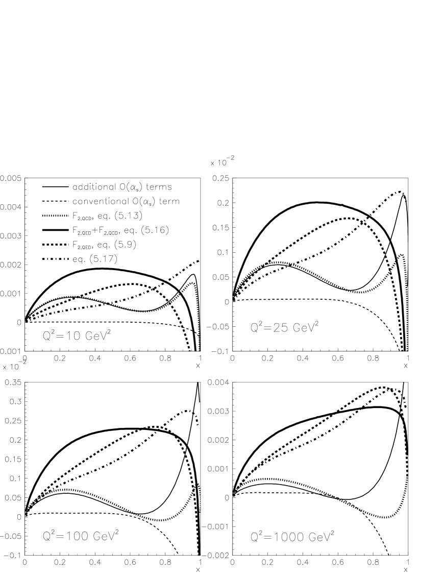
In Fig. 7 the sum of contributions to LO analysis of $F_{2}^{\gamma}$ coming from inclusion of $C_{\gamma}^{(1)},C_{q}^{(1)}$ and $k_{q}^{(1)}$ is compared to that given by the first term in (65), the purely QED contribution (42), the complete LO QCD contribution (46), as well as full QED$+$QCD expressions in my (49) and standard (50) approaches, in the latter including the contribution of $C_{\gamma}^{(0)}$ as well. In all calculations $M^{2}=Q^{2}$. The difference between the solid and dashโ€“dotted curves, which represent my and standard expressions for $F_{2,\mathrm{LO}}^{\gamma}$, is large and persists for all experimentally accessible values of $Q^{2}$. This is caused by the fact that in the whole kinematical region of $Q^{2}$ and for most of the region of $x$ accessible in current experiments, the sum of the three additional contributions included in the LO analysis proposed in this paper, is much larger than the contribution of the term generated by $P^{(0)}_{qq}$. But even for $x$ close to $x=1$ these additional terms are important as they help cancel in part the negative contribution of $C_{\gamma}^{(0)}$.

6.6 Dispensing with the DISฮณ factorization scheme

The quantitative comparison in Fig. 7 reveals another interesting difference: the term $\ln(1-x)$ in (17) is much less troubling within my formulation than within the standard one. The reason is simple: the contributions of additional terms compensate large part of the negative contribution of $C_{\gamma}^{(0)}$ at large $x$ and shifts the region where the complete LO expression turns negative much closer to $x=1$.

A simple explanation of the origins of this term is provided within the parton model derivation [4] of the expression (17) in which the parallel singularity associated with the splitting $\gamma\rightarrow q\overline{q}$ is regularized by means of quark masses and the troubling term $\ln(1-x)$ comes from the lower bound on the quark virtuality $\tau$ (see Fig. 1) in collinear kinematics

$$\tau_{\mathrm{min}}^{\mathrm{coll}}\equiv\frac{m_{q}^{2}}{1-x}\leq\tau\leq\tau_{\mathrm{max}}^{\mathrm{coll}}\equiv\frac{Q^{2}}{x}.$$ (70)

Performing the integration over $\tau$ in the limits $\tau_{\mathrm{min}}^{\mathrm{coll}}\leq\tau\leq M^{2}$, as prescribed by the definition (2) of PDF of the real photon, the primary QED splitting $\gamma\rightarrow q\overline{q}$ leads to [4]

$$f(x)\ln\left(\frac{M^{2}}{\tau_{\mathrm{min}}^{\mathrm{coll}}}\right)=f(x)\ln\left(\frac{M^{2}(1-x)}{m_{q}^{2}}\right)=f(x)\ln\left(\frac{M^{2}}{m_{q}^{2}}\right)+f(x)\ln(1-x),$$ (71)

where $f(x)=x^{2}+(1-x)^{2}$. Normally, the term proportional to $\ln(M^{2}/m_{q}^{2})$ is included in the quark distribution function $q(x,M)$, whereas the โ€œconstantโ€ part of (71), i.e. $f(x)\ln(1-x)$ goes into the coefficient function $C_{\gamma}^{(0)}$. Note that we cannot set $m_{q}=0$ in the logarithmic term. The complete expression for nonlogarithmic term of (17) includes, beside the term $f(x)\ln(1-x)$, also terms coming from the upper bound in (70) as well as from lower bound in integrals over the terms $m_{q}^{2}/\tau^{2}$, or 1/s1๐‘ 1/s. In these latter cases the dependence on $m_{q}$ enters $F_{2}^{\gamma}(x,Q^{2})$ through the multiplicative factor

$$c\equiv 1-\frac{\tau_{\mathrm{min}}^{\mathrm{coll}}}{M^{2}}=1-\frac{m_{q}^{2}}{M^{2}(1-x)},$$ (72)

where we can set $m_{q}=0$ in (72). Moreover, as the ratio $\tau_{\mathrm{min}}^{\mathrm{coll}}/M^{2}$ is formally of power correction type, we can neglect it even for $m_{q}>0$. The term $\ln(1-x)$ in $C^{(0)}_{\gamma}$ causes problems in phenomenological parameterizations primarily because it appears there decoupled from the value of the quark mass $m_{q}$ with which it originally entered the expression (70) for $\tau_{\mathrm{min}}$ and thus persists there even in the limit $m_{q}\rightarrow 0$, or when the quark mass is replaced by the initial scale $M_{0}$.

In the presence of the lower cuttโ€“off $M_{0}^{2}$ on the integration over the quark virtualities $\tau_{\mathrm{min}}^{\mathrm{coll}}$ in (70) should perhaps be replaced with $\tau_{0}\equiv\mathrm{max}(m_{q}^{2}/(1-x),M_{0}^{2})$. Sending $m_{q}\rightarrow 0$, but even for all realistic values of light quark masses and accessible $x$, we get $\tau_{0}=M_{0}^{2}$. This implies the replacement $\ln((1-x)/x)\rightarrow\ln(1/x)$ in $C_{\gamma}^{(0)}$, thereby removing most of the practical problems with the term $\ln(1-x)$ in (17).

Beside $\ln(1-x)$ there is another term in $C_{\gamma}^{(0)}$ that comes from nonzero quark mass, namely the last โ€œ+11+1โ€ in the nonlogarithmic part $8x(1-x)-1=8x(1-x)-2+1$. Discarding also this remaining trace of $m_{q}$ we get, setting $M^{2}=Q^{2}$,

$$C_{\gamma}^{(0)}(x,1)=\left[x^{2}+(1-x)^{2}\right]\ln\frac{1}{x}+8x(1-x)-2.$$ (73)

This expression is close to, but not identical QED formula for the constant part of $F_{2}^{\gamma}(x,Q^{2})$ obtained for massless quarks coupled photon with nonzero virtuality $P^{2}>0$ [24]

$$C_{\gamma}^{(0)}(x,1)=\left[x^{2}+(1-x)^{2}\right]\ln\frac{1}{x^{2}}+8x(1-x)-2.$$ (74)

The only difference between (73) and (74), i.e. the additional $1/x$ in the logarithm $\ln(1/x^{2})$ with respect to (73) reflects the fact that for $m_{q}=0$ and $P^{2}>0$ the lower bound $\tau_{\mathrm{min}}^{\mathrm{coll}}=xP^{2}$. The expression (73) for $C_{\gamma}^{(0)}$ is also close to that used for different reasons by Schuler and Sjรถstrand in their SaS1M and SaS2M parameterizations

$$C_{\gamma}^{(0)}(x,1)=\left[x^{2}+(1-x)^{2}\right]\ln\frac{1}{x}+6x(1-x)-1.$$ (75)

In Fig. 6 all three expressions (73-75) are compared to the standard one of eq. (17).

7 Conclusions

I have presented a reformulation of LO and NLO QCD analysis of $F_{2}^{\gamma}$, which separates genuine QCD effects from those due to pure QED and satisfies the basic requirement of factorization scale invariance. This reformulation differs substantially from the conventional LO and NLO analysis of $F_{2}^{\gamma}$.

Compared to the standard formulation at the LO it requires the inclusion of four additional terms, proportional to $C_{q}^{(1)},k_{q}^{(1)},C_{\gamma}^{(0)}$ and $C_{\gamma}^{(1)}$, all of which are known. Whereas in the standard approach the first three of them are part of the NLO approximation, the last one, i.e. the one proportional to $C_{\gamma}^{(1)}$, enters the standard formulation first at the NNLO. Detailed numerical analysis of the contributions of all these terms shows that in most of the kinematical region accessible experimentally their sum is much more important than the contribution of the term included in the standard LO expression for $F_{2}^{\gamma}$ and induced by $P_{qq}^{(0)}$. It is shown that in the reformulated LO QCD analysis of $F_{2}^{\gamma}$ the part of $C_{\gamma}^{(0)}$ proportional to $\ln(1-x)$, which in the standard formulation causes problems in the region $x\rightarrow 1$, is much less troubling. All the quantitative considerations were carried out for the pointlike part of $F_{2}^{\gamma}$ in the nonsinglet channel and under the simplifying assumption $\beta_{1}=0$. A realistic analysis of experimental data will necessitate the extension of the present formulation to the pointlike part of $F_{2}^{\gamma}$ in the singlet channel as well as the addition of the hadronic components in both channels. At the NLO a complete analysis requires the knowledge of two so far uncalculated quantities and is therefore currently impossible to perform.

Acknowledgments.
I thank W. van Neerven, E. Laenen and S. Larin for correspondence concerning higher order QCD calculations of photonic coefficient and splitting functions. I have enjoyed numerous discussion and correspondence on the subject of photon structure with J. Field and F. Kapusta who have advocated part of what I claim here for more than a decade.

References

  • [1] A. Vogt, in Procedings PHOTON โ€™97, Egmond aan Zee, May 1997, edt. F. Ernรฉ, World Scientific 1998
  • [2] S. Sรถldnerโ€“Rembold, in Procedings of XVIII International Symposium on Lepton-Photon Physics, Hamburg, 1997, hep-ex/9711005.
  • [3] R. Nisius, in Proceedings PHOTON โ€™99, Freiburg in Breisgau, May 1999, ed. S. Soeldnerโ€“Rembold, Nucl. Phys. Proc. Supp., in press
  • [4] J. Chรฝla, hep-ph/9811455
  • [5] J.H. Field, F. Kapusta, L. Poggioli, Phys. Lett. B 181, 362 (1986)
    J.H. Field, F. Kapusta, L. Poggioli, Z. Phys. C 36, 121 (1987)
    F. Kapusta, Z. Phys. C 42, 225 (1989)
  • [6] A. Vogt, in Proceedings PHOTON โ€™99, Freiburg in Breisgau, May 1999, ed. S. Soeldnerโ€“Rembold, Nucl. Phys. Proc. Supp., in press
  • [7] J. Chรฝla, M. Taลกevskรฝ, in Proceedings PHOTON โ€™99, Freiburg in Breisgau, May 1999, ed. S. Soeldnerโ€“Rembold, Nucl. Phys. Proc. Supp., in press, hep-ph/9906552
  • [8] J. Chรฝla, M. Taลกevskรฝ, in Proceedings of Workshop MC generators for HERA Physics, Hamburg 1999, p. 239, hep-ph/9905444
  • [9] P. Aurenche, J.-P. Guillet, M. Fontannaz, Z. Phys. C 64, 621 (1994)
  • [10] M. Glรผck, E. Reya, A. Vogt, Phys. Rev. D45, (1991), 3986
  • [11] H. D. Politzer, Nucl. Phys. B 194, 493 (1982)
  • [12] W. Bardeen, A. Buras, D. Duke and T. Muta, Phys. Rev D 18, 3998 (1978)
  • [13] J. Chรฝla, Z. Phys. C 43, 431 (1989)
  • [14] G. Curci, W. Furmanski, R. Petronzio, Nucl. Phys. B 175, 27 (1980)
  • [15] P. Aurenche, R. Baier, A. Douiri, M. Fontannaz, D. Schiff, Nucl. Phys. B 286, 553 (1987)
    P. Aurenche, R. Baier, M. Fontannaz, D. Schiff, Nucl. Phys. B 296, 661 (1987)
  • [16] G. Schuler, T. Sjรถstrand, Z. Phys. C 68, 607 (1995)
  • [17] E. Witten, Nucl. Phys. 120, 189 (1977)
  • [18] W. Bardeen, A. Buras, Phys. Rev. D 20, 166 (1979)
  • [19] J. Chรฝla, Phys. Lett. B 320, 186 (1994)
  • [20] M. Stratmann, Talk presented at the Workshop on Photon Interactions and the Photon Structure, Lund, 1998, hepโ€“ph/9811260
  • [21] E.B. Zijlstra and W.L. van Neerven, Phys. Lett. B 273, 476 (1991)
  • [22] E.B. Ziljstra and W.L. van Neerven, Nucl. Phys. B 383, 525 (1992)
  • [23] E. Laenen, S. Riemersma, J. Smith and W.L. van Neerven, Phys. Rev. D 49, 5753 (1994)
  • [24] A. Gorski, B.L. Ioffe, A. Yu. Khodjamirian, A. Oganesian, Z. Phys. C 44, 523 (1989)