Testing models with a nonminimal Higgs sector through the decay $t\to q+WZ$

Abstract

We study the contribution of the charged Higgs boson to the rare decay of the top quark $t\to q+WZ$ ($q=d,s,b$) in models with Higgs sectors that include doublets and triplets. Higgs doublets are needed to couple a charged Higgs with quarks, whereas the Higgs triplets are required to generate the nonstandard vertex $HWZ$ at the tree level. It is found that within a model that respects the custodial $SU(2)_{c}$ symmetry and avoids flavor–changing neutral current (FCNC) by imposing discrete symmetries, the decay mode $t\to b+WZ$ can reach a branching ratio (BR) of order $10^{-2}$, whereas the decay modes $t\to(d,\,s)+WZ$, can reach a similar BR in models where FCNC are suppressed by flavor symmetries.

INTRODUCTION

The mass of the top quark, which is larger than any other fermion mass in the standard model (SM) and almost as large as its scale of electroweak symmetry breaking (EWSB), cannot be explained within the SM [1]. This has originated speculations about the possible relationship between the top quark and the nature of the mechanism responsible for EWSB. Several models have been proposed, where such large mass can be accommodated or plays a significant role. In the supersymmetric (SUSY) extensions of the SM [2], the large value of the top quark mass can drive the radiative breaking of the electroweak symmetry; furthermore within the context of SUSY grand unified theories (GUT’s) the fermions of the third–family can be accommodated in scheemes where their masses arise from a single Yukawa term [3]. On the other hand, in some top–condensate (TC) models [4] it is postulated that new strong interactions bind the heavy top quark into a composite Higgs scenario.

From a more phenomenological point of view, it is also intriguing to notice that the top quark decay seems to be dominated by the SM mode ($t\to bW$), not only within the SM but also in theories beyond it, which makes the top quark decay width almost insensitive to the presence of new physics; unless the scale of new physics is lighter than the top quark mass itself, such that new states can appear in its decays. This is the case, for instance, in the general two Higgs doublet model (THDM–III) [5], where the flavor changing mode $t\to c+h$ can be important for a light Higgs boson ($h$), or in SUSY models with light stop quark and neutralinos, in whose case the decay $t\to\tilde{t}+\tilde{\chi^{0}}$ can also be relevant. But in general, the rare decays of the top quark have undetectable branching ratios (BR’s); for instance, the flavor–changing neutral current (FCNC) rare decays $t\to cV$ ($V=\gamma,Z,g$) have a very small BR in the SM, of the order $10^{-11}$ [6], and are out of reach of present and future colliders. A similar result is obtained in several extensions of the SM; for instance in the THDM–II, minimal SUSY extensions of the SM (MSSM) and left–right models, to mention some cases [7].

The rare decay $t\to qWZ$ $(q=b,s,d)$, may be above the threshold for the production of a real $WZ$ state, provided that $m_{t}\geq m_{q}+m_{W}+m_{Z}$. The possibilities to satisfy this relation depend on the final state $q$ and the precise value of the top quark mass, which according to the Particle Data Group [8] is $m_{t}=173.8\pm 5.2\,$ GeV. For the case when $q=b$, the top quark mass must satisfy $m_{t}\geq 176.1\pm 0.5$ GeV, where the uncertainty on the right–hand side is mostly due to the ambiguity in the bottom quark mass, thus $t\to bWZ$ can occur on–shell only if $m_{t}$ takes its upper allowed value (at $1\sigma$). However, if $q=d$ or $s$, the decays $t\to qWZ$ can occur even when $m_{t}$ takes its central value.

The value of BR($t\to bWZ$) predicted in SM is $5.4\times 10^{-7}$ [9], which is beyond the sensitivity of Tevatron Run II or even CERN Large Hadron Collider (LHC); thus its observation would truly imply the presence of new physics. For $q=d,s$ the SM result is even smaller, since the amplitude is supressed by the Cabibbo–Kobayashi–Maskawa (CKM) matrix elements $V_{tq}$. On the other hand, the decay mode $t\to qWZ$ can proceed through an intermediate charged Higgs boson that couples to both $tq$ and $WZ$ currents, and thus can be used to test the couplings of Higgs sectors beyond the SM [10].

The construction of extensions of the SM Higgs sector must satisfy the constraints impossed by the successful phenomenological relation $\rho\equiv m_{W}^{2}/m_{Z}^{2}\cos\theta_{w}=1$, which also measures the ratio between the neutral and charged current couplings strength. At tree level this relation is satisfied naturally in models that include only Higgs doublets, but in more general scenarios, there could be tree level contributions to $\rho-1$. Since the vertex $HWZ$ arises at tree level only for Higgs bosons lying in representations higher than the usual SM Higgs doublet, there could be violations of the constraints impossed by the $\rho$ parameter. However, tree–level deviations of the electroweak $\rho$ parameter from unity can be avoided by arranging the nondoublet fields and the vacuum expectation values (V.E.V’s) of their neutral members, so that a custodial $SU(2)_{c}$ symmetry is maintained [11]. On the other hand, a generic coupling of the charged Higgs boson with fermions may be associated with the possible appearence of FCNC in the Higgs–Yukawa sector. FCNC are automatically absent in the minimal SM with one Higgs doublet, however in multiscalar models large FCNC can appear if each quark flavor couples to more than one Higgs doublet [12]. FCNC can be avoided either by impossing some ad hoc discrete symmetry to the Yukawa Lagrangian, i.e., by coupling each type of fermion only to one Higgs doublet; or by using flavor symmetries. The former case is used in the so–called two Higgs doublet models I and II, whereas the last one is associated with model III, here FCNC is only suppressed by some ansatz for the Yukawa matrices, for instance the Li–Sher one: $(Y_{q})_{ij}=\sqrt{m_{i}m_{j}}/m_{W}$, whose phenomenology was studied in [13, 14].

In this Rapid Communication we shall consider, in a very general setting, the contribution of a charged Higgs boson to the decay $t\to qWZ$, and present the results in terms of two factors that parametrize the doublet–triplet mixing and the nonminimal Yukawa couplings, respectively. Then, we discuss the values that these parameters can take for specific extensions of the SM, when the constraints from both the custodial symmetry and FCNC are satisfied, and present the predicted values for BR($t\to qWZ$).

The decay $t\to qWZ$

We are interested in studying the contribution of charged Higgs boson to the rare decay of the top quark $t\to qWZ$ ($q=d,s,b$), within the context of models with extended Higgs sector that include additional Higgs doublets and triplets. The charged Higgs will be assumed to be the lightest charged mass eigenstate that results from the general mixing of doublets and triplets in the charged sector.

Higgs doublets are needed in order to couple the charged Higgs with quarks; the vertex $tqH^{\pm}$ will be written as follows

$$\frac{ig}{2\sqrt{2}m_{W}}\eta_{tq}\cos\alpha\left[(m_{t}\cot\beta+m_{q}\tan\beta)+(m_{t}\cot\beta-m_{q}\tan\beta)\gamma_{5}\right],$$ (1)

which can be considered as a modification of the result obtained for the Yukawa sector of the general THDM, where $\cos\alpha$ is included to account for the doblet–triplet mixing; $\tan\beta$ is the ratio of the V.E.V.’s of the two scalar doublets. The charged Higgs coupling to the quarks is also determined by the parameters $\eta_{tq}$, which is equal to the CKM mixing matrix only for model–II, i.e., $\eta_{tq}^{II}=V_{tq}$; however, in the general case (THDM–III), one can have $\eta_{tq}^{III}>V_{tq}$ [5].

On the other hand, we require a representation higher than the doublet, in order to obtain a sizeable coupling $HWZ$ at tree level, which is written as

$$-\frac{igm_{W}}{\cos\theta_{w}}\sin\alpha g_{\mu\nu}.$$ (2)

In order to evaluate the decay $t\to qWZ$, we shall write a general amplitude to describe the contribution of the intermediate charged Higgs, neglecting the SM contribution, which is a good approximation since the corresponding BR is very suppressed. To calculate the amplitude one also needs to take into account the finite width of the intermediate charged Higgs boson with momentum $p_{H}$, mass $m_{H}$, and width $\Gamma_{H}$, for this we shall use the relativistic Breit–Wigner form of the propagator in the unitary gauge. Then, the amplitude can be written in general as

$${\cal M}=A\left[\overline{u}(p_{q})(a+b\gamma_{5})u(p_{t})\right]\left(\frac{-i}{p_{H}^{2}-\hat{m}_{H}^{2}}\right)\left[g_{\mu\nu}\epsilon_{W}^{*\mu}\epsilon_{Z}^{*\nu}\right],$$ (3)

where $\hat{m}_{H}\equiv m_{H}+(i/2)\Gamma_{H}$; $a$, $b$, and $A$ are constants related to the parameters $\alpha$ and $\eta_{tq}$ previously mentioned

$$a = m_{t}\cot\beta+m_{q}\tan\beta,$$ (4)

$$b = m_{t}\cot\beta-m_{q}\tan\beta,$$ (5)

$$A = \frac{g^{2}}{2\sqrt{2}\cos\theta_{w}}\eta_{tq}\cos\alpha\sin\alpha.$$ (6)

To calculate the partial decay width, we shall perform a numerical integration of the expression for the squared amplitude, over the standard three–body phase space, namely

$$\Gamma(t\to qWZ)=\frac{1}{(2\pi)^{3}}\frac{1}{32m_{t}^{3}}\int\mid\overline{{\cal M}}\mid^{2}ds\,dt.$$ (7)

$\mid\overline{{\cal M}}\mid^{2}$ denotes the squared amplitude, averaged over initial spins and summed over final polarizations, it has the form

$$\mid\overline{{\cal M}}\mid^{2}=\frac{\mid A\mid^{2}[(a^{2}+b^{2})(m_{t}^{2}+m_{q}^{2}-s)+(a^{2}-b^{2})2m_{t}m_{q}]}{(s-m_{H}^{2})^{2}+m_{H}^{2}\Gamma_{H}^{2}}\left[2+\left(\frac{s-m_{W}^{2}-m_{Z}^{2}}{2m_{W}m_{Z}}\right)^{2}\right].$$ (8)

The integration limits are

$$(m_{W}+m_{Z})^{2}\leq s\leq(m_{t}-m_{q})^{2},$$ (9)

and

$$t^{-}\leq t\leq t^{+},$$ (10)

where

$$t^{\pm}=m_{t}^{2}+m_{Z}^{2}-\frac{1}{2s}[(s+m_{t}^{2}-m_{q}^{2})(s+m_{Z}^{2}-m_{W}^{2})\mp\lambda^{1/2}(s,m_{t}^{2},m_{q}^{2})\lambda^{1/2}(s,m_{Z}^{2},m_{W}^{2})],$$ (11)

and $\lambda(x,y,z)=(x+y-z)^{2}-4xy$.

The branching ratio for this decay is obtained as the ratio of Eq. (7) to the total width of the top quark, which will include the modes $t\to qW$ and $t\to qH$; the expressions for the widths are

$$\Gamma(t\to qW^{+})=\frac{G_{F}m_{t}^{3}}{8\pi\sqrt{2}}V_{tq}\left(1-\frac{m_{W}^{2}}{m_{t}^{2}}\right)^{2}\left(1+2\frac{m_{W}^{2}}{m_{t}^{2}}\right)\left[1-\frac{2\alpha_{s}}{3\pi}\left(\frac{2\pi^{2}}{3}-\frac{5}{2}\right)\right],$$ (12)

and

$$\Gamma(t\to qH^{+}) = \frac{g^{2}}{128\pi m_{W}^{2}m_{t}}\eta_{tq}\cos^{2}\alpha\left[a^{2}[(m_{t}+m_{q})^{2}-m_{H}^{2}]+b^{2}[(m_{t}-m_{q})^{2}-m_{H}^{2}]\right]$$ (13)

$$\times \lambda^{1/2}\left(1,\frac{m_{q}^{2}}{m_{t}^{2}},\frac{m_{H}^{2}}{m_{t}^{2}}\right).$$ (14)

On the other hand, the Higgs width will include the fermionic decays into $H\to c\overline{s}$ and $H\to\tau\nu_{\tau}$; adding them we obtain

$$\Gamma(H^{+}\to f\overline{f^{\prime}})=\frac{g^{2}m_{H}}{32\pi m_{W}^{2}}\cos^{2}\alpha\left[3\eta_{cs}(m_{c}^{2}\cot^{2}\beta+m_{s}^{2}\tan^{2}\beta)+m_{\tau}^{2}\tan^{2}\beta\right]$$ (15)

as well as the bosonic mode $H\to WZ$

$$\Gamma(H^{+}\to W^{+}Z) = \frac{g^{2}m_{H}}{64\pi}\sin^{2}\alpha\left[1+\left(\frac{m_{W}^{2}}{m_{H}^{2}}\right)^{2}+\left(\frac{m_{Z}^{2}}{m_{H}^{2}}\right)^{2}-2\frac{m_{W}^{2}}{m_{H}^{2}}-2\frac{m_{Z}^{2}}{m_{H}^{2}}+10\frac{m_{W}^{2}}{m_{H}^{2}}\frac{m_{Z}^{2}}{m_{H}^{2}}\right]$$ (16)

$$\times \lambda^{1/2}\left(\frac{m_{H}^{2}}{m_{W}^{2}},\frac{1}{\cos^{2}\theta_{w}},1\right).$$ (17)

Results and conclusions

In order to present the results for the mode $t\to bWZ$, i.e., $q=b$, we shall assume that the top quark mass takes its upper allowed value, and will consider a Yukawa sector similar to the model–II, in whose case the factor $\eta_{tb}$ is equal to the CKM matrix element $V_{tb}$ $(\simeq 1)$; the results are shown for two values of $\tan\beta$ (2, and $m_{t}/m_{b}$) which are acceptable for GUT–Yukawa unification. For the factor $\cos\alpha\sin\alpha$, which is part of the constant $A$, we shall consider first the value $\frac{1}{2}$, which corresponds to the maximum value that can be expected to arise in an scenario where the custodial symmetry is respected, for instance in a model with one Higgs doublet and two Higgs triplets of hypercharges 0 and 2, respectively, where one can align the V.E.V.’s to respect the custodial symmetry and obtaining $\rho=1$[11]. On the other hand, to consider a model without a custodial symmetry, we take the value $\sin\alpha=0.04$, which corresponds to the maximum value that is allowed by the experimental error in the $\rho$ parameter [15]. With all these considerations, we shown in Fig. 2 our results for the BR of the decay $t\to bWZ$; we notice that it can reach a maximum value of order $1.78\times 10^{-2}$.

For the decays into the light quarks, still working within the framework of model II, we obtain a very suppressed result, where we are taking now the central value for the top quark mass, namely, for $t\to sWZ$ we get a maximum value for the BR of order $1.95\times 10^{-6}$ for $\sin\alpha\cos\alpha=\frac{1}{2}$ and $\tan\beta=2$; for $t\to dWZ$ we get results even smaller and thus uninteresting. On the other hand, if we consider a model with a Yukawa sector of the type THDM–III, the coupling of the charged Higgs with the quarks is not determined by the CKM mixing matrix, then the couplings $t\bar{d}H^{-}$ and $t\bar{s}H^{-}$ may not be suppresed. Although in model III there can be dangerous FCNC, it happens that such effects have not been tested by top quark decays, and thus can give large and detectable effects [14]. For the parameter $\alpha$ we take the same values of the previous case, assuming also $\eta_{ts}=\eta_{td}$ we get a maximum value for the BR of order $1.31\times 10^{-3}$ for both $t\to(d,\,s)+WZ$, as shown in Fig. 2.

We conclude from our results that there exist a region of parameters where it is possible to obtain a large BR for the decay $t\to bWZ$. Moreover, for $m_{H}=162$ to $m_{H}=182$ GeV, $\cos\alpha\sin\alpha=\frac{1}{2}$, and $\tan\beta=m_{t}/m_{b}$ we obtain a BR larger than the one predicted by the SM. Furthermore, the maximum value for the BR, of order $10^{-2}$, seems factible to be detected at the future CERN LHC, where about $10^{8}$ top quark pairs could be produced, and one would have $10^{6}$ events of interest with only one top quark decaying rarely. If we also include the decays of the W and Z into leptonic modes, to allow a clear signal, one would end with about $1.3\times 10^{4}$ events, which is interesting enough to perform a future detailed study of backgrounds; however this is beyond the scope of present work. On the other hand, we observe from Fig. 2 that even within models without a custodial symmetry with $\sin\alpha=0.04$, it is possible to get BR for the decay $t\to sWZ$ larger than the SM result, or the result obtained within models where $\sin\alpha\cos\alpha=\frac{1}{2}$, depending on the value of $\tan\beta$; in some cases it can reach a BR of order $1.31\times 10^{-3}$.

In conclusion, we find that the decay $t\to qWZ$ is sensitive to the contribution of new physics, in particular from a charged Higgs boson, which makes this mode an interesting arena for testing physics beyond the SM.

FIG. 1.: Branching ratio for the decay $t\to bWZ$, as a function of $m_{H}$ for $\cos\alpha\sin\alpha=\frac{1}{2}$ (upper curves) and $\sin\alpha=0.04$ (lower curves); and for $\tan\beta=\frac{m_{t}}{m_{b}}$ (solid curves) and $\tan\beta=2$ (dashed curves); it is also assumed that $\eta_{tq}=V_{tq}$. The line indicate the SM prediction.

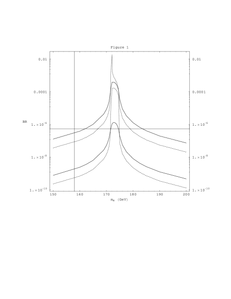
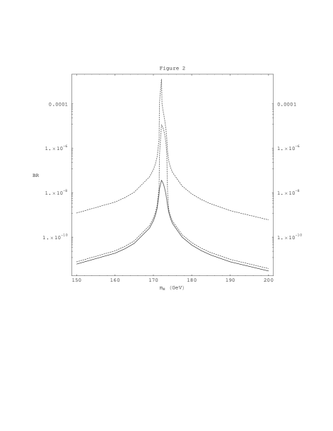
FIG. 2.: Branching ratio for the decay $t\to sWZ$, as a function of $m_{H}$ for $\cos\alpha\sin\alpha=\frac{1}{2}$ (upper dashed and solid curve) and $\sin\alpha=0.04$ (middle curve); and for $\tan\beta=\frac{m_{t}}{m_{b}}$ (solid curve) and $\tan\beta=2$ (dashed curves); taking also $\eta_{tq}=1$.

- [1] W. Hollik, Radiative Corrections: Applications of Quantum Field Theory to Phenomenology, Proceedings Edited by Joan Sòla, Singapore, World Scientific, (1999) p. 44.
- [2] H. P. Nilles, Phys. Rep. 110, 1 (1984); H. Haber and G. L. Kane, ibid. 117, 75 (1985).
- [3] H. Arason et al., Phys. Rev. Lett. 67, 2933 (1991); A. Giveon, L. J. Hall, and U. Sarid, Phys. Lett. B 271, 138 (1991).
- [4] W. A. Bardeen, C. T. Hill, and M. Lindner, Phys. Rev. D 41, 1647 (1990).
- [5] T. Cheng and M. Sher, Phys. Rev. D 35, 3484 (1987); M. Sher and Y. Yuan, ibid. 44, 1461 (1991); J. L. Díaz Cruz and G. Lopez Castro, Phys. Lett. B 301, 405 (1993).
- [6] J. L. Díaz Cruz et al., Phys. Rev. D 41, 891 (1990).
- [7] See for instance: G. Eilam, J. L. Hewett, and A. Soni, Phys. Rev. D 44, 1473 (1991).
- [8] Particle Data Group, C. Caso et al., Eur. Phys. J. C 3, 1 (1998).
- [9] R. Decker, M. Nowakowski,and A. Pilaftsis, Z. Phys. C 57, 339 (1993); G. Mahlon and S. Parke, Phys. Lett. B 347, 394 (1995); E. Jenkins, Phys. Rev. D 56, 458 (1997); G. Mahlon, “Theoretical Expectations in Radiative Top Decays”, talk given at the Physics at Run II: Workshop on Top Physics, Batavia, IL, (1998).
- [10] T. G. Rizzo, Phys. Rev. D 41, 1504 (1990); K. Cheung, R. J. N. Phillips, and A. Pilaftsis, ibid. 51, 4731 (1995); D. A. López Falcón and J. L. Díaz Cruz, AIP Conf. Proc. 490, 374 (1999).
- [11] For a detailed discussion of models with Higgs triplets, see J. F. Gunion, R. Vega, and J. Wudka , Phys. Rev. D 42, 1673 (1990).
- [12] J. F. Gunion, H. E. Haber, G. Kane, and S. Dawson. The Higgs Hunter’s Guide, (Addison–Wesley, Reading, MA, 1990), Chap 4, p. 203.
- [13] J. L. Díaz Cruz, J. J. Godina, and G. López Castro, Phys. Rev. D 51, 5263 (1995); D. Atwood, L. Reina, and A. Soni, ibid. 55, 3156 (1997).
- [14] J. L. Díaz Cruz et al., Phys. Rev. D 60, 11 5014 (1999).
- [15] T. G. Rizzo, Mod. Phys. Lett. A 6, 1961 (1991).