Abstract

PACS 12.15.Mm,12.60.-i, 14.65.Ha, 14.70.-e

PACS 12.15.Mm,12.60.-i, 14.65.Ha, 14.70.-e

1 Introduction

The mixing among light quarks $u,d,s,c,b$ is precisely measured and in agreement with the Standard Model (SM)  [1]. In contrast the gauge couplings of the top quark are poorly known experimentally. However, its mixing is strongly constrained in the SM. In particular, the Glashow-Iliopoulos-Maiani (GIM) mechanism  [2] forbids all tree-level flavour-changing neutral currents. On the other hand the top mixing can be large in simple SM extensions. It is then important to measure (bound) it because any positive signal will stand for new physics.

The top flavour-changing neutral couplings (FCNC) with a light quark $q=u,c$ and a $Z$ boson, a photon $A$ or a gluon $G^{a}$ are conveniently parametrized by the Lagrangian  [3]

$${\cal L} = -\frac{g}{2c_{W}}\bar{t}\gamma^{\mu}\left(X^{L}_{tq}P_{L}+X^{R}_{tq}P_{R}\right)qZ_{\mu}$$

$$-\frac{g}{2c_{W}}\bar{t}\left(\kappa_{tq}^{(1)}-i\kappa_{tq}^{(2)}\gamma_{5}\right)\frac{i\sigma^{\mu\nu}q_{\nu}}{m_{t}}qZ_{\mu}$$

$$-e\bar{t}\left(\lambda_{tq}^{(1)}-i\lambda_{tq}^{(2)}\gamma_{5}\right)\frac{i\sigma^{\mu\nu}q_{\nu}}{m_{t}}qA_{\mu}$$

$$-g_{s}\bar{t}\left(\zeta_{tq}^{(1)}-i\zeta_{tq}^{(2)}\gamma_{5}\right)\frac{i\sigma^{\mu\nu}q_{\nu}}{m_{t}}T^{a}qG^{a}_{\mu}+{\rm h.c.},$$

where $P_{L,R}=\frac{1\mp\gamma_{5}}{2}$ and $T^{a}$ are the Gell-Mann matrices normalized to fulfil ${\rm Tr}(T^{a}T^{b})=\frac{\delta^{ab}}{2}$. These vertices are constrained by the data collected at the Fermilab Tevatron  [4]

$$\begin{array}[]{rcl}X_{tq}&\equiv&\sqrt{|X^{L}_{tq}|^{2}+|X^{R}_{tq}|^{2}}\leq 0.84,\\ \kappa_{tq}&\equiv&\sqrt{|\kappa^{(1)}_{tq}|^{2}+|\kappa^{(2)}_{tq}|^{2}}\leq 0.78,\\ \lambda_{tq}&\equiv&\sqrt{|\lambda^{(1)}_{tq}|^{2}+|\lambda^{(2)}_{tq}|^{2}}\leq 0.26,\\ \zeta_{tq}&\equiv&\sqrt{|\zeta^{(1)}_{tq}|^{2}+|\zeta^{(2)}_{tq}|^{2}}\leq 0.15.\end{array}$$ (2)

At this point one can make three obvious questions:

• How large can these couplings be when all experimental data are taken into account ?

• Do simple models exist saturating the resulting limits ?

• How precisely will future colliders measure these vertices ?

We will address these three questions in turn. First we review the limits on the mixing between light and heavy quarks in Section 2, paying special attention to the $t$ couplings. Then in Section 3 we argue that the top mixing can be large in the simplest SM extensions with vector-like quarks. Finally we discuss the precision with which these couplings will be measured at future hadron colliders in Section 4. Section 5 is devoted to conclusions. For an extended analysis see Ref.  [5].

2 Experimental limits on quark mixing

Eq. (1) is a piece of a general effective Lagrangian of which the SM is the lowest order part  [3]. All terms in $\cal L$ result from dimension six operators after spontaneous symmetry breaking. But it can be argued that having different origin the size of their coupling constants can be quite different. The $\gamma^{\mu}$ terms are dimension four and we expect them to be larger than the $\sigma^{\mu\nu}$ terms which are dimension five. This is what happens in the models we study in next Section. However, when dealing with future limits at large colliders in Section 4, we must investigate all possible scenarios and then allow for arbitrary $\sigma^{\mu\nu}$ couplings within existing experimental bounds. In the rest of this Section we discuss the limits on dimension four (renormalizable) couplings. We include charged currents because as in the SM, charged (${\cal L}_{W}$) and neutral (${\cal L}_{Z}$) currents are related in SM extensions with vector-like fermions.

2.1 Direct limits

The $W$ couplings $V_{qq^{\prime}}$ in

$${\cal L}_{W}=-\frac{g}{2\sqrt{2}}\bar{q}_{L}V_{qq^{\prime}}\gamma^{\mu}q^{\prime}_{L}W^{+}_{\mu}+{\rm h.c.},$$ (3)

where the sum over $q$ and $q^{\prime}$ is understood, are consistent with a $3\times 3$ unitary Cabbibo-Kobayashi-Maskawa  [6] (CKM) matrix  [7],

$$\begin{array}[]{lll}|V_{ud}|=0.9740\pm 0.0010,&|V_{us}|=0.2196\pm 0.0023,&|V_{ub}|=0.0033\pm 0.0008,\cr|V_{cd}|=0.224\pm 0.016,&|V_{cs}|=1.04\pm 0.16,&|V_{cb}|=0.0395\pm 0.0017.\end{array}$$ (4)

While the $Z$ couplings $c^{L,R}_{qq^{\prime}}$ in

$${\cal L}_{Z}=-\frac{g}{2c_{W}}\left(\bar{q}_{L}c^{L}_{qq^{\prime}}\gamma^{\mu}q^{\prime}_{L}+\bar{q}_{R}c^{R}_{qq^{\prime}}\gamma^{\mu}q^{\prime}_{R}\right)Z_{\mu},$$ (5)

where $c^{L,R}_{tq}$ are equal to $X^{L,R}_{tq}$ in Eq. (1), are diagonal and universal within experimental errors  [7, 8, 9],

$$\begin{array}[]{lll}|c^{L,R}_{uc}|\leq 1.2\times 10^{-3},&&\cr|c^{L,R}_{ds}|\leq 4.1\times 10^{-5},&|c^{L,R}_{db}|\leq 1.1\times 10^{-3},&|c^{L,R}_{sb}|\leq 1.9\times 10^{-3},\end{array}$$ (6)

$$\begin{array}[]{ll}c^{L}_{uu}=0.656\pm 0.032,&c^{L}_{cc}=0.690\pm 0.013,\cr c^{R}_{uu}=-0.358\pm 0.026,&c^{R}_{cc}=-0.321\pm 0.019,\cr c^{L}_{dd}=-0.880\pm 0.022,&c^{L}_{bb}=-0.840\pm 0.005,\cr c^{R}_{dd}=-0.054^{+0.154}_{-0.096},&c^{R}_{bb}=0.194\pm 0.018.\end{array}$$ (7)

The diagonal $u$ and $d$ couplings are measured in atomic parity violation and in the SLAC polarized-electron experiments and the $c$ and $b$ couplings result from a fit to precise electroweak data at the $Z$ peak  [10]. The sign of the right-handed (RH) couplings is fixed by the corresponding off-peak asymmetries. On the other hand the $s$ couplings are less precisely measured but also consistent with the SM fermion assignments. The off-diagonal couplings in Eq. (6) vanish in the SM as a consequence of the GIM mechanism  [2]. Whereas the diagonal couplings in Eq. (7) are a function of a unique angle

$$c^{L,R}_{qq}=2\left(T^{L,R}_{3q}-Q_{q}\sin^{2}\theta_{W}\right),$$ (8)

where $T^{L,R}_{3q}$ and $Q_{q}$ are the quark isospin and electric charge and $\theta_{W}$ the electroweak mixing angle. All data in Eqs. (4,6,7) agree with the SM within experimental errors, but what do we know about the top quark ?

At Fermilab Tevatron it has been established that  [11]

$$\frac{|V_{tb}|^{2}}{|V_{td}|^{2}+|V_{ts}|^{2}+|V_{tb}|^{2}}=0.99\pm 0.29,$$ (9)

however, although consistent with the unitarity of the $3\times 3$ CKM matrix, this ratio tells little about it. On the other hand (Eq. (2))

$$|c^{L,R}_{tq}|=|X^{L,R}_{tq}|\leq 0.84,$$ (10)

if $t$ mainly decays as in the SM. LEP2 data give a similar limit  [12]. Thus, the direct bounds on top mixing, Eqs. (9,10), are somewhat weak, leaving room for large new effects near the electroweak scale.

2.2 Indirect limits

One must also wonder about indirect constraints on quark mixing, although they are model dependent. Let us revise the estimates discussed in Ref.  [13] for illustration. Assuming only one non-zero FCNC $c^{L}_{tc}$ in Eq. (5) and integrating the heavy top quark the following effective Lagrangian for the left-handed (LH) down quarks is generated:

$${\cal L}^{eff}_{Z}=-\frac{g}{2c_{W}}\frac{m_{t}^{2}}{v^{2}}\frac{1}{16\pi^{2}}ln\frac{\Lambda^{2}}{m_{t}^{2}}\left(V_{cj}^{*}c^{L}_{ct}V_{ti}+V_{tj}^{*}c^{L}_{tc}V_{ci}\right)\bar{q}_{Lj}\gamma^{\mu}q_{Li}Z_{\mu}+{\rm h.c.},$$ (11)

where $\Lambda$ is a cut-off integral and $v$ the electroweak vacuum expectation value $\sim 250\ {\rm GeV}$. Then bounds on $c^{L}_{tc}$ can be derived comparing with neutral meson mass differences and rare decays. However, although with a minimal set of assumptions, this calculation is too rough and the corresponding indirect constraints too stringent. Whatever new physics is beyond the SM is unlikely that the net effect is only one non-zero FCNC. In general there will be more heavy degrees of freedom which after integrating them out will generate new effective contributions cancelling partially ${\cal L}^{eff}_{Z}$ in Eq. (11). This is the case, for instance, in the simplest SM extension with a new quark isosinglet $T$ of charge $\frac{2}{3}$. As discussed in next Section the $V_{cj}^{*}c^{L}_{ct}V_{ti}+V_{tj}^{*}c^{L}_{tc}V_{ci}$ coupling in Eq. (11) must be replaced (up to diagonal terms) by $V_{\alpha j}^{*}X_{\alpha\beta}^{L}V_{\beta i}$, where $\alpha,\beta$ run over all quarks of charge $\frac{2}{3}$ and $X_{tc}^{L}=c^{L}_{tc}$. As $X_{\alpha\beta}^{L}=V_{\alpha m}V_{\beta m}^{*}$, where $m=d,s,b$ is summed up, then

$$V_{\alpha j}^{*}X_{\alpha\beta}^{L}V_{\beta i}=V_{\alpha j}^{*}V_{\alpha m}V_{\beta m}^{*}V_{\beta i}=\delta_{jm}\delta_{mi}=\delta_{ji},$$ (12)

implying no FCNC in the down sector if the up quarks are degenerate. When the actual couplings and masses are introduced, the cancellation is not complete. If $T$ is very heavy, it decouples and $t$ does not have large FCNC.

The constraints on RH FCNC appear to be weaker due to the absence of RH charged currents in the SM. Still similar comments apply. If only one RH coupling $c^{R}_{tc}$ in Eq. (5) does not vanish, the $\rho$ parameter through the $Z$ boson self-energy bounds its size. Again in definite models this restriction is smoothed. If the SM is extended with a new heavy quark isodoublet $\left(\begin{array}[]{c}T\\ B\end{array}\right)$ of charges $\left(\begin{array}[]{c}\frac{2}{3}\\ -\frac{1}{3}\end{array}\right)$, the $T$ and $B$ contributions to the $\rho$ parameter cancel if the quarks are degenerate. If the top mixing is non-negligible the cancellation is not complete.

In summary, indirect constraints restrict FCNC but their application must be done in a model dependent basis. In fact in the two SM extensions just mentioned the top FCNC can be large but without saturating the direct bounds in Eq. (10). For example  [9]:

$$\begin{array}[]{ll}|c^{L}_{tc}|=|X^{L}_{tc}|\leq 0.082,&{\rm for\ an\ extra\ quark\ isosinglet}\ T,\\ |c^{R}_{tc}|=|X^{R}_{tc}|\leq 0.16,&{\rm for\ an\ extra\ quark\ isodoublet}\ \left(\begin{array}[]{c}T\\ B\end{array}\right).\end{array}$$ (13)

The mixing with the $u$ quark can be almost as large as with the $c$ quark but the top can not have a large mixing with both at the same time. Otherwise, it would be also a large coupling between $u$ and $c$, what is experimentally excluded (Eq. (6)).

3 Simple SM extensions with large top mixing

Let us discuss in more detail the two simplest SM extensions with vector-like quarks allowing for a large top mixing with the up or charm quark.

3.1 One extra isosinglet

The charged and neutral current terms in the Lagrangian read (in the current eigenstate basis)

$${\cal L}_{W}=-\frac{g}{2\sqrt{2}}\bar{u}_{Li}^{0}\gamma^{\mu}d_{Li}^{0}W^{+}_{\mu}+{\rm h.c.}$$ (14)

and

$${\cal L}_{Z}=-\frac{g}{2c_{W}}\left(\bar{u}_{Li}^{0}\gamma^{\mu}u_{Li}^{0}-\bar{d}_{Li}^{0}\gamma^{\mu}d_{Li}^{0}-2s_{W}^{2}J^{\mu}_{EM}\right)Z_{\mu},$$ (15)

respectively. $i=1,2,3$ are the three standard families. Diagonalizing the fermion mass matrices, the current eigenstates can be written as linear combinations of the mass eigenstates

$$u_{Li}^{0}=U^{uL}_{i\alpha}u_{L\alpha},\ \ d_{Li}^{0}=U^{dL}_{ij}d_{Lj}.$$ (16)

Greek (Latin) indices run always from 1 to 4 (3). Then

$${\cal L}_{W}=-\frac{g}{2\sqrt{2}}\bar{u}_{L\alpha}V_{\alpha i}\gamma^{\mu}d_{Li}W^{+}_{\mu}+{\rm h.c.}$$ (17)

and

$${\cal L}_{Z}=-\frac{g}{2c_{W}}\left(\bar{u}_{L\alpha}X^{uL}_{\alpha\beta}\gamma^{\mu}u_{L\beta}-\bar{d}_{Li}\gamma^{\mu}d_{Li}-2s_{W}^{2}J^{\mu}_{EM}\right)Z_{\mu},$$ (18)

with

$$V_{\alpha j}=U^{uL*}_{i\alpha}U^{dL}_{ij}$$ (19)

and

$$X^{uL}_{\alpha\beta}=U^{uL*}_{m\alpha}U^{uL}_{m\beta}=V_{\alpha m}V^{*}_{\beta m}=\delta_{\alpha\beta}-U^{uL*}_{T^{0}\alpha}U^{uL}_{T^{0}\beta}\ ,$$ (20)

as announced in Section 2 and used in Eq. (12). (Note that we have introduced a superscript to distinguish up, $u$, and down, $d$, mixing matrices. We omit it when the indices specify the quark flavour, as for instance in Eq. (1).) This type of models have been studied by many authors  [8, 9, 14]. The important point here is: how large can the top mixing be ? $U^{uL}_{T^{0}\alpha}$ parametrizes the departure from the SM. The constraints on $V_{qq^{\prime}}$ and $c^{L,R}_{qq^{\prime}}=\pm X^{L,R}_{qq^{\prime}}-2\delta_{qq^{\prime}}Q_{q}\sin^{2}\theta_{W}$ (where the $+(-)$ sign is for the up (down) quarks) from present data (Eqs. (4,6,7)) translate into ($s^{(^{\prime})},c^{(^{\prime})}$ stand for sinus and cosinus of the corresponding mixing angle)

$$U^{uL}_{T^{0}\alpha}=\left(0\ \ ss^{\prime}\ \ sc^{\prime}\ \ c\right),$$ (21)

where the up entry is much smaller to maximize the top mixing with the charm quark $X^{L}_{tc}=-s^{2}s^{\prime}c^{\prime}$ in Eq. (20), obtaining $|X^{L}_{tc}|\leq 0.082$  [9]. If we want to maximize the top mixing with the up quark, the rôle of the charm and the up is reversed in Eq. (21), and $|X^{L}_{tu}|\leq 0.047$. The indirect constraints are also fulfilled.

3.2 One extra isodoublet

In this model there are RH charged currents and RH FCNC which can be large. With an extra quark isodoublet $\left(\begin{array}[]{c}T^{0}\\ B^{0}\end{array}\right)$ the charged and neutral current terms in the Lagrangian read ($u^{0}_{L4}$ ($d^{0}_{L4}$) corresponds to $T^{0}_{L}$ ($B^{0}_{L}$))

$${\cal L}_{W}=-\frac{g}{2\sqrt{2}}\left(\bar{u}_{L\alpha}^{0}\gamma^{\mu}d_{L\alpha}^{0}+\bar{T}_{R}^{0}\gamma^{\mu}B_{R}^{0}\right)W^{+}_{\mu}+{\rm h.c.}$$ (22)

and

$${\cal L}_{Z} = -\frac{g}{2c_{W}}(\ \bar{u}_{L\alpha}^{0}\gamma^{\mu}u_{L\alpha}^{0}+\bar{T}_{R}^{0}\gamma^{\mu}T_{R}^{0}-\bar{d}_{L\alpha}^{0}\gamma^{\mu}d_{L\alpha}^{0}$$ (23)

$$-\bar{B}_{R}^{0}\gamma^{\mu}B_{R}^{0}-2s_{W}^{2}J^{\mu}_{EM}\ )\ Z_{\mu},$$

in the current eigenstate basis, and

$${\cal L}_{W}=-\frac{g}{2\sqrt{2}}\left(\bar{u}_{L\alpha}V^{L}_{\alpha\beta}\gamma^{\mu}d_{L\beta}+\bar{u}_{R\alpha}V^{R}_{\alpha\beta}\gamma^{\mu}d_{R\beta}\right)W^{+}_{\mu}+{\rm h.c.}$$ (24)

and

$${\cal L}_{Z} = -\frac{g}{2c_{W}}(\ \bar{u}_{L\alpha}\gamma^{\mu}u_{L\alpha}+\bar{u}_{R\alpha}X^{uR}_{\alpha\beta}\gamma^{\mu}u_{L\beta}-\bar{d}_{L\alpha}\gamma^{\mu}d_{L\alpha}$$ (25)

$$-\bar{d}_{R\alpha}X^{dR}_{\alpha\beta}\gamma^{\mu}d_{R\beta}-2s_{W}^{2}J^{\mu}_{EM}\ )\ Z_{\mu},$$

in the mass eigenstate one. The generalized CKM matrices are written

$$V^{L}_{\alpha\beta}=U^{uL*}_{\rho\alpha}U^{dL}_{\rho\beta},\ \ V^{R}_{\alpha\beta}=U^{uR*}_{T^{0}\alpha}U^{dR}_{B^{0}\beta}$$ (26)

and the neutral couplings

$$X^{uR}_{\alpha\beta}=U^{uR*}_{T^{0}\alpha}U^{uR}_{T^{0}\beta},\ \ X^{dR}_{\alpha\beta}=U^{dR*}_{B^{0}\alpha}U^{dR}_{B^{0}\beta},$$ (27)

where the unitary matrices $U^{L(R)}$ diagonalize the quark mass matrices. A similar analysis as for the isosinglet gives

$$U^{uR}_{T^{0}\alpha}=\left(0\ \ s\ \ c\ \ 0\right),\ \ U^{uR}_{B^{0}\alpha}=\left(0\ \ \epsilon\ \ 0\ \ \sqrt{1-\epsilon^{2}}\right),$$ (28)

with $X^{R}_{tc}=sc$ and $|X^{R}_{tc}|\leq 0.16$  [9]. On the other hand the measured value of $b\rightarrow s\gamma$ implies $|\epsilon|\leq 0.001$. If the top mixing with the up quark is maximized, $|X^{R}_{tu}|\leq 0.14$, fulfilling also the indirect constraints.

Once we have shown that the mixing between the top and the up or charm quark can be large, we would also like to know how well can it be measured.

4 Determination of top mixing at large hadron colliders

The lifetime of the top is too short and then, in contrast with the light quark flavours, its mixing can not be precisely measured studying its bound states. Thus, the precision with which the top properties will be known will depend on the ability to measure them at large colliders. The available top factories during the next decade will be Tevatron and the Large Hadron Collider (LHC) at CERN. Let us discuss in the following how the anomalous top couplings can be measured at these hadron machines.

Non-dominant contributions from diagonal top vertices will be difficult to disentangle, not so the non-diagonal ones which can manifest in new production and decay processes. The analysis depends on the energy and luminosity. The variation of the parton distributions when the energy increases modifies their flux and then the relevance of the processes to be considered. On the other hand their relative statistical significance can change with the luminosity of the collider. Unless otherwise stated, our results will correspond to LHC which will also provide the highest precision.

4.1 Production processes

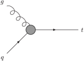
Figure 1: Strong anomalous production of single top at hadron colliders.

+

+

+

+

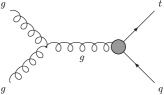
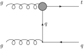
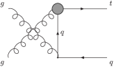
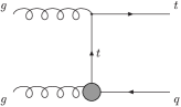
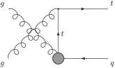
Figure 2: Strong anomalous production of single top plus a jet at hadron colliders.

The strong FCNC in Eq. (1) can produce a single top (Fig. (1))  [15] or a single top plus a jet (Fig. (2))  [16]. These are the two lowest order strong anomalous processes and must then allow for the best determination of the new strong vertices. In the second case collisions with initial quarks (or with a gluon and a quark) must be also summed up. At LHC, however, the probability of colliding two gluons is almost an order of magnitude higher than that of two quarks. These vertices can also produce events with a single top plus a $Z$ boson or a photon (Fig. (3))  [17]. In Table 1 we gather the bounds on the strong anomalous couplings derived from these processes if no signal is observed. These limits give also an indication of the precision which can be reached in each case.

		$\zeta_{tu}$	$\zeta_{tc}$
$pp\rightarrow t\rightarrow l\nu b$		$7\times 10^{-4}$	$2\times 10^{-3}$
$pp\rightarrow tj\rightarrow l\nu bj$		$1.5\times 10^{-3}$	$3\times 10^{-3}$
$pp\rightarrow Zt\rightarrow l^{+}l^{-}l\nu b$		$7\times 10^{-3}$	$1.5\times 10^{-2}$
$pp\rightarrow\gamma t\rightarrow\gamma l\nu b$		$3\times 10^{-3}$	$7\times 10^{-3}$

Table 1: Reachable bounds on the strong anomalous couplings (Eqs. (1,2)) at LHC with an integrated luminosity of $10\ {\rm fb}^{-1}$. The first two lines are divided by $\sqrt{2}$ to correct for the use of a different statistics.

+

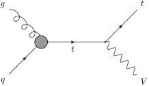
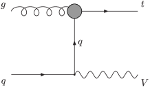
Figure 3: Strong anomalous production of single top plus a $Z$ boson or a photon at hadron colliders.

+

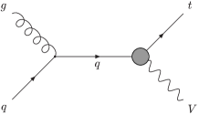
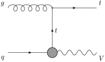
Figure 4: Electroweak anomalous production of single top plus a $Z$ boson or a photon at hadron colliders.

The lowest order process involving the weak and electromagnetic FCNC in Eq. (1) is $Vt$ production, $V=Z,\gamma$, but in this case with a standard (anomalous) strong (electroweak) vertex (Fig. (4))  [17]. The top and the $Z$ boson both decay before detection. Then we must specify their decay modes to define the sample we are interested in. The most significant $Zt\ (\gamma t)$ channel is $l^{+}l^{-}l\nu b\ (\gamma l\nu b),\ l=e,\mu,\$ because although it has a small branching ratio $1.5\%\ (21.8\%)$, it has also a small background $ZWj\ (\gamma Wj)$. In Table 2 we collect the corresponding bounds if no signal is observed. At Tevatron $\nu\bar{\nu}jjb$ is more significant because in this case the expected number of events is smaller and this channel has a larger branching ratio $13.6\%$ and the backgrounds $Zjjj,Wt,t\bar{t}$ are not very large.

		$X_{tu}$	$X_{tc}$		$\kappa_{tu}$	$\kappa_{tc}$		$\lambda_{tu}$	$\lambda_{tc}$
$pp\rightarrow Zt\rightarrow l^{+}l^{-}l\nu b$		0.022	0.045		0.014	0.034
$pp\rightarrow\gamma t\rightarrow\gamma l\nu b$								0.005	0.013

Table 2: Most stringent bounds on the electroweak anomalous couplings (Eqs. (1,2)) at LHC with an integrated luminosity of $10\ {\rm fb}^{-1}$.

Let us see now in an example, $pp\rightarrow Zt\rightarrow l^{+}l^{-}l\nu b$, how these limits are derived  [17]. To estimate the corresponding number of events we calculate the exact $2\rightarrow 5\ (gq\rightarrow Zt\rightarrow l^{+}l^{-}l\nu b)$ squared amplitude and use it to generate the events with the correct distribution. Afterwards we smear the lepton and jet energies and apply the trigger and detector cuts to the resulting sample to mimic the experimental set up. $b$-tagging is also required. Then we reconstruct the $Z\rightarrow l^{+}l^{-}$ and $t\rightarrow l\nu b$ invariant masses $M^{rec}_{Z}$ and $m^{rec}_{t}$, respectively (see Fig. (5)), and apply the kinematical cuts on $m^{rec}_{t}$, $p_{T}^{Z}$ (the $Z$ tranverse momentum) and $H_{T}$ (the total transverse energy). In this case signal and background have the same $M^{rec}_{Z}$ distribution and we do not gain anything cutting on this variable. The number of selected events is given in Table 3. Finally we use the adequate statistics  [19] to derive the expected bounds if no signal is observed.

		no cuts		with cuts
$gu\rightarrow Zt\ (\gamma^{\mu})$		5.0		4.8
$gc\rightarrow Zt\ (\gamma^{\mu})$		1.1		1.1
$gu\rightarrow Zt\ (\sigma^{\mu\nu})$		11.1		10.9
$gc\rightarrow Zt\ (\sigma^{\mu\nu})$		2.0		1.9
$ZWq_{u}$		4.9		1.4
$ZWq_{d}$		5.5		1.4
$ZWg$		4.7		1.1

Table 3: Number of $l^{+}l^{-}l\nu b$ events before and after kinematical cuts ($150\ {\rm GeV}\leq m_{t}^{rec}\leq 200\ {\rm GeV}$ and $200\ {\rm GeV}\leq H_{T}$) for the $Zt\rightarrow l^{+}l^{-}l\nu b$ signals and backgrounds at LHC with an integrated luminosity of $10\ {\rm fb}^{-1}$. $\gamma^{\mu}$ and $\sigma^{\mu\nu}$ stand for the corresponding non-zero anomalous vertex (Eqs. (1,2)). In this simulation we take $X_{tq}=0.02$ and $\kappa_{tq}=0.02$ for easy comparison.

Figure 5: Reconstructed top mass $m_{t}^{rec}$, $Z$ transverse momentum $p_{T}^{Z}$ and total transverse energy $H_{T}$ distributions before kinematical cuts for the $gu\rightarrow l^{+}l^{-}l\nu b$ signals and background at LHC with an integrated luminosity of $10\ {\rm fb}^{-1}$. $\gamma^{\mu}$ and $\sigma^{\mu\nu}$ stand for the corresponding non-zero anomalous vertex (Eqs. (1,2)). In this simulation we take $X_{tu}=0.02$ and $\kappa_{tu}=0.02$ for easy comparison.

4.2 Decay processes

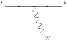
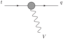
(a)		(b)

Figure 6: Standard (a) and anomalous (b) top decay.

Up to now we have assumed that the top decays as in the SM (diagram (a) in Fig. (6)), considering only the anomalous couplings in the production process. This is a good approximation because $t$ decays predominantly into $Wb$. However, the large number of $t\bar{t}$ pairs produced at future hadron machines (two gluon collisions (Fig. (7)) stand for $90\%$ of the total cross section and two quark collisions for the $10\%$) allows also to derive competitive bounds on top mixing if no anomalous $t$ decay is observed (diagram (b) in Fig. (6))  [13, 18].

+

+

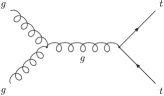
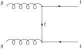
Figure 7: $gg\rightarrow t\bar{t}$ production.

5 Conclusions

We have reviewed present direct and indirect limits on top mixing, emphasizing that this can be large in simple SM extensions with vector-like quarks. Future hadron colliders will reduce these bounds to the per cent level if no anomalous signal is observed. $e^{+}e^{-}$ colliders will also set comparable limits searching for $e^{+}e^{-}\rightarrow t\bar{q}$ (Fig. (8)) and anomalous top decays  [20].

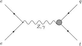
Figure 8: Electroweak anomalous production of single top plus a jet at $e^{+}e^{-}$ colliders.

References

• [1] S.L. Glashow, in Hadrons and their interactions, Proceedings Int. School of Physics ‘Ettore Majorana’, ed. A. Zichichi, Academic Press, New York, 1967; S. Weinberg, Phys. Rev. Lett. 19, 1264 (1967); A. Salam, in Elementary particle physics (Nobel Symp. No. 8), ed. N. Svartholm, Almqvist and Wilsell, Stockholm.
• [2] S.L. Glashow, J. Iliopoulos and L. Maiani, Phys. Rev. D2, 1285 (1970).
• [3] C. Burgess and H.J. Schnitzer, Nucl. Phys. B228, 464 (1983); C.N. Leung, S.T. Love and S. Rao, Z. Phys. C31, 433 (1986); W. Buchmüller and D. Wyler, Nucl. Phys. B268, 621 (1986); R.D. Peccei, S. Peris and X. Zhang, Nucl. Phys. B349, 305 (1991); R. Escribano and E. Massó, Nucl. Phys. B429, 19 (1994); see also S. Bar-Shalom and J. Wudka, hep-ph/9905407 and references there in.
• [4] F. Abe et  al., Phys. Rev. Lett. 80, 2525 (1998); see also T. Han, K. Whisnant, B.-L. Young and X. Zhang, Phys. Lett. B385, 311 (1996).
• [5] J.A. Aguilar-Saavedra, Ph D Thesis.
• [6] N. Cabibbo, Phys. Rev. Lett. 10, 531 (1963); M. Kobayashi and T. Maskawa, Prog. Theor. Phys. 49, 652 (1973).
• [7] C. Caso et  al., European Phys. Journal C3, 1 (1998).
• [8] Y. Nir and D. Silverman, Phys. Rev. D42, 1477 (1990); D. Silverman, Phys. Rev. D58, 095006 (1998).
• [9] F. del Aguila, J.A. Aguilar-Saavedra and R. Miquel, Phys. Rev. Lett. 82, 1628 (1999); F. del Aguila and J.A. Aguilar-Saavedra, hep-ph/9906461.
• [10] D. Karlen, in Proceedings of the International Conference on High Energy Physics ’98, Vancouver, 1998.
• [11] G.F. Tartarelli, CDF Collaboration, in Proceedings of International Europhysics Conference on High Energy Physics (HEP 97), World Scientific, 1997.
• [12] P. Abreu et al., Phys. Lett. B446, 62 (1999); DELPHI note 99-85; DELPHI note 99-146.
• [13] T. Han, R.D. Peccei and X. Zhang, Nucl. Phys. B454, 527 (1995).
• [14] F. del Aguila and M.J. Bowick, Nucl. Phys. B224, 107 (1983); G.C. Branco and L. Lavoura, Nucl. Phys. B278, 738 (1986);. P. Langacker and D. London, Phys. Rev. D38, 886 (1988); E. Nardi, E. Roulet and D. Tommasini, Nucl. Phys. B386, 239 (1992);. V. Barger, M.S. Berger and R.J.N. Phillips, Phys. Rev. D52, 1663 (1995); P.H. Frampton, P.Q. Hung and M. Sher, hep-ph/9903387, Phys. Rep. (in press) and references there in.
• [15] M. Hosch, K. Whisnant and B.-L. Young, Phys. Rev. D56, 5725 (1997).
• [16] T. Han, M. Hosch, K. Whisnant, B.-L. Young and X. Zhang, Phys. Rev. D58, 073008 (1998).
• [17] F. del Aguila, J.A. Aguilar-Saavedra and Ll. Ametller, Phys. Lett. B462, 310 (1999); F. del Aguila and J.A. Aguilar-Saavedra, hep-ph/9909222.
• [18] T. Han, K. Whisnant, B.-L. Young and X. Zhang, Phys. Rev. D55, 7241 (1997).
• [19] G.J. Feldman and R.D. Cousins, Phys. Rev. D57, 3873 (1998).
• [20] T. Han and J.L Hewett, Phys. Rev. D60, 074015 (1999); see also V.F. Obraztsov, S.R. Slabospitskii and O.P. Yushchenko, Phys. Lett. B426, 393 (1998).