Type II Seesaw and a Gauge Model for the Bimaximal Mixing Explanation of Neutrino Puzzles

Abstract

We present a gauge model for the bimaximal mixing pattern among the neutrinos that explains both the atmospheric and solar neutrino data via large angle vacuum oscillation among the three known neutrinos. The model does not include righthanded neutrinos but additional Higgs triplets which acquire naturally small vev’s due to the type II seesaw mechanism. A combination of global $L_{e}-L_{\mu}-L_{\tau}$ and $S_{3}$ symmetries constrain the mass matrix for both charged leptons and neutrinos in such a way that the bimaximal pattern emerges naturally at the tree level and needed splittings among neutrinos at the one loop level. This model predicts observable branching ratios for $\tau\rightarrow\mu\mu\mu$, which could be used to test it.
PACS: 14.60.Pq; 11:30.Hv; 12.15.Ff;

I Introduction

The observation of a deficit as well as of a zenith angle dependence in the flux of atmospheric muon neutrinos by the Super-Kamiokande [1, 2] collaboration has provided strong evidence that there are oscillations among the known neutrino species. The five solar neutrino experiments [3, 4] have added to this sense of excitement by their long standing result that there is also a deficit of the solar neutrinos, which can be given a simple explanation in terms of neutrino oscillations [5]. It thus appears certain that neutrinos have mass and they mix among each other. Although the details are fuzzy on the exact nature of the oscillations needed for the purpose, several very interesting scenarios exist. In particular, if the only laboratory indication of the neutrino oscillation by the Los Alamos collaboration (LSND) [6] is not included in the picture, there is a mixing scheme known as the bimaximal mixing, where both the solar and atmospheric data are explained by large mixing among the three known neutrinos [7]. In this picture, solar neutrino puzzle could either be solved via the large angle MSW mechanism [8] or via the vacuum oscillation mechanism [9] depending on the mass difference between the muon and the electron neutrinos. In this paper we will assume the vacuum oscillation between the $\nu_{e}$ and $\nu_{\mu}$ as the solution, which requires that their mass difference square must be $\sim 10^{-10}$ eV². The observed electron energy distribution as well as some hints of bi-annual variation of the solar neutrino flux by the Super-Kamiokande collaboration may be pointing in this direction.

If we accept this particular resolution of the neutrino puzzles, two major theoretical challenges emerge: one, how does one get naturally a theory that leads to the bimaximal mixing matrix and two, how does the same framework explain the tiny mass difference square ($\sim 10^{-10}$ eV²) needed for the purpose without fine tuning of parameters ? Our goal in this paper is to provide a simple model that generates both these features of the neutrino physics. Note that having a neutrino mass matrix of the right form to generate the bimaximal mixing pattern is by itself not sufficient since the desired mixing matrix is a combination of both the neutrino and the charged lepton mixing matrices i.e., $U^{\dagger}_{\ell}U_{\nu}$. Often it is assumed that $U_{\ell}={\bf 1}$ by appropriately choosing couplings in a theory to have certain values. This is of course not technically natural since radiative corrections could induce arbitrary values for those parameters thereby upsetting the neutrino mixing pattern. So what is really needed is (i) a neutrino Majorana mass matrix of the right form to generate the bimaximal mixing and (ii) a diagonal charged lepton mass matrix . It is the goal of this paper to present a model that satisfies both these criteria naturally. In this respect our model is different from others discussed in the literature (see later for detailed comparison).

One of the key ingredient in our work is the type II seesaw mechanism where the vev of a triplet Higgs becomes ultrasmall due to the presence of a high scale in the theory[10]. The presence of additional global symmetries in the model lead to a pattern of neutrino masses that leads to the bimaximal mixing among neutrinos while keeping flavor mixing among the charged leptons to be zero so that the bimaximal pattern dictated by the neutrino mass matrix that emerges is indeed natural.

Using the definition of the mixing matrix as

$$\left(\begin{array}[]{c}\nu_{e}\\ \nu_{\mu}\\ \nu_{\tau}\end{array}\right)=~{}U_{\nu}\left(\begin{array}[]{c}\nu_{1}\\ \nu_{2}\\ \nu_{3}\end{array}\right);$$ (7)

the bimaximal mixing corresponds to the mixing matrix $U_{\nu}$ given by[7]

$$U_{\nu}=\left(\begin{array}[]{ccc}\frac{1}{\sqrt{2}}&-\frac{1}{\sqrt{2}}&0\\ \frac{1}{2}&\frac{1}{2}&\frac{1}{\sqrt{2}}\\ \frac{1}{2}&\frac{1}{2}&-\frac{1}{\sqrt{2}}\end{array}\right).$$ (11)

As far as the neutrino masses go, they may be fully or partially degenerate or hierarchical as long as the mass differences fit the desired values. As mentioned, a convincing theoretical explanation of this elegant mixing pattern seems so far to have been elusive, although there exist many interesting attempts[11, 12, 13, 14, 15]. The problem becomes even more challenging when we demand that the solar neutrino puzzle be solved by the vacuum oscillation mechanism.

In this letter, we use the type II seesaw mechanism in conjunction with the global symmetry $S_{3}\times U(1)_{e-\mu-\tau}$ to show that both these properties can be realized in a natural manner. This leads us to a neutrino mass pattern where $m_{\nu_{\tau}}\ll m_{\nu_{\mu}}\simeq m_{\nu_{e}}\simeq\sqrt{\Delta m^{2}_{ATMOS}}\simeq 0.05$ eV and a generalized bimaximal pattern given by:

$$U_{\nu}=\left(\begin{array}[]{crc}\frac{1}{\sqrt{2}}&-\frac{1}{\sqrt{2}}&0\\ \frac{\cos\theta}{\sqrt{2}}&\frac{\cos\theta}{\sqrt{2}}&-\sin\theta\\ \frac{\sin\theta}{\sqrt{2}}&\frac{\sin\theta}{\sqrt{2}}&\cos\theta\end{array}\right).$$ (15)

II The Model

We consider an extension of the standard model where the fermion content is left unaltered but with a Higgs sector extended as follows: three doublets $\phi_{0},\phi_{1},\phi_{2}$, two triplets with $Y=2$ denoted by $\Delta_{1,2}$ and a charged isosinglet with $Y=+2$. The model has an $S_{3}$ symmetry (i.e. permutation group on three elements), under which the particles are assigned as shown in Table I.

Fields	$S_{3}$ transformation
($L_{\mu},L_{\tau}$)	2
($\mu_{R},\tau_{R}$)	2
$L_{e},e_{R}$	1
($\phi_{1},\phi_{2}$)	2
$\phi_{0}$	1
($\Delta_{1},\Delta_{2}$)	2
$\eta^{+}$	1’

• Table I: Transformation properties of the fields in the model under the $S_{3}$ group.

  We also impose an $L_{e}-L_{\mu}-L_{\tau}$ symmetry on the model. The Yukawa part of the Lagrangian in the leptonic sector consistent with these symmetries can be written as:

  $${\cal L}_{Y} = h_{1}\left(\bar{L}_{\mu}\mu_{R}+\bar{L}_{\tau}\tau_{R}\right)\phi_{0}+h_{2}\left[(\bar{L}_{\mu}\mu_{R}-\bar{L}_{\tau}\tau_{R})\phi_{1}+(\bar{L}_{\mu}\tau_{R}+\bar{L}_{\tau}\mu_{R})\phi_{2}\right]$$ (17)

  $$+h_{e}\bar{L}_{e}e_{R}\phi_{0}+fL_{e}\left(L_{\mu}\Delta_{1}+L_{\tau}\Delta_{2}\right)+f^{\prime}L_{\mu}L_{\tau}\eta+h.c.$$

  We will show later by a detailed examination of the Higgs potential for the system that there is a domain of parameters for which we get the following vevs of the fields:

  $$\langle\Delta^{0}_{1,2}\rangle~{}=~{}v^{T}_{1,2};\quad\langle\phi_{0}\rangle=v_{0};\quad\langle\phi^{0}_{1}\rangle=v_{1};\quad\langle\phi^{0}_{2}\rangle=0.$$ (18)

  Clearly, the pattern of $\phi$ vevs leads to a diagonal mass matrix for the charged leptons whereas the $\Delta$ vev’s leads to a Majorana mass for the neutrinos of the form:

  $$M_{\nu}=\left(\begin{array}[]{ccc}0&m_{1}&m_{2}\\ m_{1}&0&0\\ m_{2}&0&0\end{array}\right).$$ (22)

  As a consequence, diagonalization of the neutrino mass matrix is solely responsible for the neutrino mixings and one obtains the pattern given in the generalized bimaximal form [14, 15] (see Eq. (15)), with $\tan\theta=m_{2}/m_{1}=v_{2}^{T}/v_{1}^{T}$.

  Let us now address the question of neutrino masses. Clearly, to understand the small neutrino masses, one must have a tiny value for the vev of the $\Delta$ fields. This is achieved by the type II seesaw mechanism [10]. This is a generic mechanism, which can be illustrated by the following simple model that has only one $\phi$ and one $\Delta$. Consider the following Higgs potential for this system [10]:

  $$V(\phi,\Delta) = M^{2}\Delta^{\dagger}\Delta-\mu^{2}\phi^{\dagger}\phi+\lambda_{\phi}(\phi^{\dagger}\phi)^{2}+\lambda_{\Delta}\Delta^{\dagger}\Delta$$ (24)

  $$+\lambda_{\phi\Delta}\Delta^{\dagger}\Delta\phi^{\dagger}\phi+M_{\Delta\phi\phi}\Delta^{\dagger}\phi\phi~{}+~{}h.c.$$

  Let us choose $\mu\sim 100$ GeV and $M\sim M_{\Delta\phi\phi}\gg\mu$; in this case, the vev of $\langle\phi^{0}\rangle\approx\mu$ whereas the vev of $\langle\Delta^{0}\rangle\sim\frac{\mu^{2}}{M}\ll\mu$. This mechanism has been labeled type II seesaw and we see that if $M\simeq 10^{14}$ GeV, then we get $\langle\Delta^{0}\rangle\simeq 0.14$ eV. In the presence of more $\Delta$ fields and extra symmetries that our model has this mechanism still operates and we have a small mass (in the $0.1$ eV range) for the $\nu_{e}$ and $\nu_{\mu}$. The third eigenstate has zero mass. The $\nu_{\mu}$ and $\nu_{\tau}$ get mixed in the tree level and the mixing angle is near maximal unless we do fine tuning. As far as the $\nu_{\mu}$ and $\nu_{e}$ are concerned, they are degenerate and have opposite CP; therefore at the tree level their mass difference vanishes. We will show below that their mass difference arises at the one loop level but due to the presence of the high mass scale that gave rise to the type II seesaw mechanism, the mass difference $\Delta m^{2}_{e-\mu}$ is naturally suppressed to the level of $10^{-10}$ eV² without any unnatural fine tuning. The tree level mass matrix already explains the atmospheric neutrino puzzle due to the type II seesaw.

  Let us now turn to the explanation of the one loop contribution to the neutrino mass matrix. This is where the role of the $\eta$ boson becomes important. Let us first note that the masses of the doublet bosons are of order of the electroweak scale ($~{}100$ GeV) since their vevs must be of that order whereas that of the singlet $\eta$ and the triplet bosons are heavy (i.e., of order $10^{14}$ GeV). In order to generate the mass difference between the $\nu_{e}$ and $\nu_{\mu}$, we need nonzero entries for the $\mu\mu$ or $ee$ element. Both of them will violate the $L_{e}-L_{\mu}-L_{\tau}$ symmetry. This breaking is introduced by a soft term in the potential $\eta^{*}\phi_{1}\phi_{2}$ since $\eta$ has $L_{e}-L_{\mu}-L_{\tau}=-2$ and $\phi$’s are neutral under this global symmetry. This is a dimensional coupling and in accordance with our principle above that all fields which are not involved in the process of electroweak symmetry breaking are superheavy, we will choose this to be of order $M$. This leads to one loop graphs as in Figs. 1 and 2, which produce a neutrino mass matrix as follows:

  $$M_{\nu}=\left(\begin{array}[]{ccc}0&m_{1}&m_{2}\\ m_{1}&m_{\mu\mu}&m_{\mu\tau}\\ m_{2}&m_{\mu\tau}&m_{\tau\tau}\end{array}\right);$$ (28)

  where $m_{\mu\tau}\simeq m_{\mu\mu}\sin\theta\cos\theta$ and

  $$m_{\mu\mu}\simeq\frac{f^{\prime}h_{2}}{16\pi^{2}}\frac{m_{\tau}M_{\eta\phi\phi}v}{M^{2}}.$$ (29)

  For $M\simeq M_{\eta\phi\phi}$ and $f^{\prime}h_{2}\simeq 10^{-4}$, we get $m_{\mu\mu}\sim 10^{-9}$ eV, leading to $\Delta m^{2}_{e\mu}\simeq 10^{-10}$ eV², as is required to explain the solar neutrino puzzle via vacuum oscillation. Note that the tau neutrino picks up very tiny mass at one loop ($\sim 10^{-10}$ eV). This completes the derivation of the main result of our paper. The important point to note is that we need to choose the Yukawa couplings $f^{\prime}$ and $h_{2}$ individually only of order $10^{-2}$.

  Let us now compare our model with two existing ones[12, 13] in the literature. The model of Ma[12] has a similar field content to ours in all respects except that there is only one triplet field as against two in our paper. Thus inspite of the $S_{3}$ symmetry in that paper, the tree level mass matrix is very different and one does not have the bimaximal pattern at the tree level from the neutrino sector sector alone as in our case. On the other hand, the work of Ref.[13] uses only the $L_{e}-L_{\mu}-L_{\tau}$ symmetry, which allows arbitrary mixing angles in the charged lepton sector, which have to be set to zero at tree level. The addition of the $S_{3}$ symmetry as we do in this paper helps us to keep the charged leptons diagonal. There are also other major differences between the work of [13] and this work in the way the detailed dominant entries of the neutrino mass matrix arise- in our case at the tree level where as in [13] at the one loop model via the Zee-mechanism.

  III Rare Tau decays

  In this section we present a test of the model that involves flavor changing decays of the tau lepton. There are three sources of flavor changing effects in this model, i.e., via the exchanges of $\eta$, $\Delta$’s and $\phi_{2}$. At tree level, $\eta^{+}$ and $\Delta_{1,2}^{0,+}$ exchanges lead to $\mu$ or $\tau$ decay processes that include neutrinos as final products. However, as the masses of the exchange fields are very heavy ($\sim M$) such processes are highly suppressed. Therefore, only the diagrams that involve the exchange of the doublet fields are important.

  The general $\phi$ exchange tree level diagrams for Flavor Changing Neutral Currents (FCNC) are depicted in Figures 3 and 4. The internal lines in those figures represent the contributions of the general mixings in the scalar sector that come from the trilinear and quartic scalar couplings. In both of the figures, since one scalar field is necessarily a $\phi_{2}$ field, the $S_{3}$ symmetry restricts the involved vevs. In Fig. 3, for instance, it allows only $\langle\Delta_{2}\rangle$, regardless of whether the other field is $\phi_{0}$ or $\phi_{1}$. Thus, we estimate the amplitude of this diagram to be

  $$hh_{2}{\langle\Delta_{2}\rangle M_{\Delta\phi\phi}\over m_{\phi_{2}}^{2}m_{\phi_{0,1}}^{2}}\simeq h\cdot 10^{-6}~{}{\rm GeV}^{-2};$$ (30)

  where we have assumed as before that $M_{\Delta\phi\phi}\simeq M$, $m_{\phi}\simeq v$, $M_{\Delta\phi\phi}\langle\Delta\rangle\simeq v^{2}$ and taking $h_{2}=m_{\tau}/v\simeq 10^{-2}$. Here, $h$ represent the Yukawa coupling of the vertex on the right.

  For the diagram in Fig. 4, the vevs could be either $\langle\phi\rangle$ or $\langle\Delta\rangle$. Nevertheless, if we choose $\langle\phi\rangle$, again the $S_{3}$ symmetry play an important role by constraining one of them to be $\langle\phi_{2}\rangle$, which is zero, then the only contribution comes from the $\langle\Delta\rangle$ sector which is more suppressed already than the previous case by an extra $10^{-14}$ times the quartic coupling constant, which being dimensionless may be chosen of the order of one. There is no compensating factor such as large $M$ as in diagram in Fig. 3.

  Thus the only observable contribution to leptonic FCNC processes come from the diagram in Fig. 3. Matching the external leptonic legs in Fig. 3 with the terms in the Lagrangian, we see that only observable processes are of type $\tau\rightarrow\mu\mu\mu$ and $\tau\rightarrow\mu ee$, which have an amplitude of order $h10^{-6}~{}{\rm GeV}^{-2}$. Summing up the two contributions and assuming $\langle\phi_{0}\rangle\simeq\langle\phi_{1}\rangle$ and all dimensional couplings to be same, we get $h\simeq\frac{g_{2}m_{\mu}}{\sqrt{2}M_{W}}\simeq 10^{-3}$. This leads to the branching ratio for the decay mode $B(\tau\rightarrow\mu\mu\mu)\simeq 10^{-7}$. Since in our estimate we have assumed several couplings to be of order one, the prediction is uncertain within an order of magnitude but we do not expect it to be much smaller. This may be compared with the present experimental bounds [16] for the decays $\tau\rightarrow\mu\mu\mu$ which is $10^{-6}$. The branching ratio for the other allowed decay mode in our model $B(\tau\rightarrow\mu ee)\simeq 10^{-12}$ is small due to the fact that it involves the electron Yukawa coupling which is $\sim m_{e}/m_{W}$. Therefore, the three $\mu$ rare mode is the only observable FCNC processes in $\tau$ decays in this model and could therefore be used as a test.

  Let us stress that, an interesting feature of the present model is that the really rare process $\mu\rightarrow eee$ is automatically suppressed as it does not appear at the tree level. This is because, the only tree level coupling among electron and muon (or tau) involves $\Delta^{++}$, which does not mix with $\phi_{0}$, as would be required to get three electrons in the final states.

  At one loop order the most interesting process again appears in $\tau$ physics, i.e. the rare decay $\tau\rightarrow\mu\gamma$. The coresponding diagram is showed in Fig. 5. Now the decay width for this process is roughly estimated to be

  $$\Gamma\simeq{h_{2}^{2}h_{1}^{2}e^{2}\over 16\pi^{2}}{\langle\Delta_{2}\rangle^{2}M_{\Delta\phi\phi}^{2}m_{\tau}^{5}\over m_{\phi_{2}}^{4}m_{\phi_{0,1}}^{4}}\simeq 10^{-21}~{}{\rm GeV};$$ (31)

  giving a branching ratio of about $\sim 10^{-9}$, which is again below the current experimental bound [17] of $10^{-6}$.

  IV Analysis of the Higgs potential

  Lets us now show how $\langle\phi^{0}_{2}\rangle=0$ arises naturally from the potential. Given the irreducible representations (irreps) of $S_{3}$: $2_{x}=(x_{1},x_{2})$ and $2_{y}=(y_{1},y_{2})$, we may build the following singlets $1_{xy}=x_{1}y_{1}+x_{2}y_{2}$; $1^{\prime}_{xy}=x_{1}y_{2}-x_{2}y_{1}$; and the new doublet $2_{xy}=(x_{1}y_{1}-x_{2}y_{2},x_{1}y_{2}+x_{2}y_{1})$. Using this simple rules it is straightforward to find all possible $S_{3}$ and gauge invariant terms that include the scalar fields of the model. Such potential may be decomposed as $V=V(\phi)+V(\Delta)+V(\phi,\Delta)+V(\phi,\Delta,\eta)$. The last term involves all the expressions containing $\eta$. They do not contribute to the minimization of the potential, thus, it is not necessary to show them explicitly.

  As we already discussed above, the type II seesaw formula arises from $V(\Delta)+V(\phi,\Delta)$ by assuming large trilinear couplings. In this case $\langle\Delta\rangle$ becomes much much smaller than $\langle\phi\rangle$ and then we may neglect those terms in the analysis of the $\phi$ vevs. Defining $\Phi=(\phi_{1},\phi_{2})$, the relevant terms of the potential are then represented by

  $$V(\phi) = \mu^{2}~{}1_{\Phi^{2}}+\mu_{0}^{2}~{}1_{\phi_{0}^{2}}+\lambda_{1}~{}(1_{\Phi^{2}})^{2}+\lambda_{2}~{}(1_{\phi_{0}^{2}})^{2}+$$ (33)

  $$\lambda_{3}~{}1_{\Phi^{2}}~{}1_{\phi_{0}^{2}}+\lambda_{3}~{}1_{\Phi^{4}}+\lambda_{5}(1^{\prime}_{\Phi^{2}})^{2}+\lambda_{6}~{}1_{\Phi^{3}}~{}1_{\phi_{0}};$$

  where $1_{x^{n}}$ means the singlet built by using $n$ $x$ irreps. By examing $V(\phi)$ we may see that all the terms except the last one obey an accidental $U(1)_{\alpha}$ symmetry, which makes itself evident if we parametrize the vevs as

  $$\left(\begin{array}[]{c}\langle\phi_{1}\rangle\\ \langle\phi_{2}\rangle\end{array}\right)=v\left(\begin{array}[]{c}\cos\alpha\\ \sin\alpha\end{array}\right).$$ (34)

  Then, in terms of these parameters, the potential reduces to

  $$V(\phi)=V(v,\langle\phi_{0}\rangle)+\lambda_{6}\langle\phi_{0}\rangle v^{3}\cos\alpha.$$ (35)

  If the last term was absent, the minimum would exhibit a flat direction and an ensuing Goldstone boson. However, the last term breaks this extra symmetry explicitly and removes the flatness. Moreover, from this expression it is now straightforward to see that the potential gets its minimum for $\alpha=0$ ($\pi$) if $\lambda_{6}<0$ ($>0$), which means that $\langle\phi_{2}\rangle=0$, as we expected. It is worth pointing out that this special effect in the potential does not appear on the $\Delta$ sector, since it is just a consequence of the presence of the extra singlet $\phi_{0}$. As a matter of fact, $V(\Delta)$ is totally $U(1)_{\theta}$ symmetric while $V(\phi,\Delta)$ contains several terms that break explicitly such symmetry in a less trivial way, then avoiding a null value of $\langle\Delta_{2}\rangle$, and giving the pattern of neutrino masses.

  V Conclusions

  We have presented a model of neutrino masses based on the permutation symmetry $S_{3}$ in conjunction with the $L_{e}-L_{\mu}-L_{\tau}$ symmetry which leads to the bimaximal mixing pattern at the tree level and explain atmospheric oscillations through the hierarchy $m_{\nu_{\tau}}\ll m_{\nu_{\mu}}\simeq m_{\nu_{e}}$. The naturalness of the bimaximal mixing follows from the fact that the tree level mass matrix of the charged leptons is diagonal while the neutrino Majorana mass has a specific form dictated by the type II seesaw mechanism and the above symmetries. The soft breaking of the $L_{e}-L_{\mu}-L_{\tau}$ symmetry by the scalar potential through a coupling of the scalar doublets with an $S_{3}$ odd charged scalar, $\eta$, leads to the small entries in the neutrino mass matrix via radiative corrections. They are responsible for the small splitting in $\Delta m_{e\mu}^{2}$ needed to explain the solar neutrino deficit via vacuum oscillations. This model can be tested via the rare decay $\tau\rightarrow\mu\mu\mu$ whose branching ratio is predicted to be not too far below the current experimental limit[17].

  Acknowledgements. The work of RNM is supported by a grant from the National Science Foundation under grant number PHY-9802551. The work of APL is supported in part by CONACyT (México). The work of CP is supported by Fundação de Amparo à Pesquisa do Estado de São Paulo (FAPESP).

  

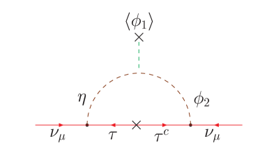
  FIG. 1.: One loop correction that generates the diagonal mass term $m_{\mu\mu}$. A similar diagram provides $m_{\tau\tau}$.

  
  

  

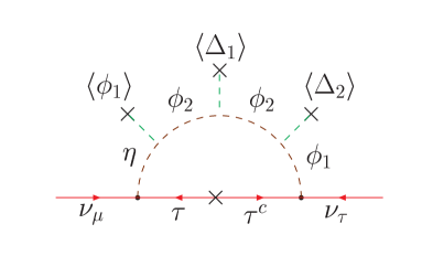
  FIG. 2.: One loop correction that generates the mass term $m_{\mu\tau}$.

  
  

  

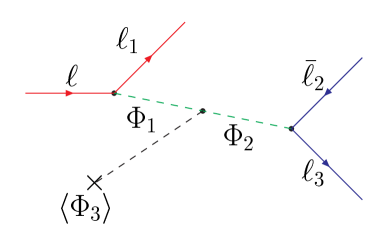
  FIG. 3.: Generical Feynman diagram responsible for FCC in the model at tree level. The external lines are leptonic fields. The internal lines could in principle be any one of the scalars involved in the trilinear couplings allowed by the $S_{3}$ symmetry.

  

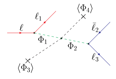
  FIG. 4.: Tree level FCC diagram involving the mixing produced by quartic scalar couplings.

  
  

  

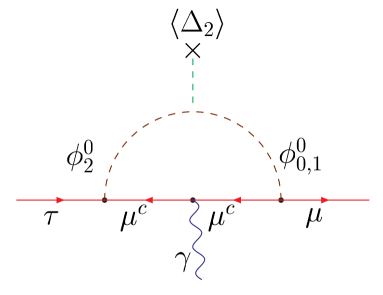
  FIG. 5.: One loop diagram that produce the $\tau\rightarrow\mu\gamma$ decay in the model.

REFERENCES

- [1] Y. Fukuda et al., Phys. Rev. Lett.81, (1998) 1562; idem. 81 (1998) 1158; Phys. Lett. B436 (1998) 33.
- [2] K.S. Hirata et al., Phys. Lett. B280 (1992) 146; R. Becker-Szendy et al., Phys. Rev. D 46 (1992) 3720; W. W. M. Allison et al., Phys. Lett. B 391 (1997) 491; Y. Fukuda et al, Phys. Lett. B 335 (1994) 237.
- [3] B. T. Cleveland et al. Nucl. Phys. B (Proc. Suppl.) 38 (1995) 47; K.S. Hirata et al., Phys. Rev. 44 (1991) 2241; GALLEX Collaboration, Phys. Lett. B388 (1996) 384; J. N. Abdurashitov et al., Phys. Rev. Lett. 77 (1996) 4708.
- [4] Super-Kamiokande collaboration, Phys. Rev. Lett. 81 (1998)1562.
- [5] For an extensive review and references, see the proceedings of the workshop on neutrinos, NOW98 hep-ph/9906251; for review of possible theories, see G. Altarelli and F. Feruglio, hep-ph/9905536; R. N. Mohapatra, hep-ph/9910365.
- [6] C. Athanassopoulos et al. Phys. Rev. Lett. 75 (1995) 2650; C. Athanassopoulos et al. Phys. Rev. C58 (1998) 2489.
- [7] F. Vissani, hep-ph/9708483; V. Barger, S. Pakvasa, T. Weiler and K. Whisnant, Phys. Lett. B437 (1998) 107; A. Baltz, A. S. Goldhaber and M. Goldhaber, Phys. Rev. Lett.81 (1998) 5730; M. Jezabek and Y. Sumino, Phys.Lett. B440 (1998) 327; G. Altarelli and F. Feruglio, Phys.Lett. B439 (1998) 112;
- [8] L. Wolfestein, Phys. Rev. D17 (1978) 2369; S.P. Mikheyev, A. Smirnov, Yad. Fiz. 42 (1985) 1441; Nuovo Cimento 9C (1986) 17.
- [9] For a recent summary and update on the solar neutrino puzzle, see J. Bahcall, P. Krastev and A. Y. Smirnov, Phys. Rev. D58 (1998) 096016; M. C. Gonzales-Garcia et al., hep-ph/9906469.
- [10] R. N. Mohapatra and G. Senjanović, Phys. Rev. D 23, 165 (1981); C. Wetterich, Nuc. Phys. B 187, 343 (1981); E. Ma and Sarkar, Phys. Rev. Lett. 80 , 5716 (1998).
- [11] R. N. Mohapatra and S. Nussinov, Phys. Rev. D 60, 013002 (1999); S. Davidson and S. F. King, Phys.Lett. B445 (1998) 191; C. S. Kim and J. D. Kim, hep-ph/9908435; C. H. Albright and S. Barr, Phys. Lett. B461 (1999) 218; H. Georgi and S. L. Glashow, hep-ph/9808293; H. B. Benaoum and S. Nasri, Phys. Rev. D60 (1999) 113003; M. Jezabek and Y. Sumino, Phys.Lett. B457 (1999) 139;
- [12] E. Ma, Phys. Rev. Lett.83 (1999) 2514; hep-ph/9909249.
- [13] A. Joshipura and S. Rindani, hep-ph/9811252; Phys.Lett. B464 (1999) 239.
- [14] R. Barbieri, L. Hall, A. Strumia and N. Weiner, JHEP 9812 (1998) 017.
- [15] See also: R. Barbieri, L. J. Hall, A. Strumia, Phys.Lett. B445 (1999) 407; Y. Grossman, Y. Nir and Y. Shadmi, JHEP 9810 (1998) 007; R. Barbieri, hep-ph/9901241; M. Jezabek, Y. Sumino, Phys. Lett. B457 (1999) 139; G. Altarelli, F. Feruglio, hep-ph/9905536; E. Kh. Akhmedov, hep-ph/9909217; E. Kh. Akhmedov, G. C. Branco and M. N. Rebelo, hep-ph/9911364.
- [16] Particle Data Group, C. Caso et al, The Eur. Phys. J. C3 (1998) 1.
- [17] CLEO collaboration, A. Anastassov et al., hep-ex/9908025.