Strong phases and $D^{0}-\overline{D}{}^{0}$ mixing parameters

Abstract

We argue that there could be significant $SU(3)$ violating resonance contributions to $D\to K\pi$ decays which would affect the extraction of the $D^{0}-\overline{D}{}^{0}$ mixing parameters from experiment. Such contributions can induce a strong phase in the interference between the doubly Cabibbo suppressed and the mixing induced Cabibbo favored contributions to the $D^{0}\to K^{+}\pi^{-}$ and $\overline{D}{}^{0}\to K^{-}\pi^{+}$ decays. Consequently, the interpretation of a large, CP conserving interference term can involve a large mass difference $\Delta M$ rather than a large width difference $\Delta\Gamma$.

(Revised December 1999)

I Introduction

Due to the smallness of the Standard Model (SM) $\Delta C=2$ amplitude, $D^{0}-\overline{D}{}^{0}$ mixing offers a unique opportunity to probe flavor-changing interactions which may be generated by new physics at short distances [1, 2, 3, 4, 5, 6, 7]. In fact, if $D^{0}-\overline{D}{}^{0}$ mixing is observed in the current round of experiments, it would unambiguously signal new flavor physics beyond the Standard Model. In particular, while the $D^{0}-\overline{D}{}^{0}$ mixing parameters $\Delta M$ and $\Delta\Gamma$ are small in the Standard Model, $\Delta M$ could be enhanced significantly by new short-distance interactions. An enhancement of $\Delta\Gamma$ is considerably less likely, since there are already strong constraints on the branching ratios of $D^{0}$ and $\overline{D}{}^{0}$ to common final states. Experimentally, $\Delta M$ and $\Delta\Gamma$ are measured by studying the time evolution of neutral $D$ mesons decaying to a particular final state. The two body decays $D\to K\pi$ are particularly popular, due to their relatively simple experimental signature [8].

The phenomenon of $D^{0}-\overline{D}{}^{0}$ mixing occurs because the neutral $D$ meson mass eigenstates do not coincide with the flavor eigenstates. The former are related to the latter by $|D_{1,2}\rangle=p|D^{0}\rangle\pm q|\overline{D}{}^{0}\rangle$, with $|p|^{2}+|q|^{2}=1$. Since it is the mass and not the flavor eigenstates which evolve diagonally, a state which is produced at $t=0$ as a $D^{0}$ meson may be detected at some later time $t$ as a $\overline{D}{}^{0}$. For the method of detecting $D^{0}-\overline{D}{}^{0}$ mixing involving the $D^{0}\to K\pi$ decay mentioned above, $D^{0}-\overline{D}{}^{0}$ mixing contributes through the sequence $D^{0}\to\overline{D}{}^{0}\to K^{+}\pi^{-}$, where the second stage is Cabibbo favored (CF). The search is complicated by the presence of a direct, doubly Cabibbo suppressed (DCS) process. Since the two sequences $D^{0}\to\overline{D}{}^{0}\to K^{+}\pi^{-}$ and $D^{0}\to K^{+}\pi^{-}$ lead to the same final state, one must study the time-dependent decay rate in order to separate these two contributions. These decay rates are given by

$$\Gamma(D^{0}(t)\to K^{+}\pi^{-}) = \textstyle{\frac{1}{4}}e^{-\Gamma t}\,|B|^{2}\,\left|{q}/{p}\right|^{2}\times$$ (2)

$$\ \left\{\left(\Delta M^{2}+\textstyle{\frac{1}{4}}\Delta\Gamma^{2}\right)t^{2}+\Big{(}2\mbox{Re}(\lambda)\Delta\Gamma+4\mbox{Im}(\lambda)\Delta M\Big{)}t+4|\lambda|^{2}\right\},$$

$$\Gamma(\overline{D}{}^{0}(t)\to K^{-}\pi^{+}) = \textstyle{\frac{1}{4}}e^{-\Gamma t}\,|\overline{B}|^{2}\,\left|{p}/{q}\right|^{2}\times$$ (4)

$$\ \left\{\left(\Delta M^{2}+\textstyle{\frac{1}{4}}\Delta\Gamma^{2}\right)t^{2}+\Big{(}2\mbox{Re}(\overline{\lambda})\Delta\Gamma+4\mbox{Im}(\overline{\lambda})\Delta M\Big{)}t+4|\overline{\lambda}|^{2}\right\},$$

where the quadratic terms ($t^{2}e^{-\Gamma t}$) arise from $D^{0}-\overline{D}{}^{0}$ mixing, the linear terms ($te^{-\Gamma t}$) describe interference between mixing and DCS contributions, and the constant terms ($e^{-\Gamma t}$) describe purely DCS decays. The importance of the linear term in Eq. (2) was emphasized in Ref. [9]. The mass and width differences are defined as $\Delta M=M_{2}-M_{1}$ and $\Delta\Gamma=\Gamma_{2}-\Gamma_{1}$. We also define

$$\lambda=|\lambda|e^{i(\delta+\theta)}=\frac{p}{q}\,\frac{A}{B}\,,\qquad\overline{\lambda}=|\overline{\lambda}|e^{i(\delta-\theta)}=\frac{q}{p}\,\frac{\overline{A}}{\overline{B}}\,,$$ (5)

to represent the convention-independent ratios of the amplitudes

$$A = \langle K^{+}\pi^{-}|H|D^{0}\rangle\,,\qquad\overline{A}=\langle K^{-}\pi^{+}|H|\overline{D}{}^{0}\rangle\,,$$ (6)

$$B = \langle K^{+}\pi^{-}|H|\overline{D}{}^{0}\rangle\,,\qquad\overline{B}=\langle K^{-}\pi^{+}|H|D^{0}\rangle\,.$$ (7)

The amplitudes $B$ and $\overline{B}$ are Cabibbo favored, while $A$ and $\overline{A}$ are doubly Cabibbo suppressed; $\delta$ and $\theta$ define strong and weak phases, respectively, of $\lambda$ and $\bar{\lambda}$. In the limit of unbroken $SU(3)$ symmetry, $A$ and $B$ are simply related by CKM factors, $A=(V_{cd}V_{us}^{*}/V_{cs}V_{ud}^{*})B$. In particular, $A$ and $B$ have the same strong phase [10], leading to $\delta=0$ in Eq. (5). Neglecting the small weak phases in the CKM elements of the first two generations, that is, setting $\theta\approx\arg(V_{cd}V_{ud}^{*}/V_{cs}V_{us}^{*})=0$, it is often assumed then that $\lambda$ and $\bar{\lambda}$ are real. The linear terms in Eq. (2) are therefore dominated by the terms proportional to $\Delta\Gamma$. More generally, for $\delta=0$ and any $\theta$, same-sign contributions to the interference terms in the two CP-conjugate processes of Eq. (2) are proportional to $\Delta\Gamma$. From this perspective, the experimental observation of such anomalously large coefficient of $t$ would be extremely surprising, since a substantial enhancement of $\Delta\Gamma$ is difficult to explain even in the presence of new physics. It is clearly important to explore the robustness of this conclusion.

This argument that $\delta$ vanishes, based on $SU(3)$ symmetry, has the virtue of being model-independent. However, $SU(3)$ is known experimentally to be broken badly in some $D$ decays, and therefore we might expect the relative strong phase of $A$ and $B$ not to vanish. The existing hadronic models which incorporate $SU(3)$ violation seem to prefer a small value of this phase, $\sin\delta\lesssim 0.2$, with most models giving $\sin\delta\lesssim 0.1$ [12, 13].

Do the small phases found in these models imply that the CP conserving part in the linear term is still dominated by $\Delta\Gamma$? Probably not. First, it is likely that $\Delta\Gamma$ is quite small, as it is generated by physical intermediate states and thus is not sensitive to any new $\Delta C=2$ interactions that might enhance $\Delta M$ [7]. In new physics scenarios of enhanced $D^{0}-\overline{D}{}^{0}$ mixing, $\Delta M\gg\Delta\Gamma$, and hence any nonzero coefficient of $\Delta M$, even if fairly small, permits it to dominate the linear term.

Second, these hadronic models may well not have enough $SU(3)$ violation in them, which is crucial since the phase $\delta$ is an $SU(3)$ violating effect. In particular, they may have difficulty accomodating the observed rates for the very mode used for the $D^{0}-\overline{D}{}^{0}$ mixing studies. The ratio [14]

$$R=\frac{{\cal B}(D^{0}\to K^{+}\pi^{-})}{{\cal B}(\overline{D}{}^{0}\to K^{+}\pi^{-})}\left|\frac{V_{ud}V_{cs}^{*}}{V_{us}V_{cd}^{*}}\right|^{2}$$ (8)

is unity in the $SU(3)$ symmetry limit. However, the world average for this ratio is [8, 14, 15, 16]

$$R_{\rm exp}=1.58\pm 0.49\,,$$ (9)

computed from the individual measurements using the standard methods of Ref. [22]. It is quite possible that $SU(3)$ is badly broken in $D\to K\pi$ transitions, in which case a significant strong phase of $\lambda$ would be a natural consequence.

It has been suggested that large $SU(3)$ violation in $D\to K\pi$ could be accomodated in a factorization approach by a conspiracy of individually small $SU(3)$ violating effects [12]. However, the use of the factorization anzatz is at least dubious in $D$ decays. It is also interesting to note that new experimental data on $D$ decay form factors [17],

$$\left|{f_{+}^{D\pi}}/{f_{+}^{DK}}\right|^{2}=0.9\pm 0.3\pm 0.3\,,$$ (10)

seem to suggest that $f_{+}^{D\pi}(0)<f_{+}^{DK}(0)$, while the analysis of Ref. [12] requires the opposite inequality. In any case, one may doubt our ability to predict accurately even the magnitude of the ratio of DCS to CF amplitudes. The phase $\delta$ is presumably still more uncertain.

The purpose of this paper is to make this suggestion concrete, by displaying a simple model in which $\lambda$ can easily have a significant strong phase. The model is based on the hypothesis of significant contributions to $D^{0}\to K^{+}\pi^{-}$ and $\overline{D}{}^{0}\to K^{+}\pi^{-}$ from nearby resonances. A deviation of $R_{\rm exp}$ from unity would imply, within our model, that the resonance couplings violate $SU(3)$ symmetry, in which case a large strong phase difference between the amplitudes $A$ and $B$ is a generic consequence. Therefore, it is unjustifiable to neglect the term proportional to ${\rm Im}\lambda\cdot\Delta M\cdot te^{-\Gamma t}$ in the time-dependent decay rate, even in the CP limit. No prejudice whatsoever about the phase of $\lambda$ should pollute the experimental analysis.

II Resonances as a source for strong phases

Our goal is to investigate the possible effects of broken flavor $SU(3)$ on the relative strong phases of the CF and DCS amplitudes $A$ and $B$. We will exploit the fact that the mass of the $D$ meson is small enough that it lies in the region populated by light quark resonances [7, 18, 19, 20]. (In this respect, $D$ decays are very different from $B$ decays, which lie far above the light resonance region. See Ref. [21] for a recent review.) It is therefore quite conceivable that a strong phase difference is generated by processes in which these resonances appear as $s$ channel intermediate states. If there is large $SU(3)$ violation related to these resonance effects, the phase difference $\delta$ could also be large.

For the sake of simplicity, we will assume that all or most $SU(3)$ violation in $(D^{0},\overline{D}{}^{0})\to K^{+}\pi^{-}$ comes from resonance contributions to the decay. Rather than modeling the resonance couplings directly, in our model we will fit them to the value of $R_{\rm exp}$. This is clearly an approach designed to maximize $SU(3)$ violation in the resonance contributions, which will typically maximize the phase difference $\delta$. Our point is not that we consider it likely that such a simple model accounts accurately for the phenomenology of these decays. Rather, it is, first, that these resonance contributions are generically present, and second, that without any tuning of the parameters it is quite possible to generate nonnegligible $\delta$. Therefore, we would argue, the existence of models in which $\delta$ is found to be small is hardly sufficient for one to conclude that this is not the case.

For the decays at hand the most important resonances are the “heavy kaons” of positive parity, $K^{*}(1430)$ and $K^{*}(1950)$. Both of these resonances are quite broad, $\Gamma(K^{*}(1430))=287\pm 10\pm 21$, and $\Gamma(K^{*}(1950))=201\pm 34\pm 79$ [22]. We will refer to $K^{*}(1430)$ and $K^{*}(1950)$ generically as “$K_{H}$.” We emphasize that the positions of these resonance poles are not very well established.

We will introduce an effective phenomenological coupling of the light quark resonance to a $D^{0}$ or $\overline{D}{}^{0}$ meson, which we will fit to the experimental data. We note in passing that most models of final state interactions in $D$ decays employ resonance dominance in some form (however, see also Ref. [23]). For instance, Refs. [24, 25] employ a set of two body intermediate states which rescatter to the final state via a resonance. Essentially, the coupling of the resonance to the $D$ meson is modeled by this two body contribution. In Refs. [7, 26] a similar coupling was taken to be dominated by a contact interaction. In our phenomenological approach, all of these contributions are absorbed into an effective $D-K_{H}$ coupling. For the non-resonance contribution to the decay, we will employ the Bauer-Stech-Wirbel (BSW) model [27]. In our picture all strong phases are generated by the nearby resonances. We will focus on the effect of the closest resonance, $K^{*}(1945)$.

We will not make any assumptions about the size of $SU(3)$ violation in the couplings of $K_{H}$ to $D^{0}$ and $\overline{D}{}^{0}$. We will find from our fit that the violation is large. While we propose no explicit mechanism to account for this, such a scenario need not be unnatural. For instance, one can imagine an extension of the models presented in Refs. [24, 25]. In these models, $K_{H}$ is coupled to the charmed mesons via an intermediate state composed of two ground state mesons, such as $K\pi$, which is treated in the factorization approximation, and $SU(3)$ violation is generically small. However, one should, in general, also consider additional intermediate states involving higher excitations of kaons and pions. For example, a contribution of the $K^{*}_{H}(1430)\pi$ intermediate state is quite different in $D^{0}$ and $\overline{D}{}^{0}$ decays even in the factorization approach, due to the large differences in the values of the relevant form factors and decay constants. Moreover, phase space effects will differ for different intermediate states. Certainly some combination of these factors could induce an $SU(3)$ violating effective coupling of the $D$ meson to the $K_{H}$. If it is mediated by physical intermediate states, this coupling generally will be complex; however, for simplicity we will neglect this additional source of strong phases.

We begin with a general discussion of the strong phase $\delta$ as a function of the decay amplitudes, which we decompose as

$$A=A_{T}+A_{R}\,e^{i\phi}\,,\qquad B=B_{T}+B_{R}\,e^{i\phi}\,.$$ (11)

Here $A_{T}$ and $B_{T}$ are the “tree” (nonresonant) contributions, and $A_{R}\,e^{i\phi}$ and $B_{R}\,e^{i\phi}$ are the amplitudes induced by $K_{H}$. The $B$-amplitudes are CF while the $A$ amplitudes are DCS. We assume here that strong phases arise only from the $K_{H}(1945)$ propagator in the resonance contribution. Consequently we may take $B_{T}$ and $A_{T}$ to be real (in the absence of new physics which might generate a “weak” phase), and the phase $\phi$,

$$\tan\phi=-{\Gamma_{K_{H}}m_{D}\over m_{D}^{2}-m_{K_{H}}^{2}}=1.23\,.$$ (12)

to be the same in $B_{R}$ and $A_{R}$. In particular, we assume here that the $D-K_{H}$ and $\overline{D}-K_{H}$ effective couplings are real.

It is straightforward to express the strong phase difference $\delta=\delta_{B}-\delta_{A}$ in terms of the relative contributions of the “tree” processes and the phase of the resonance amplitude:

$$\tan\delta=\pm\sin\phi\,{\sqrt{|B/B_{T}|^{2}-\sin^{2}\phi}-\sqrt{|A/A_{T}|^{2}-\sin^{2}\phi}\over\sin^{2}\phi+\sqrt{|B/B_{T}|^{2}-\sin^{2}\phi}\,\sqrt{|A/A_{T}|^{2}-\sin^{2}\phi}}\,.$$ (13)

We parametrize the relative contribution of the resonance amplitude to the CF decay by

$$Z_{\rm res}\equiv{B_{R}/B_{T}}\,.$$ (14)

In the $SU(3)$ limit, $A_{R}/A_{T}=B_{R}/B_{T}$. We parametrize SU(3) violation by

$$Z_{SU(3)}\equiv{A_{R}/A_{T}\over B_{R}/B_{T}}\,,$$ (15)

that is, $A_{R}/A_{T}=Z_{\rm res}Z_{SU(3)}$. Then we may write

$$\tan\delta={\sin\phi Z_{\rm res}(1-Z_{SU(3)})\over 1+Z_{\rm res}^{2}Z_{SU(3)}+\cos\phi Z_{\rm res}(1+Z_{SU(3)})}\,.$$ (16)

We clearly see that $\tan\delta$ is not required to be negligible, as is commonly assumed. There are, however, three scenarios that could, in principle, lead to a small strong phase $\delta$:

(i) $\sin\phi\ll 1$, that is, no nearby resonance.

(ii) $Z_{\rm res}\ll 1$, that is, negligible resonance contribution.

(iii) $|Z_{SU(3)}-1|\ll 1$, that is, negligible $SU(3)$ violation.

As is obvious from Eq. (12), scenario (i) is not realized in nature. Next we will fit our model to experiment and find that there is no evidence at present that either (ii) or (iii) is realized.

III Modeling the strong phase difference

The starting point for our model of the decay rate is the effective weak Hamiltonian for $c$ decays,

$${\cal H}_{eff} = \frac{G_{F}}{\sqrt{2}}V_{cs}V_{ud}^{*}\bigg{[}C_{1}(\mu)\,\bar{s}\Gamma_{\mu}d\,\bar{u}\Gamma^{\mu}c+C_{2}(\mu)\,\bar{u}\Gamma_{\mu}d\,\bar{s}\Gamma^{\mu}c\bigg{]}$$ (18)

$$\mbox{}+\frac{G_{F}}{\sqrt{2}}V_{cd}V_{us}^{*}\bigg{[}C_{1}(\mu)\,\bar{d}\Gamma_{\mu}s\,\bar{u}\Gamma^{\mu}c+C_{2}(\mu)\,\bar{u}\Gamma_{\mu}s\,\bar{d}\Gamma^{\mu}c\bigg{]},$$

where $\Gamma^{\mu}=\gamma^{\mu}(1+\gamma^{5})$, and $C_{1}(m_{D})\simeq-0.514$ and $C_{2}(m_{D})\simeq 1.270$ in the scheme-independent prescription [24]. Within the framework of the BSW model, the nonresonant contributions are given by

$$A_{T} = a_{1}\frac{G_{F}}{\sqrt{2}}V_{cd}V_{us}^{*}f_{K}f_{+}^{D\pi}(m_{K}^{2})m_{D}^{2}\left(1-{m_{\pi}^{2}}/{m_{D}^{2}}\right),$$ (19)

$$B_{T} = a_{1}\frac{G_{F}}{\sqrt{2}}V_{cs}V_{ud}^{*}f_{\pi}f_{+}^{DK}(m_{\pi}^{2})m_{D}^{2}\left(1-{m_{K}^{2}}/{m_{D}^{2}}\right).$$ (20)

Here $f_{\pi(K)}$ is the pseudoscalar meson decay constant, $f_{+}^{D\pi(K)}$ is the semileptonic form factor for $D\to\pi(K)$ transitions, and $a_{1,2}=C_{2,1}+C_{1,2}/N_{c}$. In the $SU(3)$ limit, $f_{\pi}=f_{K},~{}f_{+}^{D\pi}(m_{K}^{2})=f_{+}^{DK}(m_{\pi}^{2})$, and $m_{\pi}=m_{K}$. For simplicity, we have dropped the numerically insignificant contribution to Eq. (19) from the $f_{-}$ form factor.

The resonance-mediated amplitudes are given by

$$A_{R} = \frac{g_{H}}{m_{D}^{2}-m_{K_{H}}^{2}+i\Gamma_{K_{H}}m_{D}}\,\langle K_{H}|H_{eff}|D^{0}\rangle\,,$$ (21)

$$B_{R} = \frac{g_{H}}{m_{D}^{2}-m_{K_{H}}^{2}+i\Gamma_{K_{H}}m_{D}}\,\langle K_{H}|H_{eff}|\overline{D}{}^{0}\rangle\,,$$ (22)

where $K_{H}=K^{*}(1950)$. Here $g_{H}$ is the coupling of the resonance $K_{H}$ to the final state $K^{+}\pi^{-}$, which may be obtained from the measured branching ratio of $(52\pm 14)\%$ for $K_{H}\to K^{+}\pi^{-}$. We write the weak matrix elements entering Eq. (21) as

$$\langle K_{H}|H_{eff}|D^{0}\rangle = a_{2}\frac{G_{F}}{\sqrt{2}}V_{cd}V_{us}^{*}m_{D}^{2}m_{K_{H}}^{2}\cdot a\,,$$ (23)

$$\langle K_{H}|H_{eff}|\overline{D}{}^{0}\rangle = a_{2}\frac{G_{F}}{\sqrt{2}}V_{cs}V_{ud}^{*}m_{D}^{2}m_{K_{H}}^{2}\cdot\bar{a}\,.$$ (24)

Here $a$ and $\bar{a}$ parameterize the effective couplings of $D^{0}$ and $\overline{D}{}^{0}$ to the resonance $K_{H}$. In the $SU(3)$ limit, $\bar{a}=a$ and the relative phase between $A$ and $B$ vanishes. If $SU(3)$ is broken, then $\delta a=\bar{a}-a\neq 0$, generating a relative strong phase between $A$ and $B$. The values of $\bar{a}$ and $\delta a$ can be obtained by fitting to the measured branching ratios ${\cal B}(D^{0}\to K^{+}\pi^{-})$ and ${\cal B}(\overline{D}{}^{0}\to K^{+}\pi^{-})$ [22]. Note that we do not include the usual “weak scattering” amplitude of the BSW model. Instead, this term is absorbed into our new resonance amplitudes $A_{R}$ and $B_{R}$. This is the most natural thing to do, since we are essentially proposing a significant resonance enhancement of this ordinarily small contribution.

For the calculation of $B_{T}$, we use $f_{\pi}=132$ MeV, $f^{D\pi}_{+}(0)=0.69$, and a pole form to extroplate $f_{+}$ to the correct kinematic point [27]. For the calculation of $A_{T}$, we assume $SU(3)$ symmetry in the nonresonant amplitudes, so $A_{T}=B_{T}\tan^{2}\theta_{C}$. Then we find $B_{R}$ and $A_{R}$ by fitting to the observed decay rates. We find $|B/B_{T}|^{2}=0.76$ and, for the central value of $R_{\rm exp}=1.58$, we find $|A/A_{T}|^{2}=1.24$. The expression (13) for the phase difference yields

$$\tan\delta=\pm 0.33\quad\Rightarrow\quad\sin\delta=\pm 0.31\,.$$ (25)

In this case, the two solutions for the resonance fraction are $Z_{\rm res}=-0.23$ and $-1.03$. We see that the inclusion of the resonance amplitudes can have a dramatic impact, even though the couplings $a$ and $\bar{a}$ are of the moderate size $|a|\sim|\bar{a}|\sim{\rm few}\times 10^{-2}$. The effect is amplified by the small denominators in Eq. (21) associated with the presence of the nearby resonance. The substantial $SU(3)$ violation in the central value of $R_{\rm exp}$ is reflected in the fit, with the two solutions yielding $Z_{SU(3)}=-0.70$ and $1.38$.

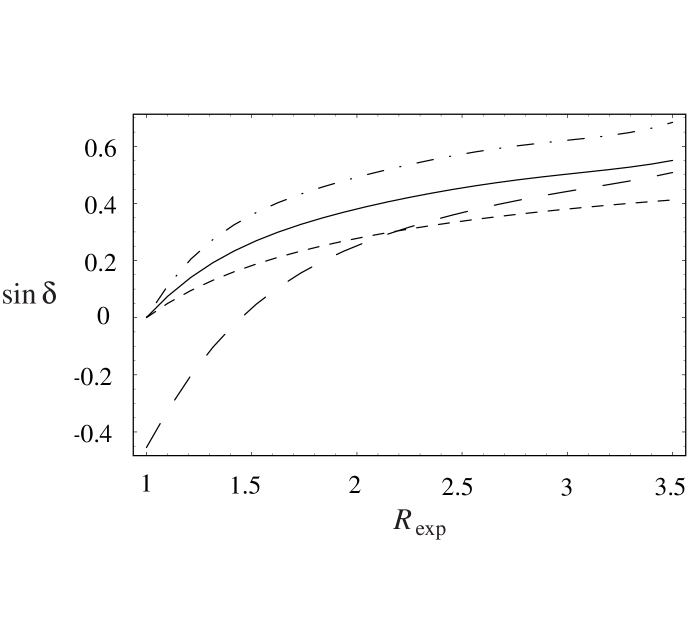
FIG. 1.: The variation of $\sin\delta$ with $R_{\rm exp}$. The solid line is our model with $\Gamma(K_{H})=200\,$MeV and $SU(3)$ symmetry in the “tree” amplitudes. The other lines demonstrate the robustness of the result if various assumptions are relaxed: (i) $SU(3)$ violation is incorporated into the BSW model (long dashed line); (ii) we set $\Gamma(K_{H})=260\,$ MeV (dashed-dotted line); (iii) the BSW model is modified so that $|B/B_{T}|^{2}=1.0$ (shorted dashed line). We show one of the two solutions for $\sin\delta$; the other has the same magnitude and the opposite sign.

The value of $\sin\delta$ can be rather large in this framework, and it depends strongly on the amount of $SU(3)$ violation observed in $R_{\rm exp}$. It also depends on the width of the resonance $K_{H}$, through the value of $\sin\phi$. The dependence on the details of the BSW model comes entirely through the value of $B_{T}$. Note that $a_{2}$ appears only in the combinations $a_{2}a$ and $a_{2}\bar{a}$, which are fit to experiment; hence our predictions are independent of $a_{2}$. Any variation in the model, such as including or dropping $1/N_{c}$ terms (which only has a moderate effect on $a_{1}$), can be absorbed into a change in $B_{T}$. Our model also can be modified to include the effects of $SU(3)$ violation in the BSW amplitudes $A_{T}$ and $B_{T}$. This is done by taking $f_{K}=162~{}\mbox{MeV}\neq f_{\pi}$ and $f_{+}^{DK}(0)=0.76\neq f_{+}^{D\pi}(0)$ [27].

In Fig. 1, we plot $\sin\delta$ as a function of $R_{\rm exp}$. We also show how the curves vary if we change the width of $K_{H}$ to $260\,$MeV, include $SU(3)$ violation in the BSW amplitudes, or set $|B/B_{T}|^{2}=1$ instead of 0.76. It is clear from the figure that values of $\sin\delta$ in the range 0.3 or larger are an entirely generic consequence of including the resonance $K_{H}$. We include in Fig. 1 large values of $R_{\rm exp}$, beyond the range in Eq. (9), to allow a comparison of our results to previous results in the literature that were derived for $R_{\rm exp}\sim 3$.

IV Discussion and Conclusions

Our model is sufficient to draw a qualitative conclusion about the phase of $\lambda$, if not a quantitative one. The issue at hand is really whether, in the CP limit, $\lambda$ can be taken to be approximately real in the analysis of $D^{0}-\overline{D}{}^{0}$ mixing. If this were so, then the observation of a substantial CP conserving linear term in $t$ in $\Gamma(D^{0}(t)\to K^{+}\pi^{-})$ would indicate the presence of a puzzling new physics contribution to $\Delta\Gamma$. Hence one must assess carefully the robustness of the assumption that $\delta\simeq 0$.

While there is a model-indepedent argument that in the $SU(3)$ (and CP) limit $\lambda$ is real, it is known that this symmetry is not always well respected in the $D$ system. In fact, a naive estimate of $SU(3)$ corrections would put them at the level of 30%, but $\sin\delta$ can only be ignored in the experimental analysis if it is considerably smaller than this. What really must be negligible is the combination $2\tan\delta\,\Delta M/\Delta\Gamma$. In the Standard Model, where $\Delta M/\Delta\Gamma\sim 1$, one ought to require at least $\sin\delta<0.1$. In new physics scenarios in which $\Delta M\gg\Delta\Gamma$, the requirement would be substantially stricter. In any case, to use $SU(3)$ as an argument for neglecting the phase would require actually that $SU(3)$ be respected unusually well. The current data on $R_{\rm exp}$ provide no support for such a scenario.

Another argument for a vanishingly small strong phase could be the absence of a mechanism for generating one. But given the existence of nearby resonances, this is not the case for the decay in question. It could also be that the resonance contributions are very small compared to the nonresonant ones, or that they respect $SU(3)$. Our fit shows that this is not necessarily the situation in the $D\to K\pi$ decays. We find therefore that there is no small parameter which would suppress the strong phases in these decays.

We have presented a model for the transition $D^{0}\to K^{\pm}\pi^{\mp}$ in which there is a significant $SU(3)$ violating contribution from an intermediate excited kaon resonance, and in which the strong phase of $\lambda$ is large. While we have designed this model, to some extent, to yield a significant strong phase difference, we have neither tuned parameters nor invoked an unnaturally large coupling to the resonance. In light of the ease with which this model produces a reasonably large phase, we would conclude that there is no good reason to assume $\sin\delta=0$ in any experimental analysis.

Finally, we note that while most of our analysis has been implicitly carried out in the framework of the Standard Model, our results are valid even in the presence of new physics. First, it is unlikely that the strong phase of $\lambda$ is affected by new physics. There are certainly extensions of the Standard Model, such as SUSY with ${\cal R}$ parity non-conservation, models with multiple Higgs doublets, and models with “exotic” quarks, which have new tree level flavor changing interactions that could contribute to the DCS decays. But the stringent existing constraints from $K^{0}-\overline{K}{}^{0}$ and $D^{0}-\overline{D}{}^{0}$ mixing preclude models in which such interactions are large enough to compete with standard $W$ exchange [28]. Second, while the Standard Model predicts that $\phi$ of Eq. (5) vanishes to an excellent approximation, the question of CP violating contributions to the interference term can be settled experimentally and does not require any model input. With $\phi\neq 0$, we would have contributions of opposite signs to the interference terms in $D^{0}\to K^{+}\pi^{-}$ and in $\overline{D}{}^{0}\to K^{-}\pi^{+}$. In the CP limit, the respective interference terms are equal. The presence of CP conserving interference terms can therefore be established experimentally, and then our comments of how to interpret it in terms of $\Delta\Gamma$ and $\Delta M$ apply.

- [1] A. Datta and D. Kumbhakar, Z. Phys. C27, 515 (1985).
- [2] A.A. Petrov, Phys. Rev. D56, 1685 (1997), hep-ph/9703335.
- [3] J. Donoghue, E. Golowich, B. Holstein and J. Trampetic, Phys. Rev. D33, 179 (1986).
- [4] L. Wolfenstein, Phys. Lett. 164B, 170 (1985).
- [5] H. Georgi, Phys. Lett. B297, 353 (1992), hep-ph/9209291.
- [6] T. Ohl, G. Ricciardi and E.H. Simmons, Nucl. Phys. B403, 605 (1993), hep-ph/9301212.
- [7] E. Golowich and A.A. Petrov, Phys. Lett. B427, 172 (1998), hep-ph/9802291.
- [8] M. Artuso et al. [CLEO Collaboration], hep-ex/9908040.
- [9] G. Blaylock, A. Seiden and Y. Nir, Phys. Lett. B355, 555 (1995), hep-ph/9504306.
- [10] L. Wolfenstein, Phys. Rev. Lett. 75, 2460 (1995), hep-ph/9505285.
- [11] E.M. Aitala et al. [E791 Collaboration], Phys. Lett. B421, 405 (1998) hep-ex/9711003.
- [12] L. Chau and H. Cheng, Phys. Lett. B333, 514 (1994), hep-ph/9404207.
- [13] T.E. Browder and S. Pakvasa, Phys. Lett. B383, 475 (1996), hep-ph/9508362.
- [14] D. Cinabro et al. [CLEO Collaboration], Phys. Rev. Lett. 72, 1406 (1994).
- [15] E.M. Aitala et al. [E791 Collaboration], Phys. Rev. D57, 13 (1998), hep-ex/9608018.
- [16] R. Barate et al. [ALEPH Collaboration], Phys. Lett. B436, 211 (1998), hep-ex/9811021.
- [17] J. Bartelt et al. [CLEO Collaboration], Phys. Lett. B405, 373 (1997), hep-ex/9703013.
- [18] E. Golowich, Phys. Rev. D24, 676 (1981).
- [19] F.E. Close and H.J. Lipkin, Phys. Lett. B372, 306 (1996), hep-ph/9511314.
- [20] M. Gronau, hep-ph/9908237.
- [21] A.A. Petrov, talk at The Chicago Conference on Kaon Physics (1999), hep-ph/9909312.
- [22] C. Caso et al. [Particle Data Group], Eur. Phys. J. C3, 1 (1998).
- [23] J.M. Gerard, J. Pestieau and J. Weyers, Phys. Lett. B436, 363 (1998), hep-ph/9803328.
- [24] F. Buccella et al. Phys. Rev. D51, 3478 (1995), hep-ph/9411286.
- [25] E.h. El aaoud and A.N. Kamal, hep-ph/9910327.
- [26] A.A. Petrov, in Upton 1997, Hadron spectroscopy, pp. 852-855, hep-ph/9712279.
- [27] M. Bauer, B. Stech and M. Wirbel, Z. Phys. C34, 103 (1987).
- [28] S. Bergmann and Y. Nir, JHEP 09, 031 (1999), hep-ph/9909391.