KLN theorem, magnetic mass,
and thermal photon production

Abstract

We study the infrared singularities associated to ultra-soft transverse gluons in the calculation of photon production by a quark-gluon plasma. Despite the fact that the KLN theorem works in this context and provides cancellations of infrared singularities, it does not prevent the production rate of low invariant mass dileptons to be sensitive to the magnetic mass of gluons and therefore the rate to be non perturbative.

1. Laboratoire de Physique Théorique LAPTH,
   UMR 5108 du CNRS, associée à l’Université de Savoie,
   BP110, F-74941, Annecy le Vieux Cedex, France

2. Brookhaven National Laboratory,
   Physics Department, Nuclear Theory,
   Upton, NY-11973, USA

LAPTH–756/99, BNL-NT–99/5

1 Introduction

It is widely accepted that infrared singularities are generally stronger in thermal field theories with bosons, compared to their counterparts at zero temperature. This is due to the singular behavior of the Bose-Einstein statistical weight at zero energy, which affects massless bosonic fields. As a consequence of these stronger singularities, only partial results exist concerning their cancellation in the calculation of observable quantities in thermal massless theories (see [1] for instance). So far, there is no general translation in the language of thermal field theory of the arguments given for this cancellation at $T=0$ by Kinoshita [2], and Lee and Nauenberg [3].

The resummation of hard thermal loops (HTL in the following) [4] cures partly this problem by giving a thermal mass to otherwise massless fields, like gauge bosons. Nevertheless, the static magnetic (transverse) modes remain massless in this framework and may still generate infrared singularities, as exemplified by the calculation of the fermion damping rate [5]. In QCD, it is believed that a thermal mass for the static transverse modes is generated non perturbatively at the scale $g^{2}T$, but this mass may be too small to be an efficient regulator.

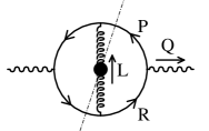
Figure 1: 2-loop dominant contribution to photon production. The blob indicates that the gluon propagator includes the resummation of hard thermal loops. The quark propagators include a thermal mass $M_{\infty}$, arising from the HTL resummation in the hard limit.

A particular area where this infrared problem becomes relevant is the thermal production of particles. In this paper, we focus mainly on the production of photons by a quark gluon plasma. The production rates are calculated as the imaginary part of a self-energy diagram evaluated at finite temperature [6], and are expected to be observable quantities that should come out finite in a consistent calculation.

In a recent study [7, 8, 9], it has been shown that 2-loop contributions involving the bremsstrahlung mechanism overwhelms 1-loop contributions for the production of a soft real photon. The insertion of an exchanged gluon in the hard quark loop (see Fig. 1) generates collinear singularities which are power like in 2-loop diagrams while they are only logarithmic in the 1-loop contributions: as a consequence, when these singularities are regularized by the resummation of the thermal mass $M_{\infty}\sim gT$ on the quark propagators, the two-loop diagrams get an enhancement by powers of $g^{-1}$, where $g$ is the strong coupling constant.

The contribution of the diagram of Fig. 1, although dominated by a soft gluon, is infrared finite. In fact, even the contribution of the transverse gluon is finite in this particular calculation, due to kinematical constraints. Indeed, it is trivial to see that the two delta functions corresponding to the cut quarks $\delta(P^{2}-M_{\infty}^{2})\delta((R+L)^{2}-M^{2}_{\infty})$ become $\delta(P^{2}-M_{\infty}^{2})\delta(R^{2}-M^{2}_{\infty})$ in the limit of vanishing $L$, and that the latter pair of delta functions do not have a common support if $M_{\infty}\not=0$: for the bremsstrahlung process we are considering here the energies $p_{0}$ and $r_{0}$ have the same sign and hence $P^{2}-M_{\infty}^{2}$ and $R^{2}-M^{2}_{\infty}$ cannot vanish simultaneously, whatever the value of $Q^{2}$. It is therefore kinematics, via the fermion thermal mass, that prevents infrared singularities in this particular topology by providing a natural cutoff of order $gT$ on the gluon momentum $L$. This statement was tested in [8] by studying the limit $M_{\infty}\to 0$. A stronger divergence was found in the transverse gluon contribution, indicating that $M_{\infty}$ played a role in the regularization of this potentially dangerous contribution.

But this kinematical cut-off does not apply to additional soft gluons one may insert in the quark loop, like in the diagram of Fig. 2 for instance.

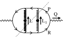
Figure 2: Example of three loop contribution for photon production. One of the gluons cannot become ultra-soft due to kinematics, and is displayed in boldface. The other, unconstrained, gluon is displayed as usual.

Indeed, in topologies involving more than one exchanged gluon, the kinematical argument given above constrains only the sum of the momenta of the cut gluons. Therefore, we know that $L+L_{1}$ cannot vanish, which tells us that (for instance) $L$ has a lower bound at the scale $gT$, but $L_{1}$ can still become arbitrary small and this leads to an infrared divergence for the cut depicted on Fig. 2 when the ultra-soft gluon is transverse. Indeed when compared to the 2-loop diagram, the additional gluon provides (i) two coupling constants, (ii) two quark propagators, (iii) a set of gluon spectral density and statistical weight and (iv) the phase-space of the additional gluon. Collecting everything, we can estimate by a crude power counting:

$${\rm(3-loop)}$$

$$\sim{\rm(2-loop)}\times g^{2}\int{d^{4}L_{1}}n_{{}_{B}}(L_{1})\rho(L_{1})$$

$$\qquad\qquad\times S(P+L_{1})S(R+L_{1})$$

$$\sim{\rm(2-loop)}\times g^{2}\int_{\mu}{l_{1}^{3}dl_{1}}{T\over{l_{1}}}{1\over{l_{1}^{2}}}{T\over{Tl_{1}}}{T\over{Tl_{1}}}$$

$$\sim{\rm(2-loop)}\times{{g^{2}T}\over\mu}\;,$$ (1)

where $\rho$ is the spectral function of the additional gluon, where $\mu$ is introduced as a regulator on the integral over $l_{1}$. We used the fact that the quarks are hard, and mostly on-shell because of the cut crossing the quark loop. It is important to stress here that each fermion propagator brings an extra factor $l_{1}$ in the denominator thus contributing to the infrared sensitivity of the above expression. The conclusions of this naive power counting are the following:

• If the additional gluon is longitudinal, its cutoff is a thermal mass of order $gT$ , and the corresponding contribution is suppressed by one power of $g$ compared to the 2-loop one.

• If the additional gluon is transverse it is natural to assume the regulator to be the magnetic mass $\mu\sim g^{2}T$, and we have ${\rm(3-loop)}\sim{\rm(2-loop)}$.

Therefore, it seems that if we keep adding transverse gluons in the quark loop, we generate contributions that are all of the same order of magnitude. This fact is very similar to the argument given by Linde for the breakdown of perturbation theory in thermal QCD, although in the different context of the calculation of the free energy [10].

There is nevertheless one reason why this power counting may be too naive. One should indeed keep in mind that this estimate is valid only for a given cut through the 3-loop diagram. It does not take into account potential compensations that may occur when one is summing all the possible cuts. In this paper, we are going to study in more detail this possibility, and its interplay with a magnetic mass at the scale $g^{2}T$.

2 Infrared cancellations

An important feature of the above example is the fact that the quark propagators participate in the overall infrared divergence of the diagram. In fact, if some quark propagators were not becoming singular in the IR limit, the diagram would have been finite by power counting. This can be generalized to a topology with an arbitrary number of exchanged gluons (but without 3- and 4-gluon vertices). Indeed, for these topologies, the number of loops $L$ is related to the number of gluons $n_{g}$ by:

$$L=1+n_{g}\;.$$ (2)

One of the $L$ loop integrals is an integration $d^{4}P$ over the quark momentum which is hard, and is not concerned by the IR problem. The remaining $L-1$ integrals are over the momenta of the $n_{g}$ soft gluons. The fact that $L-1=n_{g}$ tells that even if each gluon comes with the singular factor $n_{{}_{B}}(l^{o})\rho(L)$, it is accompanied by a phase space $d^{4}L$ which is enough to make the integral finite. For these topologies, it is the quark propagators which are ultimately responsible for the IR divergences. Indeed, it is trivial to see that if one quark propagator is cut, then some other quark propagators become infinite when the gluon momenta go to zero. This is the reason why we are going to focus on the quarks, and do not care about the gluon propagators.

It is rather easy to show that there are cancellations at the level of the quark propagators occuring in the calculation of the imaginary part of $\Pi^{\mu}_{\mu}$. Let us illustrate that in the reasonably general situation where we have a single quark loop to which are connected the two external photons, and an arbitrary number of internal gluons (but without non-abelian couplings, see Fig. 3). To simplify, we detail only the lower fermion line, and hide the details of the upper line in a complicated function we do not need to specify.

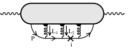
Figure 3: Generic configuration for which cancellations in the infrared sector occur. Again, the gluons all include the HTL correction. The gluons do not need to be parallel for the argument to work, since the gray area hides the details about how the gluons are attached to the upper quark line. The index $i$, running from $0$ to $n$, indicates which quark propagator is cut on the lower fermion line.

Since we are going to demonstrate cancellations among the various contributions to the dispersive part of the photon polarization tensor, it is convenient to work in the R/A formalism [11], in which cutting rules exist that are both very simple and very close to the $T=0$ ones [12]. Therefore, all the contributions to the imaginary part of $\Pi_{{}_{R}}$ can be obtained by cuts dividing the diagram into two connected pieces, each of these parts containing at least one external leg.

By summing over the index of the cut quark on the lower fermion line, the contribution of the diagram of Fig. 3 can be written as

$$\!\!\!\!\!\!\!\!\!\!\!\!A\equiv\int\!{d^{4}P}\Big{[}\!\prod_{i=1}^{n}{d^{4}L_{i}}n_{{}_{B}}(l^{0}_{i})\rho(L_{i})\;{\rm Trace}\Big{]}F(p^{0},p,\{L_{i}\})$$

$$\!\!\!\!\!\!\!\times\sum_{i=0}^{n}\delta((P+K_{i})^{2}-M^{2}_{\infty})\prod_{j\not=i}{1\over{(P+K_{j})^{2}-M^{2}_{\infty}}}$$ (3)

where the function $F$ hides all the details about the denominators on the upper quark line (as well as the fermionic statistical factors, which do not play any role in the following), and where we have defined

$$K_{i}\equiv\sum_{a=1}^{i}L_{a}\;.$$ (4)

We can now use the $\delta$ functions to perform explicitly the integral over $p^{0}$, which gives after splitting the propagators into positive and negative energy terms

$$\!\!\!\!\!\!\!\!A=\int{d^{3}{\tenimbf p}}\Big{[}\prod_{i=1}^{n}{d^{4}L_{i}}n_{{}_{B}}(l^{0}_{i})\rho(L_{i})\;{\rm Trace}\Big{]}\prod_{j=0}^{n}{1\over{2\omega_{j}}}$$

$$\!\!\!\!\!\!\times\sum_{\mathrel{\mathop{\kern 0.0pti=0}\limits_{\epsilon=\pm 1}}}^{n}\!F(\alpha_{i}^{\epsilon},p,\{L_{i}\})\prod_{j\not=i}\!\Big{[}{1\over{\alpha_{i}^{\epsilon}-\alpha_{j}^{+}}}-{1\over{\alpha_{i}^{\epsilon}-\alpha_{j}^{-}}}\Big{]}$$ (5)

where we denote $\omega_{i}\equiv\surd({({\tenimbf p}+{\tenimbf k}_{i})^{2}+M^{2}_{\infty}})$ and $\alpha_{j}^{\epsilon}\equiv-k_{j}^{0}+\epsilon\omega_{j}$. According to this definition, all the $\alpha_{i}^{\epsilon}$ become equal to $\epsilon\surd({\tenimbf p}^{2}+M^{2}_{\infty})$ when the gluon momenta go to zero. We see that denominators where both $\alpha_{i}$’s carry the same sign vanish in this limit. The IR singularities therefore show up in the vanishing denominators $\alpha_{i}^{\pm}-\alpha_{j}^{\pm}$. Only the second line in Eq. (5) is relevant in the following discussion, and it can be compactly rewritten as

$$\sum_{\mathrel{\mathop{\kern 0.0pti=0}\limits_{\{\epsilon_{i}=\pm_{1}\}}}}^{n}\!F(\alpha_{i}^{\epsilon_{i}},p,\{L_{i}\})\prod_{j\not=i}{{\epsilon_{j}}\over{\alpha_{i}^{\epsilon_{i}}-\alpha_{j}^{\epsilon_{j}}}}\;.$$ (6)

One can simply observe that for every denominator $\alpha_{i}^{\pm}-\alpha_{j}^{\pm}$ with numerator $F(\alpha_{i}^{\pm},p,\{L_{i}\})$ appears a denominator $\alpha_{j}^{\pm}-\alpha_{i}^{\pm}$ with a numerator $F(\alpha_{j}^{\pm},p,\{L_{i}\})$ (all the other denominators being the same). The simple poles therefore cancel trivially. This can be extended to the more complicated situation where more than two $\alpha_{i}$s tend to a common value, which amounts to prove that these denominators appear in a combination that remains finite for any configuration of the $\alpha_{i}$s. For that purpose, let us consider an expression like

$$F_{n}\equiv\sum_{i=0}^{n}F(\alpha_{i})\prod_{j\not=i}{1\over{\alpha_{i}-\alpha_{j}}}$$ (7)

and show that such a quantity is always finite provided some regularity property of the function $F$. The shortest way to see that is to notice that $F_{n}$ is the leading coefficient of the Lagrange polynomial of degree $n$ that interpolates between the points $(\alpha_{i},F(\alpha_{i}))$:

$$P_{n}(x)\equiv\sum_{i=0}^{n}F(\alpha_{i})\prod_{j\not=i}{{x-\alpha_{j}}\over{\alpha_{i}-\alpha_{j}}}=F_{n}\,x^{n}+\cdots$$ (8)

As such, $F_{n}$ is finite for every values of the $\alpha_{i}$’s if the function $F$ is $n$ times differentiable. Indeed, if several points $(\alpha_{i},F(\alpha_{i}))$ collapse into a single point of multiplicity $m$, the Lagrange polynomial has a finite limit, and coincides with $F$ and its first $m-1$ derivatives at this point. One can note that this argument also applies to insertions of self-energies on the quark line. Indeed, the only peculiarity of self-energy insertions is that they force several $\alpha_{i}$s to have the same value even if the $L_{i}$ do not tend to zero; and the above proof works for any configuration of the $\alpha_{i}$s, whatever the cause that makes them equal is.

Although the above argument has been presented in the case of a 2-point function, it still works for the dispersive part of any $n$-point function (just attach more photons or gluons to the shaded part of Fig. 3).

3 Competition with the magnetic mass

The result of the previous section is that the product of all the quark propagators remains finite in the IR sector when the sum over the cuts has been performed. When considering the imaginary part it shows that, for a fixed cut on the upper line, there is no singularity in the propagators of the lower line. The argument should be repeated for the upper line, which is made finite by summing over all the ways of cutting it. These cancellations between different cuts occur within a given topology, and correspond to compensation between real and virtual corrections. They can therefore be seen as a form of the KLN theorem.

We point out some differences with the usual version of the KLN theorem at zero temperature where the exchanged gluons are bare gluons. At finite temperature we deal with resummed gluons and the most dangerous divergences arise when cutting space-like transverse gluons which are shielded by a “small” magnetic mass. The time-like gluons are shielded with a “large” thermal mass of order $gT$ and do not lead to any infra-red problems in the context of this study.

We are now going to apply the above considerations to study explicitly the 3-loop example already presented in Fig. 2. As we have already seen in the introduction, one of the gluon momenta has a lower bound thanks to kinematics, while the other gluon is not constrained in the ultra-soft limit. Let us choose the gluon on the right (momentum $L_{1}$) to be ultra-soft while momentum $L$ remains soft. This kinematical constraint prevents the propagators of the lower quarks to become infinite when $L_{1}\to 0$: they always remain off-shell by some amount controlled by $M_{\infty}$. The constraint also simplifies the pattern of cancellation of infrared divergences in the upper line since the propagators of momentum $P+L+L_{1}\approx P+L$ when $L_{1}\to 0$ cannot diverge for the same reason. In consequence we need only the two cuts depicted on Fig. 4 to get rid of all the zeroes in the denominators.

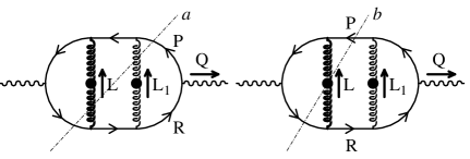
Figure 4: Notations used for the 3-loop contributions.

It turns out to be convenient to perform the change of variable $P+L_{1}\to P$ in the second contribution, as indicated on Fig. 4. Moreover, we neglect $L_{1}$ in front of $L$ whenever these two impulsions appear together (like in $L_{1}+L\approx L$). With these notations and approximations, one can readily see that the additional ultra-soft gluon brings the following factors, to be multiplied by the 2-loop integrand (i.e. the integrand for the diagram of Fig. 1), respectively for the cuts $(a)$ and $(b)$:

$$F_{a,b}=g^{2}\int{{d^{4}L_{1}}\over{(2\pi)^{4}}}(2P_{\sigma})(2R_{\rho})P^{\sigma\rho}_{{}_{T}}(L_{1})$$

$$\ \ \times{{\rho_{{}_{T}}(l_{1}^{0},l_{1})n_{{}_{B}}(l^{0}_{1})}\over{((P\pm L_{1})^{2}-M_{\infty}^{2})((R\pm L_{1})^{2}-M_{\infty}^{2})}}\;,$$ (9)

where $P^{\sigma\rho}_{{}_{T}}$ is the transverse projector, and $\rho_{{}_{T}}$ is the transverse spectral function of the gluon (only the transverse mode of the ultra-soft gluon is relevant, the other gluon can be transverse or longitudinal, as in the 2-loop calculation). The factors of form $P_{\sigma}/((P\pm L_{1})^{2}-M_{\infty}^{2})$ come from the fermion propagators in the hard momentum approximation. We can further simplify these factors by evaluating them at $P^{2}=M_{\infty}^{2}$ since they are to be multiplied by the 2-loop integrand which contains a $\delta(P^{2}-M^{2}_{\infty})$. Noticing that (see eq. (46) in [8])

$$P_{\sigma}R_{\rho}P^{\sigma\rho}_{{}_{T}}(L_{1})\approx-pr(1-\cos^{2}\theta_{1})\;,$$ (10)

where $\theta_{1}$ is the angle between the vectors ${\tenimbf p}$ and ${\tenimbf l}_{1}$, it is easy to perform the angular integral explicitly, which gives:

$$\!\!\!\!\int d\Omega_{1}{{1-\cos^{2}\theta_{1}}\over{((P\pm L_{1})^{2}-M_{\infty}^{2})((R\pm L_{1})^{2}-M_{\infty}^{2})}}$$

$$\quad\approx{\pi\over{prl_{1}^{2}}}\Big{(}\Big{[}x\!\pm{\Delta\over{4rl_{1}}}\Big{]}\ln\Big{|}{{2rl_{1}(x+1)\pm\Delta}\over{2rl_{1}(x-1)\pm\Delta}}\Big{|}-\!1\Big{)}$$

$$\quad\pm{{\pi(1-x^{2})}\over{pl_{1}\Delta}}\Big{[}\ln\Big{|}{{x+1}\over{x-1}}\Big{|}$$

$$\qquad\qquad\quad-\ln\Big{|}{{2rl_{1}(x+1)\pm\Delta}\over{2rl_{1}(x-1)\pm\Delta}}\Big{|}\Big{]}\;,$$ (11)

where we denote $x\equiv l_{1}^{0}/l_{1}$ and $\Delta\equiv 2P\cdot Q+Q^{2}$. The general result established in the previous section says that the sum over the cuts for this quantity should have a finite limit when $l_{1}\to 0$ at fixed $x$ (i.e. when the 4 components of $L_{1}$ tend to zero). One can see that this is not the case on the contributions of the individual cuts, since we have:

$$\!\!\!\!\!\!\!\!\int d\Omega_{1}{{1-\cos^{2}\theta_{1}}\over{((P\pm L_{1})^{2}-M_{\infty}^{2})((R\pm L_{1})^{2}-M_{\infty}^{2})}}$$

$$\mathrel{\mathop{\kern 0.0pt\approx}\limits_{l_{1}\to 0}}\pm{{\pi(1-x^{2})}\over{pl_{1}\Delta}}\ln\Big{|}{{x+1}\over{x-1}}\Big{|}\pm{{4\pi x}\over{pl_{1}\Delta}}\;,$$ (12)

(where we have neglected terms regular in $l_{1}$) but occurs trivially for the sum of the two cuts since the singular ($l_{1}^{-1}$) part drops out. The interesting quantity is in fact the scale at which this cancellation occurs. The only dimensional quantity to which $l_{1}$ can be compared with in the above expressions is $l_{1}^{*}\sim\Delta/r$. Carrying out the integration on $x,l_{1}$ we find the following finite result:

$$F_{a+b}\approx{{g^{2}Tr}\over{2\Delta}}\;.$$ (13)

When we add a magnetic mass $\mu$ into the game, we have two regularization mechanisms in competition, and we must compare the scales at which they operate, the most efficient being the one that has the largest scale. A convenient way to introduce the magnetic mass is via the following sum rule

$$\int\limits_{-\infty}^{+\infty}{{dx}\over{2\pi}}{{\rho_{{}_{T}}(l_{1},x)}\over{x}}B(x)\approx{{B(0)}\over{l^{2}_{1}+\mu^{2}}}\;,$$ (14)

which is a reasonable approximation if $B$ is not singular at $x=0$ and does not increase too much when $x$ becomes large. Adding the two cuts and approximating $n_{{}_{B}}(l^{0}_{1})\approx T/l_{1}x$, we find that the 2-loop integrand is to be multiplied by the factor

$$F_{a+b}\approx{{g^{2}Tr}\over{\pi^{2}\Delta}}\int\limits_{0}^{+\infty}{{l_{1}\,dl_{1}}\over{l_{1}^{2}+\mu^{2}}}\Big{\{}\ln\Big{|}{{\Delta+2rl_{1}}\over{\Delta-2rl_{1}}}\Big{|}$$

$$\qquad-{\Delta\over{rl_{1}}}\Big{[}{\Delta\over{4rl_{1}}}\ln\Big{|}{{\Delta+2rl_{1}}\over{\Delta-2rl_{1}}}\Big{|}-1\Big{]}\Big{\}}\;.$$ (15)

We can now give analytical limits for this factor in two cases. If the magnetic mass dominates over the scale $l_{1}^{*}$ defined above, we have

$$F_{a+b}\mathrel{\mathop{\kern 0.0pt\approx}\limits_{r\mu\gg\Delta}}{{g^{2}T}\over{\pi\mu}}\sim 1\;,$$ (16)

while in the opposite limit ($l_{1}^{*}\ll\mu$) we recover Eq. (13).

$$F_{a+b}\mathrel{\mathop{\kern 0.0pt\approx}\limits_{r\mu\ll\Delta}}{{g^{2}Tr}\over{2\Delta}}\ll 1\;.$$ (17)

Let us mention that if the additional gluon in Fig. 4 is longitudinal a similar calculation as above goes through where $\mu$ is to be replaced by the Debye mass of order $gT$, so that the factor $F_{a+b}$ is of order $g\ll 1$.

The conclusion is therefore the following:

• If the magnetic mass $\mu$ is the relevant regulator, then the 3-loop diagram gives a “correction” of order one to the prefactor of the 2-loop result, and this is likely to be the case for higher loop corrections also. In this regime, the photon production rate is sensitive to the magnetic mass, and one must resum an infinite series of diagrams.

• If on the contrary, the scale $\Delta/r$ dominates or if the regulator on the gluon propagator is the Debye mass, then the 3-loop diagrams lead to a negligeable correction to the 2-loop result, and it is expected that this hierarchy will be valid between 4-loop and 3-loop,… [8].

It remains now to make a bit more explicit the comparison between $\Delta/r$ and $\mu$. For that purpose, let us recall that the expression of $\Delta=2P\cdot Q+Q^{2}$ can be taken from the 2-loop calculation[7]:

$$\Delta\approx pq_{0}\Big{[}1-\cos\theta+{{M^{2}_{\rm eff}}\over{2p^{2}}}\Big{]}\;,$$ (18)

where $\theta$ is the angle between ${\tenimbf p}$ and ${\tenimbf q}$, and where

$$M_{\rm eff}^{2}=M^{2}_{\infty}+{{Q^{2}}\over{q_{0}^{2}}}pr\;.$$ (19)

Due to the extremely singular nature of the integral over $\theta$ [7, 8], the order of magnitude of $\Delta$ is $q_{0}M^{2}_{\rm eff}/p$. Taking into account the fact that $r\approx p+q_{0}$ and $p\sim T$, we divide the $(q,q_{0})$ plane in two regions where respectively $\mu$ or $\Delta/r$ dominates (see Fig. 5).

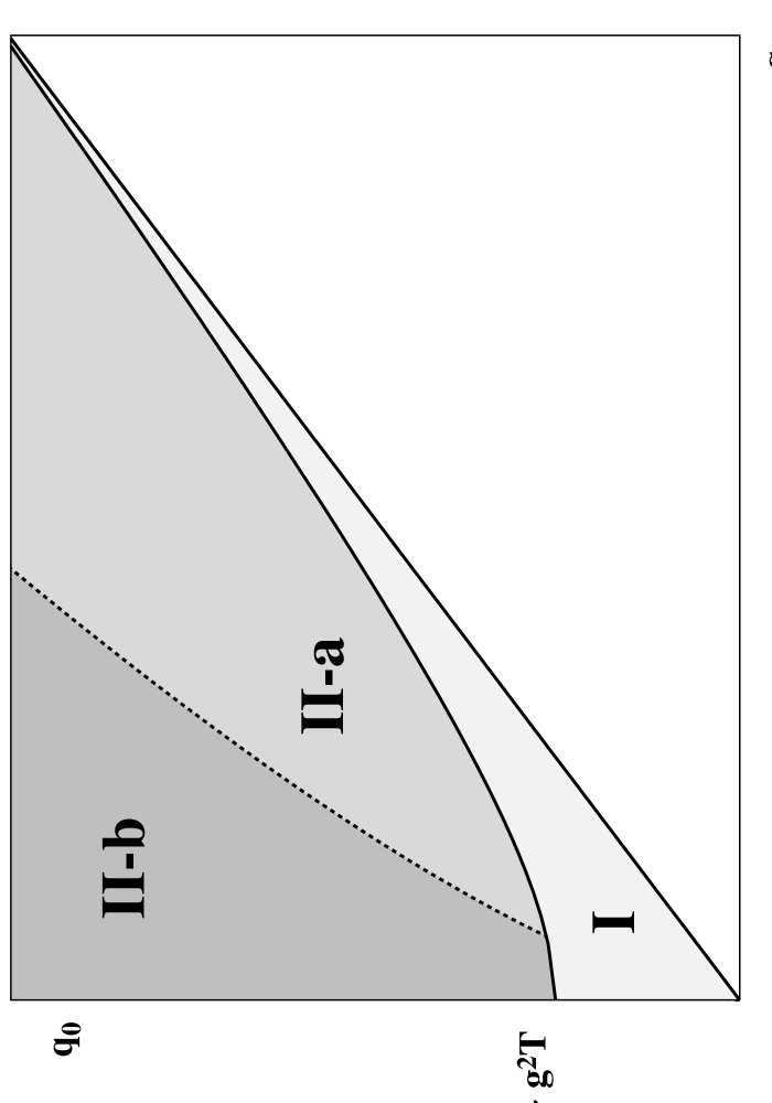
Figure 5: Comparison of $\mu$ and $\Delta/r$ in the $(q,q_{0})$ plane. In region I, the magnetic mass is the most important regulator, the 3-loop contribution is as large as the 2-loop one. In regions II-a and II-b, the magnetic mass is a subdominant regulator, and the higher-loop contributions are subdominant. In region II-b, $L$ can become hard and some of our approximations become invalid (see [9]).

In region I, i.e. roughly the region of small virtuality, the magnetic mass is the most important regulator and, as seen above, the 3-loop contribution is as large as the 2-loop contribution: the production mechanism becomes non-perturbative and resummations should be considered. Increasing the virtuality $Q^{2}$ of the photon increases $\Delta$ (see Eq. (19)) which eventually becomes the dominant cut-off and one enters region II where the infrared sensitivity of 3-loop (and higher loop diagrams) becomes subdominant.

In region II-b, the production mechanism receives a contribution from large gluon momentum and the approximations done in the previous calculations may become incorrect. However, it was found by an explicit calculation [9] that the expressions valid in region II-a could be safely extrapolated to the case of soft virtual photon at rest ($q=0$) in region II-b. However, there is the possibility that 3-loop diagrams give important contributions in region III due to hard gluon exchanges, but this is a different story.

4 Summary and outlook

In this paper, we have considered higher order corrections to photon production by a quark-gluon plasma, with emphasis on the infrared singularities due to ultra-soft transverse gluons. When one sums over all the possible cuts through a given abelian topology, there are cancellations that prevent the quark propagators from becoming infinite, making the higher-loop corrections infrared finite.

The generalization of this result to non-abelian topologies is not straightforward. Indeed, the above argument is flawed already at the stage of counting the number of gluon propagators. Loosely speaking, because of the 3- and 4-gluon couplings, the number of gluons can be larger than the number of independent momenta. The loop counting for QCD gives for the number of gluon integrations

$$L-1=n_{g}-(n_{3}+n_{4})\leq n_{g}\;,$$ (20)

where $n_{3}$ and $n_{4}$ are respectively the number of 3- and 4-gluon vertices. As a consequence, unlike in the abelian topologies for which $L-1=n_{g}$, the gluon propagators play an active role in the KLN compensations (if any), and much more elaborate arguments are required. As a side note, it is also impossible to apply in the thermal case the heuristic power counting argument of Poggio and Quinn [16], since some gluons have an infrared count of $-3$ (instead of $-2$ at $T=0$) because of the Bose-Einstein statistical weight.

We have also considered the possible competition of this mechanism of regularization with a hypothetical magnetic mass of order $g^{2}T$. The result is that there exists a region in the $(q,q_{0})$ plane (roughly speaking, for photons of small invariant mass) where the magnetic mass is the dominant regulator, and where the higher-loop corrections are as large as the two-loop result, and should be resummed.

Further extensions of this work include the treatment of non-abelian topologies, the study of resummations in the region where the magnetic mass dominates, the extension of the 2-loop calculation for hard massive photons, and also the study of how the finite lifetime of quarks in a plasma affects the collinear singularities found at 2-loop.

5 Acknowledgements

We thank R.D. Pisarski, F. Guerin and E. Braaten for useful discussions and comments. F.G. was supported by DOE under grant DE-AC02-98CH10886.

References

- [1] J. Cleymans, I. Dadic, University of Cape Town preprint UCT-TP-91/1987, Nov 1987; Z. Phys. C 42, 133 (1989). R. Baier, B. Pire, D. Schiff, Phys. Rev. D 38, 2819 (1988). T. Altherr, P. Aurenche, T. Becherrawy, Nucl. Phys. B 315, 436 (1989). T. Altherr, T. Becherrawy, Nucl. Phys. B 330, 174 (1990). T. Grandou, M. Le Bellac, J.L. Meunier, Z. Phys. C 43, 575 (1989). T. Grandou, M. Le Bellac, D. Poizat, Phys. Lett. B 249, 478 (1990); Nucl. Phys. B 358, 408 (1991). M. Le Bellac, P. Reynaud, Nucl. Phys. B 380, 423 (1992). A. Niegawa, Phys. Rev. Lett. 71, 3055 (1993). A. Niegawa, Mod. Phys. Lett. A 10, 379 (1995).
- [2] T. Kinoshita, J. Math. Phys. 3, 650 (1962).
- [3] T.D. Lee, M. Nauenberg, Phys. Rev. 133, 1549 (1964).
- [4] E. Braaten, R.D. Pisarski, Nucl. Phys. B 337, 569 (1990). E. Braaten, R.D. Pisarski, Nucl. Phys. B 339, 310 (1990). J. Frenkel, J.C. Taylor, Nucl. Phys. B 334, 199 (1990). E. Braaten, R.D. Pisarski, Phys. Rev. D 45, 1827 (1992). J. Frenkel, J.C. Taylor, Nucl. Phys. B 374, 156 (1992).
- [5] R.D. Pisarski, Phys.Rev. D 47 (5589) (1993). J.P. Blaizot, E. Iancu, Phys. Rev. Lett. 76, 3080 (1996). J.P. Blaizot, E. Iancu, Nucl. Phys. B 459, 559 (1996).
- [6] H.A. Weldon, Phys. Rev. D 28, 2007 (1983). C. Gale, J.I. Kapusta, Nucl. Phys. B 357, 65 (1991).
- [7] P. Aurenche, F. Gelis, R. Kobes, E. Petitgirard, Phys. Rev. D 54, 5274 (1996).
- [8] P. Aurenche, F. Gelis, R. Kobes, E. Petitgirard, Z. Phys. C 75, 315 (1997).
- [9] P. Aurenche, F. Gelis, R. Kobes, H. Zaraket, Phys. Rev D 58, 085003 (1998).
- [10] A.D. Linde, Phys. Lett. B 96, 289 (1980).
- [11] P. Aurenche, T. Becherrawy, Nucl. Phys. B 379, 259 (1992). M.A. van Eijck, Ch.G. van Weert, Phys. Lett. B 278, 305 (1992). M.A. van Eijck, R. Kobes, Ch.G. van Weert, Phys. Rev. D 50, 4097 (1994).
- [12] F. Gelis, Nucl. Phys. B 508, 483 (1997).
- [13] R.L. Kobes, G.W. Semenoff, Nucl. Phys. B 260, 714 (1985). R.L. Kobes, G.W. Semenoff, Nucl. Phys. B 272, 329 (1986).
- [14] P.F. Bedaque, A. Das, S. Naik, Mod. Phys. Lett. A 12, 2481 (1997).
- [15] To be presented elsewhere.
- [16] E.C. Poggio, H.R. Quinn, Phys. Rev. D 14, 578 (1976).