New Physics Effects from $e^{+}e^{-}\to f\bar{f}$ at a Linear Collider: the Role of $A_{LR,\mu}$

Abstract

We discuss New Physics effects in fermion pair production at LC in the framework of the “Z-peak subtracted approach”, a theoretical scheme that exploits the experimental measurements at LEP1 and SLC as input parameters. In particular, we discuss the role of the longitudinal polarization asymmetry $A_{LR,\mu}$ which turns out to be a very sensitive probe to New Physics of universal type. The extension of the method to non universal effects is discussed and an application is given in two examples: general contact interactions and low energy gravity models with graviton exchange.

I Introduction

The calculation of radiative corrections (RC) at future Linear Colliders (LC) facilities [1] is more difficult than at LEP1 energies: processes are no more dominated by Born diagrams and one loop corrections grow significantly with energy. The simple scenario describing $Z$ peak physics in terms of dominating single $Z$ resonant exchange is not valid at a LC with energy of the order of 1 TeV.

In such a situation, it seems difficult to give a simple parametrization of RC in the same spirit of LEP1 approaches like those leading for instance to Peskin-Takeuchi $S$, $T$ parameters [2] or Altarelli-Barbieri $\varepsilon_{1}$, $\varepsilon_{3}$ ones [3].

However, as we briefly review in this paper, there exists a simple scheme already exploited in LEP2 data analysis which, at least for New Physics of universal type (UNP), provides such a simple parametrization at LC energies too [4]. This is the so called “Z-peak subtracted approach” fully developed and illustrated in a series of dedicated papers [5] (see also [6] for a recent application to supersymmetric corrections). The basic idea of the scheme is to take LEP1 measurements as reference point and to describe virtual corrections at higher energies as deviations with respect to this point. With this aim, the conventional input parameter $G_{\mu}$ is replaced by certain observables measured at LEP or SLC on top of Z resonance. This approach is natural and effective: universal RC are parametrized in terms of three subtracted quantities where all $q^{2}$ independent effects disappear. The experimental error in the LEP1 measurements becomes thus a source of theoretical error of the scheme. Energy independent effects are constrained at low energy and left completely aside in the high energy analysis.

The plan of the paper is the following. In Sec. (II) we review some technical details on the Z peak subtracted approach. In Sec. (III) we list the expressions for UNP contributions in two important specific models and within our Z-peak subtracted parametrization. Sec. (IV) is devoted to the extension of the method to the case of two particularly simple models of non universal type, for which it is possible to perform an analogous analysis. In Sec. (V) we discuss the special role played by the longitudinal polarization asymmetry $A_{LR,\mu}$. Finally, in Sec. (VI) we summarize our results.

II Review of the $Z$-peak subtracted approach

Let us consider the process $e^{+}e^{-}\to l^{+}l^{-}$ for the production of a lepton pair. The analysis could be done for a generic fermion in the final state [5], but to simplify the discussion we consider here the simpler case of the leptonic channel. The invariant scattering amplitude receives radiative corrections from the one particle irreducible self energies, initial and final vertices and boxes as shown schematically in Fig. (1). The one loop amplitude can be written in the form of a modified Born expression

$$A(s,\theta) = \frac{i}{q^{2}}v_{\mu}^{(\gamma)}v^{(\gamma)\mu}(1-{\widetilde{F}}_{\gamma})+$$ (1)

$$+ \frac{i}{q^{2}-M_{0Z}^{2}}v_{\mu}^{(Z)}v^{(Z)\mu}\left(1-\frac{{\widetilde{A}}_{Z}}{q^{2}-M_{0Z}^{2}}\right)+$$ (2)

$$- \frac{2i}{q^{2}-M_{0Z}^{2}}v_{\mu}^{(\gamma)}v^{(Z)\mu}\frac{{\widetilde{A}_{\gamma Z}}}{q^{2}},$$ (3)

where we have introduced the photon and Z Lorentz structures

$$v_{\mu}^{(\gamma)}=-|e_{0}|\langle l_{2}|J_{\mu}^{(\gamma)}(0)|l_{1}\rangle,\ J_{\mu}^{(\gamma)}=\sum_{i}Q_{i}\bar{\psi}_{i}\gamma_{\mu}\psi_{i},$$ (4)

$$v_{\mu}^{(Z)}=-\frac{|e_{0}|}{2s_{0}c_{0}}\langle l_{2}|J_{\mu}^{(Z)}(0)|l_{1}\rangle,\ J_{\mu}^{(Z)}=\sum_{i}\bar{\psi}_{i}\gamma_{\mu}(g_{Vi}^{0}-\gamma_{5}g_{Ai}^{0})\psi_{i},$$ (5)

with $g_{Ai}^{0}=I_{3L,i}$, $g_{Vi}^{0}=I_{3L,i}-2Q_{i}s_{0}^{2}$. All the virtual contributions are hidden into the three quantities $\widetilde{F}_{\gamma}$, $\widetilde{A}_{Z}$ and $\widetilde{A}_{\gamma Z}$ after the projection of self energies, vertices and boxes on the proper $\gamma$ and $Z$ structures. This decomposition can be shown to be gauge invariant [7] as a consequence of the independence of these structures.

The explicit expression of the gauge invariant combinations is

$${\widetilde{F}}_{\gamma}=F_{\gamma}-2(\Gamma_{\mu}^{(\gamma)},v_{\mu}^{(\gamma)})-A^{Box}_{\gamma\gamma},$$ (6)

$$\frac{{\widetilde{A}}_{Z}}{q^{2}-M_{0Z}^{2}}=\frac{A_{Z}}{q^{2}-M_{0Z}^{2}}-2(\Gamma_{\mu}^{(Z)},v_{\mu}^{(Z)})-A^{Box}_{ZZ},$$ (7)

$$\frac{{\widetilde{A}}_{\gamma Z}}{q^{2}} = \frac{A_{\gamma Z}}{q^{2}}-(\Gamma_{\mu}^{(Z)},v_{\mu}^{(\gamma)})-\frac{q^{2}-M_{0Z}^{2}}{q^{2}}(\Gamma_{\mu}^{(\gamma)},v_{\mu}^{(Z)})+$$ (8)

$$- (q^{2}-M_{0Z}^{2})A^{Box}_{\gamma Z},$$ (9)

where the quantities $F_{i}(q^{2})$ ($i=\gamma,Z,\gamma Z$) have been extracted from the transverse part of the corresponding self energies $A_{i}(q^{2})$ according to

$$A_{i}(q^{2})=A_{i}(0)+q^{2}F_{i}(q^{2}),$$ (10)

and the notation $(\Gamma,\cdot)$ stands for the projection on the $\gamma$ and $Z$ structures.

The Z-peak subtracted prescription enters at this very point. Indeed, one can introduce the subtracted parameters (the subscript $el$ specifies the process $e^{+}e^{-}\to l^{+}l^{-}$ under consideration):

$${\widetilde{\Delta}\alpha}_{el}=\mbox{Re}(\tilde{F}_{\gamma}(0)-\tilde{F}_{\gamma}(q^{2})),$$ (11)

$$\tilde{I}_{Z,el}=\frac{q^{2}}{q^{2}-M_{Z}^{2}}\mbox{Re}(\tilde{F}_{Z}(q^{2},\theta)-\tilde{F}_{Z}(M_{Z}^{2},\theta)),$$ (12)

$$R_{el}=\tilde{I}_{Z,el}(q^{2})-\tilde{I}_{Z,el}(M_{Z}^{2}),$$ (13)

$$V_{el}=\mbox{Re}(\tilde{F}_{\gamma Z}(q^{2})-\tilde{F}_{\gamma Z}(M_{Z}^{2})),$$ (14)

and show that, at the one loop level, all the observables can be rewritten in terms of ${\widetilde{\Delta}\alpha}_{el}$, $R_{el}$ and $V_{el}$ by eliminating $G_{\mu}$ and introducing LEP measured quantities as new input parameters. To be specific, let us consider the simplest example, the cross section for $\mu^{+}\mu^{-}$ production. In this case (neglecting the $\gamma Z$ interference term) the following typical expression is obtained:

$$\sigma_{\mu} = \frac{4}{3}\pi q^{2}\left\{(\frac{\alpha}{q^{2}})^{2}(1+2{\widetilde{\Delta}\alpha}_{e\mu})+\frac{1}{(q^{2}-M^{2}_{Z})^{2}+M_{Z}^{2}\Gamma^{2}}\left(\frac{3\Gamma_{l}}{M_{Z}}\right)^{2}\times\right.$$ (15)

$$\times \left.\left(1-2R_{e\mu}-\frac{16(1-4\tilde{s}_{l}^{2})\tilde{s}_{l}\tilde{c}_{l}}{1+\tilde{v}_{l}}V_{e\mu}\right)\right\},$$ (16)

where the $Z$ widths $\Gamma$ and $\Gamma_{l}$ appear. The quantity $\tilde{v}_{l}$ is defined as $\tilde{v}_{l}(M_{Z}^{2})=1-4{\tilde{s}}_{l}^{2}(M_{Z}^{2})$ where $\tilde{s}^{2}_{l}=1-\tilde{c}_{l}^{2}$ is the effective mixing angle directly related to the measurement of asymmetries at the Z peak.

A similar discussion can be done in the case of hadronic observables, in particular the light quark-antiquark production cross sections and asymmetries. To extend the scheme, additional input parameters must be introduced like the Z widths and asymmetries into hadrons. In the end, the one loop effects turn out to be parametrized in terms of four (flavour dependent) functions [5]

$${\widetilde{\Delta}\alpha}_{ef},\qquad R_{ef},\qquad V_{ef}^{\gamma Z},\qquad V_{ef}^{Z\gamma}.$$ (17)

When New Physics effects are considered, these quantities are shifted:

$${\widetilde{\Delta}\alpha}_{ef}\to{\widetilde{\Delta}\alpha}_{ef}+{\widetilde{\Delta}\alpha}_{ef}^{NP},$$ (18)

and similarly for the other three. It is convenient to focus on those New Physics models that produce virtual contributions independent both on the final fermion flavour and on the scattering angle $\theta$. We denote by Universal New Physics (UNP) all such effects. Due to universality, the simplification $V^{\gamma Z}_{ef}=V^{Z\gamma}_{ef}$ occurs and the deviation with respect to the Standard Model can be parametrized by three functions of $q^{2}$ only (here, we are allowed to omit the $ef$ label)

$${\widetilde{\Delta}\alpha}^{UNP}(q^{2}),\qquad R^{UNP}(q^{2}),\qquad V^{UNP}(q^{2}).$$ (19)

By construction, these are subtracted quantities that must vanish at $q^{2}=0,M_{Z}^{2},M_{Z}^{2}$ respectively. We choose therefore to write our final parametrization will in terms of the three parameters

$$\delta_{z}(q^{2}),\qquad\delta_{s}(q^{2}),\qquad\delta_{\gamma}(q^{2}),$$ (20)

defined by

$$\widetilde{\Delta}\alpha^{UNP}(q^{2})=\frac{q^{2}}{M_{Z}^{2}}\ \delta_{\gamma}(q^{2}),\qquad R^{UNP}(q^{2})=\frac{q^{2}-M_{Z}^{2}}{M_{Z}^{2}}\ \delta_{z}(q^{2}),\qquad V^{UNP}(q^{2})=\frac{q^{2}-M_{Z}^{2}}{M_{Z}^{2}}\ \delta_{s}(q^{2}).$$ (21)

In the following sections we shall fix $\sqrt{q^{2}}=500\ \mbox{GeV}$ and consider specific NP models for which we derive bounds in the three dimensional space $(\delta_{z},\delta_{s},\delta_{\gamma})$.

III Models with Universal New Physics Corrections

In this Section, we discuss the specific form of the virtual one loop contribution to $\delta_{z}$, $\delta_{s}$ and $\delta_{\gamma}$ for two models where such corrections are of universal type: models with anomalous couplings and models of technicolor type, that is with strongly coupled resonances.

A Anomalous gauge couplings

As a first UNP model we consider one with anomalous gauge couplings (AGC) in the framework of [8] restricting our analysis to dimensions six effective terms in the Standard Model lagrangian with $SU(2)\times U(1)$ and $CP$ invariance. As is well known, there are 4 operators affecting the $WW\gamma$, $WWZ$ vertices at tree level and 5 operators that enter at the one loop level by renormalizing the coupling of the first four. In a general conventional and model independent analysis one must thus determine four parameters. However, as shown in [9], only two parameters ($f_{DW}$ and $f_{DB}$) survive in the Z-peak subtracted approach making the analysis and the fit to experimental data much more simple.

The explicit expression of the UNP contribution to $\delta_{z}$, $\delta_{s}$ and $\delta_{\gamma}$ are

$$\delta_{z}=8\pi\alpha\frac{M_{Z}^{2}}{\Lambda^{2}}\left(\frac{\tilde{c}_{l}^{2}}{\tilde{s}_{l}^{2}}f_{DW}+\frac{\tilde{s}_{l}^{2}}{\tilde{c}_{l}^{2}}f_{DB}\right),$$ (22)

$$\delta_{s}=8\pi\alpha\frac{M_{Z}^{2}}{\Lambda^{2}}\left(\frac{\tilde{c}_{l}}{\tilde{s}_{l}}f_{DW}-\frac{\tilde{s}_{l}}{\tilde{c}_{l}}f_{DB}\right),$$ (23)

$$\delta_{\gamma}=-8\pi\alpha\frac{M_{Z}^{2}}{\Lambda^{2}}\left(f_{DW}+f_{DB}\right),$$ (24)

Since we have three parameters and only two couplings, we obtain a linear constraint:

$$\delta_{z}-\frac{1-2\tilde{s}_{l}^{2}}{\tilde{s}_{l}\tilde{c}_{l}}\delta_{s}+\delta_{\gamma}=0.$$ (25)

B Models of Technicolor type

Another interesting class of UNP models where the Z-peak subtracted approach turns out to be useful is described and analyzed in [10]. In the Z-peak approach the correction coming from self energies is subtracted and can be represented by a dispersion relation. One can add the effect of possible strongly coupled resonances by adding phenomenologically sensible contributions to the spectral weight of the representation. The typical UNP parameters are then the resonance mass, width and coupling $F$. In the simplest case, one considers just a pair of heavy vector and axial resonances with masses much larger than $M_{Z}$ and $\sqrt{q^{2}}$ and in the zero width limit. In this case the UNP contribution can be shown to be a function of the two ratios $F_{A}/M_{A}$ and $F_{V}/M_{V}$ where $F_{A,V}$ and $M_{A,V}$ are the couplings and the masses of the the axial and vector resonances.

The contribution to $\delta_{z}$, $\delta_{s}$ and $\delta_{\gamma}$ are

$$\delta_{z}=M_{Z}^{2}\frac{\pi\alpha}{\tilde{s}_{l}^{2}\tilde{c}_{l}^{2}}\left((1-2\tilde{s}_{l}^{2})^{2}\frac{F_{V}^{2}}{M_{V}^{4}}+\frac{F_{A}^{2}}{M_{A}^{4}}\right),$$ (26)

$$\delta_{s}=M_{Z}^{2}\frac{2\pi\alpha}{\tilde{s}_{l}\tilde{c}_{l}}(1-2\tilde{s}_{l}^{2})\frac{F_{V}^{2}}{M_{V}^{4}},$$ (27)

$$\delta_{\gamma}=-4\pi\alpha M_{Z}^{2}\frac{F_{V}^{2}}{M_{V}^{4}}.$$ (28)

Again, we have a linear constraint in the $(\delta_{z},\delta_{s},\delta_{\gamma})$ space:

$$\delta_{s}=-\frac{1-2\tilde{s}_{l}^{2}}{2\tilde{s}_{l}\tilde{c}_{l}}\delta_{\gamma}.$$ (29)

IV Models with Non Universal New Physics Corrections

In the previous analysis we only considered models that are both $\theta$ independent and of universal ”smooth” type, thus achieving remarkable simplifications, particularly in our $Z$ peak subtracted approach where we have been able to reduce the number of parameters to the triplet $\delta_{\gamma}$, $\delta_{s}$ and $\delta_{z}$.

On the other hand, there exist also interesting models of new physics that do not meet both previous requests. In this final part, we have in fact extended our analysis to the treatment of two models, that we list here following the order in which they violate our two simplicity conditions.

a) Contact interactions

The following interaction

$${\cal L}={G\over\Lambda^{2}}\bar{\Psi}\gamma^{\mu}(a_{e}-b_{e}\gamma^{5})\Psi\bar{\Psi}\gamma_{\mu}(a_{f}-b_{f}\gamma^{5})\Psi$$ (30)

was first introduced with the idea of compositeness [12], but it applies to any virtual NP effect (for example higher vector boson exchanges) satisfying chirality conservation (Vector and Axial Lorentz structures) and whose effective scale $\Lambda$ is high enough so that one can restrict to six dimensional operators.

The parameters $a_{e},b_{e},a_{f},b_{f}$ can be adjusted in order to describe all kind of chiral couplings. For each choice of pair of chiralities among L($a=b=1/2$), R($a=-b=1/2$), V($a=1,~{}b=0$), A($a=0,~{}b=1$), there is only one free parameter.

These models are not of universal type, but retain the property of being $\theta$ independent. Their contribution to observables can be easily ”projected” on $\delta_{i}$ leading to:

$$\delta_{z,ef}=-({GM^{2}_{Z}\over\Lambda^{2}}){4\tilde{s}^{2}_{l}\tilde{c}^{2}_{l}b_{e}b_{f}\over e^{2}I_{3e}I_{3f}}$$ (31)

$$\delta^{\gamma Z}_{s,ef}=-({GM^{2}_{Z}\over\Lambda^{2}}){4\tilde{s}_{l}\tilde{c}_{l}(a_{e}-b_{e}\tilde{v}_{l})b_{f}\over e^{2}Q_{e}I_{3f}}$$ (32)

$$\delta^{Z\gamma}_{s,ef}=-({GM^{2}_{Z}\over\Lambda^{2}}){4\tilde{s}_{l}\tilde{c}_{l}(a_{f}-b_{f}\tilde{v}_{f})b_{e}\over e^{2}Q_{f}I_{3e}}$$ (33)

$$\delta_{\gamma,ef}=({GM^{2}_{Z}\over\Lambda^{2}}){(a_{e}-b_{e}\tilde{v}_{l})(a_{f}-b_{f}\tilde{v}_{f})\over e^{2}Q_{e}Q_{f}}$$ (34)

a) Manifestations of extra dimensions

Finally we consider a model for which neither universality nor $\theta$ independence are retained. Recently, an intense activity has been developed on possible low energy effects of graviton exchange. The following matrix element for the 4-fermion process $e^{+}e^{-}\to\bar{f}f$ is predicted [13]:

$${\lambda\over\Lambda^{4}}[\bar{e}\gamma^{\mu}e\bar{f}\gamma_{\mu}f(p_{2}-p_{1}).(p_{4}-p_{3})-\bar{e}\gamma^{\mu}e\bar{f}\gamma^{\nu}f(p_{2}-p_{1})_{\nu}(p_{4}-p_{3})_{\mu}]$$ (35)

leading to:

$$\delta_{z,ef}=-({\lambda M^{2}_{Z}q^{2}\over\Lambda^{4}}){4\tilde{s}^{2}_{l}\tilde{c}^{2}_{l}\over e^{2}I_{3e}I_{3f}}$$ (36)

$$\delta^{\gamma Z}_{s,ef}=({\lambda M^{2}_{Z}q^{2}\over\Lambda^{4}}){2\tilde{s}_{l}\tilde{c}_{l}\tilde{v}_{l}\over e^{2}Q_{e}I_{3f}}$$ (37)

$$\delta^{Z\gamma}_{z,ef}=({\lambda M^{2}_{Z}q^{2}\over\Lambda^{4}}){2\tilde{s}_{l}\tilde{c}_{l}\tilde{v}_{f}\over e^{2}Q_{f}I_{3e}}$$ (38)

$$\delta_{\gamma,ef}=({\lambda M^{2}_{Z}q^{2}\over\Lambda^{4}}){(\tilde{v}_{l}\tilde{v}_{f}-2cos\theta)\over e^{2}Q_{e}Q_{f}}$$ (39)

V The specific role of $A_{LR,\mu}$

The longitudinal polarization asymmetry $A_{LR}$ is a very important observable in the physics programme of LC. In our scheme it is a very peculiar probe to NP effects with large contributions to $\delta_{s}$ which, roughly speaking, is the parameter related to the virtual corrections to the weak mixing angle. As pointed out very clearly in [11], the expression of the NP corrections to $A_{LR}$ in the Z-peak subtracted scheme is quite simple and inspiring. In the specific case of $\mu$ production one has

$$\frac{\delta A_{LR,\mu}}{A_{LR,\mu}} = (\Delta\alpha+R)\left(\frac{\kappa(q^{2}-M_{Z}^{2})}{\kappa(q^{2}-M_{Z}^{2})+q^{2}}+\right.$$ (40)

$$- \left.\frac{2\kappa^{2}(q^{2}-M_{Z}^{2})^{2}}{\kappa^{2}(q^{2}-M_{Z}^{2})^{2}+q^{4}}\right)-\frac{4\tilde{s}_{l}\tilde{c}_{l}}{\tilde{v}_{l}}V,$$ (41)

where $\kappa=\alpha(0)M_{Z}/(3\Gamma_{l})\simeq 2.63$. Since $\tilde{v}_{e}=0.074$, the last term turns out to be accidentally quite large explaining the large sensitivity of $A_{LR,\mu}$ to radiative corrections affecting $V$.

Repeating the analysis in the case of $\sigma_{\mu}$, $A_{FB,\mu}$ and $\sigma_{5}$ (the cross section for the production of the five light quarks and antiquarks) one obtains the following numerical values at the energy $\sqrt{q^{2}}=500\ \mbox{GeV}$:

$$\frac{\delta\sigma_{\mu}}{\sigma_{\mu}}=-7.84\ \delta_{z}-6.82\ \delta_{s}+52.2\ \delta_{\gamma},$$ (42)

$$\frac{\delta A_{FB,\mu}}{A_{FB,\mu}}=-21.3\ \delta_{z}+1.17\ \delta_{s}-22\ \delta_{\gamma},$$ (43)

$$\frac{\delta A_{LR,\mu}}{A_{LR,\mu}}=-26.0\ \delta_{z}-664\ \delta_{s}-26.9\ \delta_{\gamma},$$ (44)

$$\frac{\delta\sigma_{5}}{\sigma_{5}}=-27\ \delta_{z}-37.3\ \delta_{s}+32.1\ \delta_{\gamma}.$$ (45)

The conclusions that can be derived from these numbers are the following: (a) $\sigma_{\mu}$ is the natural choice for probing UNP effects modifying mainly $\delta_{\gamma}$, (b) the left-right asymmetry $A_{LR}$ is very sensitive to $\delta_{s}$ as expected, (c) the cross section for the production of the five light quark depends on the three $\delta$ parameter with comparable weights and its inclusion in a fitting procedure provides a constraint in an independent direction in $\delta$ space. The forward backward asymmetry is expected to play a minor role in this analysis.

To be more quantitative, we consider a LC with c.m. energy $\sqrt{q^{2}}=500\ \mbox{GeV}$ and luminosity ${\cal L}=500\ \mbox{fb}^{-1}$. We assume no deviations with respect to the Standard Model and consider a purely statistical error on all the observables. We then derive bounds on the three parameters $\delta_{z}$, $\delta_{s}$ and $\delta_{\gamma}$ by a $\chi^{2}$ study based on the use of the observables $\sigma_{\mu}$, $A_{FB,\mu}$ and $\sigma_{5}$ and discussing the expected improvements when $A_{LR,\mu}$ is included in the analysis.

In Figs. (2,3) we show the allowed 1$\sigma$ region projected onto the $(\delta_{z},\delta_{\gamma})$ plane without and with the asymmetry. Both for AGC and TC we also show the projection of the two ellipses resulting from the intersection of the three dimensional ellipse with the plane representing the linear constraints of the specific considered NP. Figs. (4,5) and Figs. (6,7) are similar, but in the $(\delta_{s},\delta_{\gamma})$ and $(\delta_{z},\delta_{s})$ planes.

A study of these pictures shows the expected general trend at least at the level of the unconstrained three parameter fit. The introduction of $A_{LR,\mu}$ strongly improve the bounds on the $\delta_{s}$ parameter. Typically, the photon exchange parameter $\delta_{\gamma}$ is the one which is less affected. To understand better this behaviour we show in Figs. (8,9) the projection of the unconstrained three dimensional ellipse onto the three coordinate planes. Moreover, we also show stripes corresponding to independent $1\sigma$ regions for $\sigma_{\mu}$, $\sigma_{5}$ and the left-right asymmetry $A_{LR,\mu}$ (dashed, dot-dashed and dotted lines respectively). In other words, in each plane corresponding to two $\delta$ parameters, we set the third to zero and determine the region where the deviation $\delta{\cal O}$ on the observable ${\cal O}$ is smaller than the experimental error. This gives a rough idea of the size of each individual contribution to the bounds. By comparing the ellipses with and without the inclusion of the left right asymmetry one sees that the allowed regions are essentially controlled by $\sigma_{\mu}$ in the $\delta_{\gamma}$ direction, by $A_{LR,\mu}$ in the $\delta_{s}$ direction and by $\sigma_{5}$ in the $\delta_{z}$ direction to a somewhat smaller extent.

To draw conclusions and compare with similar bounds from LEP analysis, it is convenient to consider also more physical parametrizations. Therefore, in Figs. (10,11) we turn from the $\delta$ parametrization back to the physical couplings and plot the allowed regions in the space of anomalous operator couplings $(f_{DB},f_{DW})$ and of the $x$ parameters $(x_{V},x_{A})$ with $x_{i}=F_{i}^{2}/M_{i}^{4}$, with $i=V,A$.

To conclude, let us summarize the numerical values of the bounds that we have obtained with and without the left right asymmetry in all the considered cases (in round brackets we show the relative variation of each parameter).

Unconstrained 3 dimensional fit:

$A_{LR}$	$\delta_{\gamma}$		$\delta_{z}$		$\delta_{s}$	$(10^{-4})$
N	0.41		1.0		0.82
Y	0.38	(8% )	0.73	(30% )	0.38	(54% )

Anomalous gauge couplings:

$A_{LR}$	$\delta_{\gamma}$		$\delta_{z}$		$\delta_{s}$	$(10^{-4})$
N	0.41		0.15		0.35
Y	0.32	(23% )	0.14	(4%)	0.27	(22% )

Technicolor type models:

$A_{LR}$	$\delta_{\gamma}$		$\delta_{z}$		$\delta_{s}$	$(10^{-4})$
N	0.35		0.76		0.22
Y	0.32	(9% )	0.70	(8%)	0.20	(7% )

In terms of the physical parameters $f_{DB}$, $f_{DW}$, $x_{A}$, $x_{V}$ one obtains:

Anomalous gauge couplings:

$A_{LR}$	$f_{DW}$		$f_{DB}$
N	0.0045		0.031
Y	0.0036	(20%)	0.023	(8%)

Technicolor type models:

$A_{LR}$	$x_{V}(10^{-3})$		$x_{A}(10^{-3})$
N	0.37		1.5
Y	0.34	(8%)	1.4	(7%)

In the case of models of non universal type, the relative numerical effect of the New Physics couplings to the observables at $500\ \mbox{GeV}$ turns out to be the following. For Contact Interactions:

$$\frac{\delta\sigma_{\mu}}{\sigma_{\mu}}=(4.51\,a_{e}a_{f}+0.125\,b_{e}a_{f}+0.125\,a_{e}b_{f}+1.66\,b_{e}b_{f})\frac{G}{\Lambda^{2}}$$

$$\frac{\delta\sigma_{5}}{\sigma_{5}}=(-0.699\,a_{e}a_{f}+1.11\,b_{e}a_{f}+0.0527\,a_{e}b_{f}+0.829\,b_{e}b_{f})\frac{G}{\Lambda^{2}}$$

$$\frac{\delta A_{FB,\mu}}{A_{FB,\mu}}=(-1.96\,a_{e}a_{f}+0.0665\,b_{e}a_{f}+0.0665\,a_{e}b_{f}+5.38\,b_{e}b_{f})\frac{G}{\Lambda^{2}}$$

$$\frac{\delta A_{LR,\mu}}{A_{LR,\mu}}=(-2.63\,a_{e}a_{f}+69.8\,b_{e}a_{f}+25.4\,a_{e}b_{f}+0.229\,b_{e}b_{f})\frac{G}{\Lambda^{2}}$$

and for Extra Dimensions:

$$\frac{\delta\sigma_{\mu}}{\sigma_{\mu}}=2.81\cdot 10^{-3}\,\frac{\lambda}{\Lambda^{4}}$$

$$\frac{\delta\sigma_{5}}{\sigma_{5}}=-2.82\cdot 10^{-3}\,\frac{\lambda}{\Lambda^{4}}$$

$$\frac{\delta A_{FB,\mu}}{A_{FB,\mu}}=-0.865\,\frac{\lambda}{\Lambda^{4}}$$

$$\frac{\delta A_{LR,\mu}}{A_{LR,\mu}}=4.19\cdot 10^{-4}\,\frac{\lambda}{\Lambda^{4}}$$

where $G$ and $\lambda$ are adimensional and the New Physics mass scales $\Lambda$ are expressed in TeV.

We can derive 68% C.L. bounds with and without $A_{LR,\mu}$ for $\Lambda_{CT,ED}$ assuming $G=\lambda=1$. In the case of Contact Interactions, we obtain the following bounds for several cases (LL, RR, VV and AA):

$\Lambda_{CT}$	no $A_{LR}$	with $A_{LR}$
LL	59	67	(14 %)
RR	56	66	(18 %)
VV	48	48
AA	42	42

In the second case of Extra Dimensions there is almost no sensitivity to $A_{LR,\mu}$:

$\Lambda_{ED}$	no $A_{LR}$	with $A_{LR}$
	3.8	3.8

This fact, that also appears in the previous Contact Interaction of (VV) and (AA) type is obvious since in all the three cases there is no parity violation in the New Physics Lagrangian and therefore the effect in $A_{LR,\mu}$ is depressed as one can easily verify.

VI Conclusions

In this brief communication we have applied the Z peak subtracted approach to derive bounds on New Physics parameters in several specific models at a LC with c.m. energy $\sqrt{q^{2}}=500\ \mbox{GeV}$ with high luminosity ${\cal L}=500\ \mbox{fb}^{-1}$. We have proposed a very simple description of universal New Physics effects in terms of three parameters $\delta_{z}$, $\delta_{s}$ and $\delta_{\gamma}$. We have shown that the longitudinal polarization asymmetry $A_{LR,\mu}$ plays an important role in constraining New Physics, being very sensitive to the $\delta_{s}$ parameter. The size of the improvement depends of course on the particular considered model, but it is definitely non negligible, reaching a 20% in the important case of Anomalous Gauge Couplings. The method can be extended to the analysis of non universal models; in the specific case of Contact Interactions we found significant $15-20\%$ improvements of the bounds when $A_{LR,\mu}$ is included in the analysis.

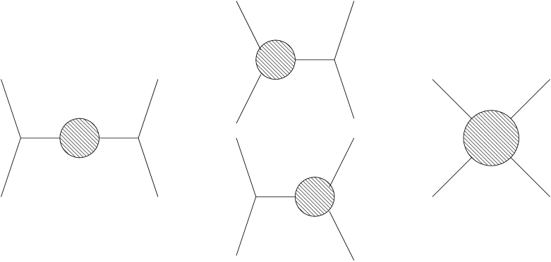
FIG. 1.: One particle irreducible parts in a general $2\to 2$ process.

FIG. 2.: Allowed domain in the $(\delta_{z},\delta_{\gamma})$ plane, without $A_{LR,\mu}$.

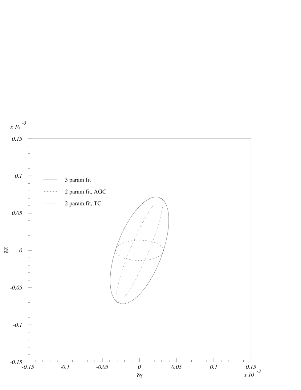
FIG. 3.: Allowed domain in the $(\delta_{z},\delta_{\gamma})$ plane, with $A_{LR,\mu}$.

FIG. 4.: Allowed domain in the $(\delta_{s},\delta_{\gamma})$ plane, without $A_{LR,\mu}$.

FIG. 5.: Allowed domain in the $(\delta_{s},\delta_{\gamma})$ plane, with $A_{LR,\mu}$.

FIG. 6.: Allowed domain in the $(\delta_{z},\delta_{s})$ plane, without $A_{LR,\mu}$.

FIG. 7.: Allowed domain in the $(\delta_{z},\delta_{s})$ plane, with $A_{LR,\mu}$.

FIG. 8.: Projection of the three dimensional ellipse in $(\delta_{z},\delta_{s},\delta_{\gamma})$ space onto the three coordinate planes. Without $A_{LR,\mu}$. The dashed, dot-dashed and dotted stripes are the independent $1\sigma$ regions for $\sigma_{\mu}$, $\sigma_{5}$ and $A_{LR,\mu}$ respectively.

FIG. 9.: Projection of the three dimensional ellipse in $(\delta_{z},\delta_{s},\delta_{\gamma})$ space onto the three coordinate planes. With $A_{LR,\mu}$. The dashed, dot-dashed and dotted stripes are the independent $1\sigma$ regions for $\sigma_{\mu}$, $\sigma_{5}$ and $A_{LR,\mu}$ respectively.

FIG. 10.: Allowed regions in the $(f_{DW},f_{DB})$ plane. With and without $A_{LR,\mu}$.

FIG. 11.: Allowed regions in the $(x_{V},x_{A})$ plane; $x_{i}=F_{i}^{2}/M_{i}^{4}$. With and without $A_{LR,\mu}$.

REFERENCES

- [1] Opportunities and Requirements for Experimentation at a Very High Energy Collider, SLAC-329(1928); Proc. Workshops on Japan Linear Collider, KEK Reports, 90-2, 91-10 and 92-16; P.M. Zerwas, DESY 93-112, Aug. 1993; Proc. of the Workshop on Collisions at 500 GeV: The Physics Potential, DESY 92-123A,B,(1992), C(1993), D(1994), E(1997) ed. P. Zerwas. E. Accomando et al. Phys. Rep. (1) 1998.
- [2] M.E. Peskin, T. Takeushi, Phys. Rev. Lett. (1990) 964.
- [3] G. Altarelli and R. Barbieri, Phys. Lett. (1991) 161.
- [4] M. Beccaria, F. M. Renard, S. Spagnolo, C. Verzegnassi, Bounds on universal new physics effects from fermion-antifermion production at LEP2, to appear on Los Alamos preprint server hep-ph.
- [5] F.M. Renard and C. Verzegnassi, Phys. Rev. (1995) 1369, Phys. Rev. (1996) 1290.
- [6] M. Beccaria, P. Ciafaloni, D. Comelli, F. Renard, C. Verzegnassi Eur. Phys. Jour. (1999) 331.
- [7] G. Degrassi and A. Sirlin, Nucl. Phys. B383, 73 (1992); Phys. Rev. D46, 3104 (1992).
- [8] K. Hagiwara, S. Ishihara, R. Szalapski and D. Zeppenfeld, Phys. Rev. D48, 2182 (1993).
- [9] A. Blondel, F. M. Renard, L. Trentadue and C. Verzegnassi, Phys. Rev. D54, 5567 (1996).
- [10] R. S. Chivukula, F. M. Renard and C. Verzegnassi, Phys. Rev. D57, 2760 (1998).
- [11] F. M. Renard and C. Verzegnassi, Phys. Rev. D55, 4370 (1997).
- [12] E. Eichten, K. Lane, M. Peskin, Phys. Rev. Lett. 50, 811 (1983).
- [13] J. Hewett, Phys. Rev. Lett. 82, 4765 (1999).