Calculation of Power Corrections to Hadronic Event Shapes of Tagged $b$ Events

Abstract:

We compute power corrections to mean values of hadronic event shapes — the thrust and the $C$ parameter — of tagged $b$ quark events in electron positron annihilation, using the dispersive approach. We find that the leading power corrections are of the same type of $1/Q$ corrections as for event shapes in the massless case, with the same non-perturbative coefficient times a perturbatively calculable mass-dependent coefficient. The effect of the mass correction in the power correction is to reduce the latter by 10–30 % for tagged $b$ events, for centre-of-mass energies ranging from the $Z^{0}$ peak down to 20 GeV.

1 Introduction

In recent years the idea of an infrared-regular effective strong coupling at low scales (the strong coupling ‘freezing’ [1] or, more rigorously, the ‘dispersive approach’ of Dokshitzer, Marchesini and Webber [2]) has been employed for estimating hadronization corrections to various hadronic event shapes, using perturbative calculations [3, 4, 5, 6, 7]. These corrections arise in the form of power corrections of order 1/$Q^{p}$, where $Q$ is the centre-of-mass energy. Although the magnitude of the correction cannot be predicted by perturbative means, the power $p$ and the relative coefficients among different observables can be calculated using the assumption of infrared freezing. This universality hypothesis has proved to give a phenomenologically fairly consistent picture of power corrections [8, 9, 10, 11, 12, 13], and the same results could be derived using a different method, the so-called renormalon approach [14, 15].

In this letter we explore a further check of the universality picture. Assuming the flavour independence of gluon radiation off quarks, the analytic structure of the strong coupling in the infrared, defined in an appropriate way, should not depend on the masses of the quarks, which radiate the gluon. Therefore, in the calculation of the power corrections to hadronic event shapes of tagged $b$ events, the mass of the heavy quark enters in a completely perturbative manner. One may expect that the leading mass correction could be $m_{b}/Q$ times the leading power correction ($m_{b}$ being the heavy-quark mass) with some calculable coefficient. If this coefficient is several times unity, then the mass corrections in the power corrections are expected to be significant enough to be a measurable effect.

A similar problem has already been considered by Nason and Webber in calculating non-perturbative corrections to heavy-quark fragmentation in $e^{+}e^{-}$ annihilation [16]. Although the calculations are very similar, there is an essential difference in the results: for the fragmentation function there is a 1/$m_{b}$ power correction, while for tagged events shapes there are mass corrections to the magnitude of the leading 1/$Q^{p}$ power correction, which, however, vanish smoothly in the massless limit.

Estimating the mass corrections in the power correction may be interesting from another point of view, too. Recently, next-to-leading order calculations of three-jet quantities in electron positron annihilation have been performed in which quark mass effects have been taken into account explicitly [18, 17, 19]. Using this theoretical input and the value of the $b$-quark mass, the flavour independence of the strong interactions was demonstrated by determining the ratio of strong couplings, $\alpha_{s}^{b}$/$\alpha_{s}^{uds}$ [20, 21]. One can turn around the argument and, assuming flavour independence, the $b$-quark mass can be measured from the sensitivity of three-jet event shapes to mass effects [22, 23, 24]. Such a measurement requires an estimate of hadronization corrections. The traditional way of obtaining such estimates is by Monte Carlo event generators [25, 26]. Those programs use the heavy-quark mass as input. As a result, the estimate of hadronization corrections brings a significant systematic error into the measurement of $m_{b}$. For taking into account the hadronization correction in a different way, the simple formulae of power corrections presented in this paper can easily be incorporated in a fit to the $b$-quark mass, which would hopefully result in a more stringent mass measurement.

As mentioned above, the presence of the quark mass appears only in the perturbative calculation. Therefore, the calculations that lead to the appearance of the Milan factor in the power corrections [5] can also be performed in the presence of the quark mass, resulting in a mass-dependent Milan factor. In this paper we make only the first step and calculate that part of power corrections to the mean value of two $e^{+}e^{-}$ event shapes, the thrust and the $C$ parameter, which was termed ‘naive contribution’ in Ref. [5].

2 The dispersive approach

In employing the dispersive approach of Ref. [2] one starts with assuming the validity of the following dispersion relation for the strong coupling:

$$\alpha_{s}(k^{2})=-\int_{0}^{\infty}\!\frac{{\rm d}\mu^{2}}{\mu^{2}+k^{2}}\,\rho_{s}(\mu^{2})\>,\qquad\rho_{s}(\mu^{2})=-\frac{1}{2\pi{\rm i}}{\rm Disc}\left\{\alpha_{s}(-\mu^{2})\right\}\>.$$ (1)

Further, it is also assumed that similarly to QED, the dominant effect of the running of $\alpha_{s}$ on some QCD observable $F$ may be represented in terms of the spectral function $\rho_{s}(\mu^{2})$ and a characteristic function ${\cal F}(\mu^{2})$:

$$F=\alpha_{s}(0)\,{\cal F}(0;\ldots)+\int_{0}^{\infty}\!\frac{{\rm d}\mu^{2}}{\mu^{2}}\,\rho_{s}(\mu^{2})\,{\cal F}(\mu^{2};\ldots)$$ (2)

$$\quad=\int_{0}^{\infty}\!\frac{{\rm d}\mu^{2}}{\mu^{2}}\,\rho_{s}(\mu^{2})\,\left[{\cal F}(\mu^{2};\ldots)-{\cal F}(0;\ldots)\right]\>,$$ (3)

where we used Eq. (1) to express $\alpha_{s}$(0). The characteristic funtion ${\cal F}(\mu^{2};\ldots)$ is a function of dimensionless ratios of $\varepsilon\equiv\mu^{2}/Q^{2}$, $\rho\equiv 4\,m_{b}^{2}/Q^{2}$, where $m_{b}$ is the heavy-quark mass and $\{y\}$, the collection of any further relevant dimensionless parameters, e.g. the jet shape $S$ in our present considerations. We obtain ${\cal F}$ by computing the one-loop graphs, corresponding to the physical process under consideration, with a non-zero gluon mass $\varepsilon\neq 0$, and dividing by $\alpha_{s}$:

$${\cal F}(\varepsilon;\rho,S)=\int\!{\rm d}\Phi(\{x_{i}\};\rho,\varepsilon)\,{\cal M}(\{x_{i}\};\rho,\varepsilon)\,S(\{x_{i}\};\rho,\varepsilon)\>,$$ (4)

where ${\rm d}\Phi(\{x_{i}\};\rho,\varepsilon)$ denotes the phase space in terms of the independent variables $\{x_{i}\}$, ${\cal M}$ is the proper squared amplitude divided by $\alpha_{s}$, and $S$ stands for the event shape variable. Introducing the effective coupling $\alpha_{\rm eff}(\mu^{2})$, defined in terms of the spectral function by

$$\rho_{s}(\mu^{2})=\mu^{2}\frac{{\rm d}\alpha_{\rm eff}}{{\rm d}\mu^{2}}\>,$$ (5)

we can integrate Eq. (3) by parts to obtain

$$F=\int_{0}^{\infty}\!\frac{{\rm d}\mu^{2}}{\mu^{2}}\,\alpha_{\rm eff}(\mu^{2})\,\dot{{\cal F}}(\mu^{2})=\int_{0}^{\infty}\!\frac{{\rm d}\varepsilon}{\varepsilon}\,\alpha_{\rm eff}(Q^{2}\varepsilon)\,\dot{{\cal F}}(\varepsilon)\>,$$ (6)

where

$$\dot{{\cal F}}(\varepsilon)=-\varepsilon\frac{{\rm d}{\cal F}}{{\rm d}\varepsilon}\>.$$ (7)

Using the definition Eq. (5) and the dispersion relation Eq. (1), we can deduce that in the perturbative domain, $\alpha_{s}\ll 1$, the standard and effective couplings are approximately the same [2]:

$$\alpha_{\rm eff}(\mu^{2})=\alpha_{s}(\mu^{2})+\mathrm{O}(\alpha_{s}^{3})\>.$$ (8)

Thus we may interpret $\alpha_{\rm eff}$ as an effective coupling that extends the physical perturbative coupling into the non-perturbative domain. If the effective coupling has a non-perturbative component $\delta\alpha_{\rm eff}(\mu^{2})$, with support limited to low values of $\mu^{2}$, the corresponding contribution to $F$,

$$\delta F=\int_{0}^{\infty}\!\frac{{\rm d}\varepsilon}{\varepsilon}\,\delta\alpha_{\rm eff}(Q^{2}\varepsilon)\,\dot{{\cal F}}(\varepsilon)\>,$$ (9)

will have a $Q^{2}$ dependence determined by the small-$\varepsilon$ behaviour of $\dot{{\cal F}}$.

We shall be interested in the leading power behaviour of $\delta F$, which will be called the leading power correction to $F$,

$$\delta F=F^{\rm pow}+O\Big{(}1/Q^{p}\Big{)}\>.$$ (10)

In order to determine $F^{\rm pow}$, we recall that power-suppressed contributions to $\delta F$ can arise from only those terms in ${\cal F}$ that are non-analytic at $\varepsilon=0$ [2]. Therefore, the leading power correction $F^{\rm pow}$ will be obtained from the leading non-analytic term at $\varepsilon=0$ in $\dot{{\cal F}}$, which we denote by $C_{F}\,\delta{\cal F}/2\pi$.

3 Calculations

In calculating the function $\delta{\cal F}$ for the $e^{+}e^{-}$$\rightarrow$$\>Q{\bar{Q}}g$ event shapes, we find three sources of quark-mass dependence: (i) restriction of phase space; (ii) mass corrections in the matrix element; (iii) mass corrections in the definition of the event shape. The double differential cross section for the production of a massive quark antiquark pair and a massive gluon given in terms of the scaled quark, antiquark and gluon energies, $x$, $\bar{x}$ and $x_{g}=2-x-\bar{x}$ was derived in Ref. [16]. This cross section is an analytic function of the gluon mass and, therefore, in calculating $\delta{\cal F}$, the $\varepsilon$-dependent terms can be dropped completely. In the case of the vector current contribution the cross section for zero gluon mass is given by

$$\frac{1}{\sigma_{V}}\frac{{\rm d}\sigma_{V}}{{\rm d}x\,{\rm d}\bar{x}}=\frac{C_{F}}{\beta}\frac{\alpha_{s}}{2\pi}\Bigg{[}\frac{-\lambda(x^{2}-\rho,\bar{x}^{2}-\rho,x_{g}^{2})}{8\,(1-x)^{2}\,(1-\bar{x})^{2}}$$ (11)

$$\qquad\qquad\qquad\qquad+\frac{1}{1+{\textstyle\frac{1}{2}}\rho}\,\left(\frac{1}{(1-x)^{2}}+\frac{1}{(1-\bar{x})^{2}}\right)\Bigg{]}\>;$$

for the axial vector current contribution we have

$$\frac{1}{\sigma_{A}}\frac{{\rm d}\sigma_{A}}{{\rm d}x\,{\rm d}\bar{x}}=\frac{C_{F}}{\beta}\frac{\alpha_{s}}{2\pi}\Bigg{[}\frac{-\lambda(x^{2}-\rho,\bar{x}^{2}-\rho,x_{g}^{2})}{8\,(1-x)^{2}\,(1-\bar{x})^{2}}$$ (12)

$$\qquad\qquad\qquad\qquad+\frac{1}{1-\rho}\,\left(\frac{1}{(1-x)^{2}}+\frac{1}{(1-\bar{x})^{2}}+\frac{\rho}{2}\,\frac{x_{g}^{2}}{(1-x)\,(1-\bar{x})}\right)\Bigg{]}\>,$$

where $\beta=\sqrt{1-\rho}$ is the quark velocitey and $\lambda(x,y,z)=x^{2}+y^{2}+z^{2}-2\,x\,y-2\,y\,z-2\,z\,x$. In Eqs. (11) and (12)

$$\sigma_{V}=\sigma_{0}\,\left(1+{\textstyle\frac{1}{2}}\,\rho\right)\,\beta\>,\qquad$$ (13)

and

$$\sigma_{A}=\sigma_{0}\,\left(1-\rho\right)\,\beta$$ (14)

are the Born cross sections for heavy-quark production by a vector and an axial vector current respectively, $\sigma_{0}$ being the massless quark Born cross section. The corresponding phase space was also given in Ref. [16]:

$${\rm d}\Phi(x,\bar{x};\varepsilon,\rho)={\rm d}x\,{\rm d}\bar{x}\,\Theta\Big{(}-{\textstyle\frac{1}{8}}\,\lambda(x^{2}-\rho,\bar{x}^{2}-\rho,x_{g}^{2}-4\varepsilon)\Big{)}\,$$ (15)

The phase-space boundary in this equation gives $x_{-}\leq\bar{x}\leq x_{+}$, where

$$x_{\pm}=\frac{(2-x)(1-x-\varepsilon+{\textstyle\frac{1}{2}}\,\rho)\pm\sqrt{(x^{2}-\rho)[(1-x-e)^{2}-\varepsilon\,\rho]}}{2\,(1-x)+{\textstyle\frac{1}{2}}\,\rho}$$ (16)

and

$$\sqrt{\rho}\leq x\leq 1-e-\sqrt{\varepsilon\,\rho}\>.$$ (17)

For large values of the gluon momentum the phase-space boundary does not yield leading non-analytic contributions in $\varepsilon$. Therefore, the leading non-analytic contribution to $\delta{\cal F}$ comes from the soft-gluon emission region [2, 16], where both the matrix elements, in Eqs. (11) and (12), and the phase space, in Eq. (15), can be expanded in $x_{g}=y+\bar{y}\simeq\sqrt{\varepsilon}$. This expansion for the cross section formulae results in

$$\frac{1}{\sigma_{V,A}}\frac{{\rm d}\sigma_{V,A}}{{\rm d}y\,{\rm d}\bar{y}}\approx\frac{C_{F}}{\beta}\frac{\alpha_{s}}{2\pi}\left[\frac{2}{y\,\bar{y}}-\frac{\rho}{2}\,\frac{(y+\bar{y})^{2}}{y^{2}\,\bar{y}^{2}}\right]$$ (18)

both for vector and axial vector current contributions, where $y=1-\bar{x}$ and $\bar{y}=1-x$. The lower boundary of the phase space in $x_{g}=y+\bar{y}\simeq\sqrt{\varepsilon}$ region is approximated as follows:

$$-\frac{1}{8}\,\lambda(x^{2}-\rho,\bar{x}^{2}-\rho,x_{g}^{2}-4\varepsilon)\approx 2\,y\,\bar{y}-\frac{\rho}{2}\,(y+\bar{y})^{2}-2\,\varepsilon\,(1-\rho)=0\>.$$ (19)

Thus, to obtain $\delta{\cal F}$ for mean values of event shapes, we have to calculate the following integral

$$\!\!\!\!\!\!\delta{\cal F}=-\,\frac{\varepsilon}{\beta}\,\frac{{\rm d}}{{\rm d}\varepsilon}\int\!{\rm d}y\,{\rm d}\bar{y}\,\Theta(y-\sqrt{\varepsilon\rho})\,\Theta(\bar{y}-\sqrt{\varepsilon\rho})\,\Theta(1-\rho/2-y-\bar{y})$$ (20)

$$\qquad\qquad\qquad\;\times\Theta(4\,y\,\bar{y}-\rho\,(y+\bar{y})^{2}-4\,\varepsilon\,(1-\rho))$$

$$\qquad\qquad\qquad\;\times\frac{2}{y\,\bar{y}}\,\left(1-\frac{\rho}{4}\,\frac{(y+\bar{y})^{2}}{y\,\bar{y}}\right)S(y,\bar{y};\rho,\varepsilon)\>.$$

In this equation, the exact form of the upper boundary does not influence those non-analytic terms that give the leading power correction.

The mass corrections in the physical quantity introduce an observable-dependent, but perturbatively calculable mass dependence. As simple application of formula (20), we consider two event shapes, the $C$ parameter and the thrust $T$. The $C$ parameter [27] is derived from the eigenvalues of the infrared-safe momentum tensor

$$\theta^{ij}=\sum_{a}\frac{p_{a}^{i}p_{a}^{j}}{|\vec{p}_{a}|}\bigg{/}\sum_{a}|\vec{p}_{a}|,$$ (21)

where the sum on $a$ runs over all final-state hadrons and $p_{a}^{i}$ is the $i$th component of the three-momentum $\vec{p}_{a}$ of hadron $a$ in the c.m. system. The tensor $\theta$ is normalized to have unit trace. In terms of the eigenvalues $\lambda_{i}$ of the $3\times 3$ matrix $\theta$, the global shape parameter $C$ is defined as

$$C=3\,(\lambda_{1}\lambda_{2}+\lambda_{2}\lambda_{3}+\lambda_{3}\lambda_{1})\>.$$ (22)

The thrust [28] is given by

$$T=\max_{\vec{n}_{T}}\left(\frac{\sum_{a}|\vec{p}_{a}\cdot\vec{n}_{T}|}{\sum_{a}|\vec{p}_{a}|}\right),$$ (23)

where the sum runs over all final-state particles and the thrust axis ${\vec{n}_{T}}$ is chosen to maximize the expression. For three partons in the final state, the thrust can be written as [29]

$$T=2\frac{\max\{|\vec{p}_{1}|,|\vec{p}_{2}|,|\vec{p}_{3}|\}}{\sum_{a}|\vec{p}_{a}|}\>.$$ (24)

Instead of the thrust, we shall consider its deviation from unity, $t=1-T$.

For these two event shapes the contribution of the non-perturbative gluon will just add to that of the underlying perturbative event (contribution of many soft perturbative gluons), and the power correction based on the presence of just a single non-perturbative gluon will remain valid [13]. This argument can be used independently of the mass of the leading quark pair. As discussed in Ref. [5], the ‘naive contribution’ to the mean value of the $C$ parameter is obtained from Eq. (22) in the soft-gluon approximation, with gluon mass set to zero. The corresponding formula with non-zero quark masses is the following:

$$C(y,\bar{y};\rho)\approx\frac{6}{\beta^{3}}\,\frac{y\,\bar{y}}{y+\bar{y}}\,\left(1-\frac{\rho}{4}\,\frac{(y+\bar{y})^{2}}{y\,\bar{y}}\right)\>.$$ (25)

Similarly, we need only the leading term in the soft-gluon expansion of the function $t(y,\bar{y};\rho)$ with the gluon mass neglected,

$$t(y,\bar{y};\rho)\approx\frac{1}{2}\,\left(\frac{y+\bar{y}}{\sqrt{1-\rho}}-\frac{1}{1-\rho}\,\Big{[}(\bar{y}-y)\,\Theta(\bar{y}-y)+(y-\bar{y})\,\Theta(y-\bar{y})\Big{]}\right)\>.$$ (26)

To perform the integrations in Eq. (20) we introduce polar coordinates, $y=r\,\cos\phi$, $\bar{y}=r\,\sin\phi$. In terms of the variables $r$ and $\phi$

$${\rm d}\Phi(\varepsilon)=r\,{\rm d}r\,{\rm d}\phi\,\Theta(\phi-\delta)\,\Theta({\textstyle\frac{1}{2}}\pi-\delta-\phi)\,\Theta(r_{+}(\phi)-r)\,\Theta(r-r_{-}(\phi,\varepsilon))\>,$$ (27)

where

$$r_{+}(\phi)=\frac{(1+\sin 2\delta)^{-1}}{\sqrt{1+\sin 2\phi}}\>,\quad r_{-}(\phi,\varepsilon)=\sqrt{\frac{2\,\varepsilon\,(1-\sin 2\delta)}{\sin 2\phi-\sin 2\delta}}\>,\quad\sin 2\delta=\frac{\rho}{2-\rho}\>.$$ (28)

The $r$ integral is trivial and the integral over $\phi$ can be performed after making the shift $\phi\rightarrow\phi-\pi/4$. After performing the differentiation in Eq. (20), for the $C$ parameter, $S=C$, we obtain

$$\delta{\cal F}^{(C)}=6\pi\,\sqrt{\varepsilon}\,\frac{1}{\beta}\,\left(\frac{1}{1+\sqrt{\rho}}-\frac{\sqrt{\rho}}{2}\right)$$ (29)

$$\qquad\quad=6\pi\,\sqrt{\varepsilon}\,\left(1-\frac{3}{2}\,\sqrt{\rho}+\mathrm{O}(\rho)\right)\>.$$ (30)

From the expansion at small values of $\rho$, we see that our formula reproduces the known zero mass result [1]. In the case of thrust, $S=t$, one finds

$$\delta{\cal F}^{(t)}=\sqrt{\frac{\varepsilon}{\rho}}\left(\pi\,\beta-\frac{1}{1-\rho}\Big{(}\alpha_{+}+\alpha_{-}-2\,\sqrt{\rho\,(1-\rho)}\Big{)}\right)\>,$$ (31)

where

$$\alpha_{\pm}=\arctan\frac{2-\rho\pm\sqrt{2}}{\sqrt{\rho\,(1-\rho)}}\>.$$ (32)

Expanding $\delta{\cal F}^{(t)}$ in $\rho$ we find

$$\delta{\cal F}^{(t)}=4\,\sqrt{\varepsilon}\,\left(1-\frac{3\pi}{8}\sqrt{\rho}+\mathrm{O}(\rho)\right)\>,$$ (33)

which shows that the apparent $\sqrt{\varepsilon/\rho}$ behaviour in Eq. (31) is in fact a $\sqrt{\varepsilon}$ behaviour with multiplicative mass corrections that are regular for vanishing quark mass. Setting $\rho=0$, we find agreement with the known zero-mass result [1].

In Fig. 1 we plotted the functions $\dot{{\cal F}}(\varepsilon)$ in Eq. (7), obtained from numerical integration for representative values of $\rho$, with ${\cal F}$ as given in Eq. (4), but with $S$ taken in the soft-gluon approximation (Eq. (25) for $S=C$ in Fig. 1a and Eq. (26) for $S=t$ in Fig. 1b). In the same figure, the solid lines show the analytic results $\delta{\cal F}^{(C)}$, Eq. (29), and $\delta{\cal F}^{(t)}$, Eq. (31). We clearly see the leading $\sqrt{\varepsilon}$ behaviour for small values of $\varepsilon$ together with the correct quark-mass dependence.

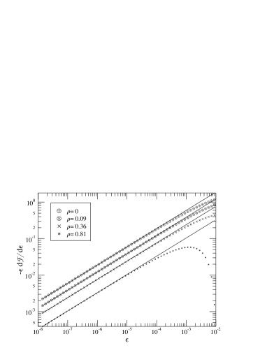
Figure 1: Derivative of the characteristic function for the mean value of the (a) $C$ parameter (b) $1-T$ for values of $\rho=0$, 0.09, 0.36, 0.81.

Having calculated the derivative of the characteristic functions for the various event shapes, we can use Eq. (10) to obtain the power correction $F^{\rm pow}$. Following Ref. [2], we introduce the moment integral

$$A_{2p}=\frac{C_{F}}{2\pi}\int_{0}^{\infty}\!\frac{{\rm d}\varepsilon}{\varepsilon}\,\varepsilon^{p}\,\delta\alpha_{\rm eff}(\varepsilon Q^{2})\>.$$ (34)

In terms of this non-perturbative parameter, the ‘naive contribution’ to the power corrections to the mean value of $C$ and $t$ are given by the $p={\textstyle\frac{1}{2}}$ moment of $\delta\alpha_{\rm eff}$ as

$$\langle C\rangle^{\rm pow}=6\,\pi\,\frac{A_{1}}{Q}\,\left(1-3\,\frac{m_{b}}{Q}+\mathrm{O}\left(\frac{m_{b}^{2}}{Q^{2}}\right)\right)$$ (35)

and

$$\langle t\rangle^{\rm pow}=4\,\frac{A_{1}}{Q}\,\left(1-\frac{3\pi}{4}\,\frac{m_{b}}{Q}+\mathrm{O}\left(\frac{m_{b}^{2}}{Q^{2}}\right)\right)\>,$$ (36)

with the same value of the moment integral as phenomenologically deduced from untagged samples. To obtain these leading mass corrections, valid for small values of the tagged-quark mass, we used Eqs. (30) and (33). These results show that at LEPI energies the mass correction reduces the magnitude of the power correction by about 10 % for the mean value of the $C$ parameter and by about 7 % for the mean value of $t$ (with $m_{b}$ taken to be the $\overline{{\rm MS}}$ mass at the centre-of-mass energy).

A two-loop analysis of power corrections to event shapes in the massless-quark case revealed that there is some freedom in the definition of the ‘naive contribution’. With a different definition for this term, the other two (‘inclusive’ and ‘non-inclusive’) contributions change in such a way that the sum of the three terms remains unambiguous. The universal result can be summarized by a simple multiplicative correction factor, the so-called Milan factor [5]. A two-loop calculation with mass effects taken into account would modify our results in Eqs. (35) and (36) in two ways. On the one hand, these equations would acquire an overall Milan factor of 1.5 and on the other the coefficients in front of the $m_{b}/Q$ corrections would change. For the rest of this paper, we shall neglect the latter modification, but shall include the Milan factor.

4 Merging perturbative and non-perturbative contributions

Once we have the leading power correction, we have to combine it with the perturbative prediction for the same physical quantity to obtain the full theoretical prediction:

$$F(Q)=F^{\rm pert}(Q)+F^{\rm pow}(Q)\>.$$ (37)

The two contributions are separately ill-defined because the perturbative part is given by an expansion that is factorially divergent, while in the power correction, the non-perturbative part of the effective coupling $\delta\alpha_{\rm eff}$ contains an ill-defined all-order subtraction of the pure perturbative part off the full effective coupling $\alpha_{\rm eff}$. The sum of the two contributions is finite. At fixed order in perturbation theory they should be merged in such a way that the terms that would grow factorially in an all-order result cancel order by order. We follow the prescription of Ref. [5] for this merging, where the moment integral $A_{1}$ was approximated with the same integral up to an infrared scale $\mu_{\rm I}$,

$$A_{1}\simeq\frac{2\,C_{F}}{\pi^{2}}\int_{0}^{\mu_{\rm I}}\!{\rm d}k\,\left[\alpha_{s}(k)-\alpha_{s}^{\rm pert}(k)\right]\>.$$ (38)

In this equation the integrand is the non-perturbative component of the strong coupling, i.e. the difference of the strong coupling $\alpha_{s}$ as given by Eq. (1) and the perturbative coupling $\alpha_{s}^{\rm pert}$. Above the infrared scale $\mu_{\rm I}$, this non-perturbative coupling is assumed to give negligible contribution to the moment integral (see Eq. (8) and the following paragraph).

The integral of the strong coupling in Eq. (38) can be expressed in terms of a phenomenological parameter $\alpha_{0}$,

$$\int_{0}^{\mu_{\rm I}}\!{\rm d}k\,\alpha_{s}(k)\equiv\mu_{\rm I}\,\alpha_{0}(\mu_{\rm I})\>.$$ (39)

The value of this parameter depends on the infrared matching scale. For $\mu_{\rm I}=2\,$GeV, fits of event shapes of untagged events gave $\alpha_{0}\simeq 0.5$ [1, 9, 11, 12, 13].

To calculate the integral of the perturbative coupling $\alpha_{s}^{\rm pert}$, we use its one-loop expression given as a geometric series:

$$\frac{\alpha_{s}^{\rm pert}(k)}{2\pi}=\frac{\alpha_{s}^{\rm pert}(Q)}{2\pi}\sum_{\ell=0}^{\infty}\left(\frac{\alpha_{s}^{\rm pert}(Q)}{2\pi}\,\beta_{0}^{(4)}\,\ln\frac{Q}{k}\right)^{\ell}\>,$$ (40)

where $\beta_{0}^{(4)}$ is the one-loop beta function

$$\beta_{0}^{({N_{\rm f}})}=\frac{11}{3}\,C_{A}-\frac{2}{3}\,{N_{\rm f}}\>,$$ (41)

for ${N_{\rm f}}=4$ light fermion flavours, and $\alpha_{s}^{\rm pert}(Q)$ is a four-flavour perturbative coupling in the physical (CMW) renormalization scheme [31].

For the practically interesting cases the perturbative prediction for the event shape the perturbative prediction $F^{\rm pert}$ is known to second order in $\alpha_{s}$,

$$F^{\rm pert}(Q;2)=\frac{\alpha_{s}^{\overline{{\rm MS}}}(Q)}{2\,\pi}\,B(m_{b},Q)+\left(\frac{\alpha_{s}^{\overline{{\rm MS}}}(Q)}{2\,\pi}\right)^{2}\,C(m_{b},Q)+\mathrm{O}\left((\alpha_{s}^{\overline{{\rm MS}}}(Q))^{3}\right)\>,$$ (42)

with Born and correction coefficients, $B(m_{b},Q)$ and $C(m_{b},Q)$ respectively, calculated in the $\overline{{\rm MS}}$ scheme at scale $Q$, and $\alpha_{s}^{\overline{{\rm MS}}}(Q)$ is the four-flavour strong coupling defined in the $\overline{{\rm MS}}$ renormalization scheme. In such cases the summation in Eq. (40) should be truncated at O($\alpha_{s}^{2}$), that is at $\ell=1$. Then the integral of the perturbative coupling in Eq. (38) gives

$$\mu_{\rm I}\,\left[\frac{\alpha_{s}^{\rm pert}(Q)}{2\,\pi}+\left(\frac{\alpha_{s}^{\rm pert}(Q)}{2\,\pi}\right)^{2}\beta_{0}^{(4)}\,\left(\ln\frac{Q}{\mu_{\rm I}}+1\right)\right]\>.$$ (43)

In order to use the $\overline{{\rm MS}}$ coupling everywhere in the final result, one has to make the shift

$$\alpha_{s}^{\rm pert}\rightarrow\alpha_{s}^{\overline{{\rm MS}}}\,\left(1+K\,\frac{\alpha_{s}^{\overline{{\rm MS}}}}{2\,\pi}\right)$$ (44)

in Eq. (43), with $K$ defined as

$$K=C_{A}\left(\frac{67}{18}-\frac{\pi^{2}}{6}\right)-\frac{5}{9}\,{N_{\rm f}}\>,\quad{N_{\rm f}}=4\>.$$ (45)

The coupling in the definition of the non-perturbative parameter $\alpha_{0}$ is the physical coupling; therefore, the value of $\alpha_{0}$ does not depend on the chosen scheme.

Collecting the various contributions, for the event shape $S(=t$, or $C)$ we find

$$F^{(S)}(Q)=\bar{\alpha}_{s}\,B+\bar{\alpha}_{s}^{2}\,C$$ (46)

$$\qquad\qquad+\frac{2}{\pi}{\cal M}\,\frac{2C_{F}}{\sqrt{\varepsilon}}\,\delta{\cal F}^{(S)}(\rho,\varepsilon)\,\frac{\mu_{\rm I}}{Q}\left(\bar{\alpha}_{0}-\bar{\alpha}_{s}-\bar{\alpha}_{s}^{2}\left[\beta_{0}^{(4)}\,\left(\ln\frac{Q}{\mu_{\rm I}}+1\right)+K\right]\right)\>,$$

where $\bar{\alpha}_{s}\equiv\alpha_{s}^{\overline{{\rm MS}}}(Q)/2\pi$ for ${N_{\rm f}}=4$ flavours and $\bar{\alpha}_{0}\equiv\alpha_{0}/2\pi$. In order to use the standard ${N_{\rm f}}=5$ flavour $\overline{{\rm MS}}$ strong coupling, we have to make the shift

$$\bar{\alpha}_{s}\rightarrow\bar{\alpha}_{s}+\frac{2}{3}\,\bar{\alpha}_{s}^{2}\,\ln\left(\frac{m_{b}}{Q}\right)\>.$$ (47)

We could make a more sophisticated description of the heavy-quark threshold in the running coupling (see Refs. [32, 33]), but the usual centre-of-mass energy for event shapes being far from the threshold, the difference is negligible. For instance, using the prescription of Ref. [33] changes the physical prediction $F^{(S)}(Q)$ by less than 1 % at $Q=20\,$GeV and by about $0.1\,\%$ at the $Z^{0}$ peak. The renormalization scale dependence of this result can be studied in the usual way. To show the effect of the mass correction, we plot $F^{(S)}$ for $S=C$ in Fig. 2a and for $S=t$ in Fig. 2b for $\mu_{\rm I}=2\,$GeV, $\alpha_{0}=0.5$ and the world average of the strong coupling at the $Z^{0}$ peak, $\alpha_{s}(M_{Z})=0.119$ [34]. The solid lines show the results for the central value of the $\overline{{\rm MS}}$ $b$-quark mass at the given hard scattering scale run from $m_{b}(m_{b})=4.3\,$GeV [32]. The dotted line is the next-to-leading order perturbative prediction, with mass effects included, and the dashed lines represent the result when mass effects are present in the perturbative prediction plus power corrections without mass effects. The perturbative coefficients $B$ and $C$ were obtained using the zbb4 program [35]. We can observe that the mass effect in the power correction in tagged $b$ samples is important for centre-of-mass energies below about 45 GeV.

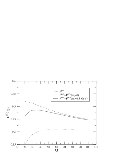
Figure 2: Mean value of (a) the $C$ parameter and (b) $1-T$, where $T$ is the thrust. Dotted: next-to-leading order perturbative result, dashed: perturbative + power correction without mass effect, solid: perturbative + power correction with mass effect.

If we compare our results for the power corrections of tagged $b$ events to the hadronization corrections obtained using Monte Carlo programs, we find significantly smaller corrections from our model. For instance, the double ratio $H_{b/l}^{(s)}=H^{(S)}_{b}/H^{(S)}_{l}$, where $H^{(S)}_{x}$ is the hadron level value divided by the parton level value for event shape $S$ and for the quark flavour $x$ (heavy, or light), was determined in Ref. [24] for events in $Z^{0}$ decays using JETSET parton shower model together with the Lund string fragmentation model. In this model the mass effects are introduced only by kinematic constraints to the phase space at each parton branching in the shower evolution. Table 1 shows the values obtained for $H_{b/l}^{(s)}$ using the two models.

$S$	JETSET	Disp. model
$C$	1.175	1.000
$t$	1.142	1.001

Table 1: Comparison of hadronization corrections obtained using JETSET and from the dispersive model via the double ratios $H_{b/l}^{(C)}$ and $H_{b/l}^{(t)}$.

The values for the double ratios obtained from the dispersive approach are very close to 1, indicating that the relative power corrections are very similar in the $b$-tagged and $uds$-tagged samples. The situation is very different for the JETSET estimates. The results, when translated for single ratios of hadronization corrections on the tagged sample $H^{(S)}_{b}$, mean that the hadronization correction from the dispersive approach is about half of that from JETSET. It would be interesting to learn whether or not this difference changes if the mass effects are taken into account in the dynamics of the showering in JETSET, or it is rather due to the different secondary decays of heavy hadrons. The latter case may undermine the usefulness of estimating hadronization corrections from power corrections for tagged $b$ events.

5 Conclusion

In this paper we have calculated the ‘naive contribution’, as defined in Ref. [5], for the power corrections of $b$-tagged event shapes thrust and $C$ parameter in $e^{+}e^{-}$ annihilation. At LEPI energy the explicit analytic formulae predict about 7–10 % reduction of the hadronization correction for the shapes obtained from $b$-tagged samples with respect to the untagged case. This reduction effect will be even more important for $t$-tagged samples at the NLC. For instance, for $m_{t}=175$ GeV and $Q=500$ GeV, we expect the power correction to be about two thirds of the corresponding massless case for the $C$ parameter and $t$.

We also presented predictions for the mean values of the event shapes by merging the perturbative and non-perturbative contributions. The only non-perturbative input in the prediction is the non-perturbative parameter $\alpha_{0}$, taken from fits of theoretical predictions for the mean values of event shapes to those of light primary quark samples. We found that the mass effect in the power correction for tagged $b$ samples is not too profound for centre-of-mass energies above about 45 GeV and is significantly smaller than the hadronization correction predicted by the current version of JETSET, which does not take into account the heavy-quark mass in the dynamics of fragmentation, but includes decays of heavy hadrons. The results may be used directly in heavy-quark mass measurements.

In our view the flavour independence of the strong coupling is a sufficiently weak assumption so that if it is feasible with the dispersive approach to calculate non-perturbative effects in hadronic event shapes, then the primary quark mass effects should be perturbatively calculable. Therefore, our results, once confronted with experiment, can serve as a further check of perturbatively calculable hadronization corrections.