A full Next to Leading Order study of
direct photon pair production in hadronic collisions
B.P. 110, F-74941 Annecy-le-Vieux Cedex, France)
Abstract
We discuss the production of photon pairs in hadronic collisions, from fixed target to LHC energies. The study which follows is based on a QCD calculation at full next-to-leading order accuracy, including single and double fragmentation contributions, and implemented in the form of a general purpose computer program of “partonic event generator” type. To illustrate the possibilities of this code, we present the comparison with observables measured by the WA70 and D0 collaborations, and some predictions for the irreducible background to the search of Higgs bosons at LHC in the channel . We also discuss theoretical scale uncertainties for these predictions, and examine several infrared sensitive situations which deserve further study.
LAPTH-760/99
1 Introduction
The production of pairs of direct photons222The word
“direct” means here that these photons do not result from the decay of
, , at large transverse momentum. Direct photons may be
produced according to two possible mechanisms: either they take part
directly to the hard subprocess, or they result from the fragmentation
of partons themselves produced at high transverse momentum in the
subprocess; see sect. 2. with large invariant mass is the so called
irreducible background for the search of the Higgs boson in the two
photon decay channel in the intermediate mass range GeV GeV at the forthcoming LHC. This background is huge and requires to be
understood and quantitatively evaluated.
Beside this important motivation, this process deserves interest by its own.
The production of such pairs of photons has been experimentally studied in a
large domain of energies, from fixed targets [1, 2, 3]
to colliders [4, 5, 6]. A wide variety of observables has been
measured, such as distributions of invariant mass, azimuthal angle and
transverse momentum of the pairs of photons, inclusive transverse momentum
distributions of each photon, which offer the opportunity to test our
understanding of this process.
The aim of this article is to present a study of diphoton hadroproduction based on a computer code of partonic event generator type. In this code, we account for all contributing processes consistently at next-to-leading order (NLO) accuracy, together with the so called box contribution . This code is flexible enough to accommodate various kinematic or calorimetric cuts. Especially, it allows to compute cross sections for both inclusive and isolated direct photon pairs, for any infrared and collinear safe isolation criterion which can be implemented at the partonic level. This article is organized according to the following outline. In section 2, we remind the basic theoretical ingredients, and present the method used to build the computer code developed for this study. Section 3 is dedicated to the phenomenology of photon pair production. We start with a comparison with fixed target and collider experiments. We then provide some predictions for LHC, together with a discussion of theoretical scale uncertainties. The theoretical discussion about the present day limitations of our code is continued in section 4. There we mention various infrared sensitive situations, which would deserve some more care, and for which the resummation of multiple soft gluon effects would be required, in order to improve the ability of our code to account for such observables. Section 5 gathers our conclusions and perspectives.
2 Theoretical content and presentation of the method
Let us first remind briefly the theoretical level of accuracy and limitations of works prior to the present one, in order to assess the improvements which we introduce. Then we present the method which we used to build our computer code DIPHOX.
2.1 Theoretical content
The theoretical understanding of this process relies on NLO calculations,
initiated in [7]. The leading order contribution to diphoton
reactions is given by the Born level process see for instance Diagram a. The computation of NLO contributions to it
yields corrections coming from the subprocesses , (or ) (or ) and corresponding virtual corrections, see for
example Diagrams b and c.
Yet it also yields the leading order contribution of single fragmentation type
(sometimes called “Bremsstrahlung contribution”), in which one of the photons
comes from the collinear fragmentation of a hard parton produced in the short
distance subprocess, see for example Diagram d. From a physical point of view
such a photon is most probably accompanied by hadrons. From a technical point
of view, a final state quark-photon collinear singularity appears in the
calculation of the contribution from the subprocess . At higher orders, final state multiple collinear singularities
appear in any subprocess where a high parton (quark or gluon)
undergoes a cascade of successive collinear splittings ending up with a
quark-photon splitting. These singularities are factorized to all orders in
according to the factorization property, and absorbed into quark and
gluon fragmentation functions to a photon defined in some arbitrary fragmentation scheme, at some
arbitrary fragmentation scale . When the fragmentation
scale , chosen of the order of the hard scale of the subprocess, is
large compared to any typical hadronic scale GeV, these functions
behave roughly as . Then a power counting argument
tells that these contributions are asymptotically of the same order in
as the Born term . What is
more, given the high gluon luminosity at LHC, the (or )
initiated contribution involving one photon from fragmentation even dominates
the inclusive production rate in the invariant mass range GeV GeV. A consistent treatment of diphoton
production at NLO thus requires that corrections to these
contributions be calculated also, see for example Diagrams e and f. They have
not been incorporated in [7, 8, 9], and we compute them in the
present work.
The calculation of these corrections in their turn yields the leading order
contribution of yet another mechanism, of double fragmentation type, see for
example Diagram g. In the latter case, both photons result from the collinear
fragmentation of a hard parton. In order to present a study of consistent NLO
accuracy, NLO corrections to this double fragmentation contribution, see for
example Diagrams h and i, have to be calculated accordingly. This is also done
in the present article.
We call “two direct” the contribution given by the Born term plus the
fraction of the higher order corrections from which final state collinear
singularities have been subtracted according to the
factorization scheme.
We call “one fragmentation” (“two fragmentation”) the contribution involving
one single fragmentation function (two fragmentation functions) of a parton
into a photon. Let us add one more comment about the splitting into these
three mechanisms. One must keep in mind that this distinction is schematic
and ambiguous. We remind that it comes technically from the appearance of
final state collinear singularities, which are factorized and absorbed into
fragmentation functions at some arbitrary fragmentation scale333More
generally, the definition of the fragmentation functions rely on the choice of
a given factorization scheme, e.g. the scheme in this work.
The fragmentation functions which we use are presented in [10].
. Each of the contributions associated with these three mechanisms thus
depends on this arbitrary scale. This dependence on cancels
only in the sum of the three, so that this sum only is a physical observable.
More precisely, a calculation of these contributions beyond leading order is
required to obtain a (partial) cancellation of the dependence on . Indeed
this cancellation starts to occur between the higher order of the “two direct”
contribution and the leading order of the “one fragmentation” term, and
similarly between the “one-” and “two fragmentation” components respectively.
This is actually one of the first motivations of the present work. Thus, even
though it may be suggestive to compare the respective sizes and shapes of the
separate contributions for a given choice of scale, as will be done in 3.2.1, we emphasize that only their sum is meaningful.
Beyond this, the so-called box contribution through a quark loop is also included, see for
example Diagram j. Strictly speaking it is a NNLO contribution from the point of
view of power counting. However in the range of interest at LHC for the search
of the Higgs boson, the gluon luminosity is so large compared with the quark
and antiquark one, that it nearly compensates the extra powers of ,
so as to yield a contribution comparable with the Born term. For this reason,
it has been included in previous works, and will be in the present one as
well. We define the “direct” contribution as the sum “two direct” + box.
Actually one should notice, firstly, that other NNLO gluon-gluon initiated processes, such as the collinear finite part of have been ignored444The collinear divergent parts of these processes have been already taken into account in the NLO corrections to the “one fragmentation” contribution and leading order “two fragmentation” components respectively., although they could also be large. Secondly one should also even worry about the next correction to the box, because the latter may be quite sizeable. Such a possibility is suggested by the situation occurring to the first correction to the effective vertex , computed in [11], and shown to reach generically about 50 % of the one-loop result. Moreover, this box contribution is the leading order of a new mechanism, whose spurious (factorization and renormalization) scale dependences are monotonic, and only higher order corrections would partly cure this problem and provide a quantitative estimate. This tremendous effort has not been carried out yet, although progresses towards this goal have been achieved recently [12, 13, 14].
2.2 Presentation of the method
In [7], a dedicated calculation was required for each observable. Since then more versatile approaches have been developed, which combine analytical and Monte-Carlo integration techniques [8], [15]. They thus allow the computation of several observables within the same calculation, at NLO accuracy, together with the incorporation of selection/isolation cuts at the partonic level in order to match the various cuts used by the experimental collaborations as faithfully as possible. The studies of [8] and of [9] rely on such an approach. Let us briefly describe the one which we use here.
2.2.1 Phase space slicing and subtraction of long distance singularities
Within the combined analytical and Monte-Carlo approach, two generic well known
methods can be used to deal with infrared and collinear singularities which are
met in the calculation of inclusive cross sections: the phase space slicing
method [16] and the subtraction method [17]. The
approach followed in the present work uses a modified version of the one
presented in [15], which combines these two techniques.
For a generic reaction two particles of the final state, say 3 and 4, have a high and are well separated in phase space, while the last one, say 5, can be soft, or collinear to either of the four others. The phase space is sliced using two arbitrary, unphysical parameters and in the following way:
-
-
Part I
The norm of transverse momentum of the particle 5 is required to be less than some arbitrary value taken to be small compared to the other transverse momenta. This cylinder supplies the infrared, and initial state collinear singularities. It also yields a small fraction of the final state collinear singularities. -
-
Part II a
The transverse momentum vector of the particle 5 is required to have a norm larger than , and to belong to a cone about the direction of particle , defined by , with some small arbitrary number. contains the final state collinear singularities appearing when is collinear to . -
-
Part II b
The transverse momentum vector of the particle 5 is required to have a norm larger than , and to belong to a cone about the direction of particle , defined by . contains the final state collinear singularities appearing when is collinear to . -
-
Part II c
The transverse momentum vector of the particle 5 is required to have a norm larger than , and to belong to neither of the two cones , . This slice yields no divergence, and can thus be treated directly in dimensions.
Collinear and soft singularities appear when integration over the kinematic
variables (transverse momentum, rapidity and azimuthal angles) of the particle
5 is performed on parts I, II a and II b. They are first regularized by
dimensional continuation from to , . The
-dimensional integration over the particle 5 on these phase space slices
yields these singularities as poles together with non singular
terms as . After combination with the corresponding
virtual contributions, the infrared singularities cancel, and the remaining
collinear singularities which do not cancel are factorized and absorbed in
parton distribution or fragmentation functions. The resulting quantities
correspond to pseudo cross sections where the hard partons are unresolved from
the soft or collinear parton 5, which has been “integrated out” inclusively on
the parts I, II a, II b. The word “pseudo” means that they are not genuine
cross sections, as they are not positive in general. They are split into two
kinds. We call pseudo cross section for some process the sum
of the lowest order term plus the fraction of the corresponding virtual
corrections where the infrared and collinear singularities have been
subtracted, and which have the kinematics of a genuine
process. The contributions where the uncanceled collinear singularities are
absorbed into parton distribution (on part I) or fragmentation (on parts II a
and II b) functions involve an extra convolution over a variable of collinear
splitting, as compared to the kinematics of a genuine
process: we call them pseudo cross sections for quasi
processes. The detailed content of these terms is given in the Appendix
A. For an extended presentation of the details and corresponding
explicit formulas, we refer to [15].
As a matter of principle, observables do not depend on the unphysical
parameters and . Yet, the pseudo cross sections on parts I,
II a, II b and II c separately do. Let us briefly discuss the cancellation of
the and dependences in observables computed according to this
method. In the cylindrical part I, the finite terms produced are approximated
in order to collect all the terms depending logarithmically on ,
whereas terms proportional to powers of are neglected. This differs
from the subtraction method implemented in the cylinder in [15], which
kept the exact dependence. On the other hand, in the conical parts II
a and II b, the same subtraction method as in [15] is used, so that the
exact dependence is kept. This ensures the exact cancellation of the
dependence on the unphysical parameter between part II c and parts II
a, II b whereas only an approximated cancellation of the unphysical parameter
dependence between parts II c, II a and II b and part I occurs. The
parameter must be chosen small enough with respect to and
in order that the neglected terms can be safely dropped out. In
practice, it has been verified that values of the order of half a
percent of the minimum of and fulfill these requirements. A
more detailed discussion on this issue is provided in Appendix
B.
The pseudo cross sections on parts I, II a, II b, as well as the transition matrix elements on the part II c, are then used to sample unweighted kinematic configurations, in the framework of a partonic event generator, described in 2.2.2 below.
2.2.2 Partonic event generator
For practical purposes, a partonic event generator has been built for diphoton
production including all the mechanisms: the “direct”, “one-” and “two
fragmentation”. Each mechanism is treated separately. Firstly, the contribution
of a given mechanism to the integrated cross section is calculated with the
integration package BASES [18]. At this stage, some kinematic cuts
(e.g. on the rapidity of the two photons, on their transverse momenta, etc.)
may be already taken into account. Then, for the
contributions and the quasi contributions on the parts I, II
a and II b, and the inelastic contributions on the part II c of the phase
space, partonic events are generated with SPRING [18] with a weight
depending on the sign of the integrand at this point of the phase
space555This trick circumvents the fact that SPRING works only with
positive integrands, while the pseudo cross sections are not positive. The
generated events are thus unweighted up to a sign.. All the events are
subsequently stored into a NTUPLE [19]. Finally these NTUPLES can be
histogramed at will, incorporating any further cuts, such as those imposed by
some isolation criterion as discussed in the next subsection. It is suitable
to use values for and which are fairly small and
disconnected from any physical parameter. The phase space generation is then as
exclusive as possible. Moreover it allows to investigate the dependence of
various observables with respect to the physical isolation parameters, as well
as to investigate different types of isolation criteria, using an event sample
conveniently generated once for all.
In practice however one
cannot use too small values in order to keep statistical fluctuations under
control, unless the computer time and the sizes of the NTUPLES become
intractably large.
Let us state more clearly what we mean by partonic event generator. Since the events associated to the and quasi contributions have a negative weight, this code, properly speaking, is not a genuine event generator on an event-by-event basis. By events, we mean final state partonic configurations. For a given event, the informations stored into the NTUPLE are the 4-momenta of the outgoing particles; their flavors: parton (i.e. quark or gluon) or photon; in the fragmentation cases, the longitudinal fragmentation variable(s) associated with the photon(s) from fragmentation; and, for practical purpose, a label which identifies the type of pseudo cross section (, quasi , inelastic) which produced the event stored. Notice also that in the fragmentation cases, all but the longitudinal information on the kinematics of the residue of the collinear fragmentation is lost. Hence this type of program does not provide a realistic, exclusive portrait of final states as given by genuine, full event generators like PYTHIA [20] or HERWIG [21]. On the other hand, the latter are only of some improved leading logarithmic accuracy. Thus, our code is more precisely a general purpose computer program of Monte-Carlo type, whose virtue is the computation of various inclusive enough observables within the same calculation, at NLO accuracy.
2.3 The implementation of isolation cuts
Collider experiments at , the Tevatron, and the forthcoming LHC do
not measure inclusive photons. Indeed, the inclusive production
rates of high , , , or of pairs or , etc, with large invariant mass, are orders of
magnitudes larger than for direct photons. In order to reject the huge
background of secondary photons produced in the decays of these mesons, the experimental event selection of direct photons (single photons, as
well as diphotons) requires the use of isolation cuts. Such a requirement will
be absolutely crucial at LHC for the search of Higgs bosons in the two photon
channel and the mass range 90-140 GeV, since the expected background from
, etc. is about eight orders of magnitudes larger than the signal
before any isolation cut is applied.
A widely used criterion to isolate photons is schematically the following666An alternative to the criterion (1) has been recently proposed in [22], in which the veto on accompanying hadronic transverse energy is the more severe, the closer the corresponding hadron to the photon direction. It has been designed to make the “fragmentation” contribution vanish in an infrared safe way.. A photon is said to be isolated if, inside a cone centered around the photon direction in the rapidity and azimuthal angle plane, the amount of hadronic transverse energy deposited is smaller than some value fixed by the experiment:
| (1) |
The topic of the isolation of photons
based on the above cone criterion (1) has been rather extensively
discussed in the theoretical literature, especially in the case of production
of single isolated photons in hadronic777The related topic of isolated
prompt photons produced in annihilation into hadrons has also been
abundantly discussed. A variant of the definition (1) suitable
for has been studied in [28], and recently
revisited in [29, 30]. An alternative criterion has been
proposed in [31], and applied to the measurement of isolated
photons in LEP experiments. collisions
[23, 24, 25, 26, 27].
Beside the rejection of the background of secondary photons, the isolation
requirement also reduces the photons from fragmentation. The account of
isolation effects on the “fragmentation” contribution was accurate to LO
accuracy in [23, 24]. A treatment to NLO accuracy has been subsequently
given in [26], following the subtraction framework
presented in [25]. Isolation implies however that one is not
dealing with inclusive quantities anymore. This raised questions concerning
the validity of the factorization property in this case, and whether the
fragmentation functions may depend on the isolation parameters, as assumed
in [25]. This raised also issues regarding soft gluon divergences
in isolated photons cross sections, as in [29]. These
questions have been clarified in [27, 30]. The factorization property
of collinear singularities still holds for cross sections based on
the criterion888The fact that transverse energies are involved in
(1) in hadronic collisions is crucial in this
respect. Factorization would be broken if energies were used instead., and the
fragmentation functions involved there are the same as in the inclusive case,
whereas the effects of isolation are consistently taken into account in the
short distance part. Yet cross sections defined with this criterion may have
infrared divergences - or, at least, instabilities, depending on the
inclusiveness of the observable considered - located at some isolated critical
points inside the physical spectrum of some observables calculated at
fixed order, namely NLO, accuracy. This means that the vicinities of these
critical points are sensitive to multiple soft gluon effects, which have to be
properly taken into account in order to provide correct predictions.
In the present calculation, as in [26, 27] for the case of single photon production, the transverse energy deposited in the cone may come from the residue of the fragmentation, from the parton (which never fragments into photons) or from both. During the projection of the NTUPLES onto any desired observable, the isolation criterion (1) about the two photons is applied to each stored partonic configuration. The effects of isolation are commented in 3.2.2. In addition, at the NLO accuracy at which our calculation is performed, potentially large logarithmic contributions of infrared origin may be induced by the extra isolation constraint on the phase space. The issue of infrared sensitivity induced by isolation will be discussed further in 4.2. Let us mention that no summation of such logarithms is performed in our treatment.
3 Phenomenology
In this section, we adopt a LHC oriented presentation. We start with a brief comparison of our NLO calculations with WA70 and D0 data for illustrative purposes. We then show some predictions for LHC in the invariant mass range GeV GeV corresponding to the Higgs boson search through . We discuss the ambiguities plaguing these predictions due to the arbitrariness in the choices of the renormalization scale , of the initial state factorization scale (which enters in the parton distribution functions), and of the fragmentation scale .
3.1 Comparison with experimental data
3.1.1 Fixed target data
A comparison between the diphoton differential cross section versus each
photon’s transverse momentum measured by the WA70 collaboration
[1] and our NLO postdiction is shown on Fig. 1, together
with the respective magnitude of the various contributions. The NLO
calculation has been made with the ABFOW parton distribution
functions [32] for the proton and the corresponding ones for the
pion [33]999The choice of the parton distributions is mandated
by the fact that the initial state of the reaction is proton.
Therefore a consistent set of parton densities inside the proton and the pion
must be taken. Indeed, to extract the parton distribution functions in the
pion, reactions such as (Drell-Yan)
and (direct photon) are used.
Consequently some correlations between the proton and the pion partonic
densities exist, and it is preferable to use consistent sets in the
calculations. Only three groups provided such a work: ABFW [33], MRS
[34] and GRV [35]. All these works are rather old and the
partonic densities are rather similar in the WA70 x range., for the scale
choice101010One shall not attach importance to the somewhat unusual value
of the scale choice. Relatively low scales such as this one, or
equally well, turn out to match the data better than higher
scale choices. Yet this particular value was not chosen as the one which
matches the data the best, but for a minor though cumbersome computational
reason. The WA70 collaboration requires the transverse momenta of the photons
to be larger than GeV and GeV respectively. However for
computational convenience we first implemented a symmetric cut on the
of each photon: GeV at the level of the Monte Carlo generation
of photon pairs. In the ABFOW parametrizations, the factorization scale
has to be larger than GeV2. Given the above symmetric cut on
both photons in the Monte Carlo generation, taking does not
ensure that is always above GeV2, while the choice does. , with . The “one fragmentation”
contribution is one order of magnitude below the “two direct” contribution.
The “two fragmentation” contribution is even smaller and negligible here. The
smallness of these contributions is the reason why previous works
[7, 8] described this observable reasonably well too, despite the
absence of higher order corrections to the fragmentation contributions there.
Various correlations between the two photons: the distribution of the imbalance variable the distribution of the azimuthal angle between the two photons (), the distribution of 111111The beam axis together with the direction of one of the two photons define a plane. The component of the transverse momentum of the other photon along the direction perpendicular to this plane is the of this photon., and the distribution of transverse momentum of diphotons (), have been measured also by the WA70 collaboration [2]. These distributions are infrared sensitive near the elastic boundary of the spectrum (e.g. or ) or near a critical point (e.g. ) and, moreover, are quite sensitive to non perturbative effects appearing in the resummed part of calculations summing soft gluon effects. This sensitivity extends over a wide part of the spectrum covered by the measurements. Consequently we do not present any comparison of these data points with the approximation of fixed order accuracy of this work; nor will we discuss the scale ambiguities at fixed target energies.
3.1.2 Tevatron collider data
A preliminary study of diphotons events in the central region
() has been recently performed by the D0 collaboration
[6].
The experimental cuts in the D0 data used for the comparisons are not corrected for electromagnetic calorimeter absolute energy scale. The electromagnetic energy scale correction is given by [6]:
where
Thus, the experimental cuts at measured values of 14 (respectively 13) GeV
correspond to cuts at roughly 14.90 (resp. 13.85) GeV in the theoretical
calculation. Smearing effects accounting for electromagnetic calorimeter
resolution have not been implemented, but given the experimental fractional
energy resolution of the electromagnetic calorimeter [36], they are
expected to be of the level of a few percent only.
The actual isolation cuts used experimentally (such as vetoes on charged tracks
in some conical vicinity about each photon, etc.) are quite more complicated
than the schematic criterion (1), and cannot be faithfully
implemented at the partonic level. We instead simulated them in our NLO
calculation by requiring that the accompanying transverse partonic energy be
less than GeV in a cone about each photon. Varying
from to GeV in the calculated cross-section, as a rough
estimate of the effects of smearing due to hadronic calorimeter resolution and unfolding of underlying events contribution turns out to have
a less than 4% effect.
The MRST2 set of parton distributions functions121212The MRST sets 1,2,3
are associated with the value MeV for
flavors. This corresponds to in the scheme. For more details, see [37] [37] is
used131313The MRST1 set is presented by the authors of [37] as the
default set. However, in order to take into account mutually inconsistent data
sets on single direct photon production at fixed targets, a smearing
procedure is involved in the determination of this set. This procedure is
strongly model dependent and questionable as long as no unambiguous way is
found to lodge it in the QCD improved parton model. The set MRST2 does not
involve this procedure, so we prefer to base any prediction and comparison on
this set., with the scales arbitrarily chosen to be . The prediction for the above scale choice is shown for the
diphoton differential cross sections vs. the transverse momentum of each
photon (Fig. 2), the diphoton mass (Fig. 3), and for the
transverse momentum of photon pairs (Fig. 4) and the azimuthal angle
between the photons (Fig. 5). With the scale choice used, the “one fragmentation” contribution is roughly one tenth of the “direct” one whereas the “two fragmentation” yields a tiny contribution. To illustrate this, the
different contributions: “direct”, “one-” and “two fragmentation” are shown
separately on Fig. 5. The distributions of the transverse momentum of photon
pairs and of the azimuthal angle between the photons are well known to be
controlled by multiple soft gluon emission near the elastic boundary of the
spectrum, and
respectively. Consequently, the accuracy of any fixed-order calculation,
including the present one, is not suited to study such observables in these
respective ranges. More on this issue will be commented in the next section. On
the other hand a NLO calculation is expected to be predictive for the tails of
these distributions away from the infrared sensitive region.
The data are reasonably described, taking into account a correlated
systematic error for events in which the of both photons is above 20
GeV. This correlated systematic error due to the background evaluation affects
obviously the three highest points of the transverse energy spectrum, as
well as the three highest points of the diphoton mass spectrum.
We do not present any analysis of the various scale dependences for Tevatron. Such a discussion is proposed for LHC in the next section. Yet let us mention that, at Tevatron, the energy scale is lower and the relevant values of are somewhat higher than at LHC. Consequently, the renormalization scale dependence is slightly sharper, on the other hand the factorization scale dependence is somewhat flatter than at LHC. Nevertheless the situation at Tevatron is expected to be qualitatively similar to the one at LHC.
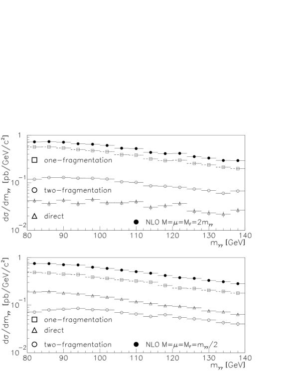
3.2 Predictions for LHC
We now discuss some results computed with the kinematic cuts from the CMS and ATLAS proposals [40], namely GeV, GeV, , with GeV GeV, and using the MRST2 set of parton distribution functions [37] and the fragmentation functions of [10].
3.2.1 Scale ambiguities
We first consider the invariant mass distribution of diphotons, in absence of
isolation cuts, cf. Fig. 6 in order to illustrate the
strong dependence of the splitting into the three contributions, “direct”,
“one-” and “two fragmentation”, on the scale chosen, as we warned in 2.1.
In both choices of scales displayed the “one fragmentation” contribution
dominates, but the hierarchy between “direct” and ”two fragmentation”
contributions is reversed from one choice to the other. With the choice of scales , the
“one fragmentation” is more than twice larger than the “direct” one, and
the “two fragmentation” is the smallest. On the other hand, with the other
choice , the “one fragmentation”
contribution is three to five times larger than the “two fragmentation”
component, and more than one order of magnitude above the “direct”
one. On the other hand the total contribution seems rather stable.
Yet the arbitrariness in the choices of the various scales still induces theoretical
uncertainties in NLO calculations. In the following we actually do not perform
a complete investigation of all three scale ambiguities independently with
search for an optimal region of minimal sensitivity. At the present stage, we
limit the study to an estimation of the pattern and magnitude of their effect
on our results. We show how the scale ambiguities affect our prediction for the
invariant mass distribution. We consider both the case without isolation (Fig.
7) and the isolated case with GeV
inside (Fig. 8). For the present purpose,
the virtue of the actual values of the isolation parameters used here is to
strongly suppress the fragmentation contributions hence the associated
dependence. We compare four different choices of scales: two choices
along the first diagonal and
; and two anti diagonal choices,
and
. We do not
perform a separate study of fragmentation scale dependence. Yet the latter can
be indirectly estimated by comparing the results of the isolated case, where
the fragmentation components, thereby the corresponding fragmentation scale
dependence, are strongly suppressed, with the situation in the non isolated
case, where especially the “one fragmentation” contribution is quite large,
and the “two fragmentation” not negligible, so that the issue of fragmentation
scale dependence matters.
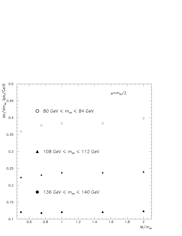
When scales are varied between and along the first diagonal , the NLO results for the
invariant mass distribution appear surprisingly stable, since they change by
about 5% only. Alternatively, anti-diagonal variations of and in the same interval about the central value lead
to a variation still rather large (up to 20 % cf. Fig.
7 and Fig. 8). This is because variations
with respect to and are separately monotonous but act in opposite ways.
When is increased, hence the NLO corrections
decrease141414 In processes for which the lowest order is proportional to
some power , an explicit dependence appears in
the next-to-leading order coefficient function, which partially compensates the
(large) dependence in weighting the lowest order.
Unlike this, in the “two direct” component which dominates the cross section
when a drastic isolation is required, the lowest order involves no
. This leads to a rather small dependence, since the latter
starts only at NLO. On the other hand, the dependence occurs only
through the monotonous decrease of the weighting the
first higher order correction: there is no partial cancellation of
dependence. Such cancellation would start only at ,
i.e. at NNLO. The mechanism is more complicated in presence of fragmentation
components, and the situation becomes mixed up between all components when the
severity of isolation is reduced.. On the other hand the relevant values of
momentum fraction of incoming partons are small, to
so that the gluon and sea quark distribution functions increase when
is increased. In the isolated case, this leads to a monotonous increase of
the “direct” component, over a large band of the invariant mass range
considered, as is increased, cf. Fig. 9, which is induced
in particular by the monotonous increase of the box contribution. Scale
changes with respect to and turn out to nearly cancel against each
other along the first diagonal but add up in the other case. Actually, the
stability along the first diagonal is accidental.
In conclusion, the , dependences are thus not completely under control
yet at NLO in the kinematic range considered. On the opposite, the account
for the NLO corrections to the fragmentation components provides some
stability with respect to variations about orthodox choices of the
fragmentation scale.
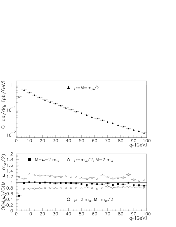
The issue of dependence of less inclusive observables, such as the tails
of the or distributions are the same for the
invariant mass distribution. This is because the tails of these distributions
is purely given by the NLO corrections and dominated by the corrections of the “two direct” component. On the other hand,
the dependence is a bit larger, so is the combined uncertainty on the
theoretical results for these distributions, cf. Fig. 10 and
Fig. 11.
3.2.2 Effect of isolation
We now consider the effect of isolation on the various contributions. As
expected, isolation reduces the diphoton production rate, with respect to the
inclusive case, cf. Fig. 12. More precisely, severe isolation requirements like
GeV inside a cone suppress the “one
fragmentation” component, which dominates the inclusive rate, by a factor 20 to
50, and kill the “two fragmentation” contribution completely.
However this net result hides a rather intricate mechanism, cf. Fig.
13 vs. Fig. 6, by which the “two direct” contribution turns
out to be increased! Surprising as it may seem at first sight, this effect has
the following origin. Higher order corrections to the “two direct” component
involve in particular the two subprocesses and (where is a quark or an
antiquark). The first one yields a positive contribution. On the other hand,
the collinear safe part of the second one yields a contribution which is
negative, and larger in absolute value than the previous one in the inclusive
case, as was already seen in [7]. Isolation turns out to suppress more
the higher order corrections from the second mechanism than from the first one,
so that the NLO isolated “two direct” contribution is larger than the
inclusive one. Yet, the “fragmentation” contributions are suppressed more than
the “two direct” one is increased, so that the sum of all contributions is
indeed decreased, with respect to the inclusive case. Once again, one has to
remember that the splitting into the three mechanisms depend, not only on the
factorization scale, but more generally on the factorization scheme. This
arbitrariness generates such counterintuitive offsprings; in a final state
factorization scheme different than the scheme, the various
components, especially the “two direct” one, may be separately affected by
isolation cuts in a different way. This once more illustrates the danger of
playing with these unphysical quantities separately.
A more detailed analysis of the dependence of NLO estimations of various
observables on the isolation cut parameters, especially on will
be given in a forthcoming publication. We will also come back to this issue,
regarding infrared sensitivity, in 4.3.
4 Infrared sensitive observables of photon pairs and soft gluon divergences.
Being based on a fixed, finite order calculation, our computer code is not suited for the study of observables controlled by multiple soft gluon emission, and has to be improved in this direction. Among these infrared sensitive observables, one may distinguish the following examples, most of which would require an improved account of soft gluon effects.
4.1 Infrared sensitivity near the elastic boundary
4.1.1 The transverse momentum distribution of photon pairs near
Both in the inclusive and isolated cases, this distribution is an infrared
sensitive observable, controlled by the multiple emission of soft and
collinear gluons. This well known phenomenon has been extensively studied for
the corresponding observable in the Drell-Yan process [41]. A loss
of balance between the contribution of real emission, strongly suppressed near
this exclusive phase space boundary, and the corresponding virtual
contribution, results in large Sudakov-type logarithms of
( being the invariant mass and and the transverse momentum of the
photon pair - the heavy vector boson in the Drell-Yan case) at every order in
perturbation. In order to make sensible predictions in this regime, these
Sudakov-type logarithms have to be resummed to all orders.
The treatment of the “two direct” and box contributions is similar to the well-known Drell-Yan process, and has been carried out recently by [42] at next-to-leading logarithmic accuracy in the framework tailored by Collins, Soper and Sterman [43]. On the other hand, the fragmentation contributions do not diverge order by order when . Indeed, in the “one fragmentation” case,
| (2) | |||||
| (3) |
the NLO contribution to the hard subprocess (2) yields a double logarithm of the form
| (4) |
when .
However the extra convolution associated with the fragmentation
(3) involves an integration over the fragmentation variable
which
smears out this integrable singularity. The “two fragmentation”
contribution involves two such convolutions, hence one more smearing.
4.1.2 The distribution of photon-photon azimuthal angle near
This distribution is another interesting infrared sensitive observable, measured by several experiments both at fixed target and collider energies [2, 5, 6], though less discussed in the literature from the theoretical side. The regime includes back-to-back photons, a set of configurations which lie at the elastic boundary of the phase space. This case differs from the previous one for two reasons. Firstly, not only the “two direct” contribution diverges order by order when , but also both “one-” and “two fragmentation” contributions diverge as well, as can be inferred from Fig. 5. Indeed, consider the example of the “one fragmentation case”, cf. equations 2 and 3. Selecting emphasizes the configurations with , so that all the emitted partons besides parton 3 have to be collinear to either of the incoming or outgoing particles, and/or soft, which yields double logarithms
| (5) |
associated with each of the hard partons - plus single
logarithms as well. For the observable
near
, the integral involved in the convolution of the
hard subprocess with the fragmentation functions does not smear these
logarithmic divergences, since the fragmentation variable
is
decoupled from the azimuthal variable
which is equal to ,
and parton being collinear. A similar observation holds for the “two
fragmentation” component. Moreover, in both fragmentation cases,
soft gluons may couple to both initial and final state hard emitters. The
resulting color structure of
the emitters is more involved than in the “two direct” case, and especially
more complicated in the “two fragmentation” case as shown in some recent works
[44]. This would make any resummation
quite intricate beyond leading logarithms.
Let us notice that both fragmentation components make diverge also when . The increase of the fragmentation contributions in the lower range is the trace of this divergence, cf. Fig. 5.
4.2 An infrared divergence inside the physical region.
In the case of photons isolated with the standard fixed cone size criterion of eqn. (1), a new problem appears in the distribution. This problem does not concern the region ; still it has to do with infrared and collinear divergences. This can be seen on Fig. 14, which shows the observable vs. for isolated photon pairs, computed at NLO accuracy. The computed distribution turns out to diverge when from below. Notice that the critical point is located inside the physical region. The phenomenon is similar to the one discovered in [25] in the production of isolated photons in annihilation, and whose physical explanation has been given in [30] following the general framework of [45]. It is a straightforward exercise to see that the lowest order “one fragmentation” contribution has a stepwise behaviour, as noticed in [9]. Indeed, at this order, the two photons are back-to-back. being the transverse hadronic energy deposited in the cone about the photon from fragmentation, the conservation of transverse momentum implies at this order that . The corresponding contribution to the differential cross section thus takes the schematic form:
| (6) |
According to the general analysis of [45], the NLO correction to has a double logarithmic divergence at the critical point 151515In practice, the spectrum is sampled into bins of finite size, and the distribution represented on Fig. 14 is averaged on each bin. Since the logarithmic singularity is integrable, no divergence is actually produced. However when the bin size is shrunk, the double logarithmic branch appears again.. The details of this infrared structure are very sensitive to the kinematic constraints and the observable considered. In the case at hand, at NLO, gets a double logarithm below the critical point, which is produced by the convolution of the lowest order stepwise term above, with the probability distribution for emitting a soft and collinear gluon:
| (7) | |||||
where is a color factor, or according to whether the
soft collinear gluon emitter is a quark (antiquark) or a gluon.
More generally, at each order in , up to two powers of such
logarithms will appear, making any fixed order calculation diverge at
, so that the spectrum computed by any fixed order
calculation is unreliable in the vicinity of this critical value. An all order
resummation has to be carried out if possible in order to restore
any predictability. A correlated step appears also in the “two direct”
contribution at NLO, in the bin about . A detailed
study of these infrared divergences will be presented in a future article.
No such divergence appears in the distribution of
photon pairs presented in [9]. The non
appearance of the double logarithmic divergence there comes from the
fact that the latter pops out only at NLO, while
the authors of [9] compute the “one
fragmentation” component at lowest order.
Furthermore, the stepwise lowest order “one fragmentation” contribution
to the distribution is replaced in
[9] by the result of the Monte Carlo simulation
of this component using PYTHIA [20]. A quantitative comparison
is thus difficult to perform161616Such a comparison involves two issues.
The first aspect concerns the infrared sensitivity below the critical
point. When the scale of in the Sudakov
factor of the fragmenting quark is chosen to be the transverse momentum
of the emitted gluon with respect to the emitter, the parton shower not
only reproduces the fragmentation function of a parton into a photon to the collinear leading logarithmic approximation, but
it also provides an effective resummation of soft gluons effects to
infrared and collinear leading logarithmic accuracy. (This would not be true if,
instead, the scale of in the Sudakov factor were the
virtuality of the emitter). This ensures that the distribution does not
diverge from below at the critical point, but rather tends to a finite
limit.
The second issue concerns the shape of the tail of this contribution above the
critical point. Indeed, energy-momentum conservation at each branching makes
the parton shower generate also contributions in the region
, which is forbidden at lowest order. These
contributions would be classified in a beyond leading order calculation as
higher order corrections. Unlike in a fixed order calculation however, they
provide only a partial account of such corrections, but to arbitrary high
order. The accuracy of these terms is thus uneasy to characterize, and a
quantitative comparison between PYTHIA and any fixed order calculation is
difficult to perform..
It can be noticed that the divergence at is not visible on Fig. 4. This is because in this case, the critical point in the spectrum where the theoretical calculation diverges is too close to the other singular point , given the binning used. The two singularities contribute with opposite signs in these bins and a numerical compensation occurs, resulting in no sizeable effect. Yet the problem is only camouflaged. A similar smearing appears also at LHC energies for a stringent isolation cut, cf. Fig. 10.
4.3 Reliability of NLO calculations with stringent isolation cuts
Let us add one more comment concerning NLO partonic predictions with very
stringent isolation cuts. In such calculations, the isolation cuts act on the
products of the hard subprocess only. On the other hand, in an actual LHC event, a
cut as severe as GeV inside a cone or
will be nearly saturated by underlying events and pile up.
This means that such an isolation cut actually allows almost no transverse energy deposition from the actual hadronic products of the hard process itself. This may be most suitable experimentally, and one may think about simulating such an effect safely in an NLO partonic calculation by using an effective transverse energy cut much more severe than the one experimentally used. However, requiring that no transverse energy be deposited in a cone of fixed size about a photon is not infrared safe, i.e. it would yield a divergent result order by order in perturbation theory. This implies that NLO partonic calculations implemented with finite but very stringent isolation cuts in a cone of fixed finite size would lead to unreliable results, plagued by infrared instabilities involving large logarithms of . What is more, these infrared nasties would not be located at some isolated point in the diphoton spectrum (like some elastic boundary or some critical point, as in the previous subsection), but instead they would extend over its totality, even for observables such as the invariant mass distribution. The issue of an all order summation of these logarithms of would have to be investigated in this case.
5 Conclusions and perspectives
We presented an analysis of photon pair production with high invariant mass in
hadronic collisions, based on a perturbative QCD calculation of full NLO
accuracy. The latter is implemented in the form of a Monte Carlo computer
programme of partonic event generator type, DIPHOX. The postdictions of
this study are in reasonable agreement with both WA70 fixed target, and
preliminary D0 collider data, in the kinematical range where the NLO
approximation is safe, namely away from the elastic boundary of phase space.
Yet more will be learnt from the final analysis of the Tevatron data, and even
more so after the Tevatron run II in the perspective of the LHC. It will then
be worthwhile to perform a more complete phenomenological study.
This notwithstanding, there remains room for improvements. A first improvement
will be to take into account multiple soft gluon effects
in order to calculate infrared sensitive observables correctly. Another
improvement will concern a more accurate account of contributions beyond NLO,
associated namely with the gluon-gluon initiated subprocess. Among those are
the NNLO corrections, and even the two loop, so-called double box correction to
, which may be quantitatively important at LHC
for the background to Higgs search.
A better understanding of the effects of isolation, and their interplays with
infrared problems is also required. This concerns the distribution near
the critical point induced by isolation even
when is not small; this concerns also the status of partonic
predictions when is chosen very small. Alternatively it would be
interesting to explore the properties of different isolation criteria, such
as, for example, the one invented recently by Frixione [22].
Concerning these last two items, approaches relying on beyond leading order
partonic level calculations, and full event generators like PYTHIA or HERWIG
will be
complementary.
Acknowledgments
We acknowledge discussions with J. Womersley and T.O. Mentes on the D0 data, J. Owens on theory vs. data comparisons, and C. Balazs about the theoretical ingredients inside the RESBOS code. We thank F. Gianotti, P. Petroff, E. Richter-Was and V. Tisserand for discussions concerning the Atlas Proposal. This work was supported in part by the EU Fourth Training Programme “Training and Mobility of Researchers”, Network “Quantum Chromodynamics and the Deep Structure of Elementary Particles”, contract FMRX-CT98-0194 (DG 12 - MIHT).
Appendix A Technical details on the two photon production
In this appendix, we give some details on the method used to deal with infrared and soft divergences. For a complete presentation, we refer to [15]. The most complicated kinematics happens in the two fragmentation mechanism. Only the two fragmentation contribution will be treated in this appendix, the kinematics of the other cases can be simply deduced replacing the fragmentation function by a Dirac distribution:
At the hadronic level, the reaction is considered with:
where
The cross section of the preceding reaction is the sum of the following parts.
-
-
The part I (cf. sect. 2.2.1) contains the infrared, the initial state, and a part of the final state collinear singularities. Once these divergences have been subtracted, i.e. cancelled against virtual divergences or absorbed into the bare parton distribution (for the initial state collinear singularities) or the bare fragmentation functions(for the final state collinear singularities), this part generates three types of finite terms.
-
(i)
The first type, of infrared origin, has the same kinematics as the lowest order (LO) terms and is given in A.4 Pseudo cross section for the infrared and virtual parts.
-
(ii)
The second type, of initial state collinear origin, has an extra integration over the center of mass energy of the hard scattering, as compared to LO kinematics. For this reason, it is called quasi . It is given in A.2 Pseudo cross sections for the initial state collinear parts.
-
(iii)
There is also a third type, of final state collinear origin, which involves also an extra integration as compared to LO kinematics.
-
(i)
-
-
The parts II a and II b contain the rest of the final state collinear singularities. Once these divergences have been absorbed into the bare fragmentation functions, the remaining finite terms involve an extra integration over the relative momentum of the collinear partons, as compared to LO kinematics. These terms are combined with those of the so called third type (iii) above, cf. equations (A.3) and (A.3). The resulting contributions are called quasi as well. They are given in A.3 Pseudo cross sections for the final state collinear parts.
-
-
The part II c has no divergences. It is given in A.1 Cross section for real emission.
A.1 Cross section for real emission
The cross section is parametrized in the following way:
| (A.1) | |||||
where
| (A.4) | |||||
| (A.5) |
The transverse momenta (resp. ) are the transverse momenta of the fragmenting partons. They are related to the photon variables by (resp. ). The integration range for the pair of variables (resp. ), is the kinematically allowed range minus a cone in rapidity azimuthal angle (resp. ) along the (resp. ) direction whose size is . The overall factor reads:
and the are given by:
The matrix element squared 171717An overall factor of the matrix element squared containing the average on spins and colors of the initial state and the coupling constant has been put into the coefficient , taken from the first reference of [7] and [46], has been split into two parts:
The first part contains final state collinear singularities arising when // and the second part contains final state collinear singularities arising when // . More precisely, the matrix element squared can be written as a weighted sum of eikonal factors plus a term free of infrared or collinear singularities:
| (A.6) |
where
Using:
| (A.7) |
we get:
with
In order that the infrared divergences cancel, and the collinear singularities factorize out, the coefficients have to fulfill:
In particular, the cancellation of infrared divergences is insured by:
The functions will be given in equation (A.13).
In equation (A.1), the integration domain for the rapidities and the transverse momenta of the two photons is in general limited by experiments. The integration over is constrained by:
A.2 Pseudo cross sections for the initial state collinear parts
The finite part associated to the collinear divergence // is given by:
| (A.8) | |||||
where the variables (resp. ) are defined by:
and stands for or .
The finite part associated to the collinear divergence // is given by:
| (A.9) | |||||
with
A.3 Pseudo cross section for the final state collinear parts
These parts contain the collinear singularities which have been absorbed into the bare fragmentation functions.
The finite part associated to the collinear divergence // is given by:
whereas the finite part associated to the collinear divergence // is given by:
A.4 Pseudo cross section for the infrared and virtual parts
This pseudo cross section is given by:
| (A.12) | |||||
with . The terms are defined in equations (A.22) and (A.23). In the equation (A.12), and the function is given by:
The function is the finite part of the virtual term and the variables , and are the Mandelstam variables of the processes:
where the 4-vectors are the infrared limits of the 4-vectors .
A.5 Altarelli-Parisi Kernels
We will give in this appendix the expressions of the functions and . These functions are defined by:
| (A.13) | |||||
where (resp. ) are the Altarelli-Parisi Kernels in four (resp. ) dimensions. So the expressions for the functions , and are given by:
| (A.14) | |||||
| (A.15) | |||||
| (A.16) | |||||
| (A.17) |
where is the number of colors, and . The extra part needed to get the functions in dimensions () is given by:
| (A.18) | |||||
| (A.19) | |||||
| (A.20) | |||||
| (A.21) |
The coefficients read:
| (A.22) | |||||
| (A.23) |
The function and define the factorisation scheme for respectively initial state and final state collinear singularities. In the scheme, we have:
| (A.24) | |||
| (A.25) |
Appendix B Cancellation of the and dependences
In this appendix, we give further details on the cancellation of the
and dependences in observables calculated according to the method used
in this article.
In the conical parts II a and II b, the -dimensional integration over particle 5 in , , reads schematically:
| (B.1) | |||||
The term generating the final state collinear pole (//) has been explicitly written, and the remaining quantity is a regular function. In the parts II a and II b, the same subtraction method as in [15] is used, and the following contribution is added and subtracted:
| (B.2) |
In the cylindrical part I, the finite terms produced by the integration over
particle 5 are approximated: all the terms depending logarithmically on
are kept, whereas terms proportional to powers of
are neglected. Notice that this differs from the subtraction method implemented
in the cylinder in [15], which kept the exact dependence.
In summary, the present method is an admixture of the phase space slicing and
subtraction methods, at variance with what has been done in [15]. It
ensures the exact cancellation of the unphysical parameter dependence
between part II c and parts II a, II b whereas only an approximated
cancellation of the unphysical parameter dependence between parts II
c, II a and II b and part I occurs.
We checked carefully that the dependences on the unphysical parameters drop out. This point is illustrated by the dependence (at fixed ) and the dependence (at fixed GeV), of the higher order (HO) part of integrated cross section (the lowest order (LO) part being independent of these parameters)
shown on Figs. 15 and 16. We display
separately the and initiated contributions to the “direct”
on Fig. 15, and the “one-” and “two fragmentation”
mechanisms, on Fig. 16. To be definite, the integration bounds
are taken to be GeV, GeV, the cuts ,
GeV, are applied, and the MRST2 set of
parton distribution functions with the scale choice are used; let us emphasize however that the pattern obtained does
not depend on these details.
The quantity does not depend on and, in principle, it becomes independent of at small enough . To show these features more clearly, the observable displayed is the ratio defined as follows:
| (B.3) |
The integrated cross section is normalized to be asymptotically 1 in order to show the size of the relative error bars. However taking the denominator equal to the calculated for the smallest value of may be numerically unsuitable. Indeed, when becomes smaller and smaller, numerical cancellations between larger and larger contributions occur and the error bars coming from the Monte Carlo integration become larger and larger. These numerical fluctuations affect the behavior in the limit . In order to bypass these technical complications, is taken to be the averaged value of those of the integrated cross sections which are consistent with each other within the error bars. For instance, for the dependence of the “direct” contribution, the average is taken over the values corresponding to the three smallest because the fourth one is not consistent with the others in the error bars. In addition, in the case of the direct contribution, the two partonic reactions and have been split because, for the above choices of scales, the two integrated contributions are large and of opposite signs. As expected, does not depend on and approaches 1 as . Let us notice that one can wonder whether large relative fluctuations do not appear again when the two contributions of the “direct” are added. Indeed, the relative fluctuations of the HO terms are larger for the sum than for each parts, but these HO terms are small compared to the LO part () hence the “physical” cross section (LO+HO) is sufficiently stable. When the parameter is chosen small enough with respect to and , the neglected terms power behaved in can be safely dropped out. In practice, we observe that values of the order of half a percent of the minimum and , i.e. GeV, fulfill these requirements. Before embarking in a long phenomenological study, the user of the DIPHOX code is advised to check whether the value of the parameter to be used is small enough to neglect safely the power corrections of .
References
- [1] WA70 Collaboration, E. Bonvin et al., Z. Phys. C41 (1989) 591.
- [2] WA70 Collaboration, E. Bonvin et al., Phys. Lett. 236B (1990) 523.
- [3] Private communication from M. Begel (E706 collaboration).
- [4] UA2 Collaboration. J. Alitti et al., Phys. Lett. 288B (1992) 386.
- [5] CDF Collaboration, F. Abe et al., Phys. Rev. Lett. 70 (1993) 2232.
-
[6]
Wei Chen, PhD Thesis (Univ. New-York at Stony Brook), Dec. 1997, unpublished;
D0 Collaboration (P. Hanlet for the collaboration), Nucl. Phys. Proc. Suppl. 64 (1998) 78.
All the numbers used in this article are taken from tables in Wei Chen PhD Thesis. -
[7]
P. Aurenche, R. Baier, A. Douiri, M. Fontannaz and D. Schiff,
Z. Phys. C29 (1985) 459;
P. Aurenche, M. Bonesini, L. Camilleri, M. Fontannaz and M. Werlen, Proceedings of LHC Aachen Workshop CERN-90-10 G. Jarlskog and D. Rein eds., vol. II, p. 83. -
[8]
B. Bailey, J. Ohnemus and J.F. Owens,
Phys. Rev. D46 (1992) 2018;
B. Bailey and J.F. Owens, Phys. Rev. D47 (1993) 2735;
B. Bailey and D. Graudenz, Phys. Rev. D49 (1994) 1486. -
[9]
C. Balazs, E.L. Berger, S. Mrenna and C.P. Yuan,
Phys. Rev. D57 (1998) 6934;
C. Balazs and C.P. Yuan, Phys. Rev. D59 (1999) 114007. - [10] L. Bourhis, M. Fontannaz and J.Ph. Guillet, Eur. Phys. J. C2 (1998) 529.
- [11] A. Djouadi, D. Graudenz, M. Spira and P. Zerwas, Nucl. Phys. B453 (1995) 17.
- [12] V. Del Duca, W.B. Kilgore and F. Maltoni, hep-ph/9910253.
-
[13]
D. de Florian and Z. Kunszt, Phys. Lett. 460B (1999) 184;
C. Balazs, P. Nadolsky, C. Schmidt and C.P. Yuan, hep-ph/9905551. -
[14]
V.A. Smirnov, Phys. Lett. 460B (1999) 397;
J.B. Tausk, hep-ph/9909506. - [15] P. Chiappetta, R. Fergani and J.-Ph Guillet, Z. Phys. C69 (1996) 443.
-
[16]
M.A. Furman Nucl. Phys. B197 (1982) 413;
W.T. Giele and E.W.N. Glover, Phys. Rev. D46 (1992) 1980;
W.T. Giele, E.W.N. Glover and D. Kosower, Nucl. Phys. B403 (1993) 633. -
[17]
R.K. Ellis, D.A. Ross and A.E. Terrano, Nucl. Phys. B187 (1981) 421;
S. Frixione, Z. Kunszt and A. Signer, Nucl. Phys. B467 (1996) 399;
S. Catani and M.H. Seymour, Nucl. Phys. B485 (1997) 291. - [18] S. Kawabata, Comp. Phys. Comm. 88 (1995) 309.
-
[19]
R. Brun, O. Couet, G.E. Vandoni and P. Zabarini,
Comp. Phys. Comm 57 (1989) 432;
PAW, Physics Analysis Workstation, CERN Program Library Q121
(http://wwwinfo.cern.ch/asd/paw/index.html). -
[20]
H.-U. Bengtsson and T. Sjöstrand, Comp. Phys. Comm. 46 (1987) 43;
T. Sjöstrand, Comp. Phys. Comm. 82 (1994) 74;
T. Sjöstrand, LU TP 95-20, hep-ph/9508391. -
[21]
G. Marchesini and B.R. Webber, Nucl. Phys. B 310 (1988) 461;
G. Marchesini, B.R. Webber, G. Abbiendi, I.G. Knowles, M.H. Seymour and L. Stanco, hep-ph/9607393. - [22] S. Frixione, Phys. Lett. 429B (1998) 369.
- [23] H. Baer, J. Ohnemus and J.F. Owens, Phys. Rev. D42 (1990) 61.
- [24] P. Aurenche, R. Baier and M. Fontannaz, Phys. Rev. D42 (1990) 1440.
- [25] E.L. Berger and J. Qiu, Phys. Rev. D44 (1991) 2002.
- [26] L.E. Gordon and W. Vogelsang, Phys. Rev. D50 (1994) 1901.
- [27] S. Catani, M. Fontannaz and E. Pilon, work in preparation.
- [28] Z. Kunszt and Z. Troscanyi, Nucl. Phys. B394 (1993) 139.
- [29] E.L. Berger, X.F. Guo and J.W. Qiu, Phys. Rev D54 (1996) 5470.
- [30] S. Catani, M. Fontannaz and E. Pilon, Phys. Rev. D58 (1198) 094025.
- [31] E.W.N. Glover and A.G. Morgan, Z. Phys. C62 (1994) 311.
- [32] P. Aurenche, R. Baier, M. Fontannaz, J. Owens and M. Werlen, Phys. Rev. D39 (1989) 3275.
- [33] P. Aurenche, R. Baier, M. Fontannaz, M.N. Kienzle-Foccacci and M. Werlen, Phys. Lett. 233B (1989) 517.
- [34] P.J. Sutton, A.D. Martin, R.G. Roberts and W.J. Stirling, Phys. Rev. D45 (1992) 2349.
- [35] M. Glück, E. Reya and A. Vogt, Z. Phys. C53 (1992) 651.
- [36] B. Abbott et al., Phys. Rev. D58 (1998) 092003
- [37] A.D. Martin, R.G. Roberts, W.J. Stirling and R.S. Thorne, hep-ph/9907231.
- [38] J. Womersley, private communication.
- [39] J.F. Owens, private discussion.
-
[40]
CMS technical proposal CERN/LHCC 94-38 (p 179);
ATLAS technical proposal CERN/LHCC 94-43;
V. Tisserand for the ATLAS collaboration, in Proc. 6th Int. Conf. on Calorimetry in High Energy Physics (ICCHEP 96), ed. by A. Antonelli, S. Bianco, A. Calcaterra, F.L. Fabbri, (Frascati physics series; 6) p 475. -
[41]
Y. Dokshitzer, D. Dyakonov and S. Troyan, Phys. Rep. 58 (1980) 269;
A. Basseto, M. Ciafaloni and G. Marchesini, Phys. Rep. 100 (1983) 201 and references therein;
see also [43]. - [42] C. Balazs, private communication.
-
[43]
J. Collins and D. Soper, Nucl. Phys. B193 (1981) 381;
J. Collins and D. Soper, Nucl. Phys. B197 (1982) 446;
J. Collins, D. Soper and G. Sterman, Nucl. Phys. B250 (1985) 199. -
[44]
R. Bonciani, S. Catani, M. Mangano and P. Nason, Nucl. Phys. B529 (1998) 424;
N. Kidonakis, G. Oderda and G. Sterman, Nucl. Phys. B531 (1998) 365. - [45] S. Catani and B. Webber, JHEP 9710:005 (1997).
- [46] R. K. Ellis and J. C. Sexton, Nucl. Phys. B269 (1986) 445.