Quark-Antiquark Bound States in the
Relativistic Spectator Formalism

Abstract

The quark-antiquark bound states are discussed using the relativistic spectator (Gross) equations. A relativistic covariant framework for analyzing confined bound states is developed. The relativistic linear potential developed in an earlier work is proven to give vanishing meson$\rightarrow$ $q+\bar{q}$ decay amplitudes, as required by confinement. The regularization of the singularities in the linear potential that are associated with nonzero energy transfers (i.e. $q^{2}=0,q^{\mu}\neq 0$) is improved. Quark mass functions that build chiral symmetry into the theory and explain the connection between the current quark and constituent quark masses are introduced. The formalism is applied to the description of pions and kaons with reasonable results.

I Introduction

Description of simple hadrons in terms of quark-gluon degrees of freedom has long been an active area in physics. With the advent of Jefferson Laboratory, which operates at intermediate energies and therefore probes the structure of hadrons, there are new opportunities to test simple theoretical descriptions of quark interactions. The first natural step in this direction is a thorough understanding of how to treat the relativistic quark-anti quark bound state problem. In this context, NJL inspired models have gained popularity in recent years[1, 2]. The common goal of these works is to bridge the gap between nonrelativistic quark models and more rigorous approaches, such as lattice gauge theory or Feynman-Schwinger calculations. While the Euclidean metric based calculations are increasingly popular, their applicability, because of the extrapolations involved, is only limited to light bound states such as the pion and kaon. Therefore, it is important to develop Minkowski metric based models which can be used over a wider scale of energies. One such work using the spectator formalism was developed in Ref. [1]. In those works a relativistic generalization of the linear potential was developed and the pion was shown to be massless in the chiral limit. However, the calculations involved some approximations and related conceptual problems. In this work we improve and simplify the model presented in those works and address in detail some of the conceptual issues related to confinement.

If a quark-antiquark pair (referred to collectively as “quarks”) is confined to a meson bound state with mass $\mu$, then the bound state can not decay into two free quarks, even if the sum of the quark masses is less than the bound state mass. This trivial statement can be realized by two possible mechanisms: either (a) the quark propagators are free of timelike mass poles,[2] or (b) the vertex function of the bound state vanishes when both quarks are on-shell. In this work we prove that the Gross equation supports the second mechanism of confinement. The first mechanism, which is commonly used in Euclidean metric based calculations, is a stronger constraint since it forbids any free quark states. On the other hand, the Gross equation allows one of the two quarks in a meson to be on-shell, but insures that the matrix element which couples the bound state to two free quarks vanishes. The spectator formalism facilitates the use of the Minkowski metric, and the confinement mechanism of this approach has a closer resemblance to nonrelativistic models.

The organization of the paper is as follows: In Sec. II we review the formalism for nonrelativistic confinement in momentum space. In Sec. III we outline the general philosophy of the spectator approach to the treatment of confined systems, examine the implications of confinement for the scattering amplitude, and prove that the relativistic linear potential used in earlier works automatically insures that $\mu\rightarrow q+\bar{q}$ vanishes at the momentum where decay of the state into two physical quarks would otherwise be kinematically possible. The treatment is first presented for scalar particles, and then generalized to fermions. In Sec. IV we construct quark mass functions that have the correct chiral limit and preserve asymptotic freedom. Our numerical results for pseudoscalar bound states are presented in Sec. V, and some conclusions are given in Sec. VI.

II Nonrelativistic confinement in momentum space

We start by reviewing the discussion of confinement within the context of the nonrelativistic Schrödinger equation given in Ref. [1]. We will denote potentials in coordinate space by $\tilde{V}$ and in momentum space by $V$. The nonrelativistic linear potential is

$$\tilde{V}(r)=\sigma r\,.$$ (1)

This potential can be constructed from familiar Yukawa-like potentials in two different ways:

$$\tilde{V}(r)=\lim_{\epsilon\to 0}\cases{\tilde{V}_{S}(r)\equiv\sigma re^{-\epsilon r}&\rm{(a)}\cr\tilde{V}_{L}(r)\equiv-{\displaystyle{\frac{\sigma}{\epsilon}}}\left(e^{-\epsilon r}-1\right)=\tilde{V}_{A}(r)+{\displaystyle\frac{\sigma}{\epsilon}}\,.\qquad\qquad&\rm{(b)}}$$ (2)

These various potentials are shown in Fig. 1 for the illustrative case of $\epsilon=0.1$ and $\sigma=0.2$.

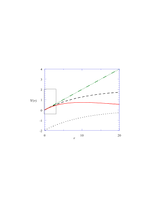
FIG. 1.: The linear potential in coordinate space for $\epsilon=0.1$ and $\sigma=0.2$. The solid line is $\tilde{V}_{S}(r)$, the dashed line is $\tilde{V}_{L}(r)$, the dotted line is $\tilde{V}_{A}(r)$, and the dot-dashed line is $\tilde{V}(r)$. For “small” $r<1/\epsilon$ (the region inside the small box) $\tilde{V}_{L}(r)$ and $\tilde{V}_{S}(r)$ are both approximately equal to $\sigma r$.

Note that the two potentials $\tilde{V}_{S}(r)$ and $\tilde{V}_{L}(r)$ both approximate the linear potential $\tilde{V}(r)$ when $r<<1/\epsilon$, but that these two approximate potentials behave very differently at large $r$. The potential $\tilde{V}_{S}(r)\to 0$ at large $r$, so that, strictly speaking, it does not confine particles at all. This potential always permits scattering, although when $\epsilon$ is small the scattering is strongly resonant, and the wave function is significant at small $r$ only for energies near one of the allowed resonances. The width of these resonance states becomes narrower, and their wave function approaches that of a bound state, as $\epsilon\to 0$. In contrast, the potential $\tilde{V}_{L}(r)\to 1/\epsilon$ as $r\to\infty$ and therefore binds particles with energies $E<1/\epsilon$. As $\epsilon\to 0$ this potential does not permit scattering; it has a spectrum of bound states only.

Yet for sufficiently small $\epsilon$, it should be possible to move freely from one of these potentials to the other, and the results obtained with either form should be equivalent. We will return to this later in this section. Now we follow Ref. [1] and work with $\tilde{V_{L}}$ given in Eq. (2b).

The momentum space form of this potential can be written

$$V_{L}({\bf q})= \lim_{\epsilon\rightarrow 0}\;\left[V_{A}({\bf q})-\delta^{3}({q})\int d^{3}q^{\prime}\,V_{A}({\bf q}^{\prime})\right]\,,$$ (3)

where

$$V_{A}({\bf q})=-\frac{8\pi\sigma}{({\bf q}^{2}+\epsilon^{2})^{2}}\,,$$ (4)

Note that the second term (the “subtraction term”) insures that

$$\int d^{3}q\;V_{L}({\bf q})=0\,,$$ (5)

which is the momentum space form of the statement that $\tilde{V}(r=0)=0$. The Fourier transform of $V_{A}$ is, for finite $\epsilon$,

$$\tilde{V}_{A}({\bf r}) = \int\frac{d^{3}q}{(2\pi)^{3}}\,e^{-iq\cdot r}\,V_{A}({\bf q})$$ (6)

$$= -\sigma\frac{e^{-\epsilon r}}{\epsilon}\ \ \simeq\ \ \lim_{\epsilon\rightarrow 0}\sigma\left(r-\frac{1}{\epsilon}\right)\,,$$ (7)

and the subtraction term cancels the singular $1/\epsilon$ term insuring that the linear part of the potential has the correct behavior in the limit as $\epsilon\to 0$ and that it vanishes at the origin ($r=0$). Now, adding a constant potential $V_{C}$

$$V_{C}(r)= -C$$ (8)

$$V_{C}({\bf q})= -(2\pi)^{3}\delta^{3}({q})C\,,$$ (9)

to the linear potential (3), and inserting the total potential into the momentum space Schrödinger equation gives

$$\left[\frac{{\bf p}^{2}}{2m_{R}}-E\right]\Psi({\bf p},p_{0})=-\int\frac{d^{3}k}{(2\pi)^{3}}V_{A}({\bf p}-{\bf k})\,\left[\Psi({\bf k},p_{0})-\Psi({\bf p},p_{0})\right]+C\,\Psi({\bf p},p_{0})\,,$$ (10)

where $m_{R}$ is the reduced mass, $E$ is the binding energy, and $p_{0}$ is an eigenvalue given by

$$p_{0}^{2}=2m_{R}E\,.$$ (11)

The constant potential is used to adjust the energy scale.

While Eq. (10) was derived for the linear potential with the specific choice of $V_{A}$ given in Eq. (4), it is instructive to consider it in its most general form where $V_{A}$ is an arbitrary function. From this point of view, the role of the second term in square brackets in Eq. (10) (which arises from the subtraction term), is to insure that the coordinate space potential $\tilde{V}_{A}(r)$ is redefined so that it is zero at the origin; ie. Eq. (10) is a standard Schrödinger equation for the potential

$$\tilde{V}_{L}(r)=\tilde{V}_{A}(r)-\tilde{V}_{A}(0)\,.$$ (12)

Looking at it this way, we see that any potential $\tilde{V}_{A}(r)$ for which $\tilde{V}_{A}(r_{o})-\tilde{V}_{A}(0)=\infty$, for some $r_{o}$, gives a confined system when used with Eq. (10). For example, even the choice of a pure Coulomb-type interaction for $\tilde{V}_{A}$,

$$\tilde{V}_{A}(r)=-\frac{1}{r}\,,$$ (13)

would give confinement. The subtraction term forces the interaction to vanish at the origin, which requires an infinite shift in the energy (just as in the case of the linear interaction) forcing the interaction to go to infinity at large distances. The role of the subtraction is an essential part of introducing confinement. This trivial point is worth emphasizing because when we arrive at the relativistic equation, the subtraction term will prove to be just as crucial as it was in the nonrelativistic Schrödinger equation.

We know that Eq. (10) confines the quarks because it was derived from a coordinate space equation which confines, but it is instructive to see in a simple, direct way how confinement can be demonstrated directly from the momentum space equation. To see this, first consider the case when $C=0$, let $\epsilon$ be small but nonzero, and rewrite the Schrödinger equation

$$\left[\frac{{\bf p}^{2}}{2m_{R}}-E-\tilde{V}_{A}(0)\right]\Psi_{A}({\bf p},p_{0})=-\int\frac{d^{3}k}{(2\pi)^{3}}V_{A}({\bf p}-{\bf k})\,\Psi_{A}({\bf k},p_{0})\,,$$ (14)

where, for the linear potential introduced above,

$$\tilde{V}_{A}(0)=-\frac{\sigma}{\epsilon}\,.$$ (15)

[For simplicity, we will sometimes refer below to Eq. (14) as the bound state form of the equation.] In coordinate space, the potential $\tilde{V}_{A}(r)$ approaches zero at large $r$, as illustrated in Fig. 1. Hence scattering will take place only if the l.h.s. of this equation has a non-trivial solution, which requires

$$p^{2}\geq p_{0}^{2}+2m_{R}\tilde{V}_{A}(0)\equiv p_{\epsilon}^{2}\,.$$ (16)

Note that this implies that

$$E=\frac{p_{0}^{2}}{2m_{R}}\geq\frac{\sigma}{\epsilon}\to\infty\,,$$ (17)

as $\epsilon\to 0$, showing that no scattering can take place for finite energies. At energies below $1/\epsilon$, only bound states can occur. This is the demonstration we seek.

Even though Eq. (14) shows that there is no scattering when $\epsilon\to 0$, it is still instructive to write a scattering equation for finite $\epsilon$. To this end it is convenient to replace $\tilde{V}_{L}(r)$ by its counterpart, $\tilde{V}_{S}(r)$ defined in Eq. (2a). This potential has no subtraction, so its momentum space Schrödinger equation is simply

$$\left[\frac{{\bf p}^{2}}{2m_{R}}-E\right]\Psi_{S}({\bf p},p_{0})=-\int\frac{d^{3}k}{(2\pi)^{3}}V_{S}({\bf p}-{\bf k})\,\Psi_{S}({\bf k},p_{0})\,.$$ (18)

This will be referred to as the scattering form of the equation.

As stated above, we will assume that the two equations (14) and (18) give equivalent results when $\epsilon$ is very small. Their equivalence is clear on physical grounds, since there is very little difference, on a sub-atomic scale, between a barrier which is a mile thick and one which is infinitely thick. To emphasize this point, Fig. 2 compares the short distance behavior of the potentials $\tilde{V}_{S}$, $\tilde{V}_{L}$, and

$$\tilde{V}_{0}({r})=\tilde{V}_{L}({r})-\tilde{V}_{S}({r})\,.$$ (19)

As $\epsilon\to 0$ for a fixed range of $r$, $\tilde{V}_{0}\to 0$ and $\tilde{V}_{S}\to\tilde{V}_{L}$. However, a careful mathematical treatment of how these two equations approach the limit as $\epsilon\to 0$ presents some subtle issues [3, 4] which we defer to a subsequent paper. Our arguments in the remainder of this section are based on simple physical considerations.

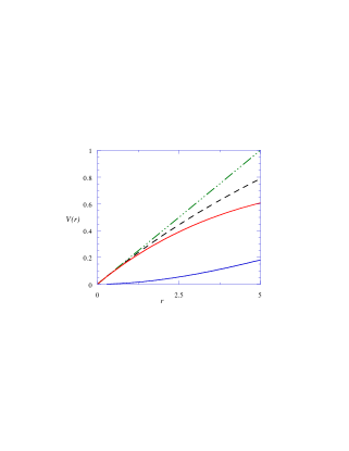
FIG. 2.: The potentials $\tilde{V}_{S}(r)$ (upper solid line), $\tilde{V}_{L}(r)$ (dashed line), $\sigma r$ (dot-dashed line), and $\tilde{V}_{0}(r)$ (lower solid line) in coordinate space for $\epsilon=0.1$ and $\sigma=0.2$.

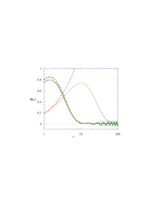
FIG. 3.: Comparison of possible wave functions $\Psi_{A}(r)$ (falling dotted line) and $\Psi_{S}(r)$ (heavy solid line). [For reference, the potentials $\tilde{V}_{S}(r)$ (thin solid line) and $\tilde{V}_{L}(r)$ (rising dotted line) are also shown.] The normalization is chosen so that $\Psi_{A}\leftrightarrow\Psi_{S}$, making the plane wave tail of $\Psi_{S}$ (shown in the box) small. In this example $\eta\simeq 0.05$.

In connection with the scattering form (18) we introduce a scattering state wave function defined by

$$\Psi_{S}({\bf p},p_{0})=(2\pi)^{3}\,\eta\;\delta^{3}(p-p^{\prime})-\frac{2m_{R}\,{M}_{S}({\bf p},{\bf p}^{\prime})}{{\bf p}^{2}-p_{0}^{2}}\,,$$ (20)

where ${M}_{S}$ is the half off-shell scattering amplitude, and ${\bf p}^{\prime 2}=p_{0}^{2}$. The wave function (20) has the form of the usual scattering wave function, with the $\delta$ function describing the asymptotic plane-wave part. We have chosen to multiply this plane-wave part by a (small) parameter $\eta$. This parameter can be removed by dividing the wave function and the half off-shell scattering amplitude by $\eta$, so it is, strictly speaking, an arbitrary scale factor. However, if we wish to compare the scattering solutions to (18) with the bound state solutions to (14), it is necessary to choose $\eta$ so that the wave functions are comparable at small $r$, as illustrated in Fig. 3, and this will require that $\eta$ be very small. Such a comparison is only possible at certain energies (close to the bound state energies) where the scattering solutions are resonant and therefore much larger at small $r$ than at large $r$. In general, at other energies, Eq. (18) will have nonresonant solutions that can not be large at small $r$. Only the resonant solutions of the scattering form (18) will converge to the bound state solutions to Eq. (14), and for these $\eta$ is very small. The non-resonant solutions to the scattering form are confined to the large $r$ region, and move off to infinity as $\epsilon\to 0$. This complicated limiting process will be summarized by the equation

$$\Psi_{S}({\bf p},p_{0})\leftrightarrow\Psi_{A}({\bf p},p_{0})\,,$$ (21)

where the $\leftrightarrow$ symbol means that the spectrum of resonance scattering states obtained from (18) converge to the bound states obtained from (14), and the nonresonant solutions to (18) can be ignored because they contribute only at infinite energy.

With this insight, we substitute the scattering wave function (20) into the Schrödinger equation (14), giving

$${M}_{S}({\bf p},{\bf p}^{\prime}) =\eta\,V_{S}({\bf p}-{\bf p}^{\prime})-2m_{R}\int\frac{d^{3}k}{(2\pi)^{3}}V_{S}({\bf p}-{\bf k})\,\frac{{M}_{S}({\bf k},{\bf p}^{\prime})}{{\bf k}^{2}-p_{0}^{2}}\,.$$ (22)

Alternatively, we may work directly with the bound state form (14) of the equation. In this case we make the replacement

$$\Psi_{A}({\bf p},p_{0})=-\frac{2m_{R}\,M_{A}({\bf p},{\bf p}^{\prime})}{{\bf p}^{2}-p_{0}^{2}}$$ (23)

and, substituting this into Eq. (14), obtain the following equation

$${M}_{A}({\bf p},{\bf p}^{\prime})=-2m_{R}\int\frac{d^{3}k}{(2\pi)^{3}}V_{A}({\bf p}-{\bf k})\,\left[\frac{{M}_{A}({\bf k},{\bf p}^{\prime})}{{\bf k}^{2}-p_{0}^{2}}-\frac{{M}_{A}({\bf p},{\bf p}^{\prime})}{{\bf p}^{2}-p_{0}^{2}}\right]\,.$$ (24)

Following the argument developed above, in the limit $\epsilon\to 0$ (and $\eta\to 0$) the two amplitudes $M_{S}$ and $M_{A}$ should be equivalent. In the notation of Eq. (21)

$$M_{S}({\bf p},{\bf p}^{\prime})\leftrightarrow M_{A}({\bf p},{\bf p}^{\prime})\,.$$ (25)

We will find it convenient to use $M_{S}$ when $\epsilon$ is very small but nonzero, and to use $M_{A}$ when we want exact confinement ($\epsilon=0$). Only Eq. (24) has a well defined mathematical limit when $\epsilon\to 0$. In our subsequent development we will assume that either $M_{S}$ or $M_{A}$ may be used with equivalent results.

When $\epsilon=0$, the inhomogeneous term vanishes and there exist bound states only. We introduce the vertex function $\gamma$ defined by

$$\Psi_{A}({\bf p},p_{0})=-\frac{2m_{R}\,{\gamma}({\bf p},p_{0})}{{\bf p}^{2}-p_{0}^{2}}\,.$$ (26)

The Schrödinger equation for the vertex function, restoring the constant interaction term, is

$$\gamma({\bf p},p_{0})=-2m_{R}\int\frac{d^{3}k}{(2\pi)^{3}}V_{A}({\bf p}-{\bf k})\,\left[\frac{\gamma({\bf k},p_{0})}{{\bf k}^{2}-p_{0}^{2}}-\frac{\gamma({\bf p},p_{0})}{{\bf p}^{2}-p_{0}^{2}}\right]+\frac{2m_{R}C\,\gamma({\bf p},p_{0})}{{\bf p}^{2}-p_{0}^{2}}\,.$$ (27)

Next, look at this equation when ${\bf p}^{2}\to p_{0}^{2}$. To this end first write

$${\gamma}({\bf p},p_{0})={\gamma}(p_{0},p_{0})+({\bf p}^{2}-p_{0}^{2})\,{\cal R}({\bf p},p_{0})\,,$$ (28)

and then substitute this into Eq. (27) [with $C=0$ for the moment], giving

$${\gamma}({\bf p},p_{0})= -2m_{R}\,{\gamma}(p_{0},p_{0})\int\frac{d^{3}k}{(2\pi)^{3}}V_{A}({\bf p}-{\bf k})\,\left[\frac{1}{{\bf k}^{2}-p_{0}^{2}}-\frac{1}{{\bf p}^{2}-p_{0}^{2}}\right]$$ (30)

$$-2m_{R}\int\frac{d^{3}k}{(2\pi)^{3}}V_{A}({\bf p}-{\bf k})\,\left[{\cal R}({\bf k},p_{0})-{\cal R}({\bf p},p_{0})\right]\,.$$

All terms on the r.h.s. of this equation should be regular as ${\bf p}^{2}\to p_{0}^{2}$. Because of the subtraction, the term involving ${\cal R}$ is finite, and, because of our choice of $p_{0}$, only one of the two remaining terms is zero if $\epsilon$ is finite

$$\lim_{{\bf p}^{2}\to p_{0}^{2}}\int\frac{d^{3}k}{(2\pi)^{3}}\frac{V_{A}({\bf p}-{\bf k})}{{\bf k}^{2}-p_{0}^{2}}= -\frac{\sigma}{\epsilon^{2}}\left(\frac{\epsilon\pm 2ip_{0}}{4p_{0}^{2}+\epsilon^{2}}\right)\to{\rm finite}$$ (31)

$$\lim_{{\bf p}^{2}\to p_{0}^{2}}\int\frac{d^{3}k}{(2\pi)^{3}}\frac{V_{A}({\bf p}-{\bf k})}{{\bf p}^{2}-p_{0}^{2}}= -\frac{\sigma}{\epsilon}\,\lim_{{\bf p}^{2}\to p_{0}^{2}}\left(\frac{1}{{\bf p}^{2}-p_{0}^{2}}\right)\to\infty\,.$$ (32)

Hence the subtraction term will be singular unless

$${\gamma}(p_{0},p_{0})=0\,.$$ (33)

This condition also insures that the constant term is not singular. We will discuss the physical interpretation of this result in the next section.

III Confinement in the spectator formalism

A Introduction

At this point it is very tempting to generalize the nonrelativistic linear potential Eq. (3) by simply replacing the three vector ${\bf q}$ by a four vector $q$

$${\cal V}({\bf q})\stackrel{{\scriptstyle?}}{{\rightarrow}}\lim_{\epsilon\rightarrow 0}\Bigl{[}V_{A}(q)-\delta^{4}(q)\int d^{4}q^{\prime}V_{A}(q^{\prime})\Bigr{]}+(2\pi)^{3}\delta^{4}(q)C.$$ (34)

This, seemingly obvious, generalization will not reduce to the correct nonrelativistic limit because of the unconstrained behavior of the $\int dq_{0}^{\prime}\,V_{A}(q^{\prime})$ integral. Lacking a four dimensional expression for the linear interaction that reduces to the correct nonrelativistic limit, we rephrase our question: Can one find a covariant equation that reduces to the Schrödinger Eq. (27) with a linear interaction? The confining relativistic bound state equation should be a relativistic generalization of Eq. (27).

FIG. 4.: One of the two-channel Gross equations for the bound state vertex function $\Gamma$. In this figure the $\times$ means that the particle is on the mass-shell.

A covariant equation with the correct nonrelativistic limit is the Gross equation[5, 6]. If the two quarks have unequal masses $m_{1}>m_{2}$, the one channel equation may be used. It has the feature that the four dimensional loop integrals are constrained so that the heavier constituent (with mass $m_{1}$ in this example) is restricted to its positive-energy mass shell (provided $M_{B}>0$; see Ref. [7]). However, if the particles have equal mass ($m_{1}=m_{2}=m$) and the mass $M_{B}$ of the bound state is comparable to $m$, a symmetrized two channel equation should be used. This is illustrated in Fig 4. In this case an average of the contributions in which either particle 1 (channel 1) or particle 2 (channel 2) are on their positive-energy mass-shell are included, and this leads to a set of equations in which the two channels are coupled. The symmetrized two-channel equation has been used previously to describe of low energy $NN$ scattering[8]. Finally, if the masses are identical and the bound state mass is very small (ie. $M_{B}<<m$), as in the chiral limit, then a four channel equation is needed. The four channel equation is a symmetrized version of the unsymmetrized two channel equation used in Ref.[1]. One of the purposes of this paper is to improve on this previous work.

B One channel scattering equations for scalar quarks

We will begin with the one channel equation. The momentum and mass of the quark are $p_{1}$ and $m_{1}$, the momentum and mass of the antiquark are $p_{2}$ and $m_{2}$, the total momentum is $P$, and the relative momentum is $p$, where

$$P= p_{1}+p_{2}=\{M_{B},{\bf 0}\}$$ (35)

$$p= {\frac{1}{2}}\left(p_{1}-p_{2}\right)\,.$$ (36)

The quark will be on mass-shell, and the symbol ${p}_{1}^{+}$ will be used to denote the particle on its positive energy mass-shell, (ie. ${p}_{1}^{+\,2}=m_{1}^{2}$ and $({p_{1}^{+}})_{0}=E_{1}(p)=\sqrt{m_{1}^{2}+{\bf p}^{2}}$). The scattering amplitude ${\cal M}({p}^{+}_{1},p_{2},{p}^{\prime+}_{1},p^{\prime}_{2})$ is denoted ${\cal M}_{11}({\bf p},{\bf p}^{\prime},P)$, or in the one channel case where there can be no confusion, simply by ${\cal M}({\bf p},{\bf p}^{\prime},P)$. Then, introducing a relativistic generalization of the potential $V_{S}$, the one channel equation for the scattering of scalar “quarks” ($m_{1}>m_{2}$) can be written

$${\cal M}_{S}({\bf p},{\bf p}^{\prime},P)= \eta V_{S}({\bf p},{\bf p}^{\prime},P)-\frac{2m_{1}m_{2}}{(2\pi)^{3}}\int\frac{d^{3}k}{E_{1}(k)}\;\frac{V_{S}({\bf p},{\bf k},P)\,{\cal M}_{S}({\bf k},{\bf p}^{\prime},P)}{m_{2}^{2}-(P-{k}^{+}_{1})^{2}}$$ (38)

$$+\frac{2m_{2}C\,{\cal M}_{S}({\bf p},{\bf p}^{\prime},p)}{m_{2}^{2}-(P-{p}^{+}_{1})^{2}}\,.$$

This equation is the relativistic generalization of Eq. (22).

Alternatively, the bound state form of the scattering equation is

$${\cal M}_{A}({\bf p},{\bf p}^{\prime},P)= -\frac{2m_{1}m_{2}}{(2\pi)^{3}}\int\frac{d^{3}k}{E_{1}(k)}V_{A}({\bf p},{\bf k},P)\;\left[\frac{{\cal M}_{A}({\bf k},{\bf p}^{\prime},P)}{m_{2}^{2}-(P-{k}^{+}_{1})^{2}}-\frac{{\cal M}_{A}({\bf p},{\bf p}^{\prime},P)}{m_{2}^{2}-(P-{p}^{+}_{1})^{2}}\right]$$ (40)

$$+\frac{2m_{2}C\,{\cal M}_{A}({\bf p},{\bf p}^{\prime},P)}{m_{2}^{2}-(P-{p}^{+}_{1})^{2}}\,.$$

This is the analogue of Eq. (24) and has a smooth limit as $\epsilon\to 0$. The kernels $V_{S}$ and $V_{A}$ will be specified later (see Eqs. (57) and (58) below). Equations (38) and (40) will be our starting points for this section.

C One channel bound state equation for scalar quarks

In the vicinity of a bound state of mass $M_{B}$, or a very narrow resonance with mass and width $M_{B}=M_{R}+iM_{I}$, the scattering amplitude has the form

$${\cal M}_{X}({\bf p},{\bf p}^{\prime},P)=-\frac{\Gamma_{X}({\bf p},M_{B})\,\Gamma_{X}({\bf p}^{\prime},M_{B})}{M_{B}^{2}-P^{2}}+{\cal R}_{X}({\bf p},M_{B})\,,$$ (41)

where $X=A$ or $S$, depending which of the two forms (38) or (40) we are using. If $\epsilon$ is finite and we are using Eq. (38), the width $M_{I}\neq 0$. If we use Eq. (38) the width is zero for all states with mass below some critical mass $M_{\epsilon}\to\infty$ as $\epsilon\to 0$.

Substituting the form (41) into either Eq. (38) or Eq. (40), and equating residues at the pole (real or complex) gives the bound state equations for the vertex functions $\Gamma_{X}$:

$$\Gamma_{S}({\bf p},M_{B})=-2m_{1}m_{2} \int\frac{d^{3}k\;V_{S}({p},{k},M_{B})}{(2\pi)^{3}\,E_{1}(k)}\frac{\Gamma_{S}({\bf k},M_{B})}{m_{2}^{2}-(M_{B}-{k}^{+}_{1})^{2}}$$ (43)

$$+\frac{2m_{2}\,C\,\Gamma_{S}({\bf p},M_{B})}{m_{2}^{2}-(M_{B}-{p}^{+}_{1})^{2}}\,,$$

$$\Gamma_{A}({\bf p},M_{B})=-2m_{1}m_{2} \int\frac{d^{3}k\;V_{A}({p},{k},M_{B})}{(2\pi)^{3}\,E_{1}(k)}\left[\frac{\Gamma_{A}({\bf k},M_{B})}{m_{2}^{2}-(M_{B}-{k}^{+}_{1})^{2}}-\frac{\Gamma_{A}({\bf p},M_{B})}{m_{2}^{2}-(M_{B}-{p}^{+}_{1})^{2}}\right]$$ (45)

$$+\frac{2m_{2}\,C\,\Gamma_{A}({\bf p},M_{B})}{m_{2}^{2}-(M_{B}-{p}^{+}_{1})^{2}}\,.$$

where we use a mixed notation with $M_{B}$ denoting both the mass and the four vector $\{M_{B},0\}$, the difference being clear from the context.

As with the scattering amplitudes, the two vertex functions are equivalent in the limit $\epsilon\to 0$

$$\Gamma_{S}({\bf p},M_{B})\leftrightarrow\Gamma_{A}({\bf p},M_{B})\,,$$ (46)

but the vertex function $\Gamma_{A}$ is more convenient to calculate in the limit $\epsilon\to 0$.

D Normalization condition

The bound state equation and the normalization condition for the bound state wave function can be derived from a nonlinear form of Eq. (38)[9]. In this paper the derivative $\partial V_{S}/\partial P_{\mu}=0$ in the rest frame, so the result is

$$2P^{\mu}=\frac{\partial}{\partial P_{\mu}}\int\frac{d^{3}k}{(2\pi)^{3}\,E_{1}(k)}\left\{\frac{\Gamma_{S}({\bf k},M_{B})\,\Gamma_{S}({\bf k},M_{B})}{m_{2}^{2}-(P-{k}^{+}_{1})^{2}}\right\}\,.$$ (47)

In view of the relation (46) this relation can also be written

$$2P^{\mu}= \frac{\partial}{\partial P_{\mu}}\int\frac{d^{3}k}{(2\pi)^{3}\,E_{1}(k)}\left\{\frac{{\Gamma}_{A}({\bf k},M_{B})\,{\Gamma}_{A}({\bf k},M_{B})}{m_{2}^{2}-(P-{k}^{+}_{1})^{2}}\right\}$$ (48)

$$= \int\frac{d^{3}k}{(2\pi)^{3}\,E_{1}(k)}\frac{{\Gamma}_{A}({\bf k},M_{B})\,2(P-{k}^{+}_{1})^{\mu}\,{\Gamma}_{A}({\bf k},M_{B})}{\left(m_{2}^{2}-(P-{k}^{+}_{1})^{2}\right)^{2}}\,.$$ (49)

This is a familiar result, which will be generalized to the spin 1/2 case later.

E Symmetrized two channel equation for equal mass scalar quarks

If the quarks have equal mass ($m_{1}=m_{2}=m$), and the bound state mass is positive and not too small, a symmetrized two channel equation is needed. The two channels will be labeled 1 and 2 depending on whether the quark or antiquark is on mass-shell, and the symbol ${p}_{1}^{+}$ denotes that the particle is on its positive energy mass-shell, (ie. ${p}_{1}^{+\,2}=m^{2}$ and ${p_{0}^{+}}=E(p)=\sqrt{m^{2}+{\bf p}^{2}}$). Starting from Eq.(45), and suppressing the subscript $A$, the vertex functions for the two channels are denoted

$$\Gamma_{1}({\bf p},M_{B})=\Gamma({p}^{+}_{1},p_{2}),\qquad\Gamma_{2}({\bf p},M_{B})\equiv\Gamma(p_{1},{p}^{+}_{2})\,.$$ (50)

With this notation, the symmetrized two channel equation for equal mass scalar “quarks” with a confining interaction can be written

$$\Gamma_{i}({\bf p},M_{B})=-m^{2} \sum_{j}\int\frac{d^{3}k\;V_{ij}({p},{k})}{(2\pi)^{3}\,E_{j}(k)}\left[\frac{\Gamma_{j}({\bf k},M_{B})}{m^{2}-(P-{k}^{+}_{j})^{2}}-\frac{\Gamma_{i}({\bf p},M_{B})}{m^{2}-(P-{p}^{+}_{i})^{2}}\right]$$ (52)

$$+\frac{2mC\,\Gamma_{i}({\bf p},M_{B})}{m^{2}-(P-{p}^{+}_{i})^{2}}\,,$$

where $i$ and $j$ label which of the two quarks is on-shell, and

$${k}^{+}_{j}=\{E(k),(-)^{j+1}\,{\bf k}\}$$ (53)

is the momentum of the on-shell quark. Note that the strength of the $V_{ij}$ term has been multiplied by 1/2, reflecting the fact that the interaction is an average of the strengths in two channels which are equal in the nonrelativistic limit. This equation uses the same subtraction for both the $i=j$ and the $i\neq j$ terms. This prescription differs from that previously used in Ref.[1]. In this work the kernel below will not, in general, be singular when $i\neq j$, and the subtraction used above is sufficient to preserve the nonrelativistic limit (see below).

In order to complete the description we need to specify the form of covariant interaction $V_{ij}$. A natural choice that reduces to the correct nonrelativistic limit is [1]

$$V_{ij}({p},{k})\equiv V_{A}(q_{ij})=-\frac{8\pi\sigma}{(q_{ij}^{2}-\epsilon^{2})^{2}}\,,$$ (54)

where the four-momentum transfer depends on whether or not $i=j$:

$$q_{11}^{2}= q_{22}^{2}=\left(E(k)-E(p)\right)^{2}-({\bf k}-{\bf p})^{2}$$ (55)

$$q_{12}^{2}= q_{21}^{2}=\left(M_{B}-E(k)-E(p)\right)^{2}-({\bf k}+{\bf p})^{2}\,.$$ (56)

A similar form could be used for the kernel $V_{S}$ (which we will not need)

$$V_{ij}({p},{k})\equiv V_{S}(q_{ij})=-8\pi\sigma\left\{\frac{1}{(q_{ij}^{2}-\epsilon^{2})^{2}}+\frac{4\epsilon^{2}}{(q_{ij}^{2}-\epsilon^{2})^{3}}\right\}\,.$$ (57)

However, the form (54) has two drawbacks. First, at large ${\bf p}\simeq{\bf k}$ the kernel converges slowly, and the equation is ultraviolet divergent. In Ref. [1] a form factor was introduced to regularize this divergence. Second, using this form it is difficult to regularize the infrared ($q^{2}=0$) singularities that appear in the $\epsilon=0$ limit. In the nonrelativistic case the infrared singularity occurs only at ${\bf q}=0$ and can be regulated by the $\delta$ function subtraction in Eq. (3). However, in the relativistic case infrared singularities occur not only when $q^{\mu}=0$, but also (for the $i\neq j$ kernels) when the momentum transfer is light-like, so that $q^{2}=0$ but $q^{\mu}\neq 0$. These “off-diagonal” singularities are not regulated by the subtraction term, and their removal spoils the simplicity of this approach[1].

Since the role of $V_{A}$ is to model the linear interaction, and the principle requirement is that it reduce to the correct nonrelativistic limit, both of these problems are eliminated very simply if $V_{A}$ is defined as follows

$$V_{A}(q_{ij})=-\frac{8\pi\sigma}{q_{ij}^{4}+(P\cdot q_{ij})^{4}/P^{4}}$$ (58)

where $P$ is the total four-momentum of the bound state. This form has the following advantages:

(i) the denominator is not singular unless both $q^{2}$ and $P\cdot q$ are zero, so the singularities are restricted to $q^{\mu}=0$;

(ii) no ultraviolet regularization is needed;

(iii) the interaction does not depend on the bound state momentum $P$ in the bound state rest frame; and

(iv) it has the correct nonrelativistic dependence on ${\bf q}^{2}$.

One disadvantage of the form (58) is its dependence on the total momentum $P$ of the particle pair. However, since since this kernel confines particles in pairs that can not be separated, they are naturally associated as a pair and we do not view this as a serious limitation. Another feature of the form (58) is that its off-diagonal couplings are singular only when $W=2E(p)$ (because ${\bf k}+{\bf p}=0$ also). This is only possible for excited states and, as we will prove below, confinement requires the vertex function to be zero at this point, controlling this singularity automatically.

The introduction of the definition (58) considerably simplifies the solution of the relativistic equations (52), but will introduce electromagnetic interaction currents if the photon four-momentum is not zero. These will be discussed in a subsequent paper.

Both Eqs. (45) and (52) have the correct nonrelativistic limit with confinement. Consider the one-channel Eq. (45) first, and let $m_{1}$ and $m_{2}\to\infty$. Then the energy transferred by the on-shell quark, $E_{1}(k)-E_{1}(p)\to 0$ and $V_{A}(q_{11})\to V_{A}({\bf q})$. Furthermore, if $M_{B}=m_{2}+m_{1}+E$, then to first order in the small quantities ${\bf k}^{2}$ and $m_{R}E$, the relativistic propagator reduces to

$$\frac{1}{m_{2}^{2}-k_{2}^{2}}\to\frac{m_{R}}{m_{2}({\bf k}^{2}-2m_{R}E)}\,,$$ (59)

and substituting this into Eq. (45) gives Eq. (27). In the two channel case $q_{11}\to q_{12}$ as $m\to\infty$ and the kernels $V_{11}\to V_{12}$. Since the subtraction in the two channels is also identical, the contributions from the two channels are equal and the coupled equations reduce to the single Eq. (27).

F Proof of confinement

While one can visualize the potential in the nonrelativistic case and get a picture of the physics, it is less possible to visualize the covariant interaction. What are the criteria with which one can judge whether a given interaction really confines? If the particles are bound in a state of total mass larger than the sum of the masses of the constituents ($M_{B}>m_{1}+m_{2}$), the bound state could in principle decay into free constituents. Confinement prevents this from happening in one of two possible ways: (i) the quark propagators will not have any physical mass poles [10], or, as we will now prove for this model, (ii) the vertex function will vanish when the quarks are simultaneously on-shell.

The proof is identical to the nonrelativistic proof given above and we will summarize it only for the one channel equation. Setting $C=0$, the one channel bound state Eq. (45) can be written

$$\Gamma_{A}({\bf p},M_{B})= -2m_{1}m_{2}\int\frac{d^{3}k\;V_{A}(p,k)}{(2\pi)^{3}\,E_{1}(k)}\left[\frac{\Gamma_{A}({\bf k},M_{B})-\Gamma_{A}({\bf p},M_{B})}{m_{2}^{2}-k_{2}^{2}}\right]$$ (61)

$$+2m_{1}m_{2}\Gamma_{A}({\bf p},M_{B})\int\frac{d^{3}k\;V_{A}(p,k)}{(2\pi)^{3}\,E_{1}(k)}\left\{\frac{p_{2}^{2}-k_{2}^{2}}{\left(m_{2}^{2}-p_{2}^{2}\right)\left(m_{2}^{2}-k_{2}^{2}\right)}\right\}\,.$$

Since the first quark is on-shell, the second quark is on its positive energy mass shell when the magnitude of the relative three-momentum $|{\bf p}|={p}_{0}$ is

$$\sqrt{m_{1}^{2}+{p}_{0}^{2}}+\sqrt{m_{2}^{2}+{p}_{0}^{2}}=M_{B}\,.$$ (62)

This occurs when ${p}_{0}^{2}$ is given by

$$4M_{B}^{2}\,{p}_{0}^{2}=\left[M_{B}^{2}-(m_{1}+m_{2})^{2}\right]\left[M_{B}^{2}-(m_{1}-m_{2})^{2}\right]\,.$$ (63)

As in the nonrelativistic case, the singularity at ${\bf p}={\bf k}$ is integrable, and hence the second term on r.h.s. of Eq. (61) will be singular at ${\bf p}={p}_{0}\,{\bf\hat{p}}\equiv{\bf p}_{0}$ (where ${\bf\hat{p}}$ is a unit vector in the direction of ${\bf p}$) unless

$$\Gamma({\bf p}_{0},M_{B})=0\,.$$ (64)

Therefore, the vertex function vanishes when both particles are on their mass shell. This condition is illustrated diagrammatically in Fig. 5.

Note that the subtraction term in Eqs. (52) and (61) plays two central roles: (i) it regularizes the singular interaction at ${\bf p}={\bf k}$ and and makes it zero at $r=0$, and (ii) it is singular when $p_{2}^{2}\to m_{2}^{2}$, forcing condition (64). The subtraction term is essential to the self consistent description of confinement. As in the nonrelativistic case the proof did not depend on the specific form of the interaction.

FIG. 5.: The confinement condition for the Gross vertex function.

We now discuss how confinement affects the stability of bound states under external disturbances.

G Excitation of bound states

A consistent description of confinement implies that two free quarks can not be liberated from a bound state, even under the influence of an energetic external photon or other probe. This requirement implies that the usual Born term (shown in Fig. 6) is either cancelled by the rescattering term, or is a diagram that does not exist in the formalism. If the Born term does not exist, the rescattering term, illustrated in Fig 7, must be zero if the final state quarks are all on-shell. How are these restrictions built into the formalism?

When particles are confined there are no free two-particle states and the two-body propagator must always include an infinite number of interactions. Since there are no free particle states, a perturbation theory for confined particles built around the free propagator can not be constructed. This feature is built-in automatically if the two body propagators satisfy homogeneous integral equations with no free particle contribution.

To illustrate these ideas we review the formalism for the scattering amplitude, and its relation to the two-body propagator. It is convenient to work with the scattering form of the equation. In operator notation, Eq.(18) is:

$$M({\bf p},{\bf p}^{\prime},P)= \eta\,V(p,p^{\prime})-V(p,k)G_{0}({\bf k},{\bf k}^{\prime},P)M({\bf k}^{\prime},{\bf p}^{\prime},P)$$ (65)

$$= \eta\,V(p,p^{\prime})-M({\bf p},{\bf k},P)G_{0}({\bf k},{\bf k}^{\prime},P)V(k^{\prime},p^{\prime})\,,$$ (66)

where $G_{0}({\bf k},{\bf k}^{\prime},P)$ is the free two body propagator [containing a factor of $\delta^{3}(k-k^{\prime})$], integration over $d^{3}k$ and $d^{3}k^{\prime}$ is implied, and we have dropped the subscript $S$ for simplicity. The parameter $\eta$ was introduced in the discussion following Eq.(20) and is very small, approaching zero as $\epsilon\to 0$.

FIG. 6.: The Born term, which can not exist if the quarks are confined.

FIG. 7.: Can an external photon probe disintegrate the bound state?

Now the dressed propagator, $G$ is related to the scattering amplitude $M$ by

$$G({\bf p},{\bf p}^{\prime},P)= \zeta\,G_{0}({\bf p},{\bf p}^{\prime},P)-G_{0}({\bf p},{\bf k},P)M({\bf k},{\bf k}^{\prime},P)G_{0}({\bf k}^{\prime},{\bf p}^{\prime},P)\,,$$ (67)

where $\zeta$, to be determined, is a parameter proportional to the strength of the free particle scattering. If the potential confines there should be no inhomogeneous term and $\zeta=0$. To determine $\zeta$ and the equation for $G$, substitute (66) into (67) giving

$$G({\bf p},{\bf p}^{\prime},P)= \zeta\,G_{0}({\bf p},{\bf p}^{\prime},P)-\eta G_{0}({\bf p},{\bf k},P)V(k,k^{\prime})G_{0}({\bf k}^{\prime},{\bf p}^{\prime},P)$$ (69)

$$+G_{0}({\bf p},{\bf k},P)V(k,k^{\prime})G_{0}({\bf k^{\prime}},{\bf k}^{\prime\prime},P)M({\bf k}^{\prime\prime},{\bf k}^{\prime\prime\prime},P)G_{0}({\bf k}^{\prime\prime\prime},{\bf p}^{\prime},P)$$

$$= \zeta\,G_{0}({\bf p},{\bf p}^{\prime},P)+(\zeta-\eta)\,G_{0}({\bf p},{\bf k},P)V(k,k^{\prime})G_{0}({\bf k}^{\prime},{\bf p}^{\prime},P)$$ (71)

$$-G_{0}({\bf p},{\bf k},P)V(k,k^{\prime})G({\bf k^{\prime}},{\bf p}^{\prime},P)\,.$$

The second term is eliminated by choosing $\zeta=\eta$, and gives familiar equations for the dressed propagator

$$G({\bf p},{\bf p}^{\prime},P)= \eta\,G_{0}({\bf p},{\bf p}^{\prime},P)-G_{0}({\bf p},{\bf k},P)V(k,k^{\prime})G({\bf k}^{\prime},{\bf p}^{\prime},P)$$ (72)

$$= \eta\,G_{0}({\bf p},{\bf p}^{\prime},P)-G({\bf p},{\bf k},P)V(k,k^{\prime})G_{0}({\bf k}^{\prime},{\bf p}^{\prime},P)\,,$$ (73)

where the second form parallels the second form of Eq. (66).

The interpretation of equations (67) and (73) for the dressed propagator follows from the interpretation of Eq. (66) for the scattering amplitude. As $\epsilon\to 0$, the parameter $\eta\to 0$ and the inhomogeneous term vanishes. In this limit both the scattering amplitude and the propagator satisfy homogeneous equations.

The inelastic scattering amplitude can be obtained from the dressed propagator by striping off the final free propagators, and is [6]

$${\cal J}({\bf p},P,q)= G_{0}^{-1}({\bf p},{\bf k},P+q)G({\bf k},{\bf p}^{\prime},P+q)J(P+q,P)\Psi(P)$$ (74)

$$= \Bigl{\{}\eta+M({\bf p},{\bf k},P+q)G_{0}({\bf k},{\bf p}^{\prime},P+q)\Bigr{\}}\,J(P+q,P)\Psi(P)\,.$$ (75)

Here the first term proportional to $\eta$ is the Born term shown in Fig. 6, and we see that there is no Born term in the limit of exact confinement (ie. $\eta=0$). Furthermore, in the presence of confinement the scattering matrix satisfies the same homogeneous equation satisfied by the bound states [Eq. (66) with $\eta=0$], and an extension of the proof given in Subsec. F above shows that the scattering matrix in Fig. 7 must be zero if both final state quarks are on shell.

We have constructed a self-consistent description of confinement within the context of relativistic field theory.

H Generalization to Fermions

If the quarks have spin, the kernel in the spectator equation will be an operator in the Dirac space of the two quarks. This operator can be written

$${\cal V}(p,k)=\sum_{i=1}^{3}\alpha_{i}\,O_{i1}\,O_{i2}\;V_{i}(p,k)\,,$$ (76)

where the Dirac matrices $O$, which operate on the Dirac indices of particles 1 and 2, describe the spin dependent structure of quark-antiquark interaction. The $\alpha_{i}$ are parameters determined either empirically (by fitting the spectrum), from lattice calculations, or from the theory. In this paper we consider only three possible spin structures: scalar $O_{1j}=\openone_{j}$, pseudoscalar $O_{2j}=\gamma_{5j}$, and vector $O_{3j}=\gamma_{\mu j}/{2}$. With this notation the one channel spectator equation for spin 1/2 particles with constant masses $m_{1}>>m_{2}$ is given by

$$\Gamma(p,P)=-\int\frac{d^{3}k}{(2\pi)^{3}E_{1}(k)}\,\sum_{i}V_{i}(p,k)O_{i1}(m_{1}+{\ \!/\!\!\!\!k}^{+}_{1})\left\{\frac{\Gamma(k,P)}{m_{2}^{2}-k_{2}^{2}}\right\}(m_{2}-\ \!/\!\!\!\!k_{2})O_{i2},$$ (77)

where the quark has mass $m_{1}$ and is on shell, so that ${k}_{1}^{+\,2}=m_{1}^{2}={p}_{1}^{+\,2}$, and the antiquark has mass $m_{2}$. Therefore, the momentum transfered by the interaction is

$$({p}^{+}-{k}^{+})^{2}=(E_{1}(p)-E_{1}(k))^{2}-({\bf p}-{\bf k})^{2}\equiv q\,.$$ (78)

As in the nonrelativistic case, we consider a kernel composed of linear, constant, and one gluon exchange (OGE) pieces. The interaction kernel for the linear part of the potential, ${\cal V}_{L}$, is

$${\cal V}_{L}(p,k) \equiv \sum_{i=1}^{3}\alpha_{Li}\,O_{i1}\,O_{i2}V_{L}(p,k),$$ (79)

$$= \left(\alpha_{s}\openone_{1}\openone_{2}+\alpha_{ps}\gamma_{51}\gamma_{52}+{\frac{1}{4}}\,\alpha_{v}\,\gamma_{\mu 1}\gamma^{\mu}_{2}\right)\,V_{L}(p,k)\,,$$ (80)

where $V_{L}(p,k)$ is

$$V_{L}(p,k)=V_{A}(q_{11}(p,k))-E_{1}(k)\,\delta^{3}(p-k)\int d^{3}k^{\prime}\frac{V_{A}(q_{11}(p,k^{\prime}))}{E_{1}(k^{\prime})}\,.$$ (81)

In this work we employ a pure scalar linear interaction, $\alpha_{s}=1,\alpha_{ps}=\alpha_{v}=0$, but in later calculations the coefficients $\alpha_{i}$ will be determined empirically. The one gluon exchange and constant interactions will be pure vector

$${\cal V}_{g}(q) = \gamma_{\mu 1}\,\gamma_{\nu 2}\,V_{g}^{\mu\nu}(q)$$ (82)

$${\cal V}_{c}(q) = \gamma_{\mu 1}\,\gamma^{\mu}_{2}\,C\,,$$ (83)

where

$$V_{g}^{\mu\nu}(q) \equiv -(g^{\mu\nu}-\frac{q^{\mu}q^{\nu}}{q^{2}})\,V_{g}(q)$$ (84)

$$= -(g^{\mu\nu}-\frac{q^{\mu}q^{\nu}}{q^{2}})\,\frac{1}{q^{2}-\Lambda^{2}}\,\frac{d\;16\pi^{2}/3}{\ln(\tau+|q^{2}|/\lambda_{QCD}^{2})}\,,$$ (85)

where $d=12/(33-2N_{f})=12/27$, the color factor of 4/3 has been included, $\Lambda=1$ GeV, $\tau$ = 2, and $\lambda_{QCD}$ = 200 MeV. In previous work [1] quark propagators with constant masses were used. In this work we parametrize the quark propagator by

$$S(p)=\frac{1}{m(p)-\not\!p}\,,$$ (86)

where $m(p)$ is a mass function for the quark, to be defined later.

FIG. 8.: Propagator poles in the complex $k_{0}$ plane.

If the constituents are identical or close in mass and the equations are to be applied to the description of nearly massless bound states, the four channel equation should be used. Numerical solutions the four channel equation will be presented in this work.

The four channels are defined by the constraints in the four-momenta $k_{1}$ and $k_{2}$ arising from the requirement that both the quark and the antiquark be constrained to both their positive and negative energy mass-shells. A formal way to obtain the equations is to integrate over the internal energy $k_{0}$ by averaging the contributions from the quark and antiquark poles in both the upper and lower half $k_{0}$ complex plane, as illustrated in Fig. 8. This averaging is needed to ensure charge conjugation (particle-antiparticle) symmetry, and leads to four coupled equations. However, even though the form of the equations is obtained in this way, we emphasize that the equations are theoretically justified by the argument that the singularities in the interaction kernel omitted in this procedure tend to be cancelled by other higher order terms which would otherwise have been neglected, and that this leads to covariant equations with the correct nonrelativistic limit. The inclusion of the negative energy poles, neglected in other applications of the symmetrized equations[8], is required in cases where $P\to 0$[1].

The four constraints are conveniently identified by the notation

$${k}_{j}^{s}=\{sE(k),(-)^{j+1}\,{\bf k}\}\,.$$ (87)

which generalizes that introduced in Eq. (53). Here the superscript $s=\pm$ denotes either the positive or negative energy mass shell constraints. Then, introducing the projection operators

$$\Lambda(k)=m(k)+\ \!/\!\!\!\!k\,,$$ (88)

and defining the four channel vertex functions

$$\Gamma_{1}^{s}({\bf p},M_{B})= \Gamma(p_{1}^{s},p_{2})$$ (89)

$$\Gamma_{2}^{s}({\bf p},M_{B})= \Gamma(p_{1},p_{2}^{s})\,,$$ (90)

and wave functions

$$\Psi_{1}^{s}({\bf p},M_{B})= \frac{\Lambda(p_{1}^{s})\Gamma^{s}_{1}({\bf p},M_{B})\Lambda(-p_{2})}{m(p_{2})^{2}-p_{2}^{2}}$$ (91)

$$\Psi_{2}^{s}({\bf p},M_{B})= \frac{\Lambda(p_{1})\Gamma^{s}_{2}({\bf p},M_{B})\Lambda(-p_{2}^{s})}{m(p_{1})^{2}-p_{1}^{2}}\,,$$ (92)

permits us to write the four-channel spectator equation in the following compact form

$$\Gamma_{i}^{s}({\bf p},M_{B})= - \frac{1}{2}\sum_{jr}\int\frac{d^{3}k}{(2\pi)^{3}\,2E(k)}\Biggl{\{}V_{ij}^{sr}(p,k)\left[\Psi_{j}^{r}({\bf k},M_{B})-\Psi_{i}^{s}({\bf p},M_{B})\right]$$ (93)

$$- 2\delta_{ij}\delta_{sr}V_{g}^{\mu\nu}(p-k)\gamma_{\mu}\Psi_{j}^{r}({\bf k},M_{B})\gamma_{\nu}\Biggr{\}}-C\,\gamma_{\mu}\Psi_{i}^{s}({\bf p},M_{B})\gamma^{\mu}\,,$$ (94)

where the r.h.s. of the equation now sums over both positive and negative energy contributions ($r=\pm$) from each quark ($j=\pm$). The Kronecker $\delta_{ij}\delta_{sr}$ functions restrict the one gluon exchange interaction to the diagonal channels (where the same particle is on the same mass shell before and after the interaction). Inclusion of the one gluon exchange in off-diagonal channels leads to numerical instabilities, which in principle can be handled by using more grid points in numerical integrations. Restricting this interaction to diagonal channels eliminates these singularities from the gluon propagator.

I Charge conjugation invariance

The final task is to show that Eq. (94) is invariant under the charge conjugation operation

$$\Gamma^{\cal C}(p_{1},p_{2})={\cal C}\Gamma^{\rm T}(p_{2},p_{1}){\cal C}^{-1}\,.$$ (95)

This is done by proving that both $\Gamma$ and $\Gamma^{\cal C}$ satisfy the same equation.

First note that, when particle 1 is on shell, interchange of $p_{1}$ and $p_{2}$ gives

$$\Gamma_{1}^{s}({\bf p},M_{B})=\Gamma(p_{1}^{s},p_{2})\to\Gamma(p_{2},p_{1}^{s})=\Gamma_{2}^{s}(-{\bf p},M_{B})$$ (96)

and is equivalent to $1\leftrightarrow 2$ and ${\bf p}\to-{\bf p}$. Then

$$\Psi_{1}^{s\,{\cal C}}({\bf p},M_{B})= {\cal C}\Psi_{2}^{s\,{\rm T}}(-{\bf p},M_{B}){\cal C}^{-1}$$ (97)

$$\Psi_{2}^{s\,{\cal C}}({\bf p},M_{B})= {\cal C}\Psi_{1}^{s\,{\rm T}}(-{\bf p},M_{B}){\cal C}^{-1}\,.$$ (98)

Finally, the Dirac direct products $\openone\otimes\openone$, $\gamma_{\mu}\otimes\gamma^{\mu}$, and $\gamma_{5}\otimes\gamma_{5}$ are invariant under ${\cal C}$. Hence, changing ${\bf k}\to-{\bf k}$ and performing the transformations (95) and (96), shows that Eq. (94) is also invariant. Therefore the charge conjugation eigenstates, labeled by $\eta=\pm$

$$\Gamma_{\eta}^{s}({\bf p},M_{B})= \Gamma_{1}^{s}({\bf p},M_{B})+\eta\,\Gamma_{2}^{s\,{\cal C}}({\bf p},M_{B})\,,$$ (99)

are solutions of the equation and charge conjugation symmetry is proved.

J Dynamical quark mass

The dynamical quark mass function is the solution of the Dyson-Schwinger equation. In NJL-type models, this one-body equation for the spontaneous generation of quark mass and the two-body bound state equation for a state of zero mass become identical in the chiral limit (when the bare quark mass is zero). In this limit the quark mass function and the bound state wavefunction for a massless pseudoscalar bound state are identical, and spontaneous symmetry breaking assures the existance of a massless pseudoscalar bound state.

In this paper we adopt a slightly different approach. We will first choose a convenient mass function, and then require that the two-body equation for a massles pseudoscalar bound state automatically have a solution when the bare quark mass is zero. In this case the quark mass function and the wave function for the massless Goldstone boson will not be identical, but at least the existence of the Goldstone boson in the chiral limit is assured. We will define the quark mass function of flavor $f$ by

$$m_{f}(p)\equiv m_{f}^{0}+c(m_{f}^{0})\,f(p),$$ (100)

where $m_{f}^{0}$ is the current quark mass of flavor $f$, and $f(p)$ is a universal function defined by

$$f(p)\equiv\frac{1}{|p^{2}|+\Lambda^{2}}.$$ (101)

The function $c(m_{f}^{0})$ can be thought of as a polynomial in powers of $m_{f}^{0}$. This is the typical structure of the mass function which is usually obtained from the solution of the one body equation.

The reason for not solving the one body equation, in our case, is two fold. The first problem is the difficulty of incorporating one gluon exchange into the one body equation. Because of the on-shell constraint in the loop momenta, the one gluon exchange interaction leads to an ultraviolet divergence. The second problem is associated with our choice of infrared regularization of the linear interaction. The infrared singularities are regulated by the $P\cdot q$ term in the denominator of the linear interaction Eq. (58), and this would imply that the resultant mass function is a function of two arguments, i.e. $m=m(p^{2},{\bf p}^{2})$. This is unacceptable, and rather than forsaking important features of the model such as confinement and asymptotic freedom, we choose to model the quark mass functions.

The form (100) guarantees that at large momenta, quark masses go to their current quark mass values as dictated by asymptotic freedom. In the chiral limit the quark mass reduces to

$$m_{\chi}(p)=c(0)\,f(p)$$ (102)

We fix the constant $c(0)$ by requiring that the pion bound state equation, using the mass function (102), give a massles solution. This insures that a massless pion exists in the chiral limit when $m_{f}^{0}=0$. Next we choose a value for the light current quark mass, $m_{u}^{0}=m_{d}^{0}$, and fix $c(m_{u}^{0})$ so that the two-body equation gives the correct value for the physical pion mass. This also fixes the value of the on-shell quark mass away from the chiral limit. Similarly, we choose $m_{s}^{0}$ and fix $c(m_{s}^{0})$ by fitting the kaon mass. For three flavors it is therefore sufficient to have a function $c(m_{f}^{0})$ which is a polynomial of order 2 in $m_{f}^{0}$. As new flavors are introduced the order of the polynomial accordingly can be increased.

To summarize, we have 6 mass parameters: $m^{0}_{u},m^{0}_{s},c(0),c(m_{u}^{0}),c(m_{s}^{0})$, and $\Lambda$. In practice we fix $\Lambda$ at one GeV and choose the current quark masses $m^{0}_{u},$ and $m^{0}_{s}$ to be near the values expected by current theory. We then adjust the $c$’s to give the a zero mass pion in the chiral limit, and a real pion and kaon with the observed masses. This process is repeated for different values of the current quark masses and the potential parameters $\sigma$ and $C$ until satisfactory values for the constituent quark masses and the spectrum of excited pions is obtained. The final values of the parameters will be given in the next section.

Having outlined the features of the model, we now turn our attention to the details of the pseudoscalar bound state equation with spin.

IV Pseudoscalar channel

The bound state vertex function has the following structure

$$\chi=\chi_{\rm color}\otimes\chi_{\rm flavor}\otimes\chi_{\rm spin}.$$ (103)

The color space vertex function is a Kronecker delta function, $\delta_{cd}$, which reflects the color singlet nature of the bound state. The flavor space vertex function is the matrix $\lambda^{i}_{fg}$ in $SU(3)$ matrix space, which chooses the right flavor combination of the meson under consideration. Indices $f,g$ refer to up down and strange quark entries ($u,d,s=1,2,3$) of $\lambda^{i}$. For example, $[\lambda^{+}]_{ud}=[\lambda^{+}]_{12}$. For a general meson type $i$, the bound state vertex function is

$$\chi_{\alpha\beta,fg,cd}^{i}(k_{1},k_{2})\equiv\delta_{cd}\,\lambda^{i}_{fg}\,\Gamma_{\alpha\beta}(k_{1},k_{2}).$$ (104)

where $\alpha,\beta$ are Dirac indices (to be suppressed in the following discussion). The most general form for the spin-space part of the vertex function for pseudoscalar mesons is

$$\Gamma(k_{1},k_{2})=\gamma_{5}\bigg{\{}\Gamma_{0}+\ \!/\!\!\!\!P\,\Gamma_{1}+\ \!/\!\!\!k\,\Gamma_{2}+[\ \!/\!\!\!k,\ \!/\!\!\!\!P]\,\Gamma_{3}\bigg{\}}\,,$$ (105)

where $\Gamma_{i}=\Gamma_{i}(k_{1},k_{2})$ are scalar functions. The dominant contribution to the bound state vertex function comes from the first term of (105),

$$\Gamma(k_{1},k_{2})\approx\gamma_{5}\,\Gamma_{0}(k_{1},k_{2})\,,$$ (106)

This approximation, which is exact in the chiral limit when $P=0$ and $m_{1}=m_{2}$, will be used for the pion and kaon bound states in this work.

Assuming (106), multiplying the four channel equations for pseudoscalar mesons by $\gamma_{5}$, and taking the trace, gives the following approximate coupled equations for pseudoscalar states

$$\Gamma_{i}^{s}({\bf p},M_{B})= - \frac{1}{2}\sum_{jr}\int\frac{d^{3}k}{(2\pi)^{3}\,2E_{j}(k)}\Biggl{\{}V_{ij}^{sr}(p,k)\left[F_{j}(k_{j}^{r})\Gamma_{j}^{r}({\bf k},M_{B})-F_{i}(p_{i}^{s})\Gamma_{i}^{s}({\bf p},M_{B})\right]$$ (107)

$$+ 6\delta_{ij}\delta_{sr}V_{g}(p-k)F_{j}(k_{j}^{r})\Gamma_{j}^{r}({\bf k},M_{B})\Biggr{\}}+2F_{i}(p_{i}^{s})C\Gamma_{i}^{s}({\bf p},M_{B})\,,$$ (108)

where the four channel wave functions $\Gamma_{i}^{s}({\bf p},M_{B})$ are obtained from $\Gamma_{0}$ as shown in Eq. (90), and

$$F_{1}(k_{1}^{r})\equiv \frac{m_{1}m_{2}(k_{2})+k^{r}_{1}\cdot k_{2}}{m_{2}^{2}(k_{2})-k_{2}^{2}}$$ (109)

$$F_{2}(k_{2}^{r})\equiv \frac{m_{1}(k_{1})m_{2}+k_{1}\cdot k^{r}_{2}}{m^{2}_{1}(k_{2})-k_{1}^{2}}\,,$$ (110)

where $m_{i}(k_{i}^{r})=m_{i}(-k_{i}^{r})=m_{i}$. For future reference we record the four-momentum $q_{ij}^{rs}\equiv(p_{1}-k_{1})_{ij}^{rs}$ exchanged between the two quarks. This depends on the initial and final channel. The distinct cases are:

$$q_{11}^{rs} =q_{22}^{-r,-s}=(rE(p)-sE(k),\;{\bf p}-{\bf k})$$ (111)

$$q_{12}^{rs} =(rE(p)+sE(k)-M_{B},\;{\bf p}-{\bf k})$$ (112)

$$q_{21}^{rs} =(M_{B}-rE(p)-sE(k),\;{\bf p}-{\bf k})\,.$$ (113)

The solution of Eqs. (108) for a realistic choice of the parameters will be discussed in the next section.

Before turning to this discussion, look at the coupled equations in the chiral limit, when $P=0$ and the dynamical quark masses are equal, so that $m_{1}(k)=m_{2}(k)=m(k)$. In this limit, $k_{1}=-k_{2}$, and expanding to order $P\cdot k_{1}^{r}$ gives

$$F_{1}(k_{1}^{r})=\frac{m(k_{1}^{r})\,m(P-k_{i}^{r})+k^{r}_{1}\cdot P-k_{i}^{r2}}{m^{2}(P-k_{i}^{r})-(P-k_{i}^{r})^{2}}=\frac{1-2mm^{\prime}}{2-4mm^{\prime}}=\frac{1}{2}=F_{2}(k_{2}^{r})\,,$$ (114)

where $m\equiv m(\pm k_{i}^{s})$ and $m^{\prime}\equiv dm(\pm k)/dk^{2}|_{(k^{2}=m^{2})}$. Hence, using charge conjugation symmetry (95), the four coupled equations (108) reduce to only two equations in the chiral limit. These coupled equations are

$$\Gamma^{+}_{\chi}({\bf p},0)= - \int\frac{d^{3}k}{(2\pi)^{3}\,2E(k)}\Biggl{\{}V_{+}(p,k)\left[\Gamma^{+}_{\chi}({\bf k},0)-\Gamma^{+}_{\chi}({\bf p},0)\right]$$ (115)

$$+ V_{-}(p,k)\left[\Gamma^{-}_{\chi}({\bf k},0)-\Gamma^{+}_{\chi}({\bf p},0)\right]+6V_{g}(p-k)\Gamma^{+}_{\chi}({\bf k},0)\Biggr{\}}+2C\Gamma^{+}_{\chi}({\bf p},0)$$ (116)

$$\Gamma^{-}_{\chi}({\bf p},0)= - \int\frac{d^{3}k}{(2\pi)^{3}\,2E(k)}\Biggl{\{}V_{+}(p,k)\left[\Gamma^{-}_{\chi}({\bf k},0)-\Gamma^{-}_{\chi}({\bf p},0)\right]$$ (117)

$$+ V_{-}(p,k)\left[\Gamma^{+}_{\chi}({\bf k},0)-\Gamma^{-}_{\chi}({\bf p},0)\right]+6V_{g}(p-k)\Gamma^{-}_{\chi}({\bf k},0)\Biggr{\}}+2C\Gamma^{-}_{\chi}({\bf p},0)\,,$$ (118)

where

$$V_{\pm}(p,k)=\frac{8\pi\sigma}{({\bf p}-{\bf k})^{4}+(E(p)\mp E(k))^{4}}\,.$$ (119)

Note that these two equations are symmetric under the interchange

$$\Gamma^{+}_{\chi}\leftrightarrow\pm\Gamma^{-}_{\chi}\,,$$ (120)

and hence reduce to one equation for $\Gamma_{\chi}\equiv\Gamma^{+}_{\chi}=\pm\Gamma^{-}_{\chi}$

$$\Gamma_{\chi}({\bf p},0)= - \int\frac{d^{3}k}{(2\pi)^{3}\,2E(k)}\Biggl{\{}\left[V_{+}(p,k)\pm V_{-}(p,k)+6V_{g}(p-k)\right]\Gamma_{\chi}({\bf k},0)$$ (121)

$$- \left[V_{+}(p,k)+V_{-}(p,k)\right]\Gamma_{\chi}({\bf p},0)\Biggr{\}}+2C\Gamma_{\chi}({\bf p},0)\,,$$ (122)

where the sign of the $V_{-}$ term depends on the sign in the relation (120). Since the $\pi_{0}$ is even under charge conjugation symmetry, the plus sign is the correct one to use.

Recalling Eq. (102), the energies $E$ in Eq. (122) depend on the constant $c(0)$

$$E(p)=\sqrt{c(0)^{2}f^{2}(p)+{\bf p}^{2}}\,,$$ (123)

and this is adjusted to insure that the Eq. (122) has a solution. Once $c(0)$ has been fixed, Eqs. (108) are solved for various values of the bare quark masses $m_{f}^{0}$ and the “mass functions” $c(m_{f}^{0})$, and all parameters are adjusted to give a reasonable spectrum.

Having outlined the features of the model we next present the results for mass functions of quarks and vertex functions for bound states.

FIG. 9.: Quark mass functions $m_{f}(p)\equiv M(p^{2})$ are shown for up/down, and strange quarks. On-shell quark masses are $m_{u,d}=360$ MeV, and $m_{s}=588$ MeV. At large momenta quark mass values approach to $m_{u,d}^{0}=5$ MeV, and $m_{s}^{0}=100$ MeV.

TABLE I.: Summary of results

Observable	Calculated	Experimental
$m_{\pi}$	140 MeV	139.6 MeV
$m_{\eta}$	320 MeV	—
$m^{*}_{\pi}$	1118 MeV	1300$\pm$ 100 MeV
$m_{K}$	495 MeV	495 MeV
$m_{\chi}$	376 MeV	—
$m_{u}=m_{d}$	360 MeV	—
$m_{s}$	588 MeV	—

V Results

The quark mass functions are shown in Fig. 9. The on-shell quark masses $m_{f}$ are given in Table I. At large momenta, the quark mass values approach the bare quark masses $m_{f}^{0}$ shown in Table II. The other mass parameters and bound state parameters are also shown in Table II. The parameter $\Lambda$ which determines the scale of mass function was fixed at $\Lambda=1$ GeV and not adjusted during the fits. The third line in Fig. 9 is the momentum $p$, and the intersection of this line with the quark mass function gives the constituent quark mass.

In Figs. 10 and  11 the ground and first excited state vertex functions of the pion are shown. Here we show the vertex functions as a function of the variable $p^{s}_{j}=sE(p)\equiv sp_{0}$. Note that $p_{0}$ is positive for positive energy states ($s=+$) and negative for negative energy states ($s=-$). Because of the symmetrization, the positive energy quark vertex function is the same as the negative energy anti-quark vertex function up to an overall phase ($+$ for states even under charge conjugation and $-$ for odd states). Also note that the curves are not continuous because the argument $p_{0}$ can not take values between $(-m,+m)$. In Fig. 12 we present the excited state vertex functions on a logarithmic scale. The location of the first node is exactly where both quarks are simultaneously on shell. Therefore, although kinematically allowed, the excited state of the pion can not decay into a free quark-antiquark pair. This numerical result is a consequence of the confinement condition (64).

In Fig. 13 we present the non strange-eta (the isospin zero $u\bar{u}+d\bar{d}$ combination) ground state vertex functions. Note that these are odd under charge conjugation. The kaon vertex functions are shown in Fig. 14. Since the kaon is formed from a quark and antiquark of unequal masses, the particle-antiparticle symmetry is lost and the negative and positive energy solutions have a differerent shape and size.

The mass function and the pion wave function in the chiral limit are shown in Figs. 15 and 16.

TABLE II.: Values of the parameters

Parameter	Value
$m_{u}^{0}$	5 MeV
$m_{s}^{0}$	100 MeV
$c(0)$	0.429 (Gev)3
$c(m_{u}^{0})$	0.400 (GeV)3
$c(m_{s}^{0})$	0.657 (GeV)3
$\sigma$	0.4 (GeV)2
$C$	$0.4929$
$\Lambda$	1 GeV

FIG. 10.: The four-channel vertex functions for the ground state of the pion.

FIG. 11.: The four-channel vertex functions for the first excited state of the pion.

FIG. 12.: The two positive energy vertex functions for the first excited state of the pion. The second node is due to the excited state, and the first node assures that the bound state does not decay.

FIG. 13.: The four-channel vertex functions for the non-strange $\eta$.

FIG. 14.: The four-channel vertex functions for the ground state of the kaon.

FIG. 15.: The chiral limit of the quark mass function $M(p^{2})\equiv m_{\chi}(p)$. The on-shell quark mass is $m_{\chi}=376$ MeV. At large momenta quark mass function approaches 0.

FIG. 16.: The chiral limit of the pion ground state vertex function.

VI CONCLUSION

We have shown that a relativistic generalization of the Schrödinger equation with linear interaction leads to the Gross equation. It is not possible to write a Bethe Salpeter equation that gives the correct linear interaction in the nonrelativistic limit. We have proved that the relativistic generalization of the linear interaction leads to vanishing vertex amplitudes when both of the constituents are on-shell. This guarantees that the bound state does not decay to its constituents. This mechanism of confinement follows from insisting on the correct nonrelativistic limit. The model incorporates asymptotic freedom through the inclusion of a vector one gluon exchange interaction, and quark mass functions that approach the current quark values at infinite momentum. There are no cut-off’s or ad-hoc form factors involved, and the linear interaction involves only one coupling parameter. The approach give a good description of the pion, kaon, and eta.

It remains to use this formalism to describe the full meson spectrum.

VII Acknowledgements

This work was supported in part by the US Department of Energy under grant No. DE-FG02-97ER41032. One of us (ÇŞ) would like to thank the theory group of the Jefferson Lab for the hospitality, where part of this work was completed.

A Numerical methods

Solutions of integral equations are performed by first discretizing the integrals

$$\int dq\,f(q)\longrightarrow\sum_{i=1}^{n}w_{i}\,f(q_{i}),$$ (A1)

where $w_{i}$ are integration weights for grid points $q_{i}$. In order to map the grid points and weights from interval $(-1,1)$ to $(0,\infty)$ we use the arctangent mapping (Ref. [11, 12])

$$y(x)=R_{min}+\frac{R_{d}\;{\displaystyle{\rm tan}\,\left(\frac{\pi}{4}(1+x)\right)}}{\displaystyle{1+\frac{R_{d}}{R_{max}-R_{min}}{\rm tan}\,\left(\frac{\pi}{4}(1+x)\right)}}\,,$$ (A2)

where

$$R_{d}=\frac{R_{med}-R_{min}}{R_{max}-R_{med}}(R_{max}-R_{min}).$$ (A3)

It follows that

$$y(-1)=R_{min}\,\qquad y(0)=R_{med}\,,\qquad y(1)=R_{max}\,.$$ (A4)

Therefore, one can safely control the range $(R_{min},R_{max})$ and distribution $(R_{med})$ of grid points. With this discretization procedure, continuous integral equations are transformed into nonsingular matrix equations.

The spectator equation is an eigenvalue problem, where the eigenvalue is the mass of the bound state. The equation can be brought into the following form

$$\sum_{j=1}^{N}[H_{M}(p_{i},p_{j})-1]\Phi(p_{j})=0.$$ (A5)

where $M$ is the bound state mass, and $p_{i}\,(i=1...N)$ are grid points in momentum space. Therefore, $H$ is an $N\times N$ matrix and $\Phi$ is a vector of dimension $N$, which leads to the following matrix equation

$$[H_{M}-1]\Phi=0,$$ (A6)

where $M$ is unknown. Start by making an initial guess for $M$. In order to find the ground state, one should start with an initial guess near the expected value of the ground state mass. The next step is to see whether the initial guess leads to a consistent solution. The most efficient way of checking whether a given matrix has a specific eigenvalue is through the method of inverse iteration, as suggested in Refs. [11, 12]. First construct an arbitrary vector $\chi^{0}$

$$\chi^{0}=\sum_{i=1}^{N}c_{i}\,\Phi_{i}$$ (A7)

where $\Phi_{i}$, $i=1..N$, satisfy

$$[H_{M}-\omega_{i}]\Phi_{i}=0,$$ (A8)

where $\omega_{i},\,i=1..N$ are eigenvalues of the $H_{M}$ matrix. It should be emphasized that eigenvalues which are not equal to 1 have no physical meaning, for they do not correspond to a solution of the equation (Eq. A6). Next, construct

$$K=\frac{1}{H_{M}-1}\,.$$ (A9)

Letting $K$ operate on state $\chi^{0}$ $n$ times produces

$$\chi^{n}=K^{n}\,\chi^{0}=\sum_{i=1}^{N}\,\frac{c_{i}}{(\omega_{i}-1)^{n}}\,\Phi_{i}.$$ (A10)

When the number of iterations $n$ is sufficiently large (usually around ten), the dominant contribution to $\chi^{n}$ comes from the eigenvector $\Phi_{j}$ whose eigenvalue $\omega_{j}$ satisfies $|\omega_{j}-1|<|\omega_{i}-1|$ for all $i=1\cdots j-1,j+1\cdots N$. Therefore,

$$\chi^{n} \approx \frac{c_{j}}{(\omega_{j}-1)^{n}}\,\Phi_{j},$$ (A11)

$$\chi^{n+1} \approx \frac{1}{\omega_{j}-1}\,\chi^{n}.$$ (A12)

Using the eigenvector $\chi^{n}$, which is proportional to $\Phi_{j}$, the eigenvalue $\omega_{j}$ can be found from

$$\omega_{j}=\frac{\chi^{n\dagger}H\chi^{n}}{\chi^{n\dagger}\chi^{n}}.$$ (A13)

If $\omega_{j}$ is close enough to 1, then one has a self consistent solution. This method has the benefit of directly singling out the eigenvalue closest to the initial guess, rather than finding the largest eigenvalue as in the case of straight forward iteration. Excited states can similarly be found by varying the initial guess $M$ towards higher values. There is only one matrix inversion involved. Distribution of the grid points in momentum space is done by the arctangent mapping. The typical number of momentum space grid points used in order to obtain stable solutions is around 40.

REFERENCES

- [1] F. Gross and J. Milana, Phys. Rev. D 43, 2401 (1991); 45, 969 (1992); 50, 3332 (1994).
- [2] C. D. Roberts and A. G. Williams, Prog. Part. Nucl. Phys. 33, 477 (1994).
- [3] R. L. Jaffe and P. F. Mende, Nucl. Phys. B369, 189 (1992).
- [4] M. G. Olsson, Phys. Rev. D 56, 283 (1997).
- [5] F. Gross, Phys. Rev. 186, 1448 (1969).
- [6] J. Adam, J. W. Van Orden, and F. Gross Nucl. Phys. A640, 391 (1998).
- [7] F. Gross, preprint JLAB-THY-99-24, WM-99-115, nucl-th/9908084
- [8] F. Gross, J. W. Van Orden, and K. Holinde, Phys. Rev. C 45, 2094 (1992).
- [9] J. Adam, F. Gross, Ç. Şavklı, and J. W. Van Orden, Phys. Rev. C 56, 641 (1997).
- [10] Ç. Şavkli and F. Tabakin, Nucl. Phys. A 628 (1998) 645-668.
- [11] D. Heddle Y. R. Kwon F. Tabakin, Comp. Phys. Comm. 38 (1985) 71.
- [12] Y. R. Kwon F. Tabakin, Phys. Rev. C 18 (1978) 932.