Abstract

We analyse the neutral scalar sector of the MSSM without R-parity. Our analysis is performed for a one-generation model in terms of “basis-independent” parameters, and includes one-loop corrections due to large yukawa couplings. We concentrate on the consequences of large $R_{p}$ violating masses in the soft sector, which mix the Higgses with the sleptons, because these are only constrained by their one-loop contributions to neutrino masses. We focus on the effect of $R_{p}$-violation on the Higgs mass and branching ratios. We find that the experimental lower bound on the lightest CP-even Higgs in this model can be lower than in the MSSM.

November 1999

1 Introduction

Supersymmetry(SUSY) [1, 2, 3, 4] is a popular extension of the Standard Model (SM), that introduces new scalar partners for SM fermions and new fermionic partners for SM bosons. A consequence of the enlarged particle content of SUSY models is that baryon (B) and lepton (L) number are not automatically conserved in the renormalisable Lagrangian. In the Standard Model, gauge invariance implies that $B$ and $L$ are conserved in any terms of dimension $\leq 4$; this is no longer the case in SUSY, so a discrete symmetry is often imposed to forbid the unwanted interactions that violate $B$ and/or $L$.

There are a variety of discrete symmetries [5] that can be imposed to remove the renormalisable $B$ and $L$ violating terms from the SUSY Lagrangian. The most common is $R$-parity [6], under which particles have the charge $R_{p}\equiv(-1)^{3B+L+2S}$, where $S$ is the spin. SM particles are even under this transformation, and SUSY partners are odd, which forces SUSY particles to always be made in pairs and forbids the Lightest Supersymmetric Particle (LSP) from decaying.

Alternatively, one can allow the $B$ and $L$ violating interactions to remain in the SUSY Lagrangian, and constrain the couplings to be consistent with present experimental data. The renormalisable $R_{p}$ violating couplings violate either $B$, or $L$. If both types of coupling are simultaneously present, they can mediate proton decay, and are therefore constrained to be very small [7]. So in this paper, we will assume that the $B$ violating couplings are absent—forbidden by some other symmetry— and only consider the $L$ violating couplings. These are particularly interesting, because $L$ violation is observed in neutrino masses.

The renormalisable $R_{p}$ violating interactions have a variety of phenomenological consequences [8]. These include generating majorana neutrino masses, mediating various flavour and lepton number violating processes [9, 10, 11], and modifying the signatures of supersymmetric particles at colliders [11, 12] In particular it allows the lightest supersymmetric particle (LSP) to decay [14, 15]. It can also modify the Higgs sector.

The Higgs sector of the $R_{p}$-conserving MSSM has been extensively studied [3, 16, 17, 18, 19, 20, 21, 22], with a lot of emphasis on both one-loop [23, 24, 25, 26, 20] and more recently on two-loop effects [19, 27, 28, 29, 30, 31, 32] to the lightest Higgs boson mass. The most relevant one-loop effects due to the large top-quark Yukawa coupling are from the stop-top sector. There are several different approaches that have been utilised to incorporate these loop effects: effective potential methods, renormalisation group running, explicit diagrammatic calculations (see e.g. [33] for a review). The effective potential, which we use here, can in a simple way take into account the most relevant effects although it does not incorporate any momentum-dependent contributions.

A Higgs boson could be the next particle discovered at accelerators. It is therefore interesting to study its properties in various extensions of the Standard Model, in particular SUSY. One of the advantages of the supersymmetric Standard Model for cosmology is that baryogenesis may be possible at the electroweak phase transition— if the Higgs is light enough [39, 40]. However, as the experimental lower limit on the Higgs mass increases, the parameter space remaining in the MSSM for baryogenesis is reduced. Adding $R_{p}$ violation can decrease the experimental lower limit on the Higgs mass, which could increase the available parameter space for electroweak baryogenesis.

In this paper, we study the neutral Higgs sector at one-loop in the $R_{p}$-violating MSSM with one generation of quarks and leptons, since this toy model already contains the main effects of the complete three generation case. We vary bilinear and trilinear $R_{p}$ violating parameters over their experimentally allowed ranges, and discuss how this can change the masses of the neutral CP-even scalar bosons and the branching ratios of the lightest one, $h_{1}$. The $R_{p}$-violating Higgs sector has been studied by numerous authors: novel decays of both neutral [34, 35] and charged [36] scalar bosons have been analysed in the context of bi-linear $R_{p}$ violation, and the mass matrices of the Higgs sector have been derived, considering only the effect of bi-linear terms [37] and in the general case with both bi-and tri-linear couplings [38]. Our analysis differs from previous treatments in that we include one-loop yukawa corrections to the Higgs masses, and we parametrise $R_{p}$ violation in a basis-independent way that avoids much possible confusion about what is a lepton/slepton in a lepton number non-conserving theory.

The next section of this paper introduces our notation and discusses the basis-independent approach to $R_{p}$ violation. The third section is devoted to experimental constraints on the $R_{p}$ violating parameters in our model, largely from neutrino masses. In the fourth and fifth sections, we calculate the masses and various branching ratios for the CP-even Higgses at one loop. We present our results in section six. The first appendix contains the one-loop Higgs mass matrices in an arbitrary basis. The second appendix contains the same information, but in the basis where the sneutrino vev is zero (to one loop). The third appendix contains a few useful but long formulae.

2 Basis dependence of the Lagrangian

In the SM, the Higgs and leptons have the same gauge quantum numbers. However, they cannot mix because the Higgs is a boson and the leptons are fermions. In a supersymmetric model this distinction is removed, so the down-type Higgs and sleptons can be assembled in a vector $L_{J}=(H_{d},L_{i})$ with $J:0..N_{g}=$ the number of generations. We write vectors in $L_{J}$ space with a capitalised index $J$ or as vectors $\vec{v}$, and we write matrices in $L_{J}$ space in bold face m. Using this notation, the superpotential for the supersymmetric SM with $R_{p}$ violation can be written as

$$W=\mu^{J}{H}_{u}L_{J}+\lambda_{\tau}^{JK\ell}L_{J}L_{K}E^{c}_{\ell}+\lambda_{b}^{Jpq}L_{J}Q_{p}D^{c}_{q}+h_{t}^{pq}{H}_{u}Q_{p}U^{c}_{q}$$ (1)

The $R_{p}$ violating and conserving coupling constants have been assembled into vectors and matrices in $L_{J}$ space: we call the usual $\mu$ parameter $\mu_{0}$, and identify the usual $\epsilon_{i}=\mu_{i}$, $\frac{1}{2}h_{e}^{jk}=\lambda_{\tau}^{0jk}$, $\lambda^{ijk}=\lambda_{\tau}^{ijk},$ $h_{d}^{pq}=\lambda_{b}^{0pq}$, and $\lambda^{{}^{\prime}ipq}=\lambda_{b}^{ipq}$. Lower case roman indices $i,j,k$ and $p,q$ are lepton and quark generation indices. In the body of the paper, we will work in a one generation model, so $\frac{1}{2}h_{\tau}=\lambda_{\tau}^{01}$, $h_{b}=\lambda_{b}^{0}$, and $\lambda^{{}^{\prime}}=\lambda_{b}^{1}$ and now the capitalised indices run from 0..1, and 1 corresponds to the third lepton generation. We often write $d$ and $L$ (for down-type Higgs and slepton) rather than 0 and 1. $Q$, $U^{c}$ and $D^{c}$ are the third generation quark superfields. In the one-generation model, there is no $\lambda LLE^{c}$ interaction (because $\lambda$ is antisymmetric on the capitalised indices).

We also include possible $R_{p}$ violating couplings among the soft SUSY breaking parameters, which can be written as

$$V_{soft}=\frac{\tilde{m}_{u}^{2}}{2}H_{u}^{\dagger}H_{u}+\frac{1}{2}L^{J\dagger}[\tilde{m}^{2}_{L}]_{JK}L^{K}+B^{J}H_{u}L_{J}+A_{t}H_{u}QU^{c}+A_{b}^{J}L_{J}QD^{c}+A_{\tau}^{JK}L_{J}L_{K}E^{c}+h.c.$$ (2)

Note that we have absorbed the superpotential parameters into the $A$ and $B$ terms; $e.g.$ we write $B^{0}H_{u}H_{d}$ not $B^{0}\mu^{0}H_{u}H_{d}$   . We abusively use capitals for superfields (as in (1)) and for their scalar components.

The reason we have put the Higgs $H_{d}$ into a vector with the sleptons, and combined the $R_{p}$ -violating with the $R_{p}$ conserving couplings, is that the lepton number violation can be moved around the Lagrangian by judiciously choosing which linear combination of hypercharge = -1 doublets to identify as the Higgs/higgsino, with the remaining doublets being sleptons/leptons. This can create some confusion when one tries to set experimental constraints on lepton number violating couplings; it makes little sense to set an upper bound on a coupling constant that can be made zero by a basis rotation.

If one calculates a physical observable as a function of measurable quantities, then the basis in which one does the intermediate steps of the calculation is irrelevant. However, if one computes observables as a function of Lagrangian quantities, as is common in Supersymmetry, it can be important to specify the basis chosen in the Lagrangian. In SUSY theories with lepton number violation, there are various possible choices for what one identifies as a lepton/slepton in the Lagrangian, and the interactions that are “lepton number violating” depend on this identification. However, this freedom to redefine what violates $L$ is deceptive, because phenomenologically we know that the leptons are the mass eigenstate $e,\mu$ and $\tau$ , so we know what lepton number violation is. There are two possible approaches to this fictitious freedom; either one chooses to work in a Lagrangian basis that corresponds to the mass eigenstate basis of the leptons, or one can construct combinations of coupling constants that are independent of the basis choice to parametrise the $R_{p}$ violation in the Lagrangian [12, 41, 42, 43, 44]. These invariant measures of $R_{p}$ violation in the Lagrangian are analogous to Jarlskog invariants which parametrise CP violation.

The standard option is to work in a basis that corresponds approximately to the mass eigenstate basis of the leptons. For instance, if one chooses the Higgs direction in $L_{J}$ space to be parallel to $\mu_{J}$, then the additional bilinears in the superpotential $\mu_{i}$ will be zero. In this basis, the sneutrino vevs are constrained to be small by the neutrino masses, so this is approximately the lepton mass eigenstate basis. Lepton number violation among the fermion tree-level masses in this basis is small by construction, so it makes sense to neglect the bilinear $R_{p}$ violation, or treat the small $R_{p}$ violating masses as “interactions” within perturbation theory, and set constraints on the trilinears, as is commonly done (for a review, see .e.g. [9, 10]. For a careful analysis including the bilinears, see [45]).

In this paper, we present our results in terms of basis-independent “invariants”. We also give explicit results in the basis where the sneutrino does not have a vev, which is close to the lepton mass eigenstate basis. This is to present our calculation in a familiar way. The advantage of the first approach is that we can express Higgs masses and branching ratios in terms of inputs that are independent of the choice of basis in the Lagrangian. The drawback is that the “invariants” can appear unwieldy and forbiddingly complicated. However, since we work in a model with only one lepton generation, the linear algebra is tractable.

The aim of the “basis-independent” approach is to construct combinations of coupling constants that are invariant under rotations in $L_{I}$ space, in terms of which one can express physical observables. By judiciously combining coupling constants one can find “invariants” which are zero if $R_{p}$ is conserved, so these invariants parametrise $R_{p}$ violation in a basis-independent way. For instance, consider the superpotential of equation (1) in the one generation limit, $I:0..1$. It appears to have two $R_{p}$ violating interactions: $\mu_{1}H_{u}L$ and $\lambda^{\prime}LQD^{c}$. It is well known that one of these can be rotated into the other by mixing $H_{d}$ and $L$ [8]. If

$$H_{d}^{\prime}=\frac{\mu_{0}}{\sqrt{\mu_{0}^{2}+\mu_{1}^{2}}}H_{d}+\frac{\mu_{1}}{\sqrt{\mu_{0}^{2}+\mu_{1}^{2}}}L$$

$$L^{\prime}=\frac{\mu_{1}}{\sqrt{\mu_{0}^{2}+\mu_{1}^{2}}}H_{d}-\frac{\mu_{0}}{\sqrt{\mu_{0}^{2}+\mu_{1}^{2}}}L~{}~{}~{},$$ (3)

then the Lagrangian expressed in terms of $H_{d}^{\prime}$ and $L^{\prime}$ contains no $H_{u}L^{\prime}$ term. One could instead dispose of the $\lambda^{\prime}LQD^{c}$ term. The coupling constant combination that is invariant under basis redefinitions in $(H_{d},~{}L)$ space, zero if $R$ parity is conserved, and non-zero if it is not is $\mu_{0}\lambda^{\prime}-h_{d}\mu_{1}=(\mu_{0},\mu_{1})\wedge(h_{d},\lambda^{\prime})$.

In this paper, we are interested in $R_{p}$ violating effects in the Higgs sector, so we are interested in constructing invariants involving $B_{J}$, the $L_{J}$ mass matrix [m${}_{L}^{2}]_{JK}\equiv[\tilde{m}_{L}^{2}]_{JK}+\mu_{J}\mu_{K}$, and the $L_{J}$ vev $v_{J}\equiv\langle L_{J}^{0}\rangle$. The vev $v_{J}$ is a dependent variable, fixed by $B_{J}$ and [m${}_{L}^{2}]_{JK}$ in the minimisation conditions. In an arbitrary basis, there are therefore two $R_{p}$ violating masses in the Higgs sector: $B_{1}$ and [m${}_{L}^{2}]_{01}$. However one can always choose the basis such that one of these parameters is zero, so we expect only one independent invariant parametrising $R_{p}$ violation in the (tree-level) Higgs mass matrices.

There is $R_{p}$ violation in the Higgs sector if $\vec{B}$, [m${}_{L}^{2}]$, and $\vec{v}$ disagree on which direction in $L_{J}$ space is the Higgs, or equivalently, if it is not possible to choose a basis where $v_{L}=B_{L}=$[m${}^{2}]_{dL}=0$. $\vec{B}$ is a vector that would like to be the Higgs—that is, if the basis in $L_{I}$ space is chosen such that $H_{d}\propto\vec{B}$ then $B_{d}=|B|$ and $B_{L}=0$, so the mass matrix mixes $H_{u}$ with $H_{d}$ but not with $L$. [m${}_{L}^{2}]_{JK}$ has two eigenvectors in $L_{J}$ space, one of which would like to be the Higgs, and the other the slepton. $\vec{v}$ is also a candidate direction in $L_{J}$ space to be the Higgs—the basis where $H_{d}$ is the $\vec{v}$ direction is the basis where the sleptons do not have vevs. There is $R_{p}$ violation if two of $\vec{B}$, $\vec{v}$ and [m${}_{L}^{2}]_{JK}$ do not agree on what is the Higgs direction. A convenient choice for the invariant parametrising this $R_{p}$ violation at tree-level is

$$R=v^{2}|\vec{B}|^{2}-(\vec{v}\cdot\vec{B})^{2}~{}~{}~{};\delta_{R}=\frac{R}{v^{2}B^{2}}~{}~{}~{},$$ (4)

where $\delta_{R}$ is the normalised version of the parameter, varying from 0 for no $R_{p}$ violation to 1 for maximal $R_{p}$ violation. As we will see from the minimisation conditions (equations 22 and 23), at tree level $\chi\vec{B}=-[$m${}_{L}^{2}]\cdot\vec{v}$, where $\chi$ is the vev of the up-type Higgs, so we can also write $\chi^{2}R=v^{2}\vec{v}\cdot[$ m${}_{L}^{2}]^{2}\cdot\vec{v}-(\vec{v}\cdot[$m${}_{L}^{2}]\cdot\vec{v})^{2}$. $R$ parametrises the $R_{p}$ violation in the mass matrix relevant for the Higgs. $\sqrt{\delta_{R}}$ is the sine of the angle between $\vec{B}$ and $\vec{v}$ (see figure 1), which is clearly independent of the choice of basis in $L_{J}$ space.

Figure 1: Non-orthogonality of the soft mass $B_{J}H_{u}L^{J}$ and the $H_{d}$-slepton vev $\langle L_{J}\rangle=v_{J}$. The angle $\eta$ between $\vec{B}$ and $\vec{v}$ is basis-independent. The “invariant” $R=v^{2}B^{2}-(\vec{v}\cdot\vec{B})^{2}$ is equal to $v^{2}B^{2}\sin^{2}\eta$. The basis here is $\hat{H}\propto\vec{v}$, and $\hat{L}\propto\vec{v}\cdot\lambda_{\tau}$.

There are many other invariants that parametrise $R_{p}$ violation among other coupling constants. For instance, there is an additional invariant among the bilinears in one generation [41, 12]. There are three possible directions in $L_{J}$ space that could be identified as the Higgs: $B_{J},\mu_{J}$ and one of the eigenvectors of [m${}_{L}^{2}]_{JK}$. If these three vectors do not coincide, there should be two invariants parametrising the misalignment between the three vectors. One in the scalar sector, as constructed in equation (4), and an additional one involving $\vec{\mu}$. For instance, if $\vec{\mu}$ is misaligned with respect to $\vec{v}$, mixing between neutrinos and neutralinos generates a tree-level neutrino mass $\sim\vec{\mu}\wedge\vec{v}=$ $v\cdot\lambda_{\tau}\cdot\mu/|\lambda_{\tau}|$. Invariants parametrising $R_{p}$ violation between bilinears and trilinears can also be constructed. Since the upper bound on neutrino masses constrains $\vec{\mu}\wedge\vec{v}$ to be small, we neglect it in this paper, and concentrate on the effects of $\delta_{R}$.

Up to this point, we have discussed the construction of invariants using parameters from the Lagrangian without specifying whether they were tree-level, or computed to some loop order. We choose to write the invariants in terms of one-loop parameters. We do this because the invariants were constructed to avoid expressing measurable quantities (e.g. masses) in terms of unmeasurable basis dependent Lagrangian parameters. So we define the invariants in terms of one-loop parameters, because these are closer to what is physically measured. The invariants $R$ and $\delta_{R}$ discussed above are therefore taken to be

$$R=v^{2}\vec{M}_{u}^{2}-(\vec{v}\cdot\vec{M}_{u})^{2}~{}~{}~{};\delta_{R}=\frac{R}{v^{2}\vec{M}_{u}^{2}}~{}~{}~{},$$ (5)

where $\vec{M}_{u}$ is the one-loop corrected version of $\vec{B}$ that appears in the CP-odd mass matrix (19). From the one-loop minimisation conditions (22) and (23), $\vec{M}_{u}=-$M$\cdot\vec{v}/\chi$, where M is the one-loop version of m${}_{L}^{2}$ that appears in the CP-odd mass matrix. $R$ can therefore also be written as

$$\chi^{2}R=v^{2}\vec{v}\cdot{\bf M}^{2}\cdot\vec{v}-(\vec{v}\cdot{\bf M}\cdot\vec{v})^{2}.$$ (6)

The drawback to using the one-loop expressions is that it is not obvious which loop corrections should be included.

We will use $\delta_{R}$ rather than $R$ as our $R_{p}$ violating parameter, because it is dimensionless and normalised to 1. For small $\delta_{R}$, this is clearly a good choice, because the magnitude of $\vec{M}_{u}$ is largely determined by its $R_{p}$ conserving component ($\sim m_{A}\sin\beta\cos\beta$ in the MSSM). However, as $\delta_{R}$ increases to 1, the magnitude of the $R_{p}$ violating mass² term $|\vec{M}_{u}|\sqrt{\delta_{R}}$ can nonetheless decrease if $|\vec{M}_{u}|$ does. We will see that for some parameter choices, this is the case.

We would like to determine which are the necessary conditions on the $R_{p}$ violating parameters to produce a substantial effect on physical observables. Hence, we do not assume in this paper that $B_{I}\approx B\mu_{I}$, (and $[\tilde{m}_{L}^{2}]\approx\tilde{m}^{2}$ I) as would be expected in many models of SUSY breaking. This means that we allow $\delta_{R}$ to be as large as experimentally allowed.

3 Experimental constraints

Both low and high-energy processes can place stringent bounds (see $e.g.$ [9, 10]) on the $R_{p}$-violating couplings which give rise to new interactions. The most relevant constraints on the $R_{p}$ violating bilinear couplings come from neutrino masses. The trilinear $\lambda^{\prime}$ also contributes to neutrino masses, but the most restrictive bound on $\lambda^{\prime}$ comes from $Z$ decay to $b\bar{b}$. We now mention the contribution to neutrino masses due to various $R_{p}$ violating parameters; the purpose of this discussion is to set bounds on our parameters, not to calculate the neutrino mass.

In $R_{p}$-violating models the neutrino can acquire a mass at tree-level through mixing with the neutralinos and also through loops which violate lepton number by two units. In the basis where the sneutrino vevs are zero, the tree-level contribution can be written as [41, 46, 47]

$$m_{\nu_{\tau}}={m_{Z}^{2}\mu_{0}M_{\tilde{\gamma}}\cos^{2}\beta\over m_{Z}^{2}M_{\tilde{\gamma}}\sin 2\beta-M_{1}M_{2}\mu_{0}}\sin^{2}\xi$$ (7)

where $M_{1}$, $M_{2}$ are gaugino masses, $M_{\tilde{\gamma}}=M_{1}\cos^{2}\theta_{W}+M_{2}\sin^{2}\theta_{W}$, and $\sin\xi=(\vec{\mu}\wedge\vec{v})/|\mu||v|$. Thus the neutrino mass sets the constraint that $\vec{\mu}$ be aligned with $\vec{v}$, which determines the tree-level contribution, without imposing any constraints on the other $R_{p}$-violating parameters.

There is also a loop contribution to the neutrino mass proportional to $\delta_{R}$, as discussed in [48, 49, 50]. If $\vec{v}$ and $\vec{M}_{u}$ are not parallel, then the $R_{p}$ violation in the soft masses will mix the real (imaginary) part of the sneutrino with the CP-even (odd) Higgses. This introduces a mass splitting between $\tilde{\nu}_{R}=Re(\tilde{\nu})$ and $\tilde{\nu}_{I}=Im(\tilde{\nu})$. A neutrino mass can be generated by a neutralino-neutral scalar loop —see figure (2). The amplitude for this diagram is

$$m_{\nu}=\frac{g^{2}}{64\pi^{2}}\sum_{\chi_{j}}m_{\chi_{j}}(Z_{j2}-Z_{j1}g^{\prime}/g)^{2}\sum_{i}(\hat{\nu}\cdot\hat{s}_{i})^{2}\epsilon_{i}B_{0}(0,M^{2}_{i},m^{2}_{\chi_{j}})$$ (8)

We in practise neglect the sum over the four neutralinos and just include the lightest one. The $Z_{ij}$ are the usual mixing angles between the neutralino mass and interaction eigenstate bases—for simplicity we only include the gauge coupling of the neutralino. We sum over three CP-even and two CP-odd scalars : $s_{i}=\{h_{1},h_{2},h_{3},A_{1},A_{2}\}$. The $\{(\hat{\nu}\cdot\hat{s}_{i})\}$ are the mixing angles between the neutrino and the various scalars $s_{i}$. They are basis-independent quantities which we will calculate as dot products in $L_{J}$ space in section 5. $\epsilon_{i}$ is $+1$ for the three CP-even Higgses and $-1$ for the CP-odd. $B_{0}$ is a Passarino-Veltman function:

$$B_{0}(0,M_{s}^{2},m^{2}_{\chi})=-16\pi^{2}i\lim_{q\rightarrow 0}\;\int\frac{d^{2\omega}k}{(2\pi)^{2\omega}}\frac{1}{[(k+q)^{2}-m_{\chi}^{2}](k^{2}-M_{s}^{2})}\supset-\frac{M_{s}^{2}}{M_{s}^{2}-m_{\chi}^{2}}\ln\left(\frac{M_{s}^{2}}{m_{\chi}^{2}}\right)~{}~{}~{}.$$ (9)

There are divergent and scale-dependent contributions to $B_{0}$ in addition to the right hand side of equation (9); however these cancel in the sum over scalars $s_{i}$ in equation (8).

1.418

Figure 2: Contribution to the one-loop neutrino mass from bilinear $R_{p}$ violation in the soft masses. This diagram is possible because the sneutrinos mix with the Higgses.

The dependence of $m_{\nu}$ on different parameters can be understood in various limits. As $\delta_{R}\rightarrow 0$ two of the CP even neutral scalars, $h_{i}$ and $h_{j}$, become $h$ and $H$ of the MSSM, the third CP even scalar $h_{k}$ becomes $\tilde{\nu}_{R}$, and $A_{1}\rightarrow A$ of the MSSM while $A_{2}\rightarrow\tilde{\nu}_{I}$. The overlap between the neutrino and the MSSM Higgs $\{h_{i},h_{j},A_{1}\}$ goes to zero (we will show in the next section that it is $\propto\delta_{R}$), and $\hat{\nu}\cdot\tilde{\nu}_{R}\sim\hat{\nu}\cdot\tilde{\nu}_{I}$ $\rightarrow 1$. The real and imaginary parts of the sneutrino contribute to the sum with opposite sign; we expect $m^{2}_{h_{k}}-m^{2}_{A_{2}}\propto\delta_{R}$ so the sneutrino contribution will also go to zero with $\delta_{R}$ [48, 49].

The neutrino mass also decreases (for arbitrary $\delta_{R}$) as either the neutralino mass or the CP-odd scalar mass $m_{A_{2}}$ goes to infinity. We can therefore estimate

$$m_{\nu}\stackrel{{\scriptstyle<}}{{{}_{\sim}}}\frac{g^{2}m_{\chi}\delta_{R}}{64\pi^{2}}\left\{\begin{array}[]{cc}\frac{m_{Z}^{2}}{m^{2}_{A_{2}}}&m_{A_{2}}\rightarrow\infty\\ &\\ \frac{m^{2}_{Z}}{m_{\chi}^{2}}&{m_{\chi}}\rightarrow\infty\end{array}\right.$$ (10)

where we have assumed that as $m_{A_{2}}$ or $m_{\chi}$ become large, all remaining masses are of order $m_{Z}$. This is an overestimate, because it neglects cancellations in the sum (8). For $\delta_{R}\sim 1$, and most choices of $m_{A_{1}},m_{A_{2}},m_{\chi}$ and $\tan\beta$, the neutrino mass will be $<10$ MeV, so there is no bound on $\delta_{R}$ from the laboratory limit $m_{\nu_{\tau}}<10$ MeV. If we require $m_{\nu}\stackrel{{\scriptstyle<}}{{{}_{\sim}}}$ eV, as would be required by oscillation data, we find $\delta_{R}\stackrel{{\scriptstyle<}}{{{}_{\sim}}}10^{-6}$ for $m_{A_{2}}\sim m_{\chi}\sim m_{Z}$.

The second type of loop diagrams involve fermion-sfermion loops. The contribution proportional to the trilinear coupling constant $\lambda^{\prime}_{i33}$ in the usual three-generation mass-eigenstate basis-analysis, can be expressed in a basis-invariant way as

$$m_{\nu_{\tau}}^{loop}={3\over 16\pi^{2}}X_{b}{f(x)\over m_{\tilde{b}_{2}}^{2}}\;(\hat{\nu}\cdot\vec{\lambda})^{2}m_{b}\ ,$$ (11)

where $f(x)=-{\log x\over 1-x}$, $x=\biggl{(}{m_{\tilde{b}_{1}}\over m_{\tilde{b}_{2}}}\biggr{)}^{2}$, $X_{b}$ is given in appendix A, and $\hat{\nu}$ and $\vec{\lambda}$ are defined in section 5. In the basis where the sneutrino does not have a vev, $\hat{\nu}=(0,-1)$ and $\vec{\lambda}=(h_{b},\lambda^{\prime})$. Here $\hat{\nu}$ is specifying the neutrino direction. So, $\lambda^{\prime}_{i33}$ will have a certain allowed upper value for a given set of the inputs that determine the sbottom mass parameters.

Another bound on $\lambda^{\prime}_{i33}$ has been given in the literature from the calculation of $R_{l}$ [51] in which the allowed value of the coupling scales with right-handed soft-SUSY breaking mass $m_{B_{R}}$. For $m_{B_{R}}\stackrel{{\scriptstyle>}}{{{}_{\sim}}}500$ GeV the trilinear coupling can be of order 1. Other bounds from $B_{o}$–$\bar{B}_{o}$ mixing or $B\rightarrow\tau\bar{\nu}X$ [52, 53, 54] also have been studied and they also allow values of $\lambda^{\prime}_{i33}\sim 1$ for sufficiently heavy right-handed sbottom, on the order of 300 GeV .

The actual numerical bounds on the $R_{p}$ violating coupling will depend on the input value one takes for the neutrino mass. If we use the experimental limit on the tau neutrino mass $\sim 10$ MeV, we can easily have a value $\vec{\lambda}\cdot\hat{\nu}\sim 1$, thus its effect on the Higgs sector will be analogous to that of the top Yukawa coupling. In this case the bound from $R_{l}$ is stronger for generic values of the $R$-parity conserving parameters. For smaller values of the neutrino mass, such that for example neutrino oscillation scenarios can be fulfilled, the bounds are very strong on the $R_{p}$ violating couplings.

Note that allowing $\lambda^{\prime}\sim 1$ in the fermion mass eigenstate basis means that $\vec{\lambda}$ is almost perpendicular to $\vec{v}$. The $b$-quark mass is $m_{b}=-(\vec{\lambda}\cdot\vec{v})/\sqrt{2}\ll|\vec{v}|$, and $\lambda^{\prime}=\vec{v}\wedge\vec{\lambda}/|\vec{v}|$.

There are various accelerator limits on particle masses and coupling constants when $R$-parity is not conserved (see $e.g.$ [11] for a discussion). These often depend sensitively on a number of parameters, so are difficult to translate to the model we consider here. We will comment the LEP lower bound on the mass of sneutrinos with $R_{p}$ violating decays in section 6.

4 Higgs boson masses

In this section, we calculate the Higgs boson masses using the effective potential. To do this we make an $SU(2)$ rotation on the $H_{d}$ doublet, $H_{d}\rightarrow\Phi_{d}=\varepsilon H_{d}^{*}~{}(\varepsilon_{12}=-1,$ $\varepsilon^{2}=-1)$, to put the neutral component in the same element of the doublet as for $H_{u}$. This makes it easy to compare the $R_{p}$ conserving part of our calculation to standard two-Higgs doublet results. We also rotate the slepton field. So we can write

$$H_{u}=\left(\begin{array}[]{c}H_{u}^{+}\\ H_{u}^{0}\end{array}\right)=\left(\begin{array}[]{c}\Phi_{u}^{+}\\ (\chi+\phi_{u}^{R}+i\phi^{I}_{u})/{\sqrt{2}}\end{array}\right),~{}~{}~{}~{}~{}~{}~{}~{}H_{d}=\left(\begin{array}[]{c}H_{d}^{0}\\ H_{d}^{-}\end{array}\right)=\left(\begin{array}[]{c}(v_{d}+\phi_{d}^{R}-i\phi^{I}_{d})/{\sqrt{2}}\\ -(\Phi_{d}^{+})^{*}\end{array}\right)$$ (12)

$$L=\left(\begin{array}[]{c}L^{0}\\ L^{-}\end{array}\right)=\left(\begin{array}[]{c}(v_{L}+\phi_{L}^{R}-i\phi^{I}_{L})/{\sqrt{2}}\\ -(\Phi_{L}^{+})^{*}\end{array}\right)$$ (13)

where we define $\chi$ to be the $H_{u}$ vev, and $v_{d},v_{L}$ to be the down-type Higgs and slepton vevs (in some arbitrary basis). We will not be concerned with the charged fields in this paper.

From the superpotential and soft terms of equations (1) and (2), the tree-level potential for the neutral scalar vevs is

$$V_{tree}=m_{u}^{2}\frac{\chi^{2}}{2}+\frac{1}{2}\vec{v}\cdot[{\bf m}^{2}_{L}]\cdot\vec{v}+\chi\vec{B}\cdot\vec{v}+\frac{\Lambda}{4}(\chi^{2}-v^{2})^{2}$$ (14)

where $\Lambda=(g^{2}+g^{{}^{\prime}2})/8$ ,$v^{2}=|\vec{v}|^{2}=v_{d}^{2}+v_{L}^{2}$, $m_{u}^{2}=\tilde{m}^{2}_{u}+|\vec{\mu}^{2}|$ and [m${}^{2}_{L}]_{JK}=[\tilde{m}^{2}_{L}]_{JK}+\mu_{J}\mu_{K}$.

We include the loop corrections due to large yukawa-type couplings, but not due to gauge couplings. The one-loop contribution to the potential from tops, stops, bottoms and sbottoms will be

$$V_{loop} = \frac{1}{64\pi^{2}}\left(-12m_{t}^{4}\left[\ln\left(\frac{m_{t}^{2}}{Q^{2}}\right)\right.-\frac{3}{2}\right]+6m_{\tilde{t}_{1}}^{4}\left[\ln\left(\frac{m_{\tilde{t}_{1}}^{2}}{Q^{2}}\right)-\frac{3}{2}\right]+6m_{\tilde{t}_{2}}^{4}\left[\ln\left(\frac{m_{\tilde{t}_{2}}^{2}}{Q^{2}}\right)-\frac{3}{2}\right]$$ (15)

$$-12m_{b}^{4}\left[\ln\left(\frac{m_{b}^{2}}{Q^{2}}\right)-\frac{3}{2}\right]\left.+6m_{\tilde{b}_{1}}^{4}\left[\ln\left(\frac{m_{\tilde{b}_{1}}^{2}}{Q^{2}}\right)-\frac{3}{2}\right]+6m_{\tilde{b}_{2}}^{4}\left[\ln\left(\frac{m_{\tilde{b}_{2}}^{2}}{Q^{2}}\right)-\frac{3}{2}\right]\right)~{}~{}~{}~{}.$$

We include the bottom contributions because the $R_{p}$ violating $\lambda^{\prime}$ can be large (in the basis where the sneutrino does not have a vev).

We are principally interested in the behaviour of the lightest CP-even neutral scalar—the “Higgs”. We would like to obtain its mass as a function of observables like the masses of the CP-odd scalars, and parameters like $\tan\beta$ and the “invariant” $\delta_{R}$ (equation 5) that parametrises $R_{p}$ violation. We therefore need the $3\times 3$ mass matrices for the CP-even and CP-odd Higgses at the minimum of the potential.

The tree-level minimisation conditions can be written in terms of the CP-odd mass matrix elements (19). In the absence of CP violation, the one-loop minimisation conditions expressed in terms of the one-loop CP-odd mass matrix have the same functional form (see equations (22) and (23)). This is useful because it means we can impose the minimisation conditions at one loop without calculating either the one-loop CP-odd mass matrix or the one-loop minimisation conditions. To see this, we write the potential as a function of six variables:

$$C_{1}=H_{u}^{0*}H_{u}^{0},C_{2}=H_{d}^{0*}H_{d}^{0},C_{3}=L^{0*}L^{0},C_{4}=H_{u}^{0}H_{d}^{0},C_{5}=H_{u}^{0}L^{0},C_{6}=H_{d}^{0*}L^{0}~{}~{}~{}.$$ (16)

The three minimisation conditions for the potential can then be written

$$0 = {\partial V\over\partial H_{u}^{0}}\equiv\sum_{n=1}^{6}\frac{\partial V}{\partial C_{n}}\frac{\partial C_{n}}{\partial\chi}$$ (17)

$$0 = {\partial V\over\partial L_{J}^{0}}\equiv\sum_{n=1}^{6}\frac{\partial V}{\partial C_{n}}\frac{\partial C_{n}}{\partial v^{J}}~{}~{}~{}J=0,1.$$ (18)

The CP-odd mass matrix is of the form

$$M^{\mathrm{CP-odd}}=\left[\begin{array}[]{cc}M_{uu}&\left(\begin{array}[]{cc}M_{ud}&M_{uL}\end{array}\right)\\ \left(\begin{array}[]{c}M_{ud}\\ M_{uL}\end{array}\right)&\left(\begin{array}[]{cc}{\bf M}_{dd}&{\bf M}_{dL}\\ {\bf M}_{dL}&{\bf M}_{LL}\end{array}\right)\end{array}\right]$$ (19)

where the individual elements are

$$M_{ij}=\frac{\partial^{2}V}{\partial\phi^{I}_{i}\partial\phi^{I}_{j}}=\sum_{n=1}^{6}\frac{\partial V}{\partial C_{n}}\frac{\partial^{2}C_{n}}{\partial\phi^{I}_{i}\partial\phi^{I}_{j}}$$ (20)

Note that our capitalised $M$s have mass dimension 2. The indices $i,j$ run from 1..3, or over $u,d,L$, and the $\{\phi^{I}_{i}\}$ are the imaginary parts of the scalars (see equation 12); “$I$” is not an index in $L_{J}$ space.) Second derivatives of $V$ do not appear because they are multiplied by first derivatives of the $\{C_{i}\}$, which are zero (evaluated at $\phi^{I}_{j}=0$). Since

$$\frac{\partial C_{1}}{\partial\chi}=\chi\frac{\partial^{2}C_{1}}{\partial\phi^{I}_{u}\partial\phi^{I}_{u}}$$ (21)

(and similarly for the other derivatives of the $\{C_{n}\}$), we see that the minimisation conditions can be written in terms of the CP-odd mass matrix:

$$M_{uu}+\frac{M_{uJ}v^{J}}{\chi}=0$$ (22)

$$M_{uJ}+\frac{{\bf M}_{JK}v^{K}}{\chi}=0~{}~{}~{}~{}.$$ (23)

We emphasize that these equations are valid in any basis, and we apply them at one-loop.

Explicit formulae for the minimisation conditions and the mass matrix elements can be found in the Appendices. Appendix A contains the results for an arbitrary basis in terms of basis-invariant quantities. In appendix B we present the results in the basis $v_{L}=0$, using the familiar Lagrangian notation.

The eigenvalues of the CP-odd mass matrix $M$ are easy to obtain, since $M$ has a zero eigenvalue. The two non-zero eigenvalues are

$$m^{2}_{A_{1}},m_{A_{2}}^{2}=\frac{1}{2}\left[M_{uu}+Tr[{\bf M}]\pm\sqrt{(M_{uu}+Tr[{\bf M}])^{2}-4(M_{uu}Tr[{\bf M}]+det[{\bf M}]-|\vec{M}_{u}|^{2})}\right]~{}~{}~{},$$ (24)

In the $R_{p}$ conserving limit, $m_{A_{2}}\equiv m_{\tilde{\nu}}$. When $R_{p}$ is not conserved, the sneutrino as a complex field has Dirac and Majorana masses, so its real and imaginary parts are not degenerate. The mass of the imaginary part is what we identify here as $m_{A_{2}}$. By using the minimisation conditions (22) and (23), we can rewrite these masses in terms of “basis-independent” invariants (scalars in $L_{J}$ space) as

$$m^{2}_{A_{1}},m_{A_{2}}^{2}=\frac{1}{2}\left(\frac{\vec{v}\cdot[{\bf M}]\cdot\vec{v}}{\chi^{2}}+Tr[{\bf M}]\pm\sqrt{\left(\frac{\vec{v}\cdot{\bf M}\cdot\vec{v}}{\chi^{2}}\frac{2\chi^{2}+v^{2}}{v^{2}}-Tr[{\bf M}]\right)^{2}+\frac{4R}{v^{2}\cos^{2}\beta}}\right)$$ (25)

Note that we have chosen to write $m_{A_{1}}^{2}$ and $m_{A_{2}}^{2}$ as functions of scalars in $L_{J}$ space which are non-zero in an $R_{p}$ conserving theory (such as $Tr[$M], $\vec{v}\cdot$ M$\cdot\vec{v}$) and scalars that are zero in an $R_{p}$-conserving theory ($\delta_{R}$). This is slightly different from choosing a basis in which one writes the masses as a part depending on $R_{p}$ conserving couplings and a part depending on $R_{p}$ violating couplings (as done for instance in [55]), because for some basis choices the $R_{p}$ conserving invariants depend on $R_{p}$ violating couplings ($e.g.$ in the $M_{uL}=0$ basis, $\vec{v}\cdot$M$\cdot\vec{v}=v_{d}^{2}$ M${}_{dd}+2v_{d}v_{L}$ M${}_{dL}+v_{L}^{2}$ M_LL).

The CP-even mass matrix will be

$$M^{{}^{\prime}}_{ij}=M_{ij}+\sum_{n=1}^{6}\frac{\partial C_{n}}{\partial Y_{i}}\times\left(\frac{\partial}{\partial Y_{j}}\frac{\partial V}{\partial C_{n}}\right)$$ (26)

where we have temporarily introduced $Y_{i}=(\chi,v_{d},v_{L})$. Explicit formulae can be found in the Appendices. We can express the eigenvalues of the CP-even mass matrix $=\{m_{h_{1}}^{2},m_{h_{2}}^{2},m_{h_{3}}^{2}\}$ in terms of scalars in $L_{J}$ space, by constructing the characteristic equation of (M${}^{{}^{\prime}}-m^{2}$ I), and expressing the coefficients in terms of invariants. We do not show the formulae (analogous to (25)), because they are too long to be enlightening. Another possible way to solve for $\{m_{h_{i}}^{2}\}$ as a function of $m_{A_{1}}^{2},m_{A_{2}}^{2},\tan\beta,\delta_{R}$ and loop corrections, is to express the matrix elements of $M^{{}^{\prime}}$ in a basis-invariant way using equation (26). We plot the CP-even masses for various inputs in section 6.

We have chosen $m_{A_{1}}^{2},m_{A_{2}}^{2},\tan\beta,$ and $\delta_{R}$ as inputs because they are “physical”. However there are relations between these parameters which constrain the ranges over which they can be varied. To solve for $m_{h_{i}}$ as a function of our inputs, we invert equation (25) to write the basis invariant $S\equiv\vec{v}\cdot\vec{M}_{u}$ in terms of $m_{A_{1}}$, $m_{A_{2}}$ and $\delta_{R}$:

$$S=\frac{\vec{v}\cdot[{\bf M}]\cdot\vec{v}}{\chi^{2}}=\frac{\cos^{2}\beta}{2(1+\gamma)}{\left(m_{A_{1}}^{2}+m_{A_{2}}^{2}\pm\sqrt{(m_{A_{1}}^{2}-m_{A_{2}}^{2})^{2}-4m_{A_{1}}^{2}m_{A_{2}}^{2}\gamma}\right)}$$ (27)

where $\gamma={\sin^{2}\beta}{\delta_{R}/(1-\delta_{R})}$, and the + (-) sign corresponds to $m_{A_{1}}^{2}>m_{A_{2}}^{2}$ ($m_{A_{1}}^{2}<m_{A_{2}}^{2}$). $S\rightarrow m_{A_{1}}^{2}\cos^{2}\beta$ when $\delta_{R}\rightarrow 0$. Clearly this inner product must be a real number; to ensure that the square root is positive, we need

$$\frac{|m_{A_{1}}^{2}-m_{A_{2}}^{2}|}{2m_{A_{1}}m_{A_{2}}\sin\beta}>\sqrt{\frac{\delta_{R}}{1-\delta_{R}}}$$ (28)

so $m_{A_{1}}$ and $m_{A_{2}}$ cannot be degenerate for non-zero $\delta_{R}$.

5 Higgs Branching Ratios

Including $R_{p}$ violation in the Higgs sector will modify the interactions as well as the masses of the Higgses. Intuitively, it mixes the sneutrino with the neutral Higgses, so it can modify the amplitudes for Higgs production and for $R_{p}$ conserving decays, as well as allowing new decay modes such as $h\rightarrow\nu\chi^{0}$ and $h\rightarrow\tau\chi^{+}$ [34, 35]. $R_{p}$ violating couplings also modify the decays of Higgs decay products. For instance, the LSP $\chi_{0}$, produced in $h\rightarrow\chi^{0}\nu$ and $h\rightarrow\chi^{0}\chi^{0}$ , could decay (to three fermions) within the detector [14, 15]. It turns into a neutrino and an off-shell $h_{i}$, which then decays to SM fermions. So if $\chi^{0}$ can be produced via an $R_{p}$ violating vertex (in our case related to $\delta_{R}$), then it decays rapidly through the same vertex.

The Higgs production and decay rates clearly cannot depend on the basis in which they are computed, so we will work in a “basis-independent” approach. We are principally interested in $R_{p}$ violation from the scalar Higgs sector, as parametrised by the invariant $\delta_{R}$ of equation 5, so we will write the decay rates in terms of this and other invariants. There are three mass eigenstate bases in $(H_{u},L_{J})$ space that are relevant for calculating branching ratios: the CP-even mass eigenstate basis, the CP-odd basis, and the fermion mass eigenstate basis. Rotation angles between these bases will appear in the Higgs interaction vertices. We will provide expressions for these (“physical”) angles which are independent of the basis choice in the Lagrangian.

In the $R_{p}$-conserving MSSM, the lightest CP-even Higgs $h$ is a linear combination of the up and down type neutral Higgses: $h=\cos\alpha\phi_{u}^{R}-\sin\alpha\phi_{d}^{R}.$ The $ZZh$ vertex via which LEP can produce a $Z$ and an $h$ is

$$\frac{ig^{2}}{2\cos^{2}\theta_{W}}(\chi\cos\alpha-v\sin\alpha)=\frac{igm_{Z}}{\cos\theta_{W}}(\sin\beta\cos\alpha-\cos\beta\sin\alpha)$$ (29)

Single sneutrinos cannot be produced in the MSSM, but the $Z$ can decay to a pair of them if kinematically possible. The $Z$ can similarly decay into a CP-even and odd Higgs, for which the vertex is proportional to $g\cos(\beta-\alpha)/(2\cos\theta_{W})$.

Adding $R_{p}$ violation involving one lepton generation means the sneutrino mixes with the Higgses, so the lightest Higgs $h_{1}$ will be a linear combination of three fields $\hat{h}_{1}=(\cos\alpha)\phi_{u}^{R}$ $-(\sin\alpha\cos\varphi)\phi_{d}^{R}$ $-(\sin\alpha\sin\varphi)\phi_{L}^{R}$. If we define the angle $\varphi$ with respect to the basis in $L_{J}$ space where the sneutrino does not have a vev, then $\sin\alpha\cos\varphi=-\hat{h}_{1}\cdot\vec{v}/|\vec{v}|$ and $\sin\alpha\sin\varphi=-\hat{h}_{1}\cdot\hat{\nu}$. The vector $\hat{\nu}$ is the lepton direction orthogonal to the vev: $\hat{\nu}=\varepsilon^{T}\cdot\vec{v}/|\vec{v}|$. If $\vec{v}\wedge\vec{\mu}=0$, this vector corresponds to the charged lepton mass eigenstate [42, 43], which is the neutrino flavour eigenstate. We therefore call this direction $\hat{\nu}$. The $ZZh_{1}$ vertex is then a simple generalisation of (29):

$$\frac{igm_{Z}}{\cos\theta_{W}}(\sin\beta\cos\alpha+\cos\beta\frac{\vec{v}}{v}\cdot\hat{h}_{1})$$ (30)

and the $Zh_{1}A_{1}$ vertex becomes

$$\frac{g}{2\cos\theta_{W}}(\cos\beta\cos\alpha-(\hat{v}\cdot\hat{h}_{1})(\hat{v}\cdot\hat{A}_{1})-(\hat{\nu}\cdot\hat{h}_{1})(\hat{\nu}\cdot\hat{A}_{1}))(p_{A}-p_{h})^{\mu}$$ (31)

where $p_{h}$ and $p_{A}$ are the momenta of the outgoing scalars.

To evaluate the angles between the CP-even mass eigenstate basis and the zero-sneutrino-vev basis, we must identify the direction in $L_{J}$ space corresponding to $h_{1}$. The lightest eigenvector of the CP-even Higgs mass matrix satisfies

$$\left[\begin{array}[]{cc}M^{\prime}_{uu}&\left(\begin{array}[]{cc}M^{\prime}_{ud}&M^{\prime}_{uL}\end{array}\right)\\ \left(\begin{array}[]{c}M^{\prime}_{ud}\\ M^{\prime}_{uL}\end{array}\right)&\left(\begin{array}[]{cc}{\bf M}^{\prime}_{dd}&{\bf M}^{\prime}_{dL}\\ {\bf M}^{\prime}_{dL}&{\bf M}^{\prime}_{LL}\end{array}\right)\end{array}\right]\left(\begin{array}[]{c}u_{1}\\ {h}_{1d}\\ {h}_{1L}\end{array}\right)=m_{h_{1}}^{2}\left(\begin{array}[]{c}u_{1}\\ {h}_{1d}\\ {h}_{1L}\end{array}\right)$$ (32)

where the mass matrix has primes to denote that it is the CP-even mass matrix and not the CP-odd matrix of equation 19. We would like to solve this for $\vec{h}_{1}=(h_{1d},h_{1L})$ . We can write this as two equations for scalars, vectors, and matrices in $L_{J}$ space:

$$M^{{}^{\prime}}_{uu}u_{1}+\vec{M}^{{}^{\prime}}_{u}\cdot\vec{h}_{1}=m_{h_{1}}^{2}u_{1}$$ (33)

and

$$u_{1}\vec{M}^{{}^{\prime}}_{u}+{\bf M}^{{}^{\prime}}\cdot\vec{h}_{1}=m_{h_{1}}^{2}\vec{h}_{1}~{}~{}~{}~{}.$$ (34)

Rearranging (34), we find

$$\vec{h}_{1}=u_{1}[m_{h_{1}}^{2}{\bf I}-{\bf M}^{{}^{\prime}}]^{-1}\cdot\vec{M}^{{}^{\prime}}_{u}$$ (35)

In a one generation model, this is simple to solve because the inverse of a symmetric $2\times 2$ matrix N${}^{{}^{\prime}}\equiv[m_{h_{1}}^{2}$I $-$ M${}^{{}^{\prime}}]$ is N${}^{{}^{\prime}-1}=-\varepsilon$ N${}^{{}^{\prime}}\varepsilon/$det(N${}^{{}^{\prime}}$), where $\varepsilon_{11}=\varepsilon_{22}=0,\varepsilon_{12}=-\varepsilon_{21}=-1$. So

$$\hat{\nu}\cdot\hat{h}_{1}=\frac{u_{1}}{v\;det[{\bf N}^{{}^{\prime}}]}\;\vec{v}\cdot{\bf N}^{{}^{\prime}}\cdot\varepsilon\cdot\vec{M}_{u}^{{}^{\prime}}\ .$$ (36)

and

$$\frac{\vec{v}}{v}\cdot\hat{h}_{1}=\frac{u_{1}}{v\;det[{\bf N}^{{}^{\prime}}]}\;\vec{v}\cdot\varepsilon^{T}\cdot{\bf N}^{{}^{\prime}}\cdot\varepsilon\cdot\vec{M}_{u}^{{}^{\prime}}\ .$$ (37)

$u_{1}=\cos\alpha$ can be determined from the normalisation of $h_{1}$: $u_{1}^{2}+\vec{h}_{1}^{2}=1$. The vector $\vec{M}_{u}^{{}^{\prime}}=\vec{M}_{u}-m_{Z}^{2}\cos\beta\sin\beta~{}\vec{v}/v+$ loop corrections, and M${}^{{}^{\prime}}_{IJ}=$ M${}_{IJ}+m_{Z}^{2}\cos^{2}\beta\frac{v_{I}v_{J}}{v^{2}}$ + loop corrections, where $\vec{M}_{u}$ and M are from the CP-odd mass matrix (19). These loop corrections, which are not presented in our analytic formulae, are listed in the Appendix. The loop contribution to the CP-odd mass matrix is implicitly included; the contribution missing from our analytic formulae is the one-loop difference between the CP-even and CP-odd mass matrices. Using the minimisation conditions (22) and (23), we find

$$\hat{\nu}\cdot\hat{h}_{1}=\frac{u_{1}}{det[{\bf N}^{{}^{\prime}}]}S\tan\beta(m_{h_{1}}^{2}+m_{Z}^{2}(\sin^{2}\beta-\cos^{2}\beta))\sqrt{\frac{\delta_{R}}{1-\delta_{R}}}+{\rm loop~{}corrections}$$ (38)

and

$$\frac{\vec{v}\cdot\hat{h}_{1}}{v} = \frac{u_{1}}{det[{\bf N}^{{}^{\prime}}]}[(m_{A_{1}}^{2}m_{A_{2}}^{2}\sin\beta\cos\beta-m_{h_{1}}^{2}(S\tan\beta+m_{Z}^{2}\cos\beta\sin\beta)$$ (39)

$$+m_{Z}^{2}\sin\beta\cos\beta(m_{A_{1}}^{2}+m_{A_{2}}^{2}-S/\cos^{2}\beta)]+{\rm loops}.$$

We do not present formulae for the loop corrections, but they are included in our numerical plots. $S$ is defined in equation (27); the normalisation factor $u_{1}/det$[N${}^{{}^{\prime}}]$ is in Appendix C.

In the limit $\delta_{R}\rightarrow 0$, the lightest CP-even Higgs $h_{1}$ can become either the MSSM Higgs $h$ or the real component of the sneutrino $\tilde{\nu}_{R}$. Suppose first that $h_{1}\rightarrow h$ as $\delta_{R}\rightarrow 0$. Then as expected $\hat{\nu}\cdot\hat{h}_{1}\propto\delta_{R}$. If $h_{1}\rightarrow\tilde{\nu}_{R}$ in the $\delta_{R}\rightarrow 0$ limit, then $\vec{v}\cdot\hat{h}_{1}\rightarrow 0$ because $m_{h_{1}}\rightarrow m_{A_{2}}$. $\hat{\nu}\cdot\hat{h}_{1}\rightarrow 1$ in the same limit, although this is less obvious because $u_{1}/det[$N${}^{{}^{\prime}}$] is singular.

To calculate the contribution of the various Higgses to the neutrino mass, as discussed in the experimental bounds section, we need the angle mixing the neutrino with each of the Higgses: $\hat{\nu}\cdot\hat{s}_{i}$ ($s_{i}=\{h_{1},h_{2},h_{3},A_{1},A_{2}\})$. These can be computed in the same way as $\hat{\nu}\cdot\hat{h}_{1}$. For $h_{2}$ and $h_{3}$, the formulae are the same, substituting $m_{h_{2}}$ or $m_{h_{3}}$ for $m_{h_{1}}$. For $A_{1}$ and $A_{2}$, M${}^{{}^{\prime}}$ is replaced by M and $\vec{M}_{u}^{{}^{\prime}}$ by $\vec{M}_{u}$ in the analogue of equation (35). This gives

$$\hat{\nu}\cdot\hat{A}_{i}=n_{i}Sm_{A_{i}}^{2}\tan\beta\sqrt{\frac{\delta_{R}}{1-\delta_{R}}}+loops$$ (40)

where the normalisation factor $n_{i}$ is in Appendix C.

There is a technical catch to this way of calculating the $\{\hat{\nu}\cdot\hat{s}_{i}\}$ in the $\delta_{R}\rightarrow 0$ limit. If $\delta_{R}=0$, one of the $h_{i}$, say $h_{3}$, and $A_{2}$ are the sneutrino so $\hat{\nu}\cdot\hat{A}_{2}=\hat{\nu}\cdot\hat{h}_{3}=1$. This is the $\delta_{R}\rightarrow 0$ limit of equations (40) and (36) because the denominator $\rightarrow 0$, but at $\delta_{R}=0$ the equations are singular. This can be avoided by taking $\hat{\nu}\cdot\hat{A}_{2}=\sqrt{1-(\hat{\nu}\cdot\hat{A}_{1})^{2}}$ and $\hat{\nu}\cdot\hat{h}_{3}=\sqrt{1-(\hat{\nu}\cdot\hat{h}_{1})^{2}-(\hat{\nu}\cdot\hat{h}_{2})^{2}}$ which follow from the unitarity of the rotation matrix.

The tree-level rate for a scalar $h$ to decay to two fermions $f_{1}$ and $f_{2}$ through a vertex of the form

$$h\bar{f}_{1}(\lambda_{L}P_{L}+\lambda_{R}P_{R})f_{2}~{}~{}~{},$$ (41)

where $P_{L}=(1-\gamma_{5})/2$, is

$$\Gamma(h\rightarrow\bar{f}_{1}f_{2})=\frac{1}{8\pi m_{h}^{2}}\sqrt{E_{2}^{2}-m_{2}^{2}}\left[(m_{h}^{2}-m_{2}^{2}-m_{1}^{2})(\lambda_{L}^{2}+\lambda_{R}^{2})-4\lambda_{L}\lambda_{R}m_{1}m_{2}\right]$$ (42)

where $E_{2}=(m_{h}^{2}+m_{2}^{2}-m_{1}^{2})/(2m_{h})$.

The $R_{p}$ violating decay rates $h\rightarrow\nu\chi^{0},\tau\chi^{+}$ are both detectable if kinematically allowed, because $\chi^{0}$ can decay to $\nu$ and an off-shell Higgs, which can then decay to SM fermions. Here we mention again that the neutralino/chargino is produced and decays via the same vertex which is proportional to $\delta_{R}$. If $\delta_{R}\neq 0$ but $\vec{\mu}\wedge\vec{v}=0$ , the decays $h\rightarrow\nu\chi^{0},\tau\chi^{+}$ proceed because the mass eigenstate $h$ contains a “(s)neutrino component” $=\hat{\nu}\cdot\hat{h}$. The coupling constant for the vertex $h\bar{\chi}^{0}\nu$ is therefore

$$\lambda_{L}=\lambda_{R}=\frac{g}{2}(Z_{12}-Z_{11}g^{\prime}/g)\ \hat{\nu}\cdot\hat{h}~{}~{}~{}~{},$$ (43)

where $Z$ diagonalises the neutralino mass matrix: $ZmZ^{\dagger}=$ diag. Substituting in (42), we can compute the decay rates $\Gamma(h\rightarrow\chi^{0}\nu)$ and $\Gamma(h\rightarrow\chi^{+}\tau)$. Note that by “$h\rightarrow\chi^{0}\nu$” we mean $h\rightarrow\bar{\chi}^{0}\nu$ and $h\rightarrow\chi^{0}\bar{\nu}$.

The $h_{1}b\bar{b}$ coupling $\vec{\lambda}\cdot\hat{h}_{1}$ can be much larger in $R_{p}$ non-conserving theories than in the MSSM. Decomposing $\vec{\lambda}=(\vec{\lambda}\cdot\vec{v})\vec{v}/v^{2}+(\vec{\lambda}\cdot\hat{\nu})\hat{\nu}$, (in the $\langle\tilde{\nu}\rangle=0$ basis this is $\vec{\lambda}=(h_{b},\lambda^{\prime})$), it follows that

$$\vec{\lambda}\cdot\hat{h}_{1} = \frac{u_{1}}{det{\bf N}^{{}^{\prime}}}\left\{-\frac{gm_{b}}{\sqrt{2}m_{W}\cos\beta}\left[(m_{A_{1}}^{2}m_{A_{2}}^{2}\sin\beta\cos\beta-m_{h_{1}}^{2}(S\tan\beta+m_{Z}^{2}\cos\beta\sin\beta))\right.\right.$$ (44)

$$\left.+m_{Z}^{2}\sin\beta\cos\beta(m_{A_{1}}^{2}+m_{A_{2}}^{2}-S/\cos^{2}\beta)\right]$$

$$\left.+\vec{\lambda}\cdot\hat{\nu}\ S\tan\beta(m_{h_{1}}^{2}+m_{Z}^{2}(\sin^{2}\beta-\cos^{2}\beta))\sqrt{\frac{\delta_{R}}{1-\delta_{R}}}\right\}+loops$$

where $(\vec{\lambda}\cdot\hat{\nu})$ can be $\sim 1$ as discussed in section 3. This expression simplifies when $R_{p}$ violation is small: if $h_{1}\rightarrow h$ when $\delta_{R}\rightarrow 0$ and $\vec{\lambda}\cdot\hat{\nu}\rightarrow 0$, then $\vec{\lambda}\cdot\hat{h}_{1}\rightarrow gm_{b}/(\sqrt{2}m_{W}\cos\beta)$ as expected in the MSSM. If $h_{3}$ and $A_{2}$ are the sneutrino components in the same limit, then one can check that $\vec{\lambda}\cdot\hat{h}_{3}\rightarrow 0$.

6 Results

We express the masses and coupling constants of the CP-even Higgses in terms of tree-level input parameters $m_{A_{1}}$, $m_{A_{2}}$, $\tan\beta$ and $\delta_{R}$. When loop corrections are included there is an additional dependence on the soft parameters $A$, $\mu_{I}$, $m_{Q}$, $m_{U}$ and $m_{D}$. This is the usual MSSM set of input parameters, augmented by an additional CP-odd mass $m_{A_{2}}$, and $\delta_{R}=$ the square of an angle parametrising $R_{p}$ violation. We define $A_{2}$ to be the CP-odd scalar that becomes the $\tilde{\nu}$ as $\delta_{R}\rightarrow 0$. Which of the $A_{i}$ becomes the $\tilde{\nu}$ is important, because we expect the $R_{p}$ violating effects to go to zero as $m_{\tilde{\nu}}\rightarrow\infty$ for all values of $\delta_{R}$.

It can be seen from eqs. (24) and (27) that requiring the invariant $S=\vec{v}\cdot$ [ M $]\cdot\vec{v}/\chi^{2}$ to be real, dictates that the mass splitting $|m_{A_{1}}^{2}-m_{A_{2}}^{2}|$ and $\delta_{R}$ are not completely independent. Fixing the value of this mass splitting will give a maximum allowed value of $\delta_{R}$ from requiring that $S$ be real; also the mass splitting must be greater than a certain value for a fixed value of $\delta_{R}$.

In figure 3 we plot $m_{h_{1}}$ and $m_{h_{2}}$ as a function of $\delta_{R}$ for values of $m_{A_{1}}=200,300,500,1000$ GeV with $\tan\beta=2,10$ and $m_{A_{2}}=100$ GeV. We observe the dependence of the maximum allowed value of $\delta_{R}$ on the mass splitting $|m_{A_{1}}^{2}-m_{A_{2}}^{2}|$. As the mass splitting increases the maximum value of $\delta_{R}$ also increases. Note that $m_{h_{1}}(m_{h_{2}})\rightarrow m_{A_{2}}$ in figure 3 as $\delta_{R}\rightarrow 0$ for $\tan\beta=10(2)$ because this is the Higgs which becomes the sneutrino in this limit. We see that the lightest mass eigenvalue $m_{h_{1}}$, decreases with $\delta_{R}$ for fixed CP-odd masses. On the other hand, $m_{h_{2}}$ increases as a function of $\delta_{R}$. The effect of $\delta_{R}$ on the heaviest eigenvalue $m_{h_{3}}$ is not very strong: we obtain $m_{h_{3}}\simeq m_{A_{1}}$ for all the allowed values of $\delta_{R}$.

     

     

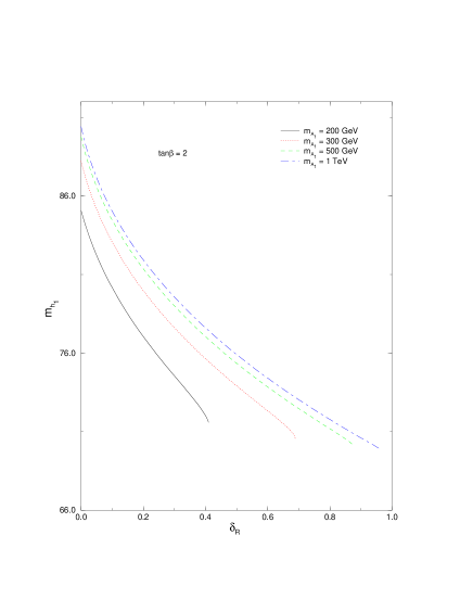
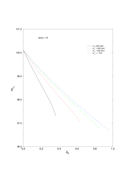
Figure 3: $m_{h_{1}}$ and $m_{h_{2}}$ as a function of $\delta_{R}$ for $m_{A_{1}}=200,300,500,1000$ GeV and $m_{A_{2}}=100$ GeV. The input parameters for the loop contributions to the difference between the CP-even and CP-odd mass matrices are $m_{Q}=500$ GeV, $m_{U}=m_{D}=300$ GeV, $A=200$ GeV, and $\mu_{I}=(200,0)$. In the plots on the left, $\tan\beta=2$; $\tan\beta=10$ for the plots on the right.

Conversely, in fig. 4 we present the variation of $m_{h_{1}}$ with respect to $m_{A_{2}}$ for $\delta_{R}=0,0.2,0.5,0.8$, having fixed $m_{A_{1}}=1$ TeV, and for two values of $\tan\beta=2,10$. For each value of $\delta_{R}$ there is a maximum allowed value of $m_{A_{2}}$. Recall that $A_{2}$ is a sneutrino component when $\delta_{R}=0$. As $m_{A_{2}}\rightarrow 0$, so does $m_{h_{1}}$ because the lightest CP-even Higgs is the mode that becomes $\tilde{\nu}_{R}$ when $\delta_{R}=0$. As $m_{A_{2}}$ increases, the mode “that would be the MSSM $h$ if $\delta_{R}=0$” becomes the lightest Higgs and the plot flattens out. In the plot $m_{h_{1}}$ does not become exactly zero for $\delta_{R}=0$, $m_{A_{2}}=0$ due to one-loop corrections proportional to $\lambda^{\prime 2}$ from the squark-quark sector.

     

Figure 4: $m_{h_{1}}$ as a function of $m_{A_{2}}$ for $\delta_{R}=0,0.2,0.5,0.8$ and $m_{A_{1}}=1$ TeV. The input parameters for the CP-even — CP-odd Higgs mass difference are $m_{Q}=500$ GeV, $m_{U}=m_{D}=300$ GeV, $A=200$ GeV, and $\mu_{I}=(200,0)$. $\tan\beta=2$ on the left, and $\tan\beta=10$ on the right.

As mentioned above, the loop corrections induced by values $\lambda^{\prime}\sim 1$ are similar to those induced by the top Yukawa for the Higgs which couples to the up-type sector. The other $R_{p}$-violating coupling we have introduced in the calculation $\mu_{1}$ is always constrained by the neutrino mass to be sufficiently small that its contributions are negligible.

Including $R$-parity violation in the Higgs sector can be understood as having two effects on Higgs production and decay. It mixes the “Higgses” with the “sneutrino”, and allows new decay modes for the Higgs/sneutrino decay products. There is of course no distinction between a Higgs and a sneutrino in the presence of $R$-parity violating couplings; by “sneutrino” we here mean the CP-even and -odd mass eigenstates that become the sneutrino in the $\delta_{R}\rightarrow 0$ limit, and the “Higgs” is the CP-even mass eigenstate that would be the Higgs in the same limit. We define $A_{2}$ to be the CP-odd scalar that becomes the $\tilde{\nu}_{I}$ as $\delta_{R}\rightarrow 0$. Mixing the Higgs with the sneutrino means that the eigenstates $h_{i}$ can all be produced via $Z\rightarrow Zh_{i}$ and $Z\rightarrow h_{i}A_{j}$, where $i:1..3$ and $j:1..2$. All of the $h_{i}$ can decay to $b\bar{b}$, and to $\chi^{0}\nu$, $\chi^{+}\tau$ and $\chi\chi$ if these decay modes are kinematically accessible.

The neutralino can decay in the detector, via its production vertex (the neutralino becomes a neutrino and an off-shell Higgs, which can then decay to SM fermions). So unless $\delta_{R}$ is uninterestingly small, the $\chi^{0}\nu$ and $\chi^{0}\chi^{0}$ should be visible.

The new $R_{p}$ violating decay modes $h_{1}\rightarrow\chi^{+}\tau$ and $h_{1}\rightarrow\chi^{0}\nu$ have been previously discussed [34, 35]. We plot the branching ratio to $\chi^{0}\nu$ as a function of $\delta_{R}$ in figure (5). We assume in this plot that the decays to $\chi^{+}\tau$ and $\chi^{0}\chi^{0}$ are kinematically forbidden. As expected from equation (36), the decay rate increases with $\delta_{R}$. The decrease at large $\delta_{R}$ is a consequence of our parametrisation. $\delta_{R}$ is $\sin^{2}$ of the angle between the vectors $\vec{v}$ and $\vec{M}_{u}$; as the angle increases to $\pi/2$ for fixed $m_{A_{1}}$ and $m_{A_{2}}$, $|\vec{M}_{u}|$ decreases. So the $R_{p}$ violating mass term $|\vec{M}_{u}|\sqrt{\delta_{R}}$ decreases. For larger values of $\tan\beta$ the decay $h_{1}\rightarrow b\bar{b}$ is dominant.

     

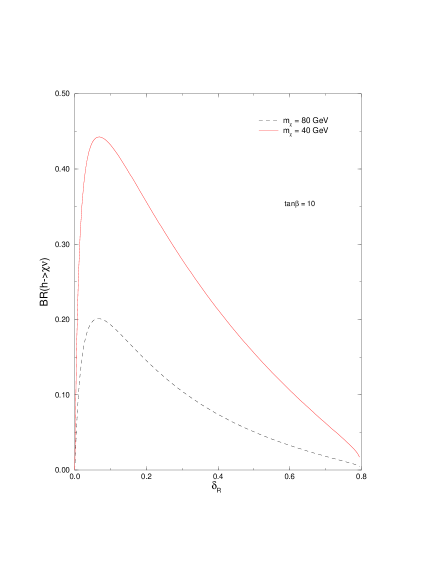
Figure 5: The branching ratio for $h_{1}\rightarrow\chi^{0}\nu$ as a function of $\delta_{R}$, for different values of $m_{\chi}$ and $\tan\beta$. We take $m_{A_{1}}=500$ GeV, $m_{A_{2}}=120$GeV , and the input parameters for the loops contributing to the CP-even—CP-odd Higgs mass difference are $A=0$, $\mu_{I}=(200,0)$, $m_{Q}=500$ GeV, $m_{U}=m_{D}=300$GeV. We take the total decay rate to be $\Gamma_{tot}$ $=\Gamma(h\rightarrow b\bar{b})$ $+\Gamma(h\rightarrow\chi^{0}\nu)$.

Suppose now that the neutralino is also heavier than $h_{1}$, so only the Standard Model decays are available to the Higgs. The $R_{p}$ violating couplings can still affect the production cross-section of the Higgs, and therefore the experimental lower limits on $m_{h}$.

The production cross-section for $Z\rightarrow Zh$ can be parametrised by $\xi^{2}=\sigma(Z\rightarrow Zh)/\sigma(Z\rightarrow Zh)_{SM}$. See, $e.g.$, [56] for experimental limits on $\xi^{2}$. In the MSSM, $\xi^{2}=\sin^{2}(\beta-\alpha)$. It can be very small in our $R_{p}$ violating model because it goes to zero as $\delta_{R}\rightarrow 0$ for the CP-even Higgs that becomes $\tilde{\nu}$ in this limit.

If $m_{A_{2}}$ is heavier than the CP-even Higgs which becomes $h$ of the MSSM in the $\delta_{R}\rightarrow 0$ limit, then the CP-even Higgs corresponding to $\tilde{\nu}_{R}$ in the same limit will be heavier than $m_{A_{2}}$ (see figure 3). In this case the $Z\rightarrow Zh_{1}$ vertex (equations 30 and 39) does not differ much from its MSSM value. We plot $\xi$ as a function of $\delta_{R}$ on the RHS of figure 6 for $m_{A_{2}}=100$ GeV. The present experimental lower limit on the Higgs mass for $\xi\sim.8$ is a few GeV below the $\xi=1$ limit of 95.2 GeV [56].

     

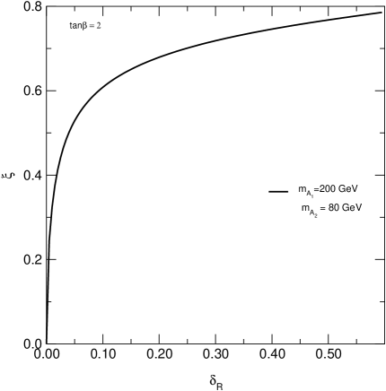
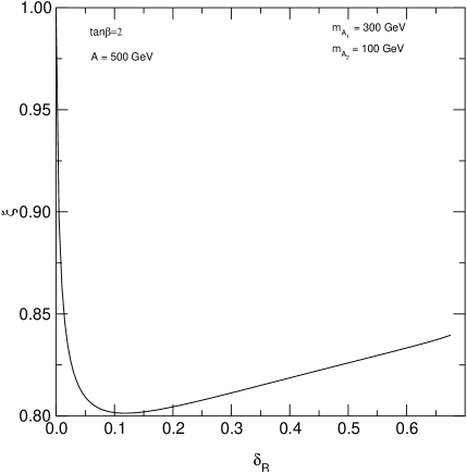
Figure 6: The ratio $\xi$ as a function of $\delta_{R}$, where $\xi=g_{ZZh}/g_{ZZh}^{SM}$ is the ratio of the $ZZh$ vertex its value in the SM. When the lightest CP-even scalar $h_{1}$ corresponds to the sneutrino in the $\delta_{R}\rightarrow 0$ limit, $\xi$ can be small and goes to zero with $\delta_{R}$. If $m_{A_{2}}($which becomes $m_{\tilde{\nu}}$ when $\delta_{R}=0$) is large, $\xi$ is near its MSSM value.

Alternatively, if $m_{A_{2}}$ is light , then $\xi^{2}$ can be very small. For instance on the LHS of figure 6, we plot $\xi$ for the CP-even Higgs which becomes part of the sneutrino when $\delta_{R}\rightarrow 0$. As expected, $\xi$ is very small for small $\delta_{R}$, because sneutrinos in the MSSM are pair-produced.

Decreasing the $ZZh$ vertex would decrease the experimental Higgs mass bound from this process; for $\xi\stackrel{{\scriptstyle<}}{{{}_{\sim}}}.3$, there is virtually no experimental lower limit [56]. However, $\Gamma(Z\rightarrow hA)$ increases as $\Gamma(Z\rightarrow hZ)$ decreases, so there should still be a bound on $m_{h}$. The experimental lower limit on $m_{h}$ from $Z\rightarrow hA$ is not trivial to determine, because the vertex and the two scalar masses are independent parameters. There are experimental limits in the MSSM [57], but in this case the vertex and $m_{h}$ determine $m_{A}$. There are also bounds on sneutrino masses from $Z\rightarrow\tilde{\nu}\tilde{\nu}^{*}$ [58] in models with trilinear $R_{p}$ violation, but these assume that the CP-even and CP-odd sneutrino components are degenerate. The experimental lower limits on the Higgs masses in this model are therefore unclear, but likely to be lower than in the MSSM.

7 Conclusions

We have described the $R$-parity violation induced by the additional soft mass terms in the scalar sector in terms of a basis-invariant quantity R (or $\delta_{R}$). This eliminates the ambiguity usually present in these models when a specific Lagrangian basis for the hypercharge $-1$ doublets is chosen. We have analysed the effects of the $R_{p}$-violating couplings on the CP-even and CP-odd scalar masses to one-loop in a basis-invariant way. We have also calculated the $R_{p}$ conserving and $R_{p}$ violating branching ratios of the lightest Higgs boson as a function of the basis-invariant quantity $\delta_{R}$. We have identified the regions of parameter space for which the decay modes of the Higgs boson are not those of the Standard Model Higgs. We have also calculated the production cross section as a function of $\delta_{R}$, and found that this can be strongly modified with respect to the $R_{p}$ conserving case when the lightest Higgs boson is mostly “sneutrino-like”. The LEP lower bound on the Higgs mass in this model can therefore be lower than in the MSSM.

Appendix A: $\langle\tilde{\nu}\rangle\neq 0$ basis

We take the potential $V$ to be the sum of equations (14) and (15). We define $v=\sqrt{v_{d}^{2}+v_{L}^{2}}$ $=\sqrt{v_{I}v^{I}}$, and

$$\tan\beta=\frac{\chi}{v}.$$ (45)

We write the stop and sbottom masses as

$$m_{\tilde{1},\tilde{2}}^{2}=\frac{1}{2}\left\{M_{L}^{2}+M_{R}^{2}\pm\sqrt{(M_{L}^{2}-M_{R}^{2})^{2}+2X^{2}}\right\}$$ (46)

where for the stops

$$M_{L}^{2}=m_{Q}^{2}+h_{t}^{2}\chi^{2}/2+(g^{2}-{1\over 3}g^{\prime 2})(v^{2}-\chi^{2})/8$$ (47)

$$M_{R}^{2}=m_{U}^{2}+h_{t}^{2}\chi^{2}/2+g^{\prime 2}(v^{2}-\chi^{2})/6$$ (48)

and

$$X_{t}^{2}=(A_{t}\chi+h_{t}\mu\cdot v)^{2}$$ (49)

For the sbottoms

$$M_{L}^{2}=m_{Q}^{2}+(\lambda\cdot v)^{2}/2-(g^{2}+{1\over 3}g^{\prime 2})(v^{2}-\chi^{2})/8$$ (50)

$$M_{R}^{2}=m_{D}^{2}+(\lambda\cdot v)^{2}/2-g^{\prime 2}(v^{2}-\chi^{2})/12$$ (51)

and

$$X_{b}^{2}=(A_{b}\cdot v+\lambda\cdot\mu\chi)^{2}~{}~{}~{}.$$ (52)

The one loop minimization conditions can be expressed in terms of the CP odd mass matrix $M_{ij}$ as in equations (22) and (23):

$$M_{uu}+\frac{M_{uI}v^{I}}{\chi}=0$$ (53)

$$M_{uI}+\frac{{\bf M}_{IJ}v^{J}}{\chi}=0$$ (54)

The CP-odd mass matrix is:

$$\left[\begin{array}[]{cc}M_{uu}&\left(\begin{array}[]{cc}M_{ud}&M_{uL}\end{array}\right)\\ \left(\begin{array}[]{c}M_{ud}\\ M_{uL}\end{array}\right)&\left(\begin{array}[]{cc}{\bf M}_{dd}&{\bf M}_{dL}\\ {\bf M}_{dL}&{\bf M}_{LL}\end{array}\right)\end{array}\right]$$ (55)

where the components are

$$M_{uu} = m_{u}^{2}-\frac{m_{Z}^{2}\cos 2\beta}{2}+\left\{\frac{3h_{t}^{2}}{32\pi^{2}}[f(m_{\tilde{t}_{1}})+f(m_{\tilde{t}_{2}})-2f(m_{t})]+(\lambda^{I}\mu_{I})^{2}D_{b}+A_{t}^{2}D_{t}\right\}$$ (56)

$$M_{uI} = B_{I}+\left\{(h_{t}A_{t}D_{t})\mu_{I}+(\mu^{J}\lambda_{J}D_{b})A^{b}_{I}\right\}$$ (57)

$${\bf M}_{IJ} = [m^{2}_{L}]_{IJ}+\frac{m_{Z}^{2}\cos 2\beta}{2}\;\delta_{IJ}$$ (58)

$$~{}~{}~{}~{}~{}+\left\{\frac{3}{32\pi^{2}}[f(m_{\tilde{b}_{1}})+f(m_{\tilde{b}_{2}})-2f(m_{b})]\lambda_{I}\lambda_{J}+h_{t}^{2}D_{t}\mu_{I}\mu_{J}+D_{b}A^{b}_{I}A^{b}_{J}\right\}\ .$$

We have defined

$$f(m)=2m^{2}\left(\log\frac{m^{2}}{Q^{2}}-1\right)\ ,$$ (59)

where $Q^{2}$ is the renormalisation scale in the $\overline{MS}$ scheme, and

$$D_{t} \equiv \frac{3}{32\pi^{2}}\frac{1}{\Delta_{t}}[f(m_{\tilde{t}_{1}})-f(m_{\tilde{t}_{2}})]\ ,$$ (60)

$$D_{b} \equiv \frac{3}{32\pi^{2}}\frac{1}{\Delta_{b}}[f(m_{\tilde{b}_{1}})-f(m_{\tilde{b}_{2}})]$$ (61)

with

$$\Delta_{t}=m^{2}_{\tilde{t}_{1}}-m^{2}_{\tilde{t}_{2}}\ ,\Delta_{b}=m^{2}_{\tilde{b}_{1}}-m^{2}_{\tilde{b}_{2}}\ .$$ (62)

The CP-even scalar mass matrix is:

$$M^{{}^{\prime}}_{uu} = M_{uu}+m_{Z}^{2}\sin^{2}\beta+\left\{\frac{3h_{t}^{4}}{16\pi^{2}}\chi^{2}\log\frac{m_{\tilde{t}_{1}}^{2}m_{\tilde{t}_{2}}^{2}}{m_{t}^{4}}\right.$$ (63)

$$\left.+\frac{3h_{t}^{2}}{16\pi^{2}}\frac{2A_{t}X_{t}\chi}{\Delta_{t}}\log\frac{m_{\tilde{t}_{1}}^{2}}{m_{\tilde{t}_{2}}^{2}}+A_{t}^{2}X^{2}_{t}g(m_{\tilde{t}_{1}},m_{\tilde{t}_{2}})+(\lambda_{I}\mu^{I})^{2}X^{2}_{b}g(m_{\tilde{b}_{1}},m_{\tilde{b}_{2}})\right\}$$

$$M^{{}^{\prime}}_{uJ} = M_{uJ}-m_{Z}^{2}\cos\beta\sin\beta\frac{v_{J}}{v}+\left\{\left[\frac{3}{16\pi^{2}}(v_{K}\lambda^{K})(\mu_{K}\lambda^{K})\frac{X_{b}}{\Delta_{b}}\log\frac{m_{\tilde{b}_{1}}^{2}}{m_{\tilde{b}_{2}}^{2}}\right]\lambda_{J}\right.$$ (64)

$$\left.+\frac{3}{16\pi^{2}}\left[\frac{\chi h_{t}^{3}X_{t}}{\Delta_{t}}\log\frac{m_{\tilde{t}_{1}}^{2}}{m_{\tilde{t}_{2}}^{2}}\right]\mu_{J}+\left[X^{2}_{b}(\lambda_{K}\mu^{K})g(m_{\tilde{b}_{1}},m_{\tilde{b}_{2}})\right]A^{b}_{J}+\left[X^{2}_{t}h_{t}A_{t}g(m_{\tilde{t}_{1}},m_{\tilde{t}_{2}})\right]\mu_{J}\right\}$$

$${\bf M}^{{}^{\prime}}_{IJ} = {\bf M}_{IJ}+m_{Z}^{2}\cos^{2}\beta\frac{v_{I}v_{J}}{v^{2}}+\left\{\left[\frac{3}{16\pi^{2}}(v_{K}\lambda^{K})^{2}\log\frac{m_{\tilde{b}_{1}}^{2}m_{\tilde{b}_{2}}^{2}}{m_{b}^{4}}\right]\lambda_{I}\lambda_{J}\right.$$ (65)

$$\left.+\left[\frac{3}{16\pi^{2}}(v_{K}\lambda^{K})\frac{X_{b}}{\Delta_{b}}\log\frac{m_{\tilde{b}_{1}}^{2}}{m_{\tilde{b}_{2}}^{2}}\right](\lambda_{I}A^{b}_{J}+\lambda_{J}A^{b}_{I})+\left[X^{2}_{b}g(m_{\tilde{b}_{1}},m_{\tilde{b}_{2}})\right]A^{b}_{I}A^{b}_{J}\right.$$

$$+\left.\left[X^{2}_{t}h_{t}^{2}g(m_{\tilde{t}_{1}},m_{\tilde{t}_{2}})\right]\mu_{I}\mu_{J}\right\}$$

where

$$g(m_{1},m_{2})=\frac{3}{16\pi^{2}}\frac{1}{(m_{1}^{2}-m_{2}^{2})^{2}}\left[2-\frac{m^{2}_{1}+m^{2}_{2}}{m^{2}_{1}-m^{2}_{2}}\log\frac{m_{1}^{2}}{m_{2}^{2}}\right]\ .$$ (66)

Appendix B: $\langle\tilde{\nu}\rangle=0$

This Appendix contains one-loop formulae for the minimisation conditions, the CP-odd mass matrix and the CP-even mass matrix, in the basis where the sneutrino vev $\langle\tilde{\nu}\rangle=v_{L}$ is zero at one loop.

We define the up-type Higgs vev to be $\chi/\sqrt{2}$, and the down-type vev to be $v/\sqrt{2}$, so

$$\tan\beta=\frac{\chi}{v}$$ (67)

and $X_{t}=A_{t}\chi+h_{t}\mu v$.

In this basis, we can safely neglect the loop corrections due to $h_{b}$ and the soft trilinear coupling $A^{b}_{d}\propto h_{b}$, since they are constrain to be small by the $b$-quark mass $m_{b}=-h_{b}v/\sqrt{2}\ll v$. If $m_{1}^{2}\equiv[{\bf m}_{L}^{2}]_{dd},m_{2}^{2}\equiv m_{u}^{2}$ and $m_{3}^{2}\equiv B_{d}$ are tree-level Higgs mass terms, $\mu\equiv\mu_{0}$ ($\epsilon\equiv\mu_{1}$) is the $R_{p}$ conserving (violating) superpotential mass, and $A^{\prime}\equiv A^{b}_{L}$, then the minimisation conditions are

$$m_{1}^{2} = -m_{3}^{2}\tan\beta-\frac{1}{2}m_{Z}^{2}\cos 2\beta+\delta m_{1}^{2}$$ (68)

$$m_{2}^{2} = -m_{3}^{2}\cot\beta+\frac{1}{2}m_{Z}^{2}\cos 2\beta+\delta m_{2}^{2}$$ (69)

$${[{\bf m}_{L}^{2}]}_{dL} = -B_{L}\tan\beta-h_{t}\epsilon D_{t}\frac{X_{t}}{v}-A^{\prime}\lambda^{\prime}\epsilon\tan\beta D_{b}$$ (70)

where

$$\delta m_{1}^{2} = -h_{t}\mu D_{t}\frac{X_{t}}{v}\ ,$$ (71)

$$\delta m_{2}^{2} = -\frac{3}{32\pi^{2}}h_{t}^{2}[f(m_{\tilde{t}_{1}})+f(m_{\tilde{t}_{2}})-2f(m_{t})]-A_{t}D_{t}\frac{X_{t}}{\chi}-\lambda^{\prime 2}\epsilon^{2}D_{b}\ .$$ (72)

We have defined $D_{t},D_{b}$ and $f(m)$ as in the previous appendix.

The CP-odd scalar mass matrix elements are

$$M_{uu} = -\cot\beta(m_{3}^{2}+h_{t}\mu A_{t}D_{t})$$ (73)

$$M_{ud} = m_{3}^{2}+h_{t}\mu A_{t}D_{t}$$ (74)

$$M_{uL} = B_{L}+h_{t}A_{t}\epsilon D_{t}+A^{\prime}\epsilon\lambda^{\prime}D_{b}$$ (75)

$${\bf M}_{dd} = -\tan\beta(m_{3}^{2}+h_{t}\mu A_{t}D_{t})$$ (76)

$${\bf M}_{dL} = [{\bf m}_{L}^{2}]_{dL}+h_{t}^{2}\mu\epsilon D_{t}$$ (77)

$${\bf M}_{LL} = m_{A_{1}}^{2}+m_{A_{2}}^{2}+(m_{3}^{2}+h_{t}\mu A_{t}D_{t})\frac{2}{\sin 2\beta}$$ (78)

with

$$m_{3}^{2} = -\frac{1}{2}\left\{(m_{A_{1}}^{2}+m_{A_{2}}^{2})\sin\beta\cos\beta+2h_{t}\mu A_{t}D_{t}\right\}$$

$$-\frac{\sin\beta\cos\beta}{2}\sqrt{(m_{A_{1}}^{2}-m_{A_{2}}^{2})^{2}-\frac{4}{\cos^{2}\beta}(B_{L}+h_{t}A_{t}\epsilon D_{t}+\lambda^{\prime}A^{\prime}\epsilon D_{b})^{2}}$$

The CP-even scalar mass matrix $M^{\prime}$ is:

$$M^{\prime}_{uu} = -\cot\beta(m_{3}^{2}+h_{t}\mu A_{t}D_{t})+m_{Z}^{2}\sin^{2}\beta+\lambda^{\prime 4}\epsilon^{4}\chi^{2}g(m_{\tilde{b}_{1}},m_{\tilde{b}_{2}})$$ (80)

$$+ \frac{3}{16\pi^{2}}\left[h_{t}^{4}\chi^{2}\log\frac{m_{\tilde{t}_{1}}^{2}m_{\tilde{t}_{2}}^{2}}{m_{t}^{4}}+\frac{2h_{t}^{2}A_{t}X_{t}\chi}{\Delta_{t}}\log\frac{m_{\tilde{t}_{1}}^{2}}{m_{\tilde{t}_{2}}^{2}}\right]+A_{t}^{2}X^{2}_{t}g(m_{\tilde{t}_{1}},m_{\tilde{t}_{2}})$$

$$M^{\prime}_{ud} = m_{3}^{2}-\frac{m_{Z}^{2}}{2}\sin 2\beta+h_{t}\mu A_{t}D_{t}+\frac{3h_{t}^{3}\mu X_{t}}{16\pi^{2}\Delta_{t}}\chi\log\frac{m_{\tilde{t}_{1}}^{2}}{m_{\tilde{t}_{2}}^{2}}+h_{t}\mu A_{t}X_{t}^{2}g(m_{\tilde{t}_{1}},m_{\tilde{t}_{2}})$$ (81)

$$M^{\prime}_{uL} = B_{L}+h_{t}A_{t}\epsilon D_{t}+\frac{3}{16\pi^{2}}h_{t}^{3}\frac{\epsilon X_{t}\chi}{\Delta_{t}}\log\frac{m_{\tilde{t}_{1}}^{2}}{m_{\tilde{t}_{2}}^{2}}+h_{t}A_{t}\epsilon X_{t}^{2}g(m_{\tilde{t}_{1}},m_{\tilde{t}_{2}})$$ (82)

$$+A^{\prime}\epsilon\lambda^{\prime}D_{b}+A^{\prime}\epsilon^{3}\lambda^{\prime 3}\chi^{2}g(m_{\tilde{b}_{1}},m_{\tilde{b}_{2}})$$

$${\bf M}^{\prime}_{dd} = -\tan\beta(m_{3}^{2}+h_{t}\mu A_{t}D_{t})+m_{Z}^{2}\cos^{2}\beta+h_{t}^{2}\mu^{2}X_{t}^{2}g(m_{\tilde{t}_{1}},m_{\tilde{t}_{2}})$$ (83)

$${\bf M}^{\prime}_{dL} = m_{dL}^{2}+h_{t}^{2}\mu\epsilon D_{t}+h_{t}^{2}X_{t}^{2}\mu\epsilon g(m_{\tilde{t}_{1}},m_{\tilde{t}_{2}})$$ (84)

$${\bf M}^{\prime}_{LL} = {\bf M}_{LL}+h_{t}^{2}\epsilon^{2}X_{t}^{2}g(m_{\tilde{t}_{1}},m_{\tilde{t}_{2}})+A^{\prime 2}\epsilon^{2}\lambda^{\prime 2}\chi^{2}g(m_{\tilde{b}_{1}},m_{\tilde{b}_{2}})$$ (85)

where $\Delta_{t}$ and $g(m_{1},m_{2})$ are as defined in the previous appendix.

Appendix C: Some equations

The normalisation factors for the basis-independent Higgs mixing angles, at tree level, are

$$\frac{u}{det[{\bf N^{\prime}}]}=-\frac{1}{\sqrt{(det\;{\bf N^{\prime}})^{2}+V^{{}^{\prime}2}}};$$ (86)

where N${}^{{}^{\prime}}=m_{h}^{2}$ I - M${}^{{}^{\prime}}$, and

$$\vec{V}^{\prime}={\bf N^{\prime}}\cdot\varepsilon\cdot\vec{M}^{{}^{\prime}}_{u}$$ (87)

For $h=h_{1},h_{2}$ or $h_{3}$,

$$\begin{array}[]{lcl}det\;{\bf N^{\prime}}&=&m_{h}^{4}-m_{h}^{2}(m_{Z}^{2}\cos^{2}\beta+m_{A_{1}}^{2}+m_{A_{2}}^{2})+\sin^{2}\beta m_{A_{1}}^{2}m_{A_{2}}^{2}+S(m_{h}^{2}-m_{Z}^{2})\\ &&+(m_{A_{1}}^{2}+m_{A_{2}}^{2})m_{Z}^{2}\cos^{2}\beta;\end{array}$$

and

$$\begin{array}[]{lcl}V^{{}^{\prime}2}&=&m_{h}^{4}(S^{2}\tan^{2}\beta/(1-\delta_{R})+2m_{Z}^{2}S\sin^{2}\beta+m_{Z}^{4}\cos^{2}\beta\sin^{2}\beta)\\ &&+m_{A_{1}}^{4}m_{A_{2}}^{4}\sin^{2}\beta\cos^{2}\beta+2m_{Z}^{2}\cos^{2}\beta\sin^{2}\beta(m_{A_{1}}^{2}m_{A_{2}}^{2}-m_{h}^{2}m_{Z}^{2})(m_{A_{1}}^{2}+m_{A_{2}}^{2}-S/\cos^{2}\beta)\\ &&+m_{Z}^{4}\cos^{2}\beta\sin^{2}\beta[(m_{A_{1}}^{2}+m_{A_{2}}^{2}-S)^{2}-2m_{A_{1}}^{2}m_{A_{2}}^{2}\sin^{2}\beta-S^{2}\tan^{4}\beta/(1-\delta_{R})]+\\ &&m_{Z}^{4}S^{2}\cos^{2}\beta\sin^{2}\beta\delta_{R}/(1-\delta_{R})-2m_{Z}^{2}\sin^{2}\beta m_{h}^{2}S^{2}\delta_{R}/(1-\delta_{R})\\ &&-2m_{h}^{2}m_{A_{1}}^{2}m_{A_{2}}^{2}\sin^{2}\beta(S+2m_{Z}^{2}\cos^{2}\beta)-2S^{2}m_{Z}^{4}\sin^{4}\beta\delta_{R}/(1-\delta_{R})\end{array}$$

For the CP-odd Higgses, the normalisation factor is

$$n=\frac{-1}{\sqrt{(det{\bf N})^{2}+V^{2}}}$$ (88)

where N = $m_{a}^{2}$ I - M, $\vec{V}=$ N $\cdot\varepsilon\cdot\vec{M}_{u}$, $a=$ either $A_{1}$ or $A_{2}$, and

$$det\;{\bf N}=m_{a}^{4}-m_{a}^{2}(m_{A_{1}}^{2}+m_{A_{2}}^{2}-S)+m_{A_{1}}^{2}m_{A_{2}}^{2}\sin^{2}\beta$$ (89)

and

$$V^{2}=m_{a}^{4}S^{2}\tan^{2}\beta/(1-\delta_{R})-2m_{a}^{2}m_{A_{1}}^{2}m_{A_{2}}^{2}S\sin^{2}\beta+m_{A_{1}}^{4}m_{A_{2}}^{4}\sin^{2}\beta\cos^{2}\beta$$ (90)

References

- [1] G.G.Ross. Grand Unified Theories. Benjamin-Cummings, Menlo Park, CA, 1985.
- [2] H.P. Nilles. Phys. Reports, 110:1, 1984.
- [3] H.E. Haber and G.L. Kane. Phys. Reports, 117:75, 1985.
- [4] R. Barbieri. Riv. Nuovo Cimento, 11:1, 1988.
- [5] L. E. Ibanez and G. G. Ross. Nucl. Phys., B368:3, 1992.
- [6] G.R. Farrar and P. Fayet. Nucl. Phys., B76:575, 1978.
- [7] A. Y. Smirnov and F. Vissani. Phys. Lett., B380:317, 1996.
- [8] L. Hall and M. Suzuki. Nucl. Phys., B231:419, 1984.
- [9] H. Dreiner. Perspectives on Supersymmetry. World Scientific, 1997; B.C. Allanach, A. Dedes, H.K. Dreiner Phys.Rev. D60 (1999) 075014.
- [10] G. Bhattacharyya. Nucl. Phys. Proc. Suppl., 52A:83, 1997. hep-ph/9608415.
- [11] R. Barbier et al.. Report of the GDR working group on R-parity violation. hep-ph/9810232.
- [12] H.-P. Nilles and N. Polonsky. Nucl. Phys., B484:33, 1997.
- [13] H. Dreiner, G.G. Ross, Nucl.Phys. B365 (1991) 597.
- [14] V. Barger G.F. Giudice and T.Han. Phys. Rev., D40:2987, 1989.
- [15] see, e.g B. Mukhopadhyaya, S. Roy, Phys.Rev. D60 (1999) 115012; A. Ghosal, Phys.Rev. D61 (2000) 075001, S.Y.Choi, E.J. Chun, S.Y. Kang, J.S. Lee, Phys.Rev.D60 (1999) 075002, and references therein.
- [16] J. Gunion and H. Haber. Nucl. Phys., B272:1, 1986.
- [17] J. Gunion, H. Haber, G. Kane, and S. Dawson. The Higgs Hunter’s Guide. Addison-Wesley, 1990.
- [18] H. Haber and R. Hempfling. Phys. Rev., D48:4280, 1993.
- [19] J.A. Casas, J.R. Espinosa, M. Quirós, and A. Riotto. Nucl. Phys., B436:3, 1995.
- [20] M. Carena, J.R. Espinosa, M. Quirós, and C. Wagner. Phys. Lett., B557:209, 1995.
- [21] D. Pierce, J. Bagger, K. Matchev, and R. Zhang. Nucl. Phys., B491:3, 1997.
- [22] Y. Okada, M. Yamaguchi, and T. Yanagida. Prog.Theor.Phys., 85:1, 1991.
- [23] A. Brignole. Phys. Lett., B277:313, 1992.
- [24] J. Ellis, G. Ridolfi, and F. Zwirner. Phys. Lett., B262:477, 1991.
- [25] J.R. Espinosa, M. Quirós, and F. Zwirner. Phys. Lett., B307:106, 1993.
- [26] P.H. Chankowski, S. Pokorski, and J. Rosiek. Phys. Lett., B274:191, 1992.
- [27] R. Hempfling and A. Hoang. Phys. Lett., B331:99, 1994.
- [28] H. Haber, R. Hempfling, and A. Hoang. Zeit. fur Phys., C75:539, 1997.
- [29] J.A. Casas, J.R. Espinosa, and H. Haber. Nucl. Phys., B526:3, 1998.
- [30] M. Carena, M. Quirós, and C.E.M. Wagner. Nucl. Phys., B461:407, 1996.
- [31] S. Heinemeyer, W. Hollik, and G. Weiglein. Phys. Lett., B455:179, 1999.
- [32] M. Carena, P.H. Chankowski, S. Pokorski, and C. Wagner. Phys. Lett., B441:205, 1998.
- [33] M. Carena and P. Zerwas. CERN yellow report, CERN-96-01, hep-ph/9602250.
- [34] F. de Campos, M.A. Garcia-Jareño, A.S. Joshipura, J. Rosiek and J.W.F. Valle. Nucl. Phys., B451:61, 1995.
- [35] M.A. Diaz, J.C. Romao, and J.W.F. Valle. Nucl. Phys., B524:23, 1998.
- [36] A. Akeroyd, M.A. Diaz, J. Ferrandis, M.A. Garcia-Jareño and J.W.F. Valle. Nucl. Phys., B529:3, 1998.
- [37] C.-H. Chang and T.-F. Feng. Eur. Phys. J. C12 (2000) 137.
- [38] C.-H. Chang and T.-F. Feng. hep-ph/9908295.
- [39] S. Davidson, T. Falk, and M. Losada. Phys. Lett. B463 (1999) 214.
-
[40]
G.F. Giudice.
Phys. Rev., D45:3177, 1992.
S. Myint. Phys. Lett., B287:325, 1992.
J.R. Espinosa, M. Quiros and F. Zwirner. Phys. Lett., B307:106, 1993.
A. Brignole, J.R. Espinosa, M. Quiros, F. Zwirner. Phys. Lett., B324:181, 1994.
M. Carena, M. Quiros, C. Wagner. Phys. Lett., B380:81 1996.
D. Delpine, J-M. Gerard, R. Gonzalez Felipe, J. Weyers. Phys. Lett., B386:183, 1996.
J.R. Espinosa. Nucl. Phys., B475:273, 1996.
M. Laine. Nucl. Phys., B481:43, 1996.
J. Cline, K. Kainulainen. Nucl. Phys., B482:73, 1996.
D. Bodeker, P.John, M. Laine, M.G. Schmidt. Nucl. Phys., B497:387, 1997.
B. de Carlos, J.R. Espinosa. Nucl. Phys., B503:24 1997.
G. Farrar, M. Losada. Phys. Lett., B406:60, 1997.
M Losada. Phys. Rev., D56:2893 1997, Nucl. Phys., B537:3 1999, Nucl. Phys. B569 (2000) 125.
M. Carena, M. Quiros, A. Riotto, I. Vilja and C. Wagner. Nucl. Phys., B503:387 1997.
J. Moreno, M. Quiros and M. Seco. Nucl. Phys., B526:489, 1998.
M. Laine and K. Rummukainen. Nucl. Phys., B535:423 1998, Nucl. Phys., B545:141 1998.
N. Rius and V. Sanz. Nucl.Phys B570 (2000) 155. - [41] T. Banks, Y. Grossman, E. Nardi, and Y. Nir. Phys. Rev., D52:5319, 1995.
- [42] S. Davidson and J. Ellis. Phys. Lett., B390:210, 1997.
- [43] S. Davidson and J. Ellis. Phys. Rev., D56:4182, 1997.
- [44] S. Davidson. Phys. Lett., B439:63, 1998.
- [45] M.Bisset, O.C. Kong, C. Macesanu, and L.H. Orr. Phys. Lett., B430:274,. hep–ph/9811498, 1998.
- [46] E. Nardi. Phys. Rev., D55:5772, 1997.
- [47] M. Nowakowski and A. Pilaftsis. Nucl. Phys., B461:19, 1996.
- [48] Y. Grossman and H. Haber. Phys. Rev. Lett., 78:3438, hep–ph/9909429, 1997.
- [49] Y. Grossman and H. Haber. Phys. Rev., D59:093008, hep–ph/9810536, 1999.
- [50] M. Hirsch, H.V. Klapdor-Kleingrothaus, and S.G. Kovalenko. Phys. Lett., B398:311, 1997.
- [51] G. Bhattacharyya, J. Ellis, and K. Sridhar. Mod.Phys.Lett., A10:1583, 1995.
- [52] K. Agashe and M. Graesser. Phys. Rev., D54:4445, 1996.
- [53] J. Erler, J. Feng, and N. Polonsky. Phys. Rev. Lett., 78:3063, 1997.
- [54] Y. Grossman, Z. Ligeti, and E. Nardi. Nucl. Phys., B465:369, 1996.
- [55] J. Ferrandis. Phys. Rev., D60:095012, 1999.
- [56] ALEPH, DELPHI, L3, OPAL, and The LEP working group for Higgs boson searches. In Int. Europhysics Conference on High Energy Physics, Tampere, Finland, July 1999.
- [57] The ALEPH Collaboration. Phys. Lett., B440:419, 1998.
- [58] ALEPH Collaboration. CERN-EP-99-093.