UMN–TH–1824/99

TPI–MINN–99/49

hep-ph/9911307

November 1999

Introduction to Supersymmetry:
Astrophysical and Phenomenological Constraints

Keith A. Olive

Theoretical Physics Institute,
School of Physics and Astronomy,
University of Minnesota,
Minneapolis, MN 55455, USA
Abstract

These lectures contain an introduction to supersymmetric theories and the minimal supersymmetric standard model. Phenomenological and cosmological consequences of supersymmetry are also discussed.

1 Introduction

It is often called the last great symmetry of nature. Rarely has so much effort, both theoretical and experimental, been spent to understand and discover a symmetry of nature, which up to the present time lacks concrete evidence. Hopefully, in these lectures, where I will give a pedagogical description of supersymmetric theories, it will become clear why there is so much excitement concerning supersymmetry’s role in nature.

After some preliminary background on the standard electroweak model, and some motivation for supersymmetry, I will introduce the notion of supersymmetric charges and the supersymmetric transformation laws. The second lecture will present the simplest supersymmetric model (the non-interacting massless Wess-Zumino model) and develop the properties of chiral superfields, auxiliary fields, the superpotential, gauge multiplets and interactions. The next two lectures focus on the minimal supersymmetric standard model (MSSM) and its constrained version which is motivated by supergravity. The last two lectures will look primarily at the cosmological and phenomenological consequences of supersymmetry.

1.1 Some Preliminaries

Why Supersymmetry? If for no other reason, it would be nice to understand the origin of the fundamental difference between the two classes of particles distinguished by their spin, fermions and bosons. If such a symmetry exists, one might expect that it is represented by an operator which relates the two classes of particles. For example,

$$Q|{\rm Boson}\rangle = |{\rm Fermion}\rangle$$

$$Q|{\rm Fermion}\rangle = |{\rm Boson}\rangle$$ (1)

As such, one could claim a raison d’etre for fundamental scalars in nature. Aside from the Higgs boson (which remains to be discovered), there are no fundamental scalars known to exist. A symmetry as potentially powerful as that in eq. (1) is reason enough for its study. However, without a connection to experiment, supersymmetry would remain a mathematical curiosity and a subject of a very theoretical nature as indeed it stood from its initial description in the early 1970’s [1, 2] until its incorporation into a realistic theory of physics at the electroweak scale.

One of the first break-throughs came with the realization that supersymmetry could help resolve the difficult problem of mass hierarchies [3], namely the stability of the electroweak scale with respect to radiative corrections. With precision experiments at the electroweak scale, it has also become apparent that grand unification is not possible in the absence of supersymmetry [4]. These issues will be discussed in more detail below.

Because one of our main goals is to discuss the MSSM, it will be useful to first describe some key features of the standard model if for no other reason than to establish the notation used below. The standard model is described by the SU(3)${}_{\rm c}\times$ SU(2)${}_{\rm L}\times$ U(1)_Y gauge group. For the most part, however, I will restrict the present discussion to the electroweak sector. The Lagrangian for the gauge sector of the theory can be written as

$${\cal L}_{G}=-\frac{1}{4}~{}G^{i}_{\mu\nu}G^{i\mu\nu}-{1\over 4}F_{\mu\nu}F^{\mu\nu}$$ (2)

where $G^{i}_{\mu\nu}\equiv\partial_{\mu}W^{i}_{\nu}-\partial_{\nu}W^{i}_{\mu}+g\epsilon^{ijk}W^{j}_{\mu}W^{k}_{\nu}$ is the field strength for the $SU(2)$ gauge boson $W^{i}_{\mu}$, and $F_{\mu\nu}\equiv\partial_{\mu}B_{\nu}-\partial_{\nu}B_{\mu}$ is the field strength for the $U(1)$ gauge boson $B_{\mu}$. The fermion kinetic terms are included in

$${\cal L}_{F}=-\sum_{f}i~{}~{}\left[\bar{f}_{L}\gamma^{\mu}D_{\mu}f_{L}+\bar{f}_{R}\gamma^{\mu}D_{\mu}f_{R}\right]$$ (3)

where the gauge covariant derivative is given by

$$D_{\mu}\equiv\partial_{\mu}-i~{}g~{}{\sigma_{i}\over 2}~{}W^{i}_{\mu}-i~{}g^{\prime}~{}{Y\over 2}~{}B_{\mu}$$ (4)

The $\sigma_{i}$ are the Pauli matrices (representations of SU(2)) and Y is the hypercharge. $g$ and $g^{\prime}$ are the SU(2)_L and U(1)_Y gauge couplings respectively.

Fermion mass terms are generated through the coupling of the left- and right-handed fermions to a scalar doublet Higgs boson $\phi$.

$${\cal L}_{Y}=-\sum_{f}\left[G_{f}\phi\bar{f}_{L}f_{R}\right]+h.c.$$ (5)

The Lagrangian for the Higgs field is

$${\cal L}_{\phi}=-|D_{\mu}\phi|^{2}-V(\phi)$$ (6)

where the (unknown) Higgs potential is commonly written as

$$V(\phi)=-\mu^{2}\phi^{\dagger}\phi+{\lambda}(\phi^{\dagger}\phi)^{2}$$ (7)

The vacuum state corresponds to a Higgs expectation value

$$\langle\phi\rangle=\langle\phi^{*}\rangle=\left(\matrix{0\cr{v}}\right)\qquad{\rm with}\qquad v^{2}={\mu^{2}\over 2\lambda}$$ (8)

The non-zero expectation value and hence the spontaneous breakdown of the electroweak gauge symmetry generates masses for the gauge bosons (through the Higgs kinetic term in (6) and fermions (through (5)). In a mass eigenstate basis, the charged $W$-bosons ($W^{\pm}\equiv(W^{1}\pm iW^{2})/\sqrt{2})$ receive masses

$$M_{W}={1\over\sqrt{2}}gv$$ (9)

The neutral gauge bosons are defined by

$$Z_{\mu}={gW^{3}_{\mu}-g^{\prime}B_{\mu}\over\sqrt{g^{2}+g^{\prime 2}}}~{}\qquad A_{\mu}={g^{\prime}W^{3}_{\mu}+gB_{\mu}\over\sqrt{g^{2}+g^{\prime 2}}}$$ (10)

with masses

$$M_{Z}={1\over\sqrt{2}}\sqrt{g^{2}+g^{\prime 2}}~{}v=M_{W}/\cos\theta_{W}\qquad m_{\gamma}=0$$ (11)

where the weak mixing angle is defined by

$$\sin\theta_{W}=g^{\prime}/\sqrt{g^{2}+g^{\prime 2}}$$ (12)

Fermion masses are

$$m_{f}=G_{f}v$$ (13)

As one can see, there is a direct relationship between particle masses and the Higgs expectation value, $v$. Indeed, we know from (9) and (11) that $v\sim M_{W}\sim O(100)$ GeV. We can then pose the question, why is $M_{W}\ll M_{P}=1.2\times 10^{19}$ GeV or equivalently why is $G_{F}\gg G_{N}$?

1.2 The hierarchy problem

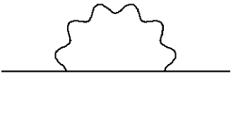
The mass hierarchy problem stems from the fact that masses, in particular scalar masses, are not stable to radiative corrections [3]. While fermion masses also receive radiative corrections from diagrams of the form in Figure 1, these are only logarithmically divergent (see for example [5]),

$$\delta m_{f}\simeq{3\alpha\over 4\pi}m_{f}\ln(\Lambda^{2}/m_{f}^{2})$$ (14)

$\Lambda$ is an ultraviolet cutoff, where we expect new physics to play an important role. As one can see, even for $\Lambda\sim M_{P}$, these corrections are small, $\delta m_{f}\mathrel{\raise 1.29167pt\hbox{$<$\kern-7.5pt\lower 4.30554pt\hbox{$\sim$}}}m_{f}$.

Figure 1: 1-loop correction to a fermion mass.

In contrast, scalar masses are quadratically divergent. 1–loop contributions to scalars masses, such as those shown in Figure 2 are readily computed

$$\delta m_{H}^{2}\simeq g_{f}^{2},g^{2},\lambda\int d^{4}k{1\over k^{2}}\sim O({\alpha\over 4\pi})\Lambda^{2}$$ (15)

due to contributions from fermion loops with coupling $g_{f}$, from gauge boson loops with coupling $g^{2}$, and from quartic scalar-couplings $\lambda$. From the relation (9) and the fact that the Higgs mass is related to the expectation value, $m_{H}^{2}=4v^{2}\lambda$, we expect $M_{W}\sim m_{H}$. However, if new physics enters in at the GUT or Planck scale so that $\Lambda\gg M_{W}$, the 1–loop corrections destroy the stability of the weak scale. That is,

$$\Lambda\gg M_{W}\rightarrow\delta m_{H}^{2}\gg m_{H}^{2}$$ (16)

Figure 2: 1-loop corrections to a scalar mass.

Of course, one can tune the bare mass $m_{H}$ so that it contains a large negative term which almost exactly cancels the 1–loop correction leaving a small electroweak scale mass². For a Planck scale correction, this cancellation must be accurate to 32 significant digits. Even so, the 2-loop corrections should be of order $\alpha^{2}\Lambda^{2}$ so these too must be accurately canceled. Although such a series of cancellations is technically feasible, there is hardly a sense of satisfaction that the hierarchy problem is under control.

An alternative and by far simpler solution to this problem exists if one postulates that there are new particles with similar masses and equal couplings to those responsible for the radiatively induced masses but with a difference (by a half unit) in spin. Then, because the contribution to $\delta m_{H}^{2}$ due to a fermion loop comes with a relative minus sign, the total contribution to the 1-loop corrected mass² is

$$\delta m_{H}^{2}\simeq O({\alpha\over 4\pi})(\Lambda^{2}+m_{B}^{2})-O({\alpha\over 4\pi})(\Lambda^{2}+m_{F}^{2})=O({\alpha\over 4\pi})(m^{2}_{B}-m^{2}_{F})$$ (17)

If in addition, the bosons and fermions all have the same masses, then the radiative corrections vanish identically. The stability of the hierarchy only requires that the weak scale is preserved so that we need only require that

$$|m^{2}_{B}-m^{2}_{F}|\mathrel{\raise 1.29167pt\hbox{$<$\kern-7.5pt\lower 4.30554pt\hbox{$\sim$}}}1~{}{\rm TeV}^{2}$$ (18)

As we will see in the lectures that follow, supersymmetry offers just the framework for including the necessary new particles and the absence of these dangerous radiative corrections [6].

Before we embark, I would like to call attention to some excellent additional resources on supersymmetry. These are the classic by Bagger and Wess on supersymmetry, [7], the book by Ross on Grand Unification [8] and two recent reviews by Martin [9] and Ellis [10].

1.3 Supersymmetric operators and transformations

Prior to the introduction of supersymmetry, operators were generally regarded as bosonic. That is, they were either scalar, vector, or tensor operators. The momentum operator, $P_{\mu}$, is a common example of a vector operator. However, the types of bosonic charges are greatly limited, as was shown by Coleman and Mandula [11]. Given a tensorial operator, $\Sigma_{\mu\nu}$, its diagonal matrix elements can be decomposed as

$$<a|\Sigma_{\mu\nu}|a>=\alpha p^{a}_{\mu}p^{a}_{\nu}+\beta g_{\mu\nu}$$ (19)

One can easily see that unless $\alpha=0$, 2 to 2 scattering process allow only forward scattering.

Operators of the form expressed in (1) however, are necessarily non-diagonal as they require a change between the initial and final state by at least a half unit of spin. Indeed, such operators, if they exist must be fermionic in nature and carry a spinor index $Q_{\alpha}$. There may in fact be several such operators, $Q_{\alpha}^{i}$ with $i=1,...,N$, (though for the most part we will restrict our attention to $N=1$ here). As a symmetry operator, $Q$ must commute with the Hamiltonian $H$, as must its anti-commutator. So we have

$$[Q^{i}_{\alpha},H]=0\qquad[\{Q^{i}_{\alpha},Q^{j}_{\beta}\},H]=0$$ (20)

By extending the Coleman-Mandula theorem [12], one can show that

$$\{Q^{i},Q^{j\dagger}\}\propto\delta^{ij}P_{\mu}+Z^{ij}$$ (21)

where $Z^{ij}$ is antisymmetric in the supersymmetry indices $\{i,j\}$. Thus, this so-called “central charge” vanishes for $N=1$. More precisely, we have in a Weyl basis

$$\{Q_{\alpha},{Q^{\dagger}}_{\dot{\beta}}\} = 2\sigma^{\mu}_{\alpha\dot{\beta}}P_{\mu}$$

$$\{Q_{\alpha},Q_{{\beta}}\}=\{Q^{\dagger}_{\dot{\alpha}},{Q^{\dagger}}_{\dot{\beta}}\} = 0$$

$$\ [Q_{\alpha},P_{\mu}]=[{Q^{\dagger}}_{\dot{\alpha}},P_{\mu}] = 0$$ (22)

Before setting up the formalism of the supersymmetric transformations, it will be useful to establish some notation for dealing with spinors in the Dirac and Weyl bases. The Lagrangian for a four-component Dirac fermion with mass $M$, can be written as

$${\cal L}_{D}=-i\overline{\Psi}_{D}\gamma^{\mu}\partial_{\mu}\Psi_{D}-M\overline{\Psi}_{D}\Psi_{D}$$ (23)

where

$$\gamma_{\mu}=\pmatrix{0&\sigma_{\mu}\cr{\overline{\sigma}}_{\mu}&0\cr}\qquad\qquad\gamma_{5}=\pmatrix{-1&0\cr 0&1\cr}$$ (24)

and $\sigma_{\mu}=(1,\sigma_{i})$, ${\overline{\sigma}}_{\mu}=(1,-\sigma_{i})$, $\sigma_{i}$ are the ordinary $2\times 2$ Pauli matrices. I am taking the Minkowski signature to be $(-,+,+,+)$. We can write the Dirac spinor $\Psi_{D}$ in terms of 2 two-component Weyl spinors

$$\Psi_{D}=\pmatrix{\xi_{\alpha}\cr{\chi^{\dagger\dot{\alpha}}}\cr}\qquad\qquad\overline{\Psi}_{D}=\pmatrix{\chi^{\alpha}&{\xi^{\dagger}}_{\dot{\alpha}}\cr}$$ (25)

Note that the spinor indices ($\alpha,\dot{\alpha}$) are raised and lowered by $\epsilon_{ij}$ where $\{ij\}$ can be either both dotted or both undotted indices. $\epsilon$ is totally antisymmetric and $\epsilon_{ij}=-\epsilon^{ij}$ with $\epsilon^{12}=1$. It is also useful to define projection operators, $P_{L}$ and $P_{R}$ with

$$P_{L}\Psi_{D}={(1-\gamma_{5})\over 2}\Psi_{D}=\pmatrix{1&0\cr 0&0\cr}\Psi_{D}=\pmatrix{\xi_{\alpha}\cr 0\cr}$$ (26)

with a similar expression for $P_{R}$. In this way we can interpret $\xi_{\alpha}$ as a left-handed Weyl spinor and $\chi^{\dagger\dot{\alpha}}$ as a right-handed Weyl spinor. The Dirac Lagrangian (23) can now be written in terms of the two-component Weyl spinors as

$${\cal L}_{D}=-i\xi^{\dagger}\overline{\sigma}^{\mu}\partial_{\mu}\xi-i\chi^{\dagger}\overline{\sigma}^{\mu}\partial_{\mu}\chi-M(\xi\chi+\xi^{\dagger}\chi^{\dagger})$$ (27)

having used the identity, $-\chi\sigma^{\mu}\xi^{\dagger}=\xi^{\dagger}\overline{\sigma}^{\mu}\chi$.

Instead, it is sometimes convenient to consider a four-component Majorana spinor. This can be done rather easily from the above conventions and taking $\xi=\chi$, so that

$$\Psi_{M}=\pmatrix{\xi_{\alpha}\cr{\xi^{\dagger\dot{\alpha}}}\cr}\qquad\qquad\overline{\Psi}_{M}=\pmatrix{\xi^{\alpha}&{\xi^{\dagger}}_{\dot{\alpha}}\cr}$$ (28)

and the Lagrangian can be written as

$${\cal L}_{M} = -{i\over 2}\overline{\Psi}_{M}\gamma^{\mu}\partial_{\mu}\Psi_{M}-{1\over 2}M\overline{\Psi}_{M}\Psi_{M}$$ (29)

$$= -i\xi^{\dagger}\overline{\sigma}^{\mu}\partial_{\mu}\xi-{1\over 2}M(\xi\xi+\xi^{\dagger}\xi^{\dagger})$$

The massless representations for supersymmetry are now easily constructed. Let us consider here $N=1$ supersymmetry, i.e., a single supercharge $Q_{\alpha}$. For the massless case, we can choose the momentum to be of the form $P_{\mu}={1\over 4}(-1,0,0,1)$. As can be readily found from the anticommutation relations (22), the only non-vanishing anticommutation relation is $\{Q_{1},{Q^{\dagger}}_{\dot{1}}\}=1$. Consider then a state of given spin, $|\lambda\rangle$ such that ${Q^{\dagger}}_{\dot{1}}|\lambda\rangle=0$. (If it is not 0, then due to the anticommutation relations, acting on it again with ${Q^{\dagger}}_{\dot{1}}$ will vanish.) From the state $|\lambda\rangle$, it is possible to construct only one other nonvanishing state, namely $Q_{1}|\lambda\rangle$ - the action of any of the other components of $Q_{\alpha}$ will vanish as well. Thus, if the state $|\lambda\rangle$ is a scalar, then the state $Q_{1}|\lambda\rangle$ will be a fermion of spin 1/2. This (super)multiplet will be called a chiral multiplet. If $|\lambda\rangle$ is spin 1/2, then $Q_{1}|\lambda\rangle$ is a vector of spin 1, and we have a vector multiplet. In the absence of gravity (supergravity), these are the only two types of multiplets of interest.

For $N>1$, one can proceed in an analogous way. For example, with $N=2$, we begin with two supercharges $Q^{1},Q^{2}$. Starting with a state $|\lambda\rangle$, we can now obtain the following: $Q^{1}_{1}|\lambda\rangle$, $Q^{2}_{1}|\lambda\rangle,Q^{1}_{1}Q^{2}_{1}|\lambda\rangle$. In this case, starting with a complex scalar, one obtains two fermion states, and one vector, hence the vector (or gauge) multiplet. One could also start with a fermion state (say left-handed) and obtain two complex scalars, and a right-handed fermion. This matter multiplet however, is clearly not chiral and is not suitable for phenomenology. This problem persists for all supersymmetric theories with $N>1$, hence the predominant interest in $N=1$ supersymmetry.

Before we go too much further, it will be useful to make a brief connection with the standard model. We can write all of the standard model fermions in a two-component Weyl basis. The standard model fermions are therefore

$$Q_{i} = \pmatrix{u\cr d\cr}_{L},\qquad\pmatrix{c\cr s\cr}_{L},\qquad\pmatrix{t\cr b\cr}_{L}$$

$$u^{c}_{i} = ~{}~{}u^{c}_{L},\qquad\qquad c^{c}_{L},\qquad\qquad t^{c}_{L}$$

$$d^{c}_{i} = ~{}~{}d^{c}_{L},\qquad\qquad s^{c}_{L},\qquad\qquad b^{c}_{L}$$

$$L_{i} = \pmatrix{\nu_{e}\cr e\cr}_{L},\qquad\pmatrix{\nu_{\mu}\cr\mu\cr}_{L},\qquad\pmatrix{\nu_{\tau}\cr\tau\cr}_{L}$$

$$e^{c}_{i} = ~{}~{}e^{c}_{L},\qquad\qquad\mu^{c}_{L},\qquad\qquad\tau^{c}_{L}$$ (30)

Note that the fields above are all left-handed. Color indices have been suppressed. From (29), we see that we would write the fermion kinetic terms as

$${\cal L}_{kin}=-iQ_{i}^{\dagger}\overline{\sigma}^{\mu}\partial_{\mu}Q_{i}-iu_{i}^{c\dagger}\overline{\sigma}^{\mu}\partial_{\mu}u^{c}_{i}-\cdots$$ (31)

As indicated above and taking the electron as an example, we can form a Dirac spinor

$$\Psi_{e}=\pmatrix{e_{L}\cr e^{c\dagger}_{L}\cr}=\pmatrix{e_{L}\cr e_{R}\cr}$$ (32)

A typical Dirac mass term now becomes

$$\overline{\Psi}_{e}\Psi_{e}=e^{c}_{L}e_{L}+e_{L}^{\dagger}{e^{c}_{L}}^{\dagger}=e_{R}^{\dagger}e_{L}+e_{L}^{\dagger}e_{R}$$ (33)

As we introduce supersymmetry, the field content of the standard model will necessarily be extended. All of the standard model matter fields listed above become members of chiral multiplets in $N=1$ supersymmetry. Thus, to each of the (Weyl) spinors, we assign a complex scalar superpartner. This will be described in more detail when we consider the MSSM.

To introduce the notion of a supersymmetric transformation, let us consider an infinitesimal spinor $\xi^{\alpha}$ with the properties that $\xi$ anticommutes with itself and the supercharge $Q$, but commutes with the momentum operator

$$\{\xi^{\alpha},\xi^{\beta}\}=\{\xi^{\alpha},Q_{\beta}\}=[P_{\mu},\xi^{\alpha}]=0$$ (34)

It then follows that since both $\xi$ and $Q$ commute with $P_{\mu}$, the combination $\xi Q$ also commutes with $P_{\mu}$ or

$$[P_{\mu},\xi Q]=[P_{\mu},\xi^{\dagger}Q^{\dagger}]=0$$ (35)

where by $\xi Q$ we mean $\xi Q=\xi^{\alpha}Q_{\alpha}=\epsilon_{\alpha\beta}\xi^{\alpha}Q^{\beta}=-\epsilon_{\alpha\beta}Q^{\beta}\xi^{\alpha}=\epsilon_{\beta\alpha}Q^{\beta}\xi^{\alpha}=Q\xi$. Similarly, $\xi^{\dagger}Q^{\dagger}=\xi^{\dagger}_{\dot{\alpha}}{Q^{\dagger}}^{\dot{\alpha}}$. Also note that $\xi^{\alpha}Q_{\alpha}=-\xi_{\alpha}Q^{\alpha}$. Finally, we can compute the commutator of $\xi Q$ and $\xi^{\dagger}Q^{\dagger}$,

$$[\xi Q,\xi^{\dagger}Q^{\dagger}] = \xi Q\xi^{\dagger}Q^{\dagger}-\xi^{\dagger}Q^{\dagger}\xi Q=\xi^{\alpha}Q_{\alpha}{\xi^{\dagger}}_{\dot{\beta}}{Q^{\dagger}}^{\dot{\beta}}-\xi^{\dagger}_{\dot{\beta}}{Q^{\dagger}}^{\dot{\beta}}\xi^{\alpha}Q_{\alpha}$$ (36)

$$= \xi^{\alpha}Q_{\alpha}{Q^{\dagger}}_{\dot{\beta}}\xi^{\dagger{\dot{\beta}}}-\xi^{\dagger{\dot{\beta}}}{Q^{\dagger}}_{\dot{\beta}}Q_{\alpha}\xi^{\alpha}$$

$$= 2\xi^{\alpha}\sigma_{\alpha{\dot{\beta}}}^{\mu}\xi^{\dagger{\dot{\beta}}}P_{\mu}-\xi^{\alpha}{Q^{\dagger}}_{\dot{\beta}}Q_{\alpha}\xi^{\dagger{\dot{\beta}}}-\xi^{\dagger{\dot{\beta}}}{Q^{\dagger}}_{\dot{\beta}}Q_{\alpha}\xi^{\alpha}$$

$$= 2\xi\sigma^{\mu}\xi^{\dagger}P_{\mu}$$

We next consider the transformation property of a scalar field, $\phi$, under the infinitesimal $\xi$

$$\delta_{\xi}\phi=(\xi^{\alpha}Q_{\alpha}+{\xi^{\dagger}}_{\dot{\beta}}{Q^{\dagger}}^{\dot{\beta}})\phi$$ (37)

As described above, we can pick a basis so that ${Q^{\dagger}}^{\dot{\beta}}\phi=0$. Let call the spin 1/2 fermion $Q_{\alpha}\phi=\sqrt{2}\psi_{\alpha}$, so

$$\delta_{\xi}\phi=\xi^{\alpha}Q_{\alpha}\phi=\sqrt{2}\xi^{\alpha}\psi_{\alpha}$$ (38)

To further specify the supersymmetry transformation, we must define the action of $Q$ and $Q^{\dagger}$ on $\psi$. Again, viewing $Q$ as a “raising” operator, we will write $Q_{\alpha}\psi_{\gamma}=-\sqrt{2}\epsilon_{\alpha\gamma}F$ and ${Q^{\dagger}}^{\dot{\beta}}\psi_{\gamma}=-\sqrt{2}i{\sigma^{\mu}_{\gamma}}^{\dot{\beta}}\partial_{\mu}\phi$, where $F$, as we will see, is an auxiliary field to be determined later. Even though we had earlier argued that $Q$ acting on the spin 1/2 component of the chiral multiplet should vanish, we must keep it here, though as we will see, it does not correspond to a physical degree of freedom. To understand the action of ${Q^{\dagger}}$, we know that it must be related to the scalar $\phi$, and on dimensional grounds (${Q^{\dagger}}\lambda$ is of mass dimension 3/2) it must be proportional to $P_{\mu}\phi$. Then

$$\delta_{\xi}\psi_{\gamma} = (\xi^{\alpha}Q_{\alpha}+{\xi^{\dagger}}_{\dot{\beta}}{Q^{\dagger}}^{\dot{\beta}})\psi_{\gamma}$$ (39)

$$= -\sqrt{2}\xi^{\alpha}\epsilon_{\alpha\gamma}F+\sqrt{2}i\sigma_{\gamma{\dot{\beta}}}^{\mu}\xi^{\dagger{\dot{\beta}}}\partial_{\mu}\phi$$

$$= \sqrt{2}\xi_{\gamma}F+\sqrt{2}i(\sigma^{\mu}\xi^{\dagger})_{\gamma}\partial_{\mu}\phi$$

Given these definitions, let consider the successive action of two supersymmetry transformations $\delta_{\xi}$ and $\delta_{\eta}$.

$$\delta_{\eta}\delta_{\xi}\phi = \sqrt{2}\delta_{\eta}(\xi^{\alpha}\psi_{\alpha})$$ (40)

$$= \sqrt{2}\bigl{[}-\sqrt{2}\xi^{\alpha}\eta^{\gamma}\epsilon_{\gamma\alpha}F+\sqrt{2}i\xi^{\alpha}\sigma_{\alpha{\dot{\beta}}}^{\mu}\eta^{\dagger{\dot{\beta}}}\partial_{\mu}\phi\bigr{]}$$

If we take the difference $(\delta_{\eta}\delta_{\xi}-\delta_{\xi}\delta_{\eta})\phi$, we see that the first term in (40) cancels if we write $\xi^{\alpha}\eta^{\gamma}\epsilon_{\gamma\alpha}=-\xi^{\alpha}\eta_{\alpha}$ and note that $\xi^{\alpha}\eta_{\alpha}=\eta^{\alpha}\xi_{\alpha}$. Therefore the difference can be written as

$$(\delta_{\eta}\delta_{\xi}-\delta_{\xi}\delta_{\eta})\phi=2(\eta\sigma^{\mu}\xi^{\dagger}-\xi\sigma^{\mu}\eta^{\dagger})P_{\mu}\phi$$ (41)

In fact it is not difficult to show that (41) is a result of the general operator relation

$$\delta_{\eta}\delta_{\xi}-\delta_{\xi}\delta_{\eta}=2(\eta\sigma^{\mu}\xi^{\dagger}-\xi\sigma^{\mu}\eta^{\dagger})P_{\mu}$$ (42)

Knowing the general relation (42) and applying it to a fermion $\psi_{\gamma}$ will allow us to determine the transformation properties of the auxiliary field $F$. Starting with

$$\delta_{\eta}\delta_{\xi}\psi_{\gamma}=-\sqrt{2}\xi^{\alpha}\epsilon_{\alpha\gamma}\delta_{\eta}F+2i\sigma^{\mu}_{\gamma{\dot{\beta}}}\xi^{\dagger{\dot{\beta}}}\eta^{\alpha}\partial_{\mu}\psi_{\alpha}$$ (43)

we use the Fierz identity $\chi_{\gamma}\eta^{\alpha}\zeta_{\alpha}+\eta_{\gamma}\zeta^{\alpha}\chi_{\alpha}+\zeta_{\gamma}\chi^{\alpha}\eta_{\alpha}=0$, and making the substitutions, $\chi_{\gamma}=\sigma^{\mu}_{\gamma{\dot{\beta}}}\xi^{\dagger{\dot{\beta}}},\eta=\eta$, and $\zeta=\partial_{\mu}\psi$, we have

$$\delta_{\eta}\delta_{\xi}\psi_{\gamma}=-\sqrt{2}\xi^{\alpha}\epsilon_{\alpha\gamma}\delta_{\eta}F-2i\bigl{\{}\eta_{\gamma}\partial_{\mu}\psi^{\alpha}\sigma^{\mu}_{\alpha{\dot{\beta}}}\xi^{\dagger{\dot{\beta}}}+\partial_{\mu}\psi_{\gamma}{\sigma^{\mu\alpha}}_{{\dot{\beta}}}\ \xi^{\dagger{\dot{\beta}}}\eta_{\alpha}\bigr{\}}$$ (44)

Next we use the spinor identity, $\chi^{\alpha}\ \sigma^{\mu}_{\alpha{\dot{\beta}}}\ \xi^{\dagger{\dot{\beta}}}=-{\xi^{\dagger}}_{\dot{\beta}}\ \overline{\sigma}^{\mu{\dot{\beta}}\alpha}\ \chi_{\alpha}$ along with $\eta^{\gamma}\chi_{\gamma}=\chi^{\gamma}\eta_{\gamma}$ (from above) to get

$$\delta_{\eta}\delta_{\xi}\psi_{\gamma}=-\sqrt{2}\xi^{\alpha}\epsilon_{\alpha\gamma}\delta_{\eta}F+2i\bigl{\{}\eta_{\gamma}{\xi^{\dagger}}_{\dot{\beta}}\ \overline{\sigma}^{\mu{\dot{\beta}}\alpha}\partial_{\mu}\psi_{\alpha}-\eta^{\alpha}\sigma^{\mu}_{\alpha{\dot{\beta}}}\xi^{\dagger{\dot{\beta}}}\partial_{\mu}\psi_{\gamma}\bigr{\}}$$ (45)

It is not hard to see then that the difference of the double transformation becomes

$$(\delta_{\eta}\delta_{\xi}-\delta_{\xi}\delta_{\eta})\psi_{\gamma} = 2(\eta\sigma^{\mu}\xi^{\dagger}-\xi\sigma^{\mu}\eta^{\dagger})P_{\mu}\psi_{\gamma}$$ (46)

$$-2\bigl{[}\eta_{\gamma}(\xi^{\dagger}\overline{\sigma}^{\mu}P_{\mu}\psi)-\xi_{\gamma}(\eta^{\dagger}\overline{\sigma}^{\mu}P_{\mu}\psi)\bigr{]}$$

$$+\sqrt{2}\bigl{(}\xi_{\gamma}\delta_{\eta}F-\eta_{\gamma}\delta_{\xi}F\bigr{)}$$

Thus, the operator relation (42) will be satisfied only if

$$\delta_{\xi}F=-\sqrt{2}(\xi^{\dagger}\overline{\sigma}^{\mu}P_{\mu}\psi)$$ (47)

and we have the complete set of transformation rules for the chiral multiplet.

2 The Simplest Models

2.1 The massless non-interacting Wess-Zumino model

We begin by writing down the Lagrangian for a single chiral multiplet containing a complex scalar field and a Majorana fermion

$${\cal L} = -\partial_{\mu}\phi^{*}\partial^{\mu}\phi-i\psi^{\dagger}\overline{\sigma}^{\mu}\partial_{\mu}\psi$$ (48)

$$= -\partial_{\mu}\phi^{*}\partial^{\mu}\phi-{i\over 2}(\psi^{\dagger}\overline{\sigma}^{\mu}\partial_{\mu}\psi-\partial_{\mu}\psi^{\dagger}\overline{\sigma}^{\mu}\psi)$$

where the second line in (48) is obtained by a partial integration and is done to simplify the algebra below.

We must first check the invariance of the Lagrangian under the supersymmetry transformations discussed in the previous section.

$$\delta{\cal L} = -\sqrt{2}\xi\partial^{\mu}\psi\partial_{\mu}\phi^{*}-{i\over\sqrt{2}}\xi^{\dagger}F^{*}\overline{\sigma}^{\mu}\partial_{\mu}\psi-{1\over\sqrt{2}}\xi\sigma^{\nu}\overline{\sigma}^{\mu}\partial_{\mu}\psi\partial_{\nu}\phi^{*}$$ (49)

$$\qquad\qquad+{i\over\sqrt{2}}\xi^{\dagger}\partial_{\mu}F^{*}\overline{\sigma}^{\mu}\psi+{1\over\sqrt{2}}\xi\sigma^{\nu}\overline{\sigma}^{\mu}\psi\partial_{\mu}\partial_{\nu}\phi^{*}+h.c.$$

Now with the help of still one more identity, $(\sigma^{\mu}\overline{\sigma}^{\nu}+\sigma^{\nu}\overline{\sigma}^{\mu})^{\beta}_{\alpha}=-2\eta^{\mu\nu}\delta^{\beta}_{\alpha}$, we can expand the above expression

$$\delta{\cal L} = -\sqrt{2}\xi\partial^{\mu}\psi\partial_{\mu}\phi^{*}$$ (50)

$$+{1\over\sqrt{2}}\xi\sigma^{\nu}\overline{\sigma}^{\mu}\psi\partial_{\mu}\partial_{\nu}\phi^{*}+\sqrt{2}\xi\partial^{\mu}\psi\partial_{\mu}\phi^{*}+{1\over\sqrt{2}}\xi\sigma^{\mu}\overline{\sigma}^{\nu}\partial_{\mu}\psi\partial_{\nu}\phi^{*}$$

$$-{i\over\sqrt{2}}\xi^{\dagger}\bigl{(}F^{*}\overline{\sigma}^{\mu}\partial_{\mu}\psi-\partial_{\mu}F^{*}\overline{\sigma}^{\mu}\psi\bigr{)}+h.c.$$

Fortunately, we now have some cancellations. The first and third terms in (50) trivially cancel. Using the commutivity of the partial derivative and performing a simple integration by parts we see that the second and fourth terms also cancel. We left with (again after an integration by parts)

$$\delta{\cal L}=-i\sqrt{2}\xi^{\dagger}F^{*}\overline{\sigma}^{\mu}\partial_{\mu}\psi+h.c.$$ (51)

indicating the lack of invariance of the Lagrangian (48).

We can recover the invariance under the supersymmetry transformations by considering in addition to the Lagrangian (48) the following,

$${\cal L}_{aux}=F^{*}F$$ (52)

and its variation

$$\delta{\cal L}_{aux}=\delta F^{*}F+F^{*}\delta F$$ (53)

The variation of the auxiliary field, $F$, was determined in (47) and gives

$$\delta{\cal L}_{aux}=i\sqrt{2}\xi^{\dagger}F^{*}\overline{\sigma}^{\mu}\partial_{\mu}\psi+h.c.$$ (54)

and exactly cancels the piece left over in (51). Therefore the Lagrangian

$${\cal L}=-\partial_{\mu}\phi^{*}\partial^{\mu}\phi-i\psi^{\dagger}\overline{\sigma}^{\mu}\partial_{\mu}\psi+F^{*}F$$ (55)

is fully invariant under the set of supersymmetry transformations.

2.2 Interactions for Chiral Multiplets

Our next task is to include interactions for chiral multiplets which are also consistent with supersymmetry. We will therefore consider a set of chiral multiplets, $(\phi_{i},\psi_{i},F_{i})$ and a renormalizable Lagrangian, ${\cal L}_{int}$. Renormalizability limits the mass dimension of any term in the Lagrangian to be less than or equal to 4. Since the interaction Lagrangian must also be invariant under the supersymmetry transformations, we do not expect any terms which are cubic or quartic in the scalar fields $\phi_{i}$. Clearly no term can be linear in the fermion fields either. This leaves us with only the following possibilities

$${\cal L}_{int}={1\over 2}A^{ij}\psi_{i}\psi_{j}+B^{i}F_{i}+h.c.$$ (56)

where $A^{ij}$ is some linear function of the $\phi_{i}$ and ${\phi^{i}}^{*}$ and $B^{i}$ is some function which is at most quadratic in the scalars and their conjugates. Here, and in all that follows, it will be assumed that repeated indices such as $ii$ are summed. Furthermore, since $\psi_{i}\psi_{j}=\psi_{j}\psi_{i}$ (spinor indices are suppressed), the function $A^{ij}$ must be symmetric in $ij$. As we will see, the functions $A$ and $B$ will be related by insisting on the invariance of (56).

We begin therefore with the variation of ${\cal L}_{int}$

$$\delta{\cal L}_{int} = {1\over 2}{\partial A^{ij}\over\partial\phi_{k}}(\sqrt{2}\xi\psi_{k})(\psi_{i}\psi_{j})+{1\over 2}{\partial A^{ij}\over\partial{\phi^{k}}^{*}}(\sqrt{2}\xi^{\dagger}{\psi^{k}}^{\dagger})(\psi_{i}\psi_{j})$$ (57)

$$+{1\over 2}A^{ij}(\sqrt{2}\xi F_{i}+\sqrt{2}i\sigma^{\mu}\xi^{\dagger}\partial_{\mu}\phi_{i})\psi_{j}$$

$$+{1\over 2}A^{ij}\psi_{i}(\sqrt{2}\xi F_{j}+\sqrt{2}i\sigma^{\mu}\xi^{\dagger}\partial_{\mu}\phi_{j})$$

$$+{\partial B^{i}\over\partial\phi_{j}}(\sqrt{2}\xi\psi_{j})F_{i}+{\partial B^{i}\over\partial{\phi^{j}}^{*}}(\sqrt{2}\xi^{\dagger}{\psi^{j}}^{\dagger})F_{i}$$

$$+B^{i}\sqrt{2}i\xi^{\dagger}\overline{\sigma}^{\mu}\partial_{\mu}\psi_{i}+h.c.$$

where the supersymmetry transformations of the previous section have already been performed. The notation $(\psi_{i}\psi_{j})$ refers to $\psi_{i}^{\alpha}{\psi_{j}}_{\alpha}$ as clearly spinor indices have everywhere been suppressed. The Fierz identity $(\xi\psi_{k})(\psi_{i}\psi_{j})+(\xi\psi_{i})(\psi_{j}\psi_{k})+(\xi\psi_{j})(\psi_{k}\psi_{i})=0$ implies that the derivative of the function $A^{ij}$ with respect to $\phi_{k}$ (as in the first term of (57)) must be symmetric in ${ijk}$. Because there is no such identity for the second term with derivative with respect to ${\phi^{k}}^{*}$, this term must vanish. Therefore, the function $A^{ij}$ is a holomorphic function of the $\phi_{i}$ only. Given these constraints, we can write

$$A^{ij}=-M^{ij}-y^{ijk}\phi_{k}$$ (58)

where by (56) we interpret $M^{ij}$ as a symmetric fermion mass matrix, and $y^{ijk}$ as a set of (symmetric) Yukawa couplings. In fact, it will be convenient to write

$$A^{ij}=-{\partial^{2}W\over\partial\phi_{i}\partial\phi_{j}}$$ (59)

where

$$W={1\over 2}M^{ij}\phi_{i}\phi_{j}+{1\over 6}y^{ijk}\phi_{i}\phi_{j}\phi_{k}$$ (60)

and is called the superpotential.

Noting that the 2nd and 3rd lines of (57) are equal due to the symmetry of $A^{ij}$, we can rewrite the remaining terms as

$$\delta{\cal L}_{int} = A^{ij}\psi_{i}(\sqrt{2}\xi F_{j}+\sqrt{2}i\sigma^{\mu}\xi^{\dagger}\partial_{\mu}\phi_{j})$$ (61)

$$+{\partial B^{i}\over\partial\phi_{j}}(\sqrt{2}\xi\psi_{j})F_{i}+{\partial B^{i}\over\partial{\phi^{j}}^{*}}(\sqrt{2}\xi^{\dagger}{\psi^{j}}^{\dagger})F_{i}$$

$$-B^{i}\sqrt{2}i\partial_{\mu}\psi_{i}\sigma^{\mu}\xi^{\dagger}+h.c.$$

using in addition one of our previous spinor identities on the last line. Further noting that because of our definition of the superpotential in terms of $A^{ij}$, we can write $A^{ij}\partial_{\mu}\phi_{j}=-\partial_{\mu}(\partial W/\partial\phi_{i})$. Then the 2nd and last terms of (61) can be combined as a total derivative if

$$B^{i}={\partial W\over\partial\phi_{i}}$$ (62)

and thus is also related to the superpotential $W$. Then the 4th term proportional to $\partial B^{i}/\partial{\phi^{j}}^{*}$ is absent due to the holomorphic property of $W$, and the definition of $B$ (62) allows for a trivial cancellation of the 1st and 3rd terms in (61). Thus our interaction Lagrangian (56) is in fact supersymmetric with the imposed relationships between the functions $A^{ij},B^{i}$, and the superpotential $W$.

After all of this, what is the auxiliary field $F$? It has been designated as an “auxiliary” field, because it has no proper kinetic term in (55). It can therefore be removed via the equations of motion. Combining the Lagrangians (55) and (56) we see that the variation of the Lagrangian with respect to $F$ is

$${\delta{\cal L}\over\delta F}={F^{i}}^{*}+W^{i}$$ (63)

where we can now use the convenient notation that $W^{i}=\partial W/\partial\phi_{i}$, $W_{i}^{*}=\partial W/\partial{\phi^{i}}^{*}$, and $W^{ij}=\partial^{2}W/\partial\phi_{i}\partial\phi_{j}$, etc. The vanishing of (63) then implies that

$$F_{i}=-W_{i}^{*}$$ (64)

Putting everything together we have

$${\cal L} = -\partial_{\mu}\phi^{i*}\partial^{\mu}\phi_{i}-i\psi^{i\dagger}\overline{\sigma}^{\mu}\partial_{\mu}\psi_{i}$$ (65)

$$-{1\over 2}(W^{ij}\psi_{i}\psi_{j}+W_{ij}^{*}{\psi^{i}}^{\dagger}{\psi^{j}}^{\dagger})-W^{i}W_{i}^{*}$$

As one can see the last term plays the role of the scalar potential

$$V(\phi_{i},\phi^{i*})=W^{i}W_{i}^{*}$$ (66)

2.3 Gauge Multiplets

In principle, we should next determine the invariance of the Lagrangian including a vector or gauge multiplet. To repeat the above exercise performed for chiral multiplets, while necessary, is very tedious. Here, I will only list some of the more important ingredients.

Similar to the definition in (4), the gauge covariant derivative acting on scalars and chiral fermions is

$$D_{\mu}=\partial_{\mu}-igT\cdot A_{\mu}$$ (67)

where $T$ is the relevant representation of the gauge group. For SU(2), we have simply that $T^{i}=\sigma^{i}/2$. In the gaugino kinetic term, the covariant derivative becomes

$$(D_{\mu}\lambda)^{a}=\partial_{\mu}\lambda^{a}+gf^{abc}A^{b}\lambda^{c}$$ (68)

where the $f^{abc}$ are the (antisymmetric) structure constants of the gauge group under consideration ($[T^{a},T^{b}]=if^{abc}T^{c}$). Gauge invariance for a vector field, $A^{a}_{\mu}$, is manifest through a gauge transformation of the form

$$\delta_{gauge}A^{a}_{\mu}=-\partial_{\mu}\Lambda^{a}+gf^{abc}\Lambda^{b}A^{c}_{\mu}$$ (69)

where $\Lambda$ is an infinitesimal gauge transformation parameter. To this, we must add the gauge transformation of the spin 1/2 fermion partner, or gaugino, in the vector multiplet

$$\delta_{gauge}\lambda^{a}=gf^{abc}\Lambda^{b}\lambda^{c}$$ (70)

Given our experience with chiral multiplets, it is not too difficult to construct the supersymmetry transformations for the the vector multiplet. Starting with $A_{\mu}$, which is real, and taking $QA_{\mu}=0$, one finds that

$$\delta_{\xi}A^{a}_{\mu}=i\bigl{[}\xi^{\dagger}\overline{\sigma}_{\mu}\lambda^{a}-{\lambda^{a}}^{\dagger}\overline{\sigma}_{\mu}\xi\bigr{]}$$ (71)

Similarly, applying the supersymmetry transformation to $\lambda^{a}$, leads to a derivative of $A^{a}_{\mu}$ (to account for the mass dimension) which must be in the form of the field strength $F^{a}_{\mu\nu}$, and an auxiliary field, which is conventionally named $D^{a}$. Thus,

$$\delta_{\xi}\lambda^{a}={1\over{2}}\bigl{(}\sigma^{\mu}\overline{\sigma}^{\nu}\xi\bigr{)}F^{a}_{\mu\nu}+i\xi D^{a}$$ (72)

As before, we can determine the transformation properties of $D^{a}$ by applying successive supersymmetry transformations as in (42) with the substitution $\partial_{\mu}\to D_{\mu}$ using (67) above. The result is,

$$\delta_{\xi}D^{a}=\bigl{[}\xi^{\dagger}\overline{\sigma}^{\mu}D_{\mu}\lambda^{a}+D_{\mu}{\lambda^{a}}^{\dagger}\overline{\sigma}^{\mu}\xi\bigr{]}$$ (73)

Also in analogy with the chiral model, the simplest Lagrangian for the vector multiplet is

$${\cal L}_{gauge}=-{1\over 4}F^{a}_{\mu\nu}{F^{a}}^{\mu\nu}-i{\lambda^{a}}^{\dagger}\overline{\sigma}^{\mu}D_{\mu}\lambda^{a}+{1\over 2}D^{a}D^{a}$$ (74)

In (74), the gauge kinetic terms are given in general by $F^{a}_{\mu\nu}=\partial_{\mu}A^{a}_{\nu}-\partial_{\nu}A^{a}_{\mu}+gf^{abc}A^{b}_{\mu}A^{c}_{\nu}$.

If we have both chiral and gauge multiplets in the theory (as we must) then we must make simple modifications to the supersymmetry transformations discussed in the previous section and add new gauge invariant interactions between the chiral and gauge multiplets which also respect supersymmetry. To (39), we must only change $\partial_{\mu}\to D_{\mu}$ using (67). To (47), it will be necessary to add a term proportional to $(T^{a}\phi)\xi^{\dagger}{\lambda^{a}}^{\dagger}$ so that,

$$\delta_{\xi}F=\sqrt{2}i(\xi^{\dagger}\overline{\sigma}^{\mu}D_{\mu}\psi)+2ig(T^{a}\phi)\xi^{\dagger}{\lambda^{a}}^{\dagger}$$ (75)

The new interaction terms take the form

$${\cal L}_{int}=\sqrt{2}gi\left[(\phi^{*}T^{a}\psi)\lambda^{a}-\lambda^{\dagger a}(\psi^{\dagger}T^{a}\phi)\right]\\ +g(\phi^{*}T^{a}\phi)D^{a}$$

Furthermore, invariance under supersymmetry requires not only the additional term in (75), but also the condition

$$W^{i}(T^{a})_{i}^{j}\phi_{j}=0$$ (76)

Finally, we must eliminate the auxiliary field $D^{a}$ using the equations of motion which yield

$$D^{a}=-g(\phi^{*}T^{a}\phi)$$ (77)

Thus the “D-term” is also seen to be a part of the scalar potential which in full is now,

$$V(\phi,\phi^{*})=|F^{i}|^{2}+{1\over 2}|D^{a}|^{2}=|W^{i}|^{2}+{1\over 2}g^{2}(\phi^{*}T^{a}\phi)^{2}.$$ (78)

Notice a very important property of the scalar potential in supersymmetric theories: the potential is positive semi-definite, $V\geq 0$.

2.4 Interactions

The types of gauge invariant interactions allowed by supersymmetry are scattered throughout the pieces of the supersymmetric Lagrangian. Here, we will simply identify the origin of a particular interaction term, its coupling, and associated Feynmann diagram. In the diagrams below, the arrows denote the flow of chirality. Here, $\psi$ will represent an incoming fermion, and $\psi^{\dagger}$ an outgoing one. While there is no true chirality associated with the scalars, we can still make the association as the scalars are partnered with the fermions in a given supersymmetric multiplet. We will indicate $\phi$ with an incoming scalar state, and $\phi^{*}$ with an outgoing one.

Starting from the superpotential (60) and the Lagrangian (65), we can identify several interaction terms and their associated diagrams:

• a fermion mass insertion from $W^{ij}\psi_{i}\psi_{j}$

$\qquad\qquad\qquad M^{ij}\psi_{i}\psi_{j}\qquad$

• a scalar-fermion Yukawa coupling, also from $W^{ij}\psi_{i}\psi_{j}$

$\qquad\qquad\qquad y^{ijk}\phi_{k}\psi_{i}\psi_{j}\qquad$

• a scalar mass insertion from $|W^{i}|^{2}$

$\qquad\qquad\qquad M^{il}{M_{jl}}^{*}\phi_{i}{\phi^{j}}^{*}\qquad$

• a scalar cubic interaction from $|W^{i}|^{2}$ (plus its complex conjugate which is not shown)

$\qquad\qquad\qquad{M_{li}}^{*}y^{ljk}{\phi^{i}}^{*}\phi_{j}\phi_{k}\qquad$

• and finally a scalar quartic interaction from $|W^{i}|^{2}$

$\qquad\qquad~{}~{}{y^{ijn}}y_{kln}^{*}\phi_{i}\phi_{j}{\phi^{k}}^{*}{\phi^{l}}^{*}\qquad$

Next we must write down the interactions and associated diagrams for the gauge multiplets. The first two are standard gauge field interaction terms in any non-abelian gauge theory (so that $f^{abc}\neq 0$) and arise from the gauge kinetic term $F_{\mu\nu}^{2}$, the third is an interaction between the vector and its fermionic partner, and arises from the gaugino kinetic term $\lambda^{\dagger}\overline{\sigma}^{\mu}D_{\mu}\lambda$.

• The quartic gauge interaction from $F_{\mu\nu}^{2}$ (to be summed over the repeated gauge indices)

$\qquad~{}~{}~{}~{}g^{2}f^{abc}f^{ade}{A^{b}}^{\mu}{A^{c}}^{\nu}{A^{d}}_{\mu}{A^{e}}_{\nu}\qquad$

• The trilinear gauge interaction also from $F_{\mu\nu}^{2}$

$\qquad~{}~{}gf^{abc}{A^{b}}^{\mu}{A^{c}}^{\nu}(\partial_{\mu}{A^{a}}_{\nu}-\partial_{\nu}{A^{a}}_{\mu})\qquad$

• The gauge-gaugino interaction from $\lambda^{\dagger}\overline{\sigma}^{\mu}D_{\mu}\lambda$

$\qquad~{}~{}~{}~{}gf^{abc}{A^{b}}_{\mu}{\lambda^{a}}^{\dagger}\overline{\sigma}^{\mu}\lambda^{c}\qquad$

If our chiral multiplets are not gauge singlets, then we also have interaction terms between the vectors and the fermions and scalars of the chiral multiplet arising from the chiral kinetic terms. Recalling that the kinetic terms for the chiral multiplets must be expressed in terms of the gauge covariant derivative (67), we find the following interactions, from$|D_{\mu}\phi|^{2}$ and $\psi^{\dagger}\overline{\sigma}^{\mu}D_{\mu}\psi$,

• a quartic interaction interaction involving two gauge bosons and two scalars,

$\qquad\qquad~{}~{}g^{2}{A^{a}}^{\mu}{A^{b}}_{\mu}(T^{a}\phi)(\phi^{*}T^{b})\qquad$

• a cubic interaction involving one gauge boson and two scalars,

$\qquad\qquad~{}~{}g({A^{a}}^{\mu}(T^{a}\phi)\partial_{\mu}\phi^{*}+h.c.)\qquad$

• a cubic interaction involving one gauge boson and two fermions,

$\qquad\qquad~{}~{}g({A^{a}}_{\mu}\psi^{\dagger}\overline{\sigma}^{\mu}(T^{a}\psi)+h.c.)\qquad$

Finally, there will be two additional diagrams. One coming from the interaction term involving both the chiral and gauge multiplet, and one coming from $D^{2}$,

• a cubic interaction involving a gaugino, and a chiral scalar and fermion pair,

$\qquad~{}~{}g((\phi^{*}T^{a}\psi)\lambda^{a}+h.c.)\qquad$

• another quartic interaction interaction involving a gaugino, and a chiral scalar and fermion pair,

$\qquad\qquad~{}~{}g^{2}(\phi^{*}T^{a}\phi)^{2}\qquad$

2.5 Supersymmetry Breaking

The world, as we know it, is clearly not supersymmetric. Without much ado, it is clear from the diagrams above, that for every chiral fermion of mass $M$, we expect to have a scalar superpartner of equal mass. This is, however, not the case, and as such we must be able to incorporate some degree of supersymmetry breaking into the theory. At the same time, we would like to maintain the positive benefits of supersymmetry such as the resolution of the hierarchy problem.

To begin, we must be able to quantify what we mean by supersymmetry breaking. From the anti-commutation relations (22), we see that we can write an expression for the Hamiltonian or $P^{0}$ using the explicit forms of the Pauli matrices as

$$P^{0}={1\over 4}\sum_{\alpha=1}^{2}\{Q_{\alpha},Q_{\dot{\alpha}}^{\dagger}\}$$ (79)

A supersymmetric vacuum must be invariant under the supersymmetry transformations and therefore would require $Q|0\rangle=0$ and $Q^{\dagger}|0\rangle=0$ and therefore corresponds to $H=0$ and also $V=0$. Thus, the supersymmetric vacuum must have $|F|=|D|=0$. Conversely, if supersymmetry is spontaneously broken, the vacuum is not annihilated by the supersymmetry charge $Q$ so that $Q|0\rangle=\chi$ and $\langle\chi|Q|0\rangle=f_{\chi}^{2}$, where $\chi$ is a fermionic field associated with the breakdown of supersymmetry and in analogy with the breakdown of a global symmetry, is called the Goldstino. For $f_{\chi}\neq 0$, $\langle 0|H|0\rangle=V_{0}\neq 0$, and requires therefore either (or both) $|F|\neq 0$ or $|D|\neq 0$. Mechanisms for the spontaneous breaking of supersymmetry will be discussed in the next lecture.

It is also possible that to a certain degree, supersymmetry is explicitly broken in the Lagrangian. In order to preserve the hierarchy between the electroweak and GUT or Planck scales, it is necessary that the explicit breaking of supersymmetry be done softly, i.e., by the insertion of weak scale mass terms in the Lagrangian. This ensures that the theory remain free of quadratic divergences [13]. The possible forms for such terms are

$${\cal L}_{soft} = -{1\over 2}M^{a}_{\lambda}\lambda^{a}\lambda^{a}-{1\over 2}({m^{2}})^{i}_{j}\phi_{i}{\phi^{j}}^{*}$$ (80)

$$-{1\over 2}{(BM)}^{ij}\phi_{i}\phi_{j}-{1\over 6}{(Ay)}^{ijk}\phi_{i}\phi_{j}\phi_{k}+h.c.$$

where the $M^{a}_{\lambda}$ are gaugino masses, $m^{2}$ are soft scalar masses, $B$ is a bilinear mass term, and $A$ is a trilinear mass term. Masses for the gauge bosons are of course forbidden by gauge invariance and masses for chiral fermions are redundant as such terms are explicitly present in $M^{ij}$ already. The diagrams corresponding to these terms are

• a soft supersymmetry breaking gaugino mass insertion

$\qquad\qquad\qquad M^{a}_{\lambda}\lambda^{a}\lambda^{a}\qquad$

• a soft supersymmetry breaking scalar mass insertion

$\qquad\qquad\qquad({m^{2}})^{i}_{j}\phi_{i}{\phi^{j}}^{*}\qquad$

• a soft supersymmetry breaking bilinear mass insertion

$\qquad\qquad\qquad{(BM)}^{ij}\phi_{i}\phi_{j}\qquad$

• a soft supersymmetry breaking trilinear scalar interaction

$\qquad\qquad\qquad{(Ay)}^{ijk}\phi_{i}\phi_{j}\phi_{k}\qquad$

We are now finally in a position to put all of these pieces together and discuss realistic supersymmetric models.

3 The Minimal Supersymmetric Standard Model

To construct the supersymmetric standard model [14] we start with the complete set of chiral fermions in (30), and add a scalar superpartner to each Weyl fermion so that each of the fields in (30) represents a chiral multiplet. Similarly we must add a gaugino for each of the gauge bosons in the standard model making up the gauge multiplets. The minimal supersymmetric standard model (MSSM) [15] is defined by its minimal field content (which accounts for the known standard model fields) and minimal superpotential necessary to account for the known Yukawa mass terms. As such we define the MSSM by the superpotential

$$W=\epsilon_{ij}\bigl{[}y_{e}H_{1}^{j}L^{i}e^{c}+y_{d}H_{1}^{j}Q^{i}d^{c}+y_{u}H_{2}^{i}Q^{j}u^{c}\bigr{]}+W_{\mu}$$ (81)

where

$$W_{\mu}=\epsilon_{ij}\mu H_{1}^{i}H_{2}^{j}$$ (82)

In (81), the indices, $\{ij\}$, are SU(2)_L doublet indices. The Yukawa couplings, $y$, are all $3\times 3$ matrices in generation space. Note that there is no generation index for the Higgs multiplets. Color and generation indices have been suppressed in the above expression. There are two Higgs doublets in the MSSM. This is a necessary addition to the standard model which can be seen as arising from the holomorphic property of the superpotential. That is, there would be no way to account for all of the Yukawa terms for both up-type and down-type multiplets with a single Higgs doublet. To avoid a massless Higgs state, a mixing term $W_{\mu}$ must be added to the superpotential.

From the rules governing the interactions in supersymmetry discussed in the previous section, it is easy to see that the terms in (81) are easily identifiable as fermion masses if the Higgses obtain vacuum expectation values (vevs). For example, the first term will contain an interaction which we can write as

$$-{1\over 2}{\partial^{2}W\over\partial L\partial e^{c}}\bigl{(}\psi_{L}\psi_{e^{c}}+\psi_{L}^{\dagger}\psi_{e^{c}}^{\dagger}\bigr{)}$$ (83)

$$= -{1\over 2}y_{e}H^{0}_{1}\bigl{(}\ e{e^{c}}+e^{\dagger}{e^{c}}^{\dagger}\bigr{)}$$

where it is to be understood that in (83) that $H_{1}$ refers to the scalar component of the Higgs $H_{1}$ and $\psi_{L}$ and $\psi_{e^{c}}$ represents the fermionic component of the left-handed lepton doublet and right-handed singlet respectively. Gauge invariance requires that as defined in (81), $H_{1}$ has hypercharge $Y_{H_{1}}=-1$ (and $Y_{H_{2}}=+1$). Therefore if the two doublets obtain expectation values of the form

$$\langle H_{1}\rangle=\pmatrix{v_{1}\cr 0\cr}\qquad\langle H_{2}\rangle=\pmatrix{0\cr v_{2}\cr}$$ (84)

then (83) contains a term which corresponds to an electron mass term with

$$m_{e}=y_{e}v_{1}$$ (85)

Similar expressions are easily obtained for all of the other massive fermions in the standard model. Clearly as there is no $\nu^{c}$ state in the minimal model, neutrinos remain massless. Both Higgs doublets must obtain vacuum values and it is convenient to express their ratio as a parameter of the model,

$$\tan\beta={v_{2}\over v_{1}}$$ (86)

3.1 The Higgs sector

Of course if the vevs for $H_{1}$ and $H_{2}$ exist, they must be derivable from the scalar potential which in turn is derivable from the superpotential and any soft terms which are included. The part of the scalar potential which involves only the Higgs bosons is

$$V = |\mu|^{2}(H_{1}^{*}H_{1}+H_{2}^{*}H_{2})+{1\over 8}{g^{\prime}}^{2}(H_{2}^{*}H_{2}-H_{1}^{*}H_{1})^{2}$$ (87)

$$+{1\over 8}{g}^{2}\left(4|H_{1}^{*}H_{2}|^{2}-2(H_{1}^{*}H_{1})(H_{2}^{*}H_{2})+(H_{1}^{*}H_{1})^{2}+(H_{2}^{*}H_{2})^{2}\right)$$

$$+m_{1}^{2}H_{1}^{*}H_{1}+m_{2}^{2}H_{2}^{*}H_{2}+(B\mu\epsilon_{ij}H_{1}^{i}H_{2}^{j}+h.c.)$$

In (87), the first term is a so-called $F$-term, derived from $|(\partial W/\partial H_{1})|^{2}$ and $|(\partial W/\partial H_{2})|^{2}$ setting all sfermion vevs equal to 0. The next two terms are $D$-terms, the first a U(1)-$D$-term, recalling that the hypercharges for the Higgses are $Y_{H_{1}}=-1$ and $Y_{H_{2}}=1$, and the second is an SU(2)-$D$-term, taking $T^{a}=\sigma^{a}/2$ where $\sigma^{a}$ are the three Pauli matrices. Finally, the last three terms are soft supersymmetry breaking masses $m_{1}$ and $m_{2}$, and the bilinear term $B\mu$. The Higgs doublets can be written as

$$\langle H_{1}\rangle=\pmatrix{H_{1}^{0}\cr H_{1}^{-}\cr}\qquad\langle H_{2}\rangle=\pmatrix{H_{2}^{+}\cr H_{2}^{0}\cr}$$ (88)

and by $(H_{1}^{*}H_{1})$, we mean ${H_{1}^{0}}^{*}{H_{1}^{0}}+{H_{1}^{-}}^{*}{H_{1}^{-}}$ etc.

The neutral portion of (87) can be expressed more simply as

$$V = {g^{2}+{g^{\prime}}^{2}\over 8}\left(|H_{1}^{0}|^{2}-|H_{2}^{0}|^{2}\right)^{2}+(m_{1}^{2}+|\mu|^{2})|H_{1}^{0}|^{2}$$ (89)

$$+(m_{2}^{2}+|\mu|^{2})|H_{2}^{0}|^{2}+(B\mu H_{1}^{0}H_{2}^{0}+h.c.)$$

For electroweak symmetry breaking, it will be required that either one (or both) of the soft masses ($m_{1}^{2},m_{2}^{2}$) be negative (as in the standard model).

In the standard model, the single Higgs doublet leads to one real scalar field, as the other three components are eaten by the massive electroweak gauge bosons. In the supersymmetric version, the eight components result in 2 real scalars ($h,H$); 1 pseudo-scalar ($A$); and one charged Higgs ($H^{\pm}$); the other three components are eaten. Also as in the standard model, one must expand the Higgs doublets about their vevs, and we can express the components of the Higgses in terms of the mass eigenstates

$$\langle H_{1}\rangle=\pmatrix{v_{1}+{1\over\sqrt{2}}\left[H\cos\alpha-h\sin\alpha+iA\sin\beta\right]\cr H^{-}\sin\beta\cr}$$

$$\langle H_{2}\rangle=\pmatrix{H^{+}\cos\beta\cr v_{2}+{1\over\sqrt{2}}\left[H\sin\alpha+h\cos\alpha+iA\cos\beta\right]\cr}$$ (90)

From the two vevs, we can define $v^{2}=v_{1}^{2}+v_{2}^{2}$ so that $M_{w}^{2}={1\over 2}g^{2}v^{2}$ as in the standard model.

In addition, electroweak symmetry breaking places restrictions on the set of parameters appearing in the Higgs potential (89). If we use the two conditions

$${\partial V\over\partial|H_{1}^{0}|}=0\qquad{\partial V\over\partial|H_{2}^{0}|}=0$$ (91)

with a little algebra, we can obtain the following two conditions

$$-2B\mu=(m_{1}^{2}+m_{2}^{2}+2\mu^{2})\sin 2\beta$$ (92)

and

$$v^{2}={4\left(m_{1}^{2}+\mu^{2}-(m_{2}^{2}+\mu^{2})\tan^{2}\beta\right)\over(g^{2}+{g^{\prime}}^{2})(\tan^{2}\beta-1)}$$ (93)

From the potential and these two conditions, the masses of the physical scalars can be obtained. At the tree level,

$$m_{H^{\pm}}^{2}=m_{A}^{2}+m_{W}^{2}$$ (94)

$$m_{A}^{2}=m_{1}^{2}+m_{2}^{2}+2\mu^{2}=-B\mu(\tan\beta+\cot\beta)$$ (95)

$$m_{H,h}^{2}={1\over 2}\left[m_{A}^{2}+m_{Z}^{2}\pm\sqrt{(m_{A}^{2}+m_{Z}^{2})^{2}-4m_{A}^{2}m_{Z}^{2}\cos^{2}2\beta}~{}\right]$$ (96)

The Higgs mixing angle is defined by

$$\tan 2\alpha=\tan 2\beta\left[{m_{H}^{2}+m_{h}^{2}\over m_{A}^{2}-m_{Z}^{2}}\right]$$ (97)

Notice that these expressions and the above constraints limit the number of free inputs in the MSSM. First, from the mass of the pseudoscalar, we see that $B\mu$ is not independent and can be expressed in terms of $m_{A}$ and $\tan\beta$. Furthermore from the conditions (92) and (93), we see that if we keep $\tan\beta$, we can either either choose $m_{A}$ and $\mu$ as free inputs thereby determining the two soft masses, $m_{1}$ and $m_{2}$, or we can choose the soft masses as inputs, and fix $m_{A}$ and $\mu$ by the conditions for electroweak symmetry breaking. Both choices of parameter fixing are widely used in the literature.

The tree level expressions for the Higgs masses make some very definite predictions. The charged Higgs is heavier than $M_{W}$, and the light Higgs $h$, is necessarily lighter than $M_{Z}$. Note if uncorrected, the MSSM would already be excluded (see discussion on current accelerator limits in section 6). However, radiative corrections to the Higgs masses are not negligible in the MSSM, particularly for a heavy top mass $m_{t}\sim$ 175 GeV. The leading one-loop corrections to $m^{2}_{h}$ depend quartically on $m_{t}$ and can be expressed as [16]

$$\Delta m^{2}_{h} = {3m^{4}_{t}\over 4\pi^{2}v^{2}}~{}~{}\ln~{}~{}\left({m_{\tilde{t}_{1}}m_{\tilde{t}_{2}}\over m^{2}_{t}}\right)$$ (98)

$$+{3m^{4}_{t}\hat{A}^{2}_{t}\over 8\pi^{2}v^{2}}~{}~{}\left[2h(m^{2}_{\tilde{t}_{1}},m^{2}_{\tilde{t}_{2}})+\hat{A}^{2}_{t}~{}~{}g(m^{2}_{\tilde{t}_{1}},m^{2}_{\tilde{t}_{2}})\right]+\ldots$$

where $m_{\tilde{t}_{1,2}}$ are the physical masses of the two stop squarks $\tilde{t}_{1,2}$ to be discussed in more detail shortly, $\hat{A}_{t}\equiv A_{t}+\mu\cot\beta$, ($A_{t}$ is supersymmetry breaking trilinear term associated with the top quark Yukawa coupling). The functions $h$ and $f$ are

$$h(a,b)\equiv{1\over a-b}~{}\ln\left({a\over b}\right)~{},~{}~{}g(a,b)={1\over(a-b)^{2}}~{}\left[2-{a+b\over a-b}~{}\ln\left({a\over b}\right)\right]$$ (99)

Additional corrections to coupling vertices, two-loop corrections and renormalization-group resummations have also been computed in the MSSM [17]. With these corrections one can allow

$$m_{h}\mathrel{\raise 1.29167pt\hbox{$<$\kern-7.5pt\lower 4.30554pt\hbox{$\sim$}}}130~{}{\rm GeV}$$ (100)

within the MSSM. While certainly higher than the tree level limit of $M_{Z}$, the limit still predicts a relatively light Higgs boson, and allows the MSSM to be experimentally excluded (or verified!) at the LHC.

Recalling the expression for the electron mass in the MSSM (85), we can now express the Yukawa coupling $y_{e}$ in terms of masses and $(\tan)\beta$,

$$y_{e}={gm_{e}\over\sqrt{2}M_{W}\cos\beta}$$ (101)

There are similar expressions for the other fermion masses, with the replacement $\cos\beta\to\sin\beta$ for up-type fermions.

3.2 The sfermions

We turn next to the question of the sfermion masses [18]. As an example, let us consider the $\tilde{u}$ mass² matrix. Perhaps the most complicated entry in the mass² matrix is the $L-L$ component. To begin with, there is a soft supersymmetry breaking mass term, $m_{Q}^{2}$. In addition, from the superpotential term, $y_{u}H_{2}Qu^{c}$, we obtain an $F$-term contribution by taking $\partial W/\partial u^{c}=y_{u}H_{2}Q$. Inserting the vev for $H_{2}$, we have in the $F$-term,

$$|\partial W/\partial u^{c}|^{2}=|y_{u}v_{2}{\tilde{u}}|^{2}=m_{u}^{2}|{{\tilde{u}}}|^{2}$$ (102)

This is generally negligible for all but third generation sfermion masses. Next we have the $D$-term contributions. Clearly to generate a ${\tilde{u}}^{*}{\tilde{u}}$ term, we need only consider the $D$-term contributions from diagonal generators, i.e., $T^{3}$ and $Y$, that is from

$$D^{3} = -{1\over 2}g\left[|H_{1}^{0}|^{2}-|H_{2}^{0}|^{2}+|{\tilde{u}}|^{2}+\cdots\right]$$ (103)

$$D^{\prime} = -{1\over 2}g^{\prime}\left[|H_{2}^{0}|^{2}-|H_{1}^{0}|^{2}+Y_{Q}|{\tilde{u}}|^{2}+\cdots\right]$$ (104)

where $Y_{Q}=2q_{u}-1=1/3$ is the quark doublet hypercharge. Once again, inserting vevs for $H_{1}$ and $H_{2}$ and keeping only relevant terms, we have for the $D$-term contribution

$${1\over 2}|D^{3}|^{2}+{1\over 2}|D^{\prime}|^{2} = {1\over 4}\left(g^{2}v^{2}\cos 2\beta-{g^{\prime}}^{2}v^{2}\cos 2\beta(2q_{u}-1)\right){\tilde{u}}^{*}{\tilde{u}}$$ (105)

$$= M_{Z}^{2}\cos 2\beta\left({1\over 2}-q_{u}\sin^{2}\theta_{W}\right){\tilde{u}}^{*}{\tilde{u}}$$

Thus the total contribution to the $L-L$ component of the up-squark mass² matrix is

$$m_{u_{L}}^{2}=m_{Q}^{2}+m_{u}^{2}+M_{Z}^{2}\cos 2\beta\left({1\over 2}-q_{u}\sin^{2}\theta_{W}\right)$$ (106)

Similarly it is easy to see that the $R-R$ component can be found from the above expressions by discarding the SU(2)_L $D$-term contribution and recalling that $Y_{u^{c}}=2q_{u}$. Then,

$$m_{u_{R}}^{2}=m_{u^{c}}^{2}+m_{u}^{2}+M_{Z}^{2}\cos 2\beta\left(q_{u}\sin^{2}\theta_{W}\right)$$ (107)

There are, however, in addition to the above diagonal entries, off-diagonal terms coming from a supersymmetry breaking $A$-term, and an $F$-term. The $A$-term is quickly found from $A_{Q}y_{u}H_{2}Qu^{c}$ when setting the vev for $H_{2}=v_{2}$ and yields a term $A_{Q}m_{u}$. The $F$-term contribution comes from $\partial W/\partial H_{2}=\mu H_{1}+y_{u}Qu^{c}$. When inserting the vev and taking the square of the latter term, and keeping the relevant mass term, we find for the total off-diagonal element

$$m_{u_{L}u_{R}}^{2}=m_{u}(A_{Q}+\mu\cot\beta)=m_{u}{\hat{A}_{Q}}$$ (108)

Note that for a down-type sfermion, the definition of ${\hat{A}}$ is modified by taking $\cot\beta\to\tan\beta$. Also note that the off-diagonal term is negligible for all but the third generation sfermions.

Finally to determine the physical sfermion states and their masses we must diagonalize the sfermion mass matrix. This mass matrix is easily diagonalized by writing the diagonal sfermion eigenstates as

$$\tilde{f}_{1} = \tilde{f}_{L}\cos\theta_{f}+\tilde{f}_{R}\sin\theta_{f}\;,$$

$$\tilde{f}_{2} = -\tilde{f}_{L}\sin\theta_{f}+\tilde{f}_{R}\cos\theta_{f}\;.$$ (109)

With these conventions we have the diagonalizing angle and mass eigenvalues

$$\theta_{f}={\rm sign}[-m_{LR}^{2}]\left\{\begin{array}[]{ll}{\pi\over 2}-{1\over 2}\arctan|2m_{LR}^{2}/(m_{L}^{2}-m_{R}^{2})|,&m_{L}^{2}>m_{R}^{2}\;,\\ \vskip 6.0pt plus 2.0pt minus 2.0pt\cr{1\over 2}\arctan|2m_{LR}^{2}/(m_{L}^{2}-m_{R}^{2})|,&m_{L}^{2}<m_{R}^{2}\;,\end{array}\right.$$

$$m^{2}_{1,2}={1\over 2}\left[(m_{R}^{2}+m_{L}^{2})\mp\sqrt{(m_{R}^{2}-m_{L}^{2})^{2}+4m_{LR}^{4}}\right]\;.$$ (110)

Here $\theta_{f}$ is chosen so that $m_{1}$ is always lighter that $m_{2}$. Note that in the special case $m_{L}=m_{R}=m$, we have $\theta_{f}=$ sign[$-m_{LR}^{2}$]$(\pi/4)$ and $m^{2}_{1,2}=m^{2}\mp|m_{LR}^{2}|$.

3.3 Neutralinos

There are four new neutral fermions in the MSSM which not only receive mass but mix as well. These are the gauge fermion partners of the neutral $B$ and $W^{3}$ gauge bosons, and the partners of the Higgs. The two gauginos are called the bino, ${\widetilde{B}}$, and wino, ${\widetilde{W}^{3}}$ respectively. The latter two are the Higgsinos, ${\widetilde{H}_{1}}$ and ${\widetilde{H}_{2}}$. In addition to the supersymmetry breaking gaugino mass terms, $-{1\over 2}M_{1}{\widetilde{B}}{{\widetilde{B}}}$, and $-{1\over 2}M_{2}{{\widetilde{W}}}^{3}{\widetilde{W}}^{3}$, there are supersymmetric mass contributions of the type $W^{ij}\psi_{i}\psi_{j}$, giving a mixing term between ${\widetilde{H}}_{1}$ and ${\widetilde{H}}_{2}$, ${1\over 2}\mu{\widetilde{H}}_{1}{\widetilde{H}}_{2}$, as well as terms of the form $g(\phi^{*}T^{a}\psi)\lambda^{a}$ giving the following mass terms after the appropriate Higgs vevs have been inserted, ${1\over\sqrt{2}}g^{\prime}v_{1}{\widetilde{H}}_{1}{\widetilde{B}}$, $-{1\over\sqrt{2}}g^{\prime}v_{2}{\widetilde{H}}_{2}{\widetilde{B}}$, $-{1\over\sqrt{2}}gv_{1}{\widetilde{H}}_{1}{\widetilde{W}}^{3}$, and ${1\over\sqrt{2}}gv_{2}{\widetilde{H}}_{2}{\widetilde{W}}^{3}$. These latter terms can be written in a simpler form noting that for example, $g^{\prime}v_{1}/\sqrt{2}=M_{Z}\sin\theta_{W}\cos\beta$. Thus we can write the neutralino mass matrix as (in the $({{\widetilde{B}}},{{\widetilde{W}}}^{3},{{{\widetilde{H}}}^{0}}_{1},{{{\widetilde{H}}}^{0}}_{2})$ basis) [19]

$$\left(\begin{array}[]{cccc}M_{1}&0&{-M_{Z}s_{\theta_{W}}\cos\beta}&{M_{Z}s_{\theta_{W}}\sin\beta}\\ 0&M_{2}&{M_{Z}c_{\theta_{W}}\cos\beta}&-{M_{Z}c_{\theta_{W}}\sin\beta}\\ {-M_{Z}s_{\theta_{W}}\cos\beta}&{M_{Z}c_{\theta_{W}}\cos\beta}&0&-\mu\\ {M_{Z}s_{\theta_{W}}\sin\beta}&-{M_{Z}c_{\theta_{W}}\sin\beta}&-\mu&0\end{array}\right)$$ (111)

where $s_{\theta_{W}}=\sin\theta_{W}$ and $c_{\theta_{W}}=\cos\theta_{W}$. The mass eigenstates (a linear combination of the four neutralino states) and the mass eigenvalues are found by diagonalizing the mass matrix (111). However, by a change of basis involving two new states [19]

$${\widetilde{S}}^{0}={\widetilde{H}}_{1}\sin\beta+{\widetilde{H}}_{2}\cos\beta$$ (112)

$${{\widetilde{A}}}^{0}=-{{{{\widetilde{H}}}^{0}}_{1}\cos\beta+{{{\widetilde{H}}}^{0}}_{2}}\sin\beta$$ (113)

the mass matrix simplifies and becomes ( in the $({\widetilde{B}},{\widetilde{W}}^{3},{\widetilde{A}},{\widetilde{S}})$ basis)

$$\left(\begin{array}[]{cccc}M_{1}&0&{M_{Z}s_{\theta_{W}}}&0\\ 0&M_{2}&-{M_{Z}c_{\theta_{W}}}&0\\ {M_{Z}s_{\theta_{W}}}&-{M_{Z}c_{\theta_{W}}}&\mu\sin 2\beta&\mu\cos 2\beta\\ 0&0&\mu\cos 2\beta&-\mu\sin 2\beta\end{array}\right)$$ (114)

In this basis, the eigenstates (which as one can see depend only the the three input mass, $M_{1},M_{2}$, and $\mu$) can be solved for analytically.

Before moving on to discuss the chargino mass matrix, it will be useful for the later discussion to identify a few other neutralino states. These are the photino,

$${\widetilde{\gamma}}={\widetilde{W}}^{3}\sin\theta_{W}+{\widetilde{B}}\cos\theta_{W}$$ (115)

and a symmetric and antisymmetric combination of Higgs bosons,

$${\widetilde{H}}_{(12)}=\frac{1}{\sqrt{2}}({\widetilde{H}}_{1}+{\widetilde{H}}_{2})$$ (116)

$${\widetilde{H}}_{[12]}=\frac{1}{\sqrt{2}}({\widetilde{H}}_{1}-{\widetilde{H}}_{2})$$ (117)

3.4 Charginos

There are two new charged fermionic states which are the partners of the $W^{\pm}$ gauge bosons and the charged Higgs scalars, $H^{\pm}$, which are the charged gauginos, ${\widetilde{W}}^{\pm}$ and charged Higgsinos, ${\widetilde{H}}^{\pm}$, or collectively charginos. The chargino mass matrix is composed similarly to the neutralino mass matrix. The result for the mass term is

$$-{1\over 2}~{}({\widetilde{W}}^{-},{\widetilde{H}}^{-})~{}~{}\left(\matrix{M_{2}&\sqrt{2}m_{W}\sin\beta\cr\sqrt{2}m_{W}\cos\beta&\mu}\right)~{}~{}\left(\matrix{{\widetilde{W}}^{+}\cr{\widetilde{H}}^{+}}\right)~{}~{}+~{}~{}h.c.$$ (118)

Note that unlike the case for neutralinos, two unitary matrices must be constructed to diagonalize (118). The result for the mass eigenstates of the two charginos is

$$m_{{\widetilde{c}}_{1}}^{2},m_{{\widetilde{c}}_{2}}^{2} = {1\over 2}\Bigl{[}M_{2}^{2}+\mu^{2}+2M_{W}^{2}$$ (119)

$$\mp \sqrt{(M_{2}^{2}+\mu^{2}+2M_{W}^{2})^{2}-4(\mu M_{2}-M_{W}^{2}\sin 2\beta)^{2}}~{}\Bigr{]}$$

3.5 More Supersymmetry Breaking

As was noted earlier, supersymmetry breaking can be associated with a positive vacuum energy density, $V>0$. Clearly from the definition of the scalar potential, this can be achieved if either (or both) the $F$-terms or the $D$-terms are non-zero. Each of the these two possibilities is called $F$-breaking and $D$-breaking respectively (for obvious reasons).

3.5.1 $D$-Breaking

One of the simplest mechanisms for the spontaneous breaking of supersymmetry, proposed by Fayet and Illiopoulos [20], involves merely adding to the Lagrangian a term proportional to $D$,

$${\cal L}_{\rm FI}=\kappa D$$ (120)

It is easy to see by examining (73) that this is possible only for a U(1) gauge symmetry. For a U(1), the variation of (120) under supersymmetry is simply a total derivative. The scalar potential is now modified

$$V(D)=-{1\over 2}|D|^{2}-\kappa D-g(q_{i}{\phi^{i}}^{*}\phi_{i})D$$ (121)

where $q_{i}$ is the U(1) charge of the scalar $\phi_{i}$. As before, the equations of motion are used to eliminate the auxiliary field $D$ to give

$$D=-\kappa-g(q_{i}{\phi^{i}}^{*}\phi_{i})$$ (122)

So long as the U(1) itself remains unbroken (and the scalar fields $\phi_{i}$ do not pick up expectation values, we can set $\langle\phi_{i}\rangle=0$, and hence

$$\langle D\rangle=-\kappa$$ (123)

with

$$V={1\over 2}\kappa^{2}$$ (124)

and supersymmetry is broken. Unfortunately, it is not possible that $D$-breaking of this type occurs on the basis of the known U(1) in the standard model, i.e., U(1)_Y, as the absence of the necessary mass terms in the superpotential would not prevent the known sfermions from acquiring vevs. It may be possible that some other U(1) is responsible for supersymmetry breaking via $D$-terms, but this is most certainly beyond the context of MSSM.

3.5.2 $F$-Breaking

Although $F$-type breaking also requires going beyond the standard model, it does not do so in the gauge sector of the theory. $F$-type breaking can be achieved relatively easily by adding a few gauge singlet chiral multiplets, and one the simplest mechanisms was proposed by O’Raifertaigh [21]. In one version of this model, we add three chiral supermultiplets, $A,B$, and $C$, which are coupled through the superpotential

$$W=\alpha AB^{2}+\beta C(B^{2}-m^{2})$$ (125)

The scalar potential is easily determined from (125)

$$V = |F_{A}|^{2}+|F_{B}|^{2}+|F_{C}|^{2}$$ (126)

$$= |\alpha B^{2}|^{2}+|2B(\alpha A+\beta C)|^{2}+|\beta(B^{2}-m^{2})|^{2}$$

Clearly, the first and third terms of this potential can not be made to vanish simultaneously, and so for example, if $B=0$, $F_{C}\neq 0$, $V>0$, and supersymmetry is broken.

It is interesting to examine the fermion mass matrix for the above toy model. The mass matrix is determined from the superpotential through $W^{ij}\psi_{i}\psi_{j}$ and in the $(A,B,C)$ basis gives

$$\pmatrix{0&2\alpha B&0\cr 2\alpha B&2(\alpha A+\beta C)&2\beta B\cr 0&2\beta B&0\cr}$$ (127)

The fact that the determinant of this matrix is zero, indicates that there is at least one massless fermion state, the Goldstino.

The existence of the Goldstino as a signal of supersymmetry breaking was already mentioned in the previous section. It is relatively straightforward to see that the Goldstino can be directly constructed from the $F$- and $D$-terms which break supersymmetry. Consider the mass matrix for a gaugino $\lambda^{a}$, and chiral fermion $\psi_{i}$

$$\pmatrix{0&\sqrt{2}g(\langle\phi^{*}\rangle T^{a})^{i}\cr\sqrt{2}g(\langle\phi^{*}\rangle T^{a})^{j}&\langle W^{ij}\rangle}$$ (128)

where we do not assume any supersymmetry breaking gaugino mass. Consider further, the fermion

$${{\widetilde{G}}}=\pmatrix{{\langle D^{a}\rangle/\sqrt{2}},\langle F_{i}\rangle\cr}$$ (129)

in the ($\lambda,\psi$) basis. Now from the condition (76) and the requirement that we are sitting at the minimum of the potential so that

$${\partial V\over\partial\phi_{j}}=0\leftrightarrow g(\langle\phi^{*}\rangle T^{a})^{i}+F_{j}W^{ij}=0$$ (130)

we see that the fermion ${\widetilde{G}}$ is massless, that is, it is annihilated by the mass matrix (128). The Goldstino state ${\widetilde{G}}$ is physical so long as one or both $\langle D\rangle\neq 0$, or $\langle F\rangle\neq 0$. This is the analog of the Goldstone mechanism for the breaking of global symmetries.

3.6 R-Parity

In defining the supersymmetric standard model, and in particular the minimal model or MSSM, we have limited the model to contain a minimal field content. That is, the only new fields are those which are required by supersymmetry. In effect, this means that other than superpartners, only the Higgs sector was enlarged from one doublet to two. However, in writing the superpotential (81), we have also made a minimal choice regarding interactions. We have limited the types of interactions to include only those required in the standard model and its supersymmetric generalization.

However, even if we stick to the minimal field content, there are several other superpotential terms which we can envision adding to (81) which are consistent with all of the symmetries (in particular the gauge symmetries) of the theory. For example, we could consider

$$W_{R}={1\over 2}\lambda^{ijk}L_{i}L_{j}{e^{c}_{k}}+\lambda^{\prime ijk}L_{i}Q_{j}{d^{c}_{k}}+{1\over 2}\lambda^{\prime\prime ijk}{u^{c}_{i}}{d^{c}_{j}}{d^{c}_{k}}+\mu^{\prime i}L_{i}H_{u}$$ (131)

In (131), the terms proportional to $\lambda,\lambda^{\prime}$, and $\mu^{\prime}$, all violate lepton number by one unit. The term proportional to $\lambda^{\prime\prime}$ violates baryon number by one unit.

Each of the terms in (131) predicts new particle interactions and can be to some extent constrained by the lack of observed exotic phenomena. However, the combination of terms which violate both baryon and lepton number can be disastrous. For example, consider the possibility that both $\lambda^{\prime}$ and $\lambda^{\prime\prime}$ were non-zero. This would lead to the following diagram which mediates proton decay, $p\to e^{+}\pi^{0},\mu^{+}\pi^{0},\nu\pi^{+},\nu K^{+}$ etc.

Figure 3: R-parity violating contribution to proton decay.

Because of the necessary antisymmetry of the final two flavor indices in $\lambda^{\prime\prime}$, there can be no ${\tilde{d}}^{c}$ exchange in this diagram. The rate of proton decay as calculated from this diagram will be enormous due to the lack of any suppression by superheavy masses. There is no GUT or Planck scale physics which enters in, this is a purely (supersymmetric) standard model interaction. The (inverse) rate can be easily estimated to be

$$\Gamma^{-1}_{p}\sim{{\tilde{m}}^{4}\over m_{p}^{5}}\sim 10^{8}{\rm GeV}^{-1}$$ (132)

assuming a supersymmetry breaking scale of ${\tilde{m}}$ of order 100 GeV. This should be compared with current limits to the proton life-time of $\mathrel{\raise 1.29167pt\hbox{$>$\kern-7.5pt\lower 4.30554pt\hbox{$\sim$}}}10^{63}$ GeV^-1.

It is possible to eliminate the unwanted superpotential terms by imposing a discrete symmetry on the theory. This symmetry has been called $R$-parity [22], and can be defined as

$$R=(-1)^{3B+L+2s}$$ (133)

where $B,L$, and $s$ are the baryon number, lepton number, and spin respectively. With this definition, it turns out that all of the known standard model particles have $R$-parity +1. For example, the electron has $B=0$, $L=-1$, and $s=1/2$, the photon as $B=L=0$ and $s=1$. In both cases, $R=1$. Similarly, it is clear that all superpartners of the known standard model particles have $R=-1$, since they must have the same value of $B$ and $L$ but differ by 1/2 unit of spin. If $R$-parity is exactly conserved, then all four superpotential terms in (131) must be absent. But perhaps an even more important consequence of $R$-parity is the prediction that the lightest supersymmetric particle or LSP is stable. In much the same way that baryon number conservation predicts proton stability, $R$-parity predicts that the lightest $R=-1$ state is stable. This makes supersymmetry an extremely interesting theory from the astrophysical point of view, as the LSP naturally becomes a viable dark matter candidate [23, 19]. This will be discussed in detail in the 6th lecture.

4 The Constrained MSSM and Supergravity

As a phenomenological model, while the MSSM has all of the ingredients which are necessary, plus a large number of testable predictions, it contains far too many parameters to pin down a unique theory. Fortunately, there are a great many constraints on these parameters due to the possibility of exotic interactions as was the case for additional $R$-violating superpotential terms. The supersymmetry breaking sector of the theory contains a huge number of potentially independent masses. However, complete arbitrariness in the soft sfermion masses would be a phenomenological disaster. For example, mixing in the squark sector, would lead to a completely unacceptable preponderance of flavor changing neutral currents [24].

Fortunately, there are some guiding principles that we can use to relate the various soft parameters which not only greatly simplifies the theory, but also removes the phenomenological problems as well. Indeed, among the motivations for supersymmetry was a resolution of the hierarchy problem [3]. We can therefore look to unification (grand unification or even unification with gravity) to establish these relations [25].

The simplest such hypothesis is to assume that all of the soft supersymmetry breaking masses have their origin at some high energy scale, such as the GUT scale. We can further assume that these masses obey some unification principle. For example, in the context of grand unification, one would expect all of the members of a given GUT multiplet to receive a common supersymmetry breaking mass. For example, it would be natural to assume that at the GUT scale, all of the gaugino masses were equal, $M_{1}=M_{2}=M_{3}$ (the latter is the gluino mass). While one is tempted to make a similar assumption in the case of the sfermion masses (and we will do so), it is not as well justified. While one can easily argue that sfermions in a given GUT multiplet should obtain a common soft mass, it is not as obvious why all $R=-1$ scalars should receive a common mass.

Having made the assumption that the input parameters are fixed at the GUT scale, one must still calculate their values at the relevant low energy scale. This is accomplished by “running” the renormalization group equations [26]. Indeed, in standard (non-supersymmetric) GUTs, the gauge couplings are fixed at the unification scale and run down to the electroweak scale. Conversely, one can use the known values of the gauge couplings and run them up to determine the unification scale (assuming that the couplings meet at a specific renormalization scale).

4.1 RG evolution

To check the prospects of unification in detail requires using the two-loop renormalization equations

$${d\alpha_{i}\over dt}=-{1\over 4\pi}~{}~{}\left(b_{i}+{b_{ij}\over 4\pi}\alpha_{j}\right)\alpha_{i}^{2}$$ (134)

where $t=\ln(M_{GUT}^{2}/Q^{2})$, and the $b_{i}$ are given by

$$b_{i}=\left(\matrix{0\cr-{22\over 3}\cr-11}\right)+N_{g}\left(\matrix{{4\over 3}\cr\cr{4\over 3}\cr\cr{4\over 3}}\right)+N_{H}\left(\matrix{{1\over 10}\cr\cr{1\over 6}\cr\cr 0}\right)$$ (135)

from gauge bosons, $N_{g}$ matter generations and $N_{H}$ Higgs doublets, respectively, and at two loops

$$b_{ij}=\left(\matrix{0&0&0\cr\cr 0&-{136\over 3}&0\cr\cr 0&0&-102}\right)+N_{g}\left(\matrix{{19\over 15}&{3\over 5}&{44\over 15}\cr\cr{1\over 5}&{49\over 3}&4\cr\cr{11\over 30}&{3\over 2}&{76\over 3}}\right)+N_{H}\left(\matrix{{9\over 50}&{9\over 10}&0\cr\cr{3\over 10}&{13\over 6}&0\cr\cr 0&0&0}\right)$$ (136)

These coefficients depend only on the light particle content of the theory.

However, using the known inputs at the electroweak scale, one finds [4] that the couplings of the standard model are not unified at any high energy scale. This is shown in Figure 4.

Figure 4: RG evolution of the inverse gauge couplings in the standard model [4, 10].

In the MSSM, the additional particle content changes the slopes in the RGE evolution equations. Including supersymmetric particles, one finds [27]

$$b_{i}=\left(\matrix{0\cr\cr-6\cr\cr-9}\right)+N_{g}\left(\matrix{2\cr\cr 2\cr\cr 2}\right)+N_{H}\left(\matrix{{3\over 10}\cr\cr{1\over 2}\cr\cr 0}\right)$$ (137)

and

$$b_{ij}=\left(\matrix{0&0&0\cr\cr 0&-24&0\cr\cr 0&0&-54}\right)+N_{g}\left(\matrix{{38\over 15}&{6\over 5}&{88\over 15}\cr\cr{2\over 5}&14&8\cr\cr{11\over 15}&3&{68\over 3}}\right)+N_{H}\left(\matrix{{9\over 50}&{9\over 10}&0\cr\cr{3\over 10}&{7\over 2}&0\cr\cr 0&0&0}\right)$$ (138)

In this case, it is either a coincidence, or it is rather remarkable that the RG evolution is altered in just such a way as to make the MSSM consistent with unification. The MSSM evolution is shown in Figure 5 below.

Figure 5: RG evolution of the inverse gauge couplings in the MSSM [4, 10].

For many, this concordance of the gauge couplings and GUTs offers strong motivation for considering supersymmetry.

As was noted earlier, most of the parameters in the MSSM are also subject to RG evolution. For example, all of the Yukawa couplings also run. Here, I just list the RG equation for the top quark Yukawa,

$${d\alpha_{t}\over dt}={\alpha_{t}\over 4\pi}\left({16\over 3}\alpha_{3}+{3}\alpha_{2}+{13\over 15}\alpha_{1}-6\alpha_{t}-\alpha_{b}+\cdots\right)$$ (139)

where $\alpha_{t}=y_{t}^{2}/4\pi$. This is the leading part of the 1-loop correction. For a more complete list of these equations see [28]. These expressions are also known to higher order [29]. Note that the scaling of the supersymmetric couplings are all proportional to the couplings themselves. That means that if the coupling is not present at the tree level, it will not be generated by radiative corrections either. This is a general consequence of supersymmetric nonrenormalization theorems [30].

The supersymmetry breaking mass parameters also run. Starting with the gaugino masses, we have

$${dM_{i}\over dt}=-b_{i}\alpha_{i}M_{i}/4\pi$$ (140)

Assuming a common gaugino mass, $m_{1/2}$ at the GUT scale as was discussed earlier, these equations are easily solved in terms of the fine structure constants,

$$M_{i}(t)={\alpha_{i}(t)\over\alpha_{i}(M_{GUT})}m_{1/2}$$ (141)

This implies that

$${M_{1}\over g_{1}^{2}}={M_{2}\over g_{2}^{2}}={M_{3}\over g_{3}^{2}}$$ (142)

(Actually, in a GUT, one must modify the relation due to the difference between the U(1) factors in the GUT and the standard model, so that we have $M_{1}={5\over 3}{\alpha_{1}\over\alpha_{2}}M_{2}$.)

Finally, we have the running of the remaining mass parameters. A few examples are:

$${d\mu^{2}\over dt} = {3\mu^{2}\over 4\pi}\left(\alpha_{2}+{1\over 5}\alpha_{1}-\alpha_{t}-\alpha_{b}+\cdots\right)$$ (143)

$${dm_{e^{c}}^{2}\over dt} = {12\over 5}{\alpha_{1}\over 4\pi}M_{1}^{2}+\cdots$$ (144)

$${dA_{i}\over dt} = {1\over 4\pi}\left({16\over 3}\alpha_{3}M_{3}+3\alpha_{2}M_{2}+{13\over 15}\alpha_{1}M_{1}-6\alpha_{t}A_{t}+\cdots\right)$$ (145)

$${dB\over dt} = {3\over 4\pi}\left(\alpha_{2}M_{2}+{1\over 5}\alpha_{1}M_{1}-3\alpha_{t}A_{t}+\cdots\right)$$ (146)

4.2 The Constrained MSSM

As the name implies, the constrained MSSM or CMSSM, is a subset of the possible parameter sets in the MSSM. In the CMSSM [31, 32], we try to make as many reasonable and well motivated assumptions as possible. To begin with gaugino mass unification is assumed. (This is actually a common assumption in the MSSM as well). Furthermore soft scalar mass unification or universality is also assumed. This implies that all soft scalar masses are assumed equal at the GUT input scale, so that

$${{\tilde{m}}}^{2}(M_{GUT})=m_{0}^{2}$$ (147)

This condition is applied not only to the sfermion masses, but also to the soft Higgs masses, $m_{1,2}^{2}$ as well. By virtue of the conditions (92) and (93), we see that in the CMSSM, $\mu$, and $B\mu$, (or $m_{A}^{2}$), are no longer free parameters since these conditions amount to $m_{A}^{2}(m_{1}^{2},m_{2}^{2},\mu^{2})$ and $v^{2}((m_{1}^{2},m_{2}^{2},\mu^{2})$. Thus we are either free to pick $m_{A},\mu$ as free parameters (this fixes $m_{1,2}$, though we are usually not interested in those quantities) as in the MSSM, or choose $m_{1,2}$ (say at the GUT scale) and $m_{A}$ and $\mu$ become predictions of the model. Universality of the soft trilinears, $A_{i}$, is also assumed.

In the CMSSM therefore, we have only the following free input parameters: $m_{1/2},m_{0}$, $\tan\beta$, $A_{0}$, and the sign of $\mu$. We could of course choose phases for some these parameters. In the MSSM and CMSSM, there are two physical phases which can be non-vanishing, $\theta_{\mu}$, and $\theta_{A}$. If non-zero, they lead to various CP violating effects such as inducing electric dipole moments in the neutron and electron. For some references regarding these phases see [33, 34, 35], but we will not discuss them further in these lectures.

In the figure below, an example of the running of the mass parameters in the CMSSM is shown. Here, we have chosen $m_{1/2}=250$ GeV, $m_{0}=100$ GeV, $\tan\beta=3$, $A_{0}=0$, and $\mu<0$.

Figure 6: RG evolution of the mass parameters in the CMSSM. I thank Toby Falk for providing this figure.

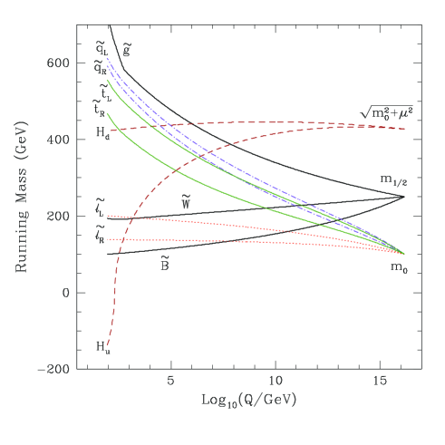
Indeed, it is rather amazing that from so few input parameters, all of the masses of the supersymmetric particles can be determined. The characteristic features that one sees in the figure, are for example, that the colored sparticles are typically the heaviest in the spectrum. This is due to the large positive correction to the masses due to $\alpha_{3}$ in the RGE’s. Also, one finds that the ${\widetilde{B}}$, is typically the lightest sparticle. But most importantly, notice that one of the Higgs mass², goes negative triggering electroweak symmetry breaking [31]. (The negative sign in the figure refers to the sign of the mass², even though it is the mass of the sparticles which are depicted.) In the Table below, I list some of the resultant electroweak scale masses, for the choice of parameters used in the figure.

Table 1: Physical mass parameters for $m_{1/2}=250$ GeV, $m_{0}=100$ GeV, $\tan\beta=3$, $A_{0}=0$, and $\mu<0$. (These are related but not equal to the running mass parameters shown in Figure 6.)

particle	mass	parameter	value
$m_{{\tilde{l}}}$	203	$\mu$	-391
$m_{{\tilde{e}}^{c}}$	144	$M_{1}$	100
$m_{{\tilde{\nu}}}$	190	$M_{2}$	193
$m_{{\tilde{q}}}$	412–554	$M_{3}$	726
$m_{{\tilde{\chi}}_{1}}$	104	$\alpha_{3}(M_{Z})$	.123
$m_{{\tilde{\chi}}^{\pm}_{1}}$	203	$A^{\prime}s$	163–878
$m_{h}$	93
$m_{A}$	466

4.3 Supergravity

Up until now, we have only considered global supersymmetry. Recall, our generator of supersymmetry transformations, the spinor $\xi$. In all of the derivations of the transformation and invariance properties in the first two sections, we had implicitly assumed that $\partial_{\mu}\xi=0$. By allowing $\xi(x)$ and $\partial_{\mu}\xi(x)\neq 0$, we obtain local supersymmetry or supergravity [36]. It is well beyond the means of these lectures to give a thorough treatment of local supersymmetry. We will therefore have to content ourself with some general remarks from which we can glimpse at some features for which we can expect will have some phenomenological relevance.

First, it is important to recognize that our original Lagrangian for the Wess-Zumino model involving a single noninteracting chiral multiplet will no longer be invariant under local supersymmetry transformations. New terms, proportional to $\partial_{\mu}\xi(x)$ must be canceled. In analogy with gauge, theories which contain similar terms and are canceled by the introduction of vector bosons, here the terms must be canceled by introducing a new spin 3/2 particle called the gravitino. The supersymmetry transformation property of the gravitino must be

$$\delta_{\xi}\Psi_{\mu}^{\alpha}\propto\partial_{\mu}\xi^{\alpha}$$ (148)

Notice that the gravitino carries both a gauge and a spinor index. The gravitino is part of an $N=1$ multiplet which contains the spin two graviton. In unbroken supergravity, the massless gravitino has two spin components ($\pm$ 3/2) to match the two polarization states of the graviton.

The scalar potential is now determined by a analytic function of the scalar fields, called the Kähler potential, $K(\phi,\phi^{*})$. The Kähler potential can be thought of as a metric in field space,

$${\cal L}_{kin}=K^{i}_{j}\partial_{\mu}\phi_{i}\partial^{\mu}{\phi^{j}}^{*}$$ (149)

where $K^{i}=\partial K/\partial\phi_{i}$ and $K_{i}=\partial K/\partial{\phi^{i}}^{*}$. In what is known as minimal $N=1$ supergravity, the Kähler potential is given by

$$K=\kappa^{2}\phi_{i}{\phi^{i}}^{*}+\ln(\kappa^{6}|W|^{2})$$ (150)

where $W(\phi)$ is the superpotential, $\kappa^{-1}=M_{P}/\sqrt{8\pi}$ and the Planck mass is $M_{P}=1.2\times 10^{19}$ GeV. The scalar potential (neglecting any gauge contributions) is [37]

$$V(\phi,\phi^{*})=e^{K}\kappa^{-4}\left[K^{i}(K^{-1})^{j}_{i}K_{j}-3\right]$$ (151)

For minimal supergravity, we have $K^{i}=\kappa^{2}{\phi^{i}}^{*}+{W^{i}}/W$, $K_{i}=\kappa^{2}\phi_{i}+W_{i}^{*}/W^{*}$, and $({K^{-1}})^{j}_{i}=\delta^{j}_{i}/\kappa^{2}$. Thus the resulting scalar potential is

$$V(\phi,\phi^{*})=e^{\kappa^{2}\phi_{i}{\phi^{i}}^{*}}\left[|W^{i}+{\phi^{i}}^{*}W|^{2}-3\kappa^{2}|W|^{2}\right]$$ (152)

As we will now see, one of the primary motivations for the CMSSM, and scalar mass universality comes from the simplest model for local supersymmetry breaking. The model [38] involves one additional chiral multiplet $z$, (above the normal matter fields $\phi_{i}$). Let us consider therefore, a superpotential which is separable in the so-called Polonyi field and matter so that

$$W(z,\phi_{i})=f(z)+g(\phi_{i})$$ (153)

and in particular let us choose

$$f(z)=\mu(z+\beta)$$ (154)

and for reasons to be clear shortly, $\beta=2-\sqrt{3}$. I will from now on work in units such that $\kappa=1$. If we ignore for the moment the matter fields $\phi$, the potential for $z$ becomes

$$V(z,z^{*})=e^{zz^{*}}\mu^{2}\left[|1+z^{*}(z+\beta)|^{2}-3|(z+\beta)|^{2}\right]$$ (155)

It is not difficult to verify that with the above choice of $\beta$, the minimum of $V$ occurs at $\langle z\rangle=\sqrt{3}-1$, with $V(\langle z\rangle)=0$.

Note that by expanding this potential, one can define two real scalar fields $A$ and $B$, with mass eigenvalues,

$$m_{A}^{2}=2\sqrt{3}m_{3/2}^{2}\qquad m_{B}^{2}=2(2-\sqrt{3})m_{3/2}^{2}$$ (156)

where the gravitino mass is

$$m_{3/2}=e^{K/2}=e^{2-\sqrt{3}}\mu$$ (157)

Note also that there is a mass relation, $m_{A}^{2}+m_{B}^{2}=4m_{3/2}^{2}$, which is a guaranteed consequence of supertrace formulae in supergravity [37]. Had we considered the fermionic sector of the theory, we would now find that the massive gravitino has four helicity states $\pm 1/2$ and $\pm 3/2$. The “longitudinal” states arise from the disappearance of the goldstino (the fermionic partner of $z$ in this case) by the superHiggs mechanism, again in analogy with the spontaneous breakdown of a gauge symmetry [39, 37, 38].

We next consider the matter potential from eqs. (153) and (152). In full, this takes the form [40]

$$V = e^{(|z|^{2}+|\phi|^{2})}\left[|{\partial f\over\partial z}+z^{*}(f(z)+g(\phi))|^{2}\right.$$ (158)

$$+\left.|{\partial g\over\partial\phi}+\phi^{*}(f(z)+g(\phi))|^{2}-3|f(z)+g(\phi)|^{2}\right]$$

Here again, I have left out the explicit powers of $M_{P}$. Expanding this expression, and at the same time dropping terms which are suppressed by inverse powers of the Planck scale (this can be done by simply dropping terms of mass dimension greater than four), we have, after inserting the vev for $z$ [40],

$$V = e^{(4-2\sqrt{3})}\left[|\mu+(\sqrt{3}-1)(\mu+g(\phi))|^{2}\right.$$ (159)

$$\left.+|{\partial g\over\partial\phi}+\phi^{*}(\mu+g(\phi))|^{2}-3|\mu+g(\phi)|^{2}\right]$$

$$= e^{(4-2\sqrt{3})}\left[-\sqrt{3}\mu(g(\phi)+g^{*}(\phi^{*}))+|{\partial g\over\partial\phi}|^{2}\right.$$

$$+\left.(\mu(\phi{\partial g\over\partial\phi}+\phi^{*}{\partial g^{*}\over\partial\phi^{*}})+\mu^{2}\phi\phi^{*}\right]$$

$$= e^{(4-2\sqrt{3})}|{\partial g\over\partial\phi}|^{2}$$

$$+m_{3/2}e^{(2-\sqrt{3})}(\phi{\partial g\over\partial\phi}-\sqrt{3}g+h.c.))+m_{3/2}^{2}\phi\phi^{*}$$

This last expression deserves some discussion. First, up to an overall rescaling of the superpotential, $g\to e^{\sqrt{3}-2}g$, the first term is the ordinary $F$-term part of the scalar potential of global supersymmetry. The next term, proportional to $m_{3/2}$ represents a universal trilinear $A$-term. This can be seen by noting that $\sum\phi\partial g/\partial\phi=3g$, so that in this model of supersymmetry breaking, $A=(3-\sqrt{3})m_{3/2}$. Note that if the superpotential contains bilinear terms, we would find $B=(2-\sqrt{3})m_{3/2}$. The last term represents a universal scalar mass of the type advocated in the CMSSM, with $m_{0}^{2}=m_{3/2}^{2}$. The generation of such soft terms is a rather generic property of low energy supergravity models [41].

Before concluding this section, it worth noting one other class of supergravity models, namely the so-called no-scale supergravity model [42]. No-scale supergravity is based on the Kähler potential of the form

$$K=-\ln(S+S^{*})-3\ln(T+T^{*}-\phi_{i}{\phi^{i}}^{*})+\ln|W|^{2}$$ (160)

where the $S$ and $T$ fields are related to the dilaton and moduli fields in string theory [43]. If only the $T$ field is kept in (160), the resulting scalar potential is exactly flat, i.e., $V=0$ identically. In such a model, the gravitino mass is undetermined at the tree level, and up to some field redefinitions, there is a surviving global supersymmetry. No-scale supergravity has been used heavily in constructing supergravity models in which all mass scales below the Planck scale are determined radiatively [44],[45].

5 Cosmology

Supersymmetry has had a broad impact on cosmology. In these last two lectures, I will try to highlight these. In this lecture, I will briefly review the problems induced by supersymmetry, such as the Polonyi or moduli problem, and the gravitino problem. I will also discuss the question of cosmological inflation in the context of supersymmetry. Finally, I will describe a mechanism for baryogenesis which is purely supersymmetric in origin. I will leave the question of dark matter and the accelerator constraints to the last lecture.

Before proceeding to the problems, it will be useful to establish some of the basic quantities and equations in cosmology. The standard big bang model assumes homogeneity and isotropy, so that space-time can be described by the Friedmann-Robertson-Walker metric which in co-moving coordinates is given by

$$ds^{2}=-dt^{2}+R^{2}(t)\left[{dr^{2}\over\left(1-kr^{2}\right)}+r^{2}\left(d\theta^{2}+\sin^{2}\theta d\phi^{2}\right)\right]$$ (161)

where $R(t)$ is the cosmological scale factor and $k$ is the three-space curvature constant ($k=0,+1,-1$ for a spatially flat, closed or open Universe). $k$ and $R$ are the only two quantities in the metric which distinguish it from flat Minkowski space. It is also common to assume the perfect fluid form for the energy-momentum tensor

$$T_{\mu\nu}=pg_{\mu\nu}+(p+\rho)u_{\mu}u_{\nu}$$ (162)

where $g_{\mu\nu}$ is the space-time metric described by (161), $p$ is the isotropic pressure, $\rho$ is the energy density and $u^{\mu}=(1,0,0,0)$ is the velocity vector for the isotropic fluid. Einstein’s equation yield the Friedmann equation,

$$H^{2}\equiv\left({\dot{R}\over R}\right)^{2}={1\over 3}\kappa^{2}\rho-{k\over R^{2}}+{1\over 3}\Lambda$$ (163)

and

$$\left({\ddot{R}\over R}\right)={1\over 3}\Lambda-{1\over 6}\kappa^{2}(\rho+3p)$$ (164)

where $\Lambda$ is the cosmological constant, or equivalently from ${T^{\mu\nu}}_{;\nu}=0$

$$\dot{\rho}=-3H(\rho+p)$$ (165)

These equations form the basis of the standard big bang model.

If our Lagrangian contains scalar fields, then from the scalar field contribution to the energy-momentum tensor

$$T_{\mu\nu}=\partial_{\mu}\phi\partial_{\nu}\phi-{1\over 2}g_{\mu\nu}\partial_{\rho}\phi\partial^{\rho}\phi-g_{\mu\nu}V(\phi)$$ (166)

we can identify the energy density and pressure due to a scalar $\phi$,

$$\rho={1\over 2}{\dot{\phi}}^{2}+{1\over 2}R^{-2}(t)(\nabla\phi)^{2}+V(\phi)$$ (167)

$$p={1\over 2}{\dot{\phi}}^{2}-{1\over 6}R^{-2}(t)(\nabla\phi)^{2}-V(\phi)$$ (168)

In addition, we have the equation of motion,

$${\ddot{\phi}}+3H{\dot{\phi}}+{\partial V\over\partial\phi}=0$$ (169)

Finally, I remind the reader that in the early radiation dominated Universe, the energy density (as well as the Hubble parameter) is determined by the temperature,

$$\rho=N{\pi^{2}\over 30}T^{4}\qquad H=\sqrt{\pi^{2}N\over 90}\kappa{T^{2}}$$ (170)

The critical energy density (corresponding to $k=1$, is

$$\rho_{c}={3H^{2}\kappa^{-2}}=1.88\times 10^{-29}{\rm gcm}^{-3}h_{0}^{2}$$ (171)

where the scaled Hubble parameter is $h_{0}=H_{0}/100$km Mpc^-1s^-1. The cosmological density parameter is defined as $\Omega=\rho/\rho_{c}$.

5.1 The Polonyi Problem

The Polonyi problem, although based on the specific choice for breaking supergravity discussed in the previous lecture (eq. 154), is a generic problem in broken supergravity models. In fact, the problem is compounded in string theories, where there are in general many such fields called moduli. Here, attention will be restricted to the simple example of the Polonyi potential.

The potential in eq. (155) has the property that at its minimum occurs at $\langle z\rangle=(\sqrt{3}-1)M$, where $M=\kappa^{-1}$ is the reduced Planck mass. Recall that the constant $\beta$ was chosen so that at the minimum, $V(\langle z\rangle)=0$. In contrast to the value of the expectation value, the curvature of the potential at the minimum, is $m_{z}^{2}\sim\mu^{2}$, which as argued earlier is related to the gravitino mass and therefore must be of order the weak scale. In addition the value of the potential at the origin is of order $V(0)\sim\mu^{2}M^{2}$, i.e., an intermediate scale. Thus, we have a long and very flat potential.

Without too much difficulty, it is straightforward to show that such a potential can be very problematic cosmologically [46]. The evolution of the Polonyi field $z$, is governed by eq. (169) with potential (155). There is no reason to expect that the field $z$ is initially at its minimum. This is particularly true if there was a prior inflationary epoch, since quantum fluctuations for such a light field would be large, displacing the field by an amount of order $M$ from its minimum. If $z\neq\langle z\rangle$, the evolution of $z$ must be traced. When the Hubble parameter $H>\mu$ , $z$ is approximately constant. That is, the potential term (proportional to $\mu^{2}$) can be neglected. At later times, as $H$ drops, $z$ begins to oscillate about the minimum when $H\mathrel{\raise 1.29167pt\hbox{$<$\kern-7.5pt\lower 4.30554pt\hbox{$\sim$}}}\mu$. Generally, oscillations begin when $H\sim m_{z}\sim\mu$ as can be seen from the solution for the evolution of a non-interacting massive field with $V=m_{z}^{2}z^{2}/2$. This solution would take the form of $z\sim\sin(m_{z}t)/t$ with $H=2/3t$.

At the time that the $z$-oscillations begin, the Universe becomes dominated by the potential $V(z)$, since $H^{2}\sim\rho/M^{2}$. Therefore all other contributions to $\rho$ will redshift away, leaving the potential as the dominant component to the energy density. Since the oscillations evolve as non-relativistic matter (recall that in the above solution for $z$, $H=2/3t$ as in a matter dominated Universe). As the Universe evolves, we can express the energy density as $\rho\sim\mu^{2}M^{2}(R_{z}/R)^{3}$, where $R_{z}$ is the value of the scale factor when the oscillations begin. Oscillations continue, until the $z$-fields can decay. Since they are only gravitationally coupled to matter, their decay rate is given by $\Gamma_{z}\sim\mu^{3}/M^{2}$. Therefore oscillations continue until $H\sim\Gamma_{z}$ or when $R=R_{dz}\sim(M/\mu)^{4/3}$. The energy density at this time is only $\mu^{6}/M^{2}$. Even if the the thermalization of the decay products occurs rapidly, the Universe reheats only to a temperature of order $T_{R}\sim\rho^{1/4}\sim\mu^{3/2}/M^{1/2}$. For $\mu\sim 100$ GeV, we have $T_{R}\sim 100$ keV! There are two grave problems with this scenario. The first is is that big bang nucleosynthesis would have taken place during the oscillations which is characteristic of a matter dominated expansion rather than a radiation dominated one. Because of the difference in the expansion rate the abundances of the light elements would be greatly altered (see e.g. [47]). Even more problematic is the entropy release due to the decay of these oscillations. The entropy increase [46] is related to the ratio of the reheat temperature to the temperature of the radiation in the Universe when the oscillations decay, $T_{d}\sim T_{i}(R_{z}/R_{dz})$ where $T_{i}$ is the temperature when oscillations began $T_{i}\sim(\mu M)^{1/2}$. Therefore, the entropy increase is given by

$$S_{f}/S_{i}\sim(T_{R}/T_{d})^{3}\sim(M/\mu)\sim 10^{16}$$ (172)

This is far too much to understand the present value of the baryon-to-entropy ratio, of order $10^{-11}-10^{-10}$ as required by nucleosynthesis and allowed by baryosynthesis. That is, even if a baryon asymmetry of order one could be produced, a dilution by a factor of $10^{16}$ could not be accommodated.

5.2 The Gravitino Problem

Another problem which results from the breaking of supergravity is the gravitino problem [48]. If gravitinos are present with equilibrium number densities, we can write their energy density as

$$\rho_{3/2}=m_{3/2}n_{3/2}=m_{3/2}\left(3\zeta(3)\over\pi^{2}\right)T_{3/2}^{2}$$ (173)

where today one expects that the gravitino temperature $T_{3/2}$ is reduced relative to the photon temperature due to the annihilations of particles dating back to the Planck time [49]. Typically one can expect $Y_{3/2}=(T_{3/2}/T_{\gamma})^{3}\sim 10^{-2}$. Then for $\Omega_{3/2}h^{2}\mathrel{\raise 1.29167pt\hbox{$<$\kern-7.5pt\lower 4.30554pt\hbox{$\sim$}}}1$, we obtain the limit that $m_{3/2}\mathrel{\raise 1.29167pt\hbox{$<$\kern-7.5pt\lower 4.30554pt\hbox{$\sim$}}}1$ keV.

Of course, the above mass limits assumes a stable gravitino, the problem persists however, even if the gravitino decays, since its gravitational decay rate is very slow. Gravitinos decay when their decay rate, $\Gamma_{3/2}\simeq m_{3/2}^{3}/M_{P}^{2}$, becomes comparable to the expansion rate of the Universe (which becomes dominated by the mass density of gravitinos), $H\simeq m_{3/2}^{1/2}T_{3/2}^{3/2}/M_{P}$. Thus decays occur at $T_{d}\simeq m_{3/2}^{5/3}/M_{P}^{2/3}$. After the decay, the Universe is “reheated” to a temperature

$$T_{R}\simeq\rho(T_{d})^{1/4}\simeq m_{3/2}^{3/2}/M_{P}^{1/2}$$ (174)

As in the case of the decay of the Polonyi fields, the Universe must reheat sufficiently so that big bang nucleosynthesis occurs in a standard radiation dominated Universe. For $T_{R}\mathrel{\raise 1.29167pt\hbox{$>$\kern-7.5pt\lower 4.30554pt\hbox{$\sim$}}}1$ MeV, we must require $m_{3/2}\mathrel{\raise 1.29167pt\hbox{$>$\kern-7.5pt\lower 4.30554pt\hbox{$\sim$}}}20$ TeV. This large value threatens the solution of the hierarchy problem. In addition, one must still be concerned about the dilution of the baryon-to-entropy ratio [50], in this case by a factor $\Delta=(T_{R}/T_{D})^{3}\sim Y(M_{P}/m_{3/2})^{1/2}$. Dilution may not be a problem if the baryon-to-entropy ratio is initially large.

Inflation (discussed below) could alleviate the gravitino problem by diluting the gravitino abundance to safe levels [50]. If gravitinos satisfy the noninflationary bounds, then their reproduction after inflation is never a problem. For gravitinos with mass of order 100 GeV, dilution without over-regeneration will also solve the problem, but there are several factors one must contend with in order to be cosmologically safe. Gravitino decay products can also upset the successful predictions of Big Bang nucleosynthesis, and decays into LSPs (if R-parity is conserved) can also yield too large a mass density in the now-decoupled LSPs [19]. For unstable gravitinos, the most restrictive bound on their number density comes form the photo-destruction of the light elements produced during nucleosynthesis [51]

$$n_{3/2}/n_{\gamma}\mathrel{\raise 1.29167pt\hbox{$<$\kern-7.5pt\lower 4.30554pt\hbox{$\sim$}}}10^{-13}(100{\rm GeV}/m_{3/2})$$ (175)

for lifetimes $>10^{4}$ sec. Gravitinos are regenerated after inflation and one can estimate [19, 50, 51]

$$n_{3/2}/n_{\gamma}\sim(\Gamma/H)(T_{3/2}/T_{\gamma})^{3}\sim\alpha N(T_{R})(T_{R}/M_{P})(T_{3/2}/T_{\gamma})^{3}$$ (176)

where $\Gamma\sim\alpha N(T_{R})(T_{R}^{3}/M_{P}^{2})$ is the production rate of gravitinos. Combining these last two equations one can derive bounds on $T_{R}$

$$T_{R}\mathrel{\raise 1.29167pt\hbox{$<$\kern-7.5pt\lower 4.30554pt\hbox{$\sim$}}}4\times 10^{9}~{}{\rm GeV}(100~{}{\rm GeV}/m_{3/2})$$ (177)

using a more recent calculation of the gravitino regeneration rate [52]. A slightly stronger bound (by an order of magnitude in $T_{R}$) was found in [53].

5.3 Inflation

It would be impossible in the context of these lectures to give any kind of comprehensive review of inflation whether supersymmetric or not. I refer the reader to several reviews [54]. Here I will mention only the most salient features of inflation as it connects with supersymmetry.

Supersymmetry was first introduced [55] in inflationary models as a means to cure some of the problems associated with the fine-tuning of new inflation [56]. New inflationary models based on a Coleman-Weinberg type of $SU(5)$ breaking produced density fluctuations [57] with magnitude $\delta\rho/\rho\sim O(10^{2})$ rather than $\delta\rho/\rho\sim 10^{-5}$ as needed to remain consistent with microwave background anisotropies. Other more technical problems[58] concerning slow rollover and the effects of quantum fluctuations also passed doom on this original model.

The problems associated with new inflation, had to with the interactions of the scalar field driving inflation, namely the $SU(5)$ adjoint. One cure is to (nearly) completely decouple the field driving inflation, the inflaton, from the gauge sector. As gravity becomes the primary interaction to be associated with the inflaton it seemed only natural to take all scales to be the Planck scale [55]. Supersymmetry was also employed to give flatter potentials and acceptable density perturbations[59]. These models were then placed in the context of N=1 supergravity[60, 61].

The simplest such model for the inflaton $\eta$, is based on a superpotential of the form

$$W(\eta)=\mu^{2}(1-\eta/M_{P})^{2}M_{P}$$ (178)

or

$$W(\eta)=\mu^{2}(\eta-\eta^{4}/4{M_{P}}^{3})$$ (179)

where Eq.(178)[61] is to be used in minimal supergravity while Eq.(179)[62] is to be used in no-scale supergravity. Of course the real goal is to determine the identity of the inflaton. Presumably string theory holds the answer to this question, but a fully string theoretic inflationary model has yet to be realized [63].

For the remainder of the discussion, it will be sufficient to consider only a generic model of inflation whose potential is of the form:

$$V(\eta)={{\mu}^{4}}P(\eta)$$ (180)

where $\eta$ is the scalar field driving inflation, the inflaton, $\mu$ is an as yet unspecified mass parameter, and $P(\eta)$ is a function of $\eta$ which possesses the features necessary for inflation, but contains no small parameters, i.e., where all of the couplings in $P$ are $O(1)$ but may contain non-renormalizable terms.

The requirements for successful inflation can be expressed in terms of two conditions: 1) enough inflation;

$${\partial^{2}V\over\partial\eta^{2}}\mid_{\eta\sim{\eta_{i}}\pm H}<{3H^{2}\over 65}={8\pi V(0)\over 65{M_{P}}^{2}}$$ (181)

2) density perturbations of the right magnitude[57];

$${\delta\rho\over\rho}\simeq{H^{2}\over 10\pi^{3/2}\dot{\eta}}\simeq O(100){\mu^{2}\over{M_{P}}^{2}}$$ (182)

given here for scales which “re-enter” the horizon during the matter dominated era. For large scale fluctuations of the type measured by COBE[64], we can use Eq. (182) to fix the inflationary scale $\mu$ [65]:

$${\frac{\mu^{2}}{M_{P}^{2}}={\rm few}\times{10^{-8}}}$$ (183)

Fixing $({\mu^{2}}/{M_{P}^{2}})$ has immediate general consequences for inflation[66]. For example, the Hubble parameter during inflation, ${{H^{2}}\simeq(8\pi/3)({\mu^{4}}/{M_{P}^{2}})}$ so that $H\sim 10^{-7}M_{P}$. The duration of inflation is $\tau\simeq{M_{P}^{3}}/{\mu^{4}}$, and the number of e-foldings of expansion is $H\tau\sim 8\pi({M_{P}^{2}}/{\mu^{2}})\sim 10^{9}$. If the inflaton decay rate goes as $\Gamma\sim{m_{\eta}^{3}}/{M_{P}^{2}}\sim{\mu^{6}}/{M_{P}^{5}}$, the universe recovers at a temperature $T_{R}\sim(\Gamma{M_{P}})^{1/2}\sim{\mu^{3}}/{M_{P}^{2}}\sim 10^{-11}{M_{P}}\sim 10^{8}GeV$. However, it was noted in [66] that in fact the Universe is not immediately thermalized subsequent to inflaton decays, and the process of thermalization actually leads to a smaller reheating temperature,

$$T_{R}\sim\alpha^{2}\mu^{3}/M_{P}^{2}\sim 10^{5}GeV~{},$$ (184)

where $\alpha^{2}\sim 10^{-3}$ characterizes the strength of the interactions leading to thermalization. This low reheating temperature is certainly safe with regards to the gravitino limit (177) discussed above.

5.4 Baryogenesis

The production of a net baryon asymmetry requires baryon number violating interactions, C and CP violation and a departure from thermal equilibrium[67]. The first two of these ingredients are contained in GUTs, the third can be realized in an expanding universe where it is not uncommon that interactions come in and out of equilibrium.

In the original and simplest model of baryogenesis [68], a GUT gauge or Higgs boson decays out of equilibrium producing a net baryon asymmetry. While the masses of the gauge bosons is fixed to the rather high GUT scale $10^{15-16}$ GeV, the masses of the triplets could be lighter $O(10^{10})$ GeV and still remain compatible with proton decay because of the Yukawa suppression in the proton decay rate when mediated by a heavy Higgs. This reduced mass allows the simple out-out-equilibrium decay scenario to proceed after inflation so long as the Higgs is among the inflaton decay products [69]. From the arguments above, an inflaton mass of $10^{11}$ GeV is sufficient to realize this mechanism. Higgs decays in this mechanism would be well out of equilibrium as at reheating $T\ll m_{H}$ and $n_{H}\sim n_{\gamma}$. In this case, the baryon asymmetry is given simply by

$${n_{B}\over s}\sim\epsilon{n_{H}\over{T_{R}}^{3}}\sim\epsilon{n_{\eta}\over{T_{R}}^{3}}\sim\epsilon{T_{R}\over m_{\eta}}\sim\epsilon\left({m_{\eta}\over M_{P}}\right)^{1/2}\sim\epsilon{\mu\over M_{P}}\sim 10^{-4}\epsilon$$ (185)

where $\epsilon$ is the CP violation in the decay, $T_{R}$ is the reheat temperature after inflation, and I have substituted for $n_{\eta}=\rho_{\eta}/m_{\eta}\sim\Gamma^{2}{M_{P}}^{2}/m_{\eta}$.

In a supersymmetric grand unified SU(5) theory, the superpotential $F_{Y}$ must be expressed in terms of SU(5) multiplets

$$F_{Y}=h_{d}{\bf H_{2}~{}{\bar{5}}~{}10}+h_{u}{\bf H_{1}~{}10~{}10}$$ (186)

where $10,{\bar{5}},H_{1}$ and $H_{2}$ are chiral supermultiplets for the 10 and ${\bar{5}}$-plets of SU(5) matter fields and the Higgs 5 and ${\bar{5}}$ multiplets respectively. There are now new dimension 5 operators [25, 70] which violate baryon number and lead to proton decay as shown in Figure 7. The first of these diagrams leads to effective dimension 5 Lagrangian terms such as

$${\cal L}_{\rm eff}^{(5)}={h_{u}h_{d}\over M_{H}}(\tilde{q}\tilde{q}ql)$$ (187)

and the resulting dimension 6 operator for proton decay [71]

$${\cal L}_{\rm eff}={h_{u}h_{d}\over M_{H}}\left({g^{2}\over M_{\tilde{G}}}\right)(qqql)$$ (188)

As a result of diagrams such as these, the proton decay rate scales as $\Gamma\sim h^{4}g^{4}/M_{H}^{2}M_{\tilde{G}}^{2}$ where $M_{H}$ is the triplet mass, and $M_{\tilde{G}}$ is a typical gaugino mass of order $\mathrel{\raise 1.29167pt\hbox{$<$\kern-7.5pt\lower 4.30554pt\hbox{$\sim$}}}$ 1 TeV. This rate however is much too large unless $M_{H}\mathrel{\raise 1.29167pt\hbox{$>$\kern-7.5pt\lower 4.30554pt\hbox{$\sim$}}}10^{16}$ GeV.

Figure 7: Dimension 5 and induced dimension 6 graphs violating baryon number.

It is however possible to have a lighter ($O(10^{10}-10^{11})$ GeV) Higgs triplet needed for baryogenesis in the out-of-equilibrium decay scenario with inflation. One needs two pairs of Higgs five-plets ($H_{1},H_{2}$ and $H_{1}^{\prime},H_{2}^{\prime}$ which is anyway necessary to have sufficient C and CP violation in the decays. By coupling one pair $(H_{2}$ and $H_{1}^{\prime})$ only to the third generation of fermions via [72]

$$a{\bf H_{1}1010}+b{\bf H_{1}^{\prime}10_{3}10_{3}}+c{\bf H_{2}10_{3}{\bar{5}}_{3}}+d{\bf H_{2}^{\prime}10{\bar{5}}}$$ (189)

proton decay can not be induced by the dimension five operators.

5.4.1 The Affleck-Dine Mechanism

Another mechanism for generating the cosmological baryon asymmetry is the decay of scalar condensates as first proposed by Affleck and Dine[73]. This mechanism is truly a product of supersymmetry. It is straightforward though tedious to show that there are many directions in field space such that the scalar potential given in eq. (78) vanishes identically when SUSY is unbroken. That is, with a particular assignment of scalar vacuum expectation values, $V=0$ in both the $F-$ and $D-$ terms. An example of such a direction is

$$u_{3}^{c}=a\qquad s_{2}^{c}=a\qquad-u_{1}=v\qquad\mu^{-}=v\qquad b_{1}^{c}=e^{i\phi}\sqrt{v^{2}+a^{2}}$$ (190)

where $a,v$ are arbitrary complex vacuum expectation values. SUSY breaking lifts this degeneracy so that

$$V\simeq\tilde{m}^{2}\phi^{2}$$ (191)

where $\tilde{m}$ is the SUSY breaking scale and $\phi$ is the direction in field space corresponding to the flat direction. For large initial values of $\phi$,  $\phi_{o}\sim M_{gut}$, a large baryon asymmetry can be generated[73, 74]. This requires the presence of baryon number violating operators such as $O=qqql$ such that $\langle O\rangle\neq 0$. The decay of these condensates through such an operator can lead to a net baryon asymmetry.

In a supersymmetric gut, as we have seen above, there are precisely these types of operators. In Figure 8, a 4-scalar diagram involving the fields of the flat direction (190) is shown. Again, $\tilde{G}$ is a (light) gaugino, and ${\widetilde{X}}$ is a superheavy gaugino. The two supersymmetry breaking insertions are of order $\tilde{m}$, so that the diagram produces an effective quartic coupling of order ${\tilde{m}}^{2}/(\phi_{o}^{2}+M_{X}^{2})$.

Figure 8: Baryon number violating diagram involving flat direction fields.

The baryon asymmetry is computed by tracking the evolution of the sfermion condensate, which is determined by

$$\ddot{\phi}+3H\dot{\phi}=-{\tilde{m}}^{2}\phi$$ (192)

To see how this works, it is instructive to consider a toy model with potential [74]

$$V(\phi,\phi^{*})=\tilde{m}^{2}\phi\phi^{*}+{1\over 2}i\lambda[\phi^{4}-{\phi^{*}}^{4}]$$ (193)

The equation of motion becomes

$$\ddot{\phi_{1}}+3H\dot{\phi_{1}}=-{\tilde{m}}^{2}\phi_{1}+3\lambda\phi_{1}^{2}\phi_{2}-\lambda\phi_{2}^{3}$$ (194)

$$\ddot{\phi_{2}}+3H\dot{\phi_{2}}=-{\tilde{m}}^{2}\phi_{2}-3\lambda\phi_{2}^{2}\phi_{1}+\lambda\phi_{1}^{3}$$ (195)

with $\phi=(\phi_{1}+i\phi_{2})/\sqrt{2}$. Initially, when the expansion rate of the Universe, $H$, is large, we can neglect $\ddot{\phi}$ and $\tilde{m}$. As one can see from (193) the flat direction lies along $\phi\simeq\phi_{1}\simeq\phi_{o}$ with $\phi_{2}\simeq 0$. In this case, $\dot{\phi_{1}}\simeq 0$ and $\dot{\phi_{2}}\simeq{\lambda\over 3H}\phi_{o}^{3}$. Since the baryon density can be written as $n_{B}=j_{o}={1\over 2}(\phi_{1}\dot{\phi_{2}}-\phi_{2}\dot{\phi_{1}})\simeq{\lambda\over 6H}\phi_{o}^{4}$, by generating some motion in the imaginary $\phi$ direction, we have generated a net baryon density.

When $H$ has fallen to order $\tilde{m}$ (when $t^{-1}\sim\tilde{m}$), $\phi_{1}$ begins to oscillate about the origin with $\phi_{1}\simeq\phi_{o}\sin(\tilde{m}t)/\tilde{m}t$. At this point the baryon number generated is conserved and the baryon density, $n_{B}$ falls as $R^{-3}$. Thus,

$$n_{B}\sim{\lambda\over\tilde{m}}\phi_{o}^{2}\phi^{2}\propto R^{-3}$$ (196)

and relative to the number density of $\phi$’s ($n_{\phi}=\rho_{\phi}/\tilde{m}=\tilde{m}\phi^{2}$)

$${n_{B}\over n_{\phi}}\simeq{\lambda\phi_{o}^{2}\over{\tilde{m}}^{2}}$$ (197)

If it is assumed that the energy density of the Universe is dominated by $\phi$, then the oscillations will cease, when

$$\Gamma_{\phi}\simeq{{\tilde{m}}^{3}\over\phi^{2}}\simeq H\simeq{\rho_{\phi}^{1/2}\over M_{P}}\simeq{{\tilde{m}}\phi\over M_{P}}$$ (198)

or when the amplitude of oscillations has dropped to $\phi_{D}\simeq(M_{P}{\tilde{m}}^{2})^{1/3}$. Note that the decay rate is suppressed as fields coupled directly to $\phi$ gain masses $\propto\phi$. It is now straightforward to compute the baryon to entropy ratio,

$${n_{B}\over s}={n_{B}\over\rho_{\phi}^{3/4}}\simeq{\lambda\phi_{o}^{2}\phi_{D}^{2}\over{\tilde{m}}^{5/2}\phi_{D}^{3/2}}={\lambda\phi_{o}^{2}\over{\tilde{m}}^{2}}\left({M_{P}\over\tilde{m}}\right)^{1/6}$$ (199)

and after inserting the quartic coupling

$${n_{B}\over s}\simeq\epsilon{\phi_{o}^{2}\over(M_{X}^{2}+\phi_{o}^{2})}\left({M_{P}\over\tilde{m}}\right)^{1/6}$$ (200)

which could be $O(1)$.

In the context of inflation, a couple of significant changes to the scenario take place. First, it is more likely that the energy density is dominated by the inflaton rather than the sfermion condensate. The sequence of events leading to a baryon asymmetry is then as follows [66]: After inflation, oscillations of the inflaton begin at $R=R_{\eta}$ when $H\sim m_{\eta}$ and oscillations of the sfermions begin at $R=R_{\phi}$ when $H\sim{\tilde{m}}$. If the Universe is inflaton dominated, $H\sim m_{\eta}(R_{\eta}/R)^{3/2}$ since $H\sim\rho_{\eta}^{1/2}$ and $\rho_{\eta}\sim\eta^{2}\sim R^{-3}$ Thus one can relate $R_{\eta}$ and $R_{\phi}$, $R_{\phi}\simeq(m_{\eta}/{\tilde{m}})^{2/3}R_{\eta}$. As discussed earlier, inflatons decay when $\Gamma_{\eta}=m_{\eta}^{3}/M_{P}^{2}=H$ or when $R=R_{d\eta}\simeq(M_{p}/m_{\eta})^{4/3}R_{\eta}$. The Universe then becomes dominated by the relativistic decay products of the inflaton, $\rho_{r\eta}=m_{\eta}^{2/3}M_{P}^{10/3}(R_{\eta}/R)^{4}$ and $H=m_{\eta}^{1/3}M_{P}^{2/3}(R_{\eta}/R)^{2}$. Sfermion decays still occur when $\Gamma_{\phi}=H$ which now corresponds to a value of the scale factor $R_{d\phi}=(m_{\eta}^{7/15}\phi_{o}^{2/5}M_{P}^{2/15}/{\tilde{m}})R_{\eta}$. The final baryon asymmetry in the Affleck-Dine scenario with inflation becomes [66]

$$\frac{n_{B}}{s}\sim\frac{\epsilon{\phi_{o}}^{4}{m_{\eta}}^{3/2}}{{M_{X}}^{2}{M_{P}}^{5/2}\tilde{m}}\sim\frac{\epsilon m_{\eta}^{7/2}}{{M_{X}}^{2}{M_{P}}^{1/2}\tilde{m}}\sim(10^{-6}-1)\epsilon$$ (201)

for $\tilde{m}\sim(10^{-17}-10^{-16})M_{P}$, and $M_{X}\sim(10^{-4}-10^{-3})M_{P}$ and $m_{\eta}\sim(10^{-8}-10^{-7})M_{P}$.

When combined with inflation, it is important to verify that the AD flat directions remain flat. In general, during inflation, supersymmetry is broken. The gravitino mass is related to the vacuum energy and $m_{3/2}^{2}\sim V/M_{P}^{2}\sim H^{2}$, thus lifting the flat directions and potentially preventing the realization of the AD scenario as argued in [75]. To see this, recall the minimal supergravity model defined in eqs. (150) - (153). Recall also, the last term in eq. (159), which gives a mass to all scalars (in the matter sector), including flat directions of order the gravitino mass which during inflation is large. This argument can be generalized to supergravity models with non-minimal Kähler potentials.

However, in no-scale supergravity models, or more generally in models which possess a Heisenberg symmetry [76], the Kähler potential can be written as (cf. eq. (160))

$$G=f(z+z^{*}-\phi_{i}^{*}\phi^{i})+\ln|W(\phi)|^{2}$$ (202)

Now, one can write

$$V=e^{f(\eta)}\left[\left(\frac{f^{\prime 2}}{f^{\prime\prime}}-3\right)|W|^{2}-\frac{1}{f^{\prime}}|W_{i}|^{2}\right]$$ (203)

It is important to notice that the cross term $|\phi_{i}^{*}W|^{2}$ has disappeared in the scalar potential. Because of the absence of the cross term, flat directions remain flat even during inflation [77]. The no-scale model corresponds to $f=-3\ln\eta$, $f^{\prime 2}=3f^{\prime\prime}$ and the first term in (203) vanishes. The potential then takes the form

$$V=\left[\frac{1}{3}e^{{2\over 3}f}|W_{i}|^{2}\right],$$ (204)

which is positive definite. The requirement that the vacuum energy vanishes implies $\langle W_{i}\rangle=\langle g_{a}\rangle=0$ at the minimum. As a consequence $\eta$ is undetermined and so is the gravitino mass $m_{3/2}(\eta)$.

The above argument is only valid at the tree level. An explicit one-loop calculation [78] shows that the effective potential along the flat direction has the form

$$V_{eff}\sim\frac{g^{2}}{(4\pi)^{2}}\langle V\rangle\left(-2\phi^{2}\log\left(\frac{\Lambda^{2}}{g^{2}\phi^{2}}\right)+\phi^{2}\right)+{\cal O}(\langle V\rangle)^{2},$$ (205)

where $\Lambda$ is the cutoff of the effective supergravity theory, and has a minimum around $\phi\simeq 0.5\Lambda$. Thus, $\phi_{0}\sim M_{P}$ will be generated and in this case the subsequent sfermion oscillations will dominate the energy density and a baryon asymmetry will result which is independent of inflationary parameters as originally discussed in [73, 74] and will produce $n_{B}/s\sim O(1)$. Thus we are left with the problem that the baryon asymmetry in no-scale type models is too large [79, 77, 80].

In [80], several possible solutions were presented to dilute the baryon asymmetry. These included 1) entropy production from moduli decay, 2) the presence of non-renormalizable interactions, and 3) electroweak effects. Moduli decay in this context, turns out to be insufficient to bring an initial asymmetry of order $n_{B}/s\sim 1$ down to acceptable levels. However, as a by-product one can show that there is no moduli problem either. In contrast, adding non-renormalizable Planck scale operators of the form $\phi^{2n-2}/M_{P}^{2n-6}$ leads to a smaller initial value for $\phi_{o}$ and hence a smaller value for $n_{B}/s$. For dimension 6 operators ($n=4$), a baryon asymmetry of order $n_{B}/s\sim 10^{-10}$ is produced. Finally, another possible suppression mechanism is to employ the smallness of the fermion masses. The baryon asymmetry is known to be wiped out if the net $B-L$ asymmetry vanishes because of the sphaleron transitions at high temperature. However, Kuzmin, Rubakov and Shaposhnikov [81] pointed out that this erasure can be partially circumvented if the individual $(B-3L_{i})$ asymmetries, where $i=1,2,3$ refers to three generations, do not vanish even when the total asymmetry vanishes. Even though there is still a tendency that the baryon asymmetry is erased by the chemical equilibrium due to the sphaleron transitions, the finite mass of the tau lepton shifts the chemical equilibrium between $B$ and $L_{3}$ towards the $B$ side and leaves a finite asymmetry in the end. Their estimate is

$$B=-\frac{4}{13}\sum_{i}\left(L_{i}-\frac{1}{3}B\right)\left(1+\frac{1}{\pi^{2}}\frac{m_{l_{i}}^{2}}{T^{2}}\right)$$ (206)

where the temperature $T\sim T_{C}\sim 200$ GeV is when the sphaleron transition freezes out (similar to the temperature of the electroweak phase transition) and $m_{\tau}(T)$ is expected to be somewhat smaller than $m_{\tau}(0)=1.777$ GeV. Overall, the sphaleron transition suppresses the baryon asymmetry by a factor of $\sim 10^{-6}$. This suppression factor is sufficient to keep the total baryon asymmetry at a reasonable order of magnitude in many of the cases discussed above.

6 Dark Matter and Accelerator Constraints

There is considerable evidence for dark matter in the Universe [82]. The best observational evidence is found on the scale of galactic halos and comes from the observed flat rotation curves of galaxies. There is also good evidence for dark matter in elliptical galaxies, as well as clusters of galaxies coming from X-ray observations of these objects. In theory, we expect dark matter because 1) inflation predicts $\Omega=1$, and the upper limit on the baryon (visible) density of the Universe from big bang nucleosynthesis is $\Omega_{B}<0.1$ [83]; 2) Even in the absence of inflation (which does not distinguish between matter and a cosmological constant), the large scale power spectrum is consistent with a cosmological matter density of $\Omega\sim 0.3$, still far above the limit from nucleosynthesis; and 3) our current understanding of galaxy formation is inconsistent with observations if the Universe is dominated by baryons.

It is also evident that not only must there be dark matter, the bulk of the dark matter must be non-baryonic. In addition to the problems with baryonic dark matter associated with nucleosynthesis or the growth of density perturbations, it is very difficult to hide baryons. There are indeed very good constraints on the possible forms for baryonic dark matter in our galaxy. Strong cases can be made against hot gas, dust, jupiter size objects, and stellar remnants such as white dwarfs and neutron stars [84].

In what follows, I will focus on the region of the parameter space in which the relic abundance of dark matter contributes a significant though not excessive amount to the overall energy density. Denoting by $\Omega_{\chi}$ the fraction of the critical energy density provided by the dark matter, the density of interest falls in the range

$$0.1\leq\Omega_{\chi}h^{2}\leq 0.3$$ (207)

The lower limit in eq.(207) is motivated by astrophysical relevance. For lower values of $\Omega_{\chi}h^{2}$, there is not enough dark matter to play a significant role in structure formation, or constitute a large fraction of the critical density. The upper bound in (207), on the other hand, is an absolute constraint, derivable from the age of the Universe, which can be expressed as

$$H_{0}t_{0}=\int_{0}^{1}dx\left(1-\Omega-\Omega_{\Lambda}+\Omega_{\Lambda}x^{2}+\Omega/x\right)^{-1/2}$$ (208)

In (208), $\Omega$ is the density of matter relative to critical density, while $\Omega_{\Lambda}$ is the equivalent contribution due a cosmological constant. Given a lower bound on the age of the Universe, one can establish an upper bound on $\Omega h^{2}$ from eq.(208). A safe lower bound to the age of the Universe is $t_{0}\mathrel{\raise 1.29167pt\hbox{$>$\kern-7.5pt\lower 4.30554pt\hbox{$\sim$}}}12$ Gyr, which translates into the upper bound given in (207). Adding a cosmological constant does not relax the upper bound on $\Omega h^{2}$, so long as $\Omega+\Omega_{\Lambda}\leq 1$. If indeed, the indications for a cosmological constant from recent supernovae observations [85] turn out to be correct, the density of dark matter will be constrained to the lower end of the range in (207).

As these lectures are focused on supersymmetry, I will not dwell on the detailed evidence for dark matter, nor other potential dark matter candidates. Instead, I will focus on the role of supersymmetry and possible supersymmetric candidates. As was discussed at the end of section 3, one way to insure the absence of unwanted, $B$ and $L$-violating superpotential terms, is to impose the conservation of $R$-parity. In doing so, we have the prediction that the lightest supersymmetric particle (LSP) will be stable. It is worth noting that $R$-parity conservation is consistent with certain mechanisms for generating neutrino masses in supersymmetric models. For example, by adding a new chiral multiplet $\nu^{c}$, along with superpotential terms of the form, $H_{2}L\nu^{c}+M\nu^{c}\nu^{c}$, although lepton number is violated (by two units), $R$-parity is conserved. In this way a standard see-saw mechanism for neutrino masses can be recovered.

The stability of the LSP almost certainly renders it a neutral weakly interacting particle [19]. Strong and electromagnetically interacting LSPs would become bound with normal matter forming anomalously heavy isotopes. Indeed, there are very strong upper limits on the abundances, relative of hydrogen, of nuclear isotopes [86], $n/n_{H}\mathrel{\raise 1.29167pt\hbox{$<$\kern-7.5pt\lower 4.30554pt\hbox{$\sim$}}}10^{-15}~{}~{}{\rm to}~{}~{}10^{-29}$ for 1 GeV $\mathrel{\raise 1.29167pt\hbox{$<$\kern-7.5pt\lower 4.30554pt\hbox{$\sim$}}}m\mathrel{\raise 1.29167pt\hbox{$<$\kern-7.5pt\lower 4.30554pt\hbox{$\sim$}}}$ 1 TeV. A strongly interacting stable relics is expected to have an abundance $n/n_{H}\mathrel{\raise 1.29167pt\hbox{$<$\kern-7.5pt\lower 4.30554pt\hbox{$\sim$}}}10^{-10}$ with a higher abundance for charged particles.

There are relatively few supersymmetric candidates which are not colored and are electrically neutral. The sneutrino [87] is one possibility, but in the MSSM, it has been excluded as a dark matter candidate by direct [88] searches, indirect [89] and accelerator[90] searches. In fact, one can set an accelerator based limit on the sneutrino mass from neutrino counting, $m_{\tilde{\nu}}\mathrel{\raise 1.29167pt\hbox{$>$\kern-7.5pt\lower 4.30554pt\hbox{$\sim$}}}$ 43 GeV [91]. In this case, the direct relic searches in underground low-background experiments require $m_{\tilde{\nu}}\mathrel{\raise 1.29167pt\hbox{$>$\kern-7.5pt\lower 4.30554pt\hbox{$\sim$}}}$ 1 TeV [92]. Another possibility is the gravitino which is probably the most difficult to exclude. I will concentrate on the remaining possibility in the MSSM, namely the neutralinos.

The neutralino mass matrix was discussed in section 3.3 along with some particular neutralino states. In general, neutralinos can be expressed as a linear combination

$$\chi=\alpha\tilde{B}+\beta\tilde{W}^{3}+\gamma\tilde{H}_{1}+\delta\tilde{H}_{2}$$ (209)

and the coefficients $\alpha,\beta,\gamma,$ and $\delta$ depend only on $M_{2}$, $\mu$, and $\tan\beta$ (assuming gaugino mass unification at the GUT scale so that $M_{1}={5\over 3}{\alpha_{1}\over\alpha_{2}}M_{2}$).

There are some limiting cases in which the LSP is nearly a pure state [19]. When $\mu\rightarrow 0$, ${\tilde{S}}^{0}$ is the LSP with

$$m_{\tilde{S}}\rightarrow{2v_{1}v_{2}\over v^{2}}\mu=\mu\sin 2\beta$$ (210)

When $M_{2}\rightarrow 0$, the photino is the LSP with [23]

$$m_{\tilde{\gamma}}\rightarrow{8\over 3}{{g_{1}}^{2}\over({g_{1}}^{2}+{g_{2}}^{2})}M_{2}$$ (211)

When $M_{2}$ is large and $M_{2}\ll\mu$ then the bino ${\tilde{B}}$ is the LSP [93] and

$$m_{\tilde{B}}\simeq M_{1}$$ (212)

and finally when $\mu$ is large and $\mu\ll M_{2}$ the Higgsino states ${\tilde{H}}_{(12)}$ with mass $m_{{\tilde{H}}_{(12)}}=-\mu$ for $\mu<0$, or ${\tilde{H}}_{[12]}$ with mass $m_{{\tilde{H}}_{[12]}}=\mu$ for $\mu>0$ are the LSPs depending on the sign of $\mu$ [93].

In Figure 9 [93], regions in the $M_{2},\mu$ plane with $\tan\beta=2$ are shown in which the LSP is one of several nearly pure states, the photino, $\tilde{\gamma}$, the bino, $\tilde{B}$, a symmetric combination of the Higgsinos, $\tilde{H}_{(12)}$, or the Higgsino, $\tilde{S}$. The dashed lines show the LSP mass contours. The cross hatched regions correspond to parameters giving a chargino ($\tilde{W}^{\pm},\tilde{H}^{\pm}$) state with mass $m_{\tilde{\chi}}\leq 45GeV$ and as such are excluded by LEP[94]. This constraint has been extended by LEP1.5 [95], and LEP2 [96] and is shown by the light shaded region and corresponds to regions where the chargino mass is $\mathrel{\raise 1.29167pt\hbox{$<$\kern-7.5pt\lower 4.30554pt\hbox{$\sim$}}}95$ GeV. The newer limit does not extend deep into the Higgsino region because of the degeneracy between the chargino and neutralino. Notice that the parameter space is dominated by the $\tilde{B}$ or $\tilde{H}_{12}$ pure states and that the photino (often quoted as the LSP in the past [23, 97]) only occupies a small fraction of the parameter space, as does the Higgsino combination $\tilde{S}^{0}$. Both of these light states are now experimentally excluded.

Figure 9: Mass contours and composition of nearly pure LSP states in the MSSM [93].

The relic abundance of LSP’s is determined by solving the Boltzmann equation for the LSP number density in an expanding Universe. The technique[98] used is similar to that for computing the relic abundance of massive neutrinos[99]. The relic density depends on additional parameters in the MSSM beyond $M_{2},\mu$, and $\tan\beta$. These include the sfermion masses, $m_{\tilde{f}}$, the Higgs pseudo-scalar mass, $m_{A}$, and the tri-linear masses $A$ as well as two phases $\theta_{\mu}$ and $\theta_{A}$. To determine, the relic density it is necessary to obtain the general annihilation cross-section for neutralinos. This has been done in [100, 101, 102, 103]. In much of the parameter space of interest, the LSP is a bino and the annihilation proceeds mainly through sfermion exchange as shown in Figure 10. For binos, as was the case for photinos [23, 97], it is possible to adjust the sfermion masses to obtain closure density in a wide mass range. Adjusting the sfermion mixing parameters [104] or CP violating phases [34, 35] allows even greater freedom.

Figure 10: Typical annihilation diagram for neutralinos through sfermion exchange.

Because of the p-wave suppression associated with Majorana fermions, the s-wave part of the annihilation cross-section is suppressed by the outgoing fermion masses. This means that it is necessary to expand the cross-section to include p-wave corrections which can be expressed as a term proportional to the temperature if neutralinos are in equilibrium. Unless the ${\tilde{B}}$ mass happens to lie near $m_{Z}/2$ or $m_{h}/2$, in which case there are large contributions to the annihilation through direct $s$-channel resonance exchange, the dominant contribution to the $\tilde{B}\tilde{B}$ annihilation cross section comes from crossed $t$-channel sfermion exchange. In the absence of such a resonance, the thermally-averaged cross section for $\tilde{B}\tilde{B}\to f\bar{f}$ takes the generic form

$$\langle\sigma v\rangle = (1-{m_{f}^{2}\over m_{{\tilde{B}}}^{2}})^{1/2}{g_{1}^{4}\over 128\pi}\left[(Y_{L}^{2}+Y_{R}^{2})^{2}({m_{f}^{2}\over\Delta_{f}^{2}})\right.$$ (213)

$$\qquad+\,\left.(Y_{L}^{4}+Y_{R}^{4})({4m_{{\tilde{B}}}^{2}\over\Delta_{f}^{2}})(1+...)\,x\,\right]$$

$$\equiv a+bx$$

where $Y_{L(R)}$ is the hypercharge of $f_{L(R)}$, $\Delta_{f}\equiv m_{{\tilde{f}}}^{2}+m_{{\tilde{B}}}^{2}-m_{f}^{2}$, and we have shown only the leading $P$-wave contribution proportional to $x\equiv T/m_{{\tilde{B}}}$. Annihilations in the early Universe continue until the annihilation rate $\Gamma\simeq\sigma vn_{\chi}$ drops below the expansion rate, $H$. For particles which annihilate through approximate weak scale interactions, this occurs when $T\sim m_{\chi}/20$. Subsequently, the relic density of neutralinos is fixed relative to the number of relativistic particles.

As noted above, the number density of neutralinos is tracked by a Boltzmann-like equation,

$${dn\over dt}=-3{{\dot{R}}\over R}n-\langle\sigma v\rangle(n^{2}-n_{0}^{2})$$ (214)

where $n_{0}$ is the equilibrium number density of neutralinos. By defining the quantity $f=n/T^{3}$, we can rewrite this equation in terms of $x$, as

$${df\over dx}=m_{\chi}\left({1\over 90}\pi^{2}\kappa^{2}N\right)^{1/2}(f^{2}-f_{0}^{2})$$ (215)

The solution to this equation at late times (small $x$) yields a constant value of $f$, so that $n\propto T^{3}$. The final relic density expressed as a fraction of the critical energy density can be written as [19]

$$\Omega_{\chi}h^{2}\simeq 1.9\times 10^{-11}\left({T_{\chi}\over T_{\gamma}}\right)^{3}N_{f}^{1/2}\left({{\rm GeV}\over ax_{f}+{1\over 2}bx_{f}^{2}}\right)$$ (216)

where $(T_{\chi}/T_{\gamma})^{3}$ accounts for the subsequent reheating of the photon temperature with respect to $\chi$, due to the annihilations of particles with mass $m<x_{f}m_{\chi}$ [49]. The subscript $f$ refers to values at freeze-out, i.e., when annihilations cease.

In Figure 11 [105], regions in the $M_{2}-\mu$ plane (rotated with respect to Figure 9) with $\tan\beta=2$, and with a relic abundance $0.1\leq\Omega h^{2}\leq 0.3$ are shaded. In Figure 11, the sfermion masses have been fixed such that $m_{0}=100$ GeV (the dashed curves border the region when $m_{0}=1000$ GeV). Clearly the MSSM offers sufficient room to solve the dark matter problem. In the higgsino sector ${\tilde{H}}_{12}$, additional types of annihilation processes known as co-annihilations [106, 108, 107] between ${\tilde{H}}_{(12)}$ and the next lightest neutralino (${\tilde{H}}_{[12]}$) must be included. These tend to significantly lower the relic abundance in much of this sector and as one can see there is little room left for Higgsino dark matter [105].

As should be clear from Figures 9 and 11, binos are a good and likely choice for dark matter in the MSSM. For fixed $m_{\tilde{f}}$, $\Omega h^{2}\mathrel{\raise 1.29167pt\hbox{$>$\kern-7.5pt\lower 4.30554pt\hbox{$\sim$}}}0.1$, for all $m_{\tilde{B}}=20-250$ GeV largely independent of $\tan\beta$ and the sign of $\mu$. In addition, the requirement that $m_{\tilde{f}}>m_{\tilde{B}}$ translates into an upper bound of about 250 GeV on the bino mass [93, 109]. By further adjusting the trilinear $A$ and accounting for sfermion mixing this upper bound can be relaxed [104] and by allowing for non-zero phases in the MSSM, the upper limit can be extended to about 600 GeV [34]. For fixed $\Omega h^{2}=1/4$, we would require sfermion masses of order 120 – 250 GeV for binos with masses in the range 20 – 250 GeV. The Higgsino relic density, on the other hand, is largely independent of $m_{\tilde{f}}$. For large $\mu$, annihilations into $W$ and $Z$ pairs dominate, while for lower $\mu$, it is the annihilations via Higgs scalars which dominate. Aside from a narrow region with $m_{\tilde{H}_{12}}<m_{W}$ and very massive Higgsinos with $m_{\tilde{H}_{12}}\mathrel{\raise 1.29167pt\hbox{$>$\kern-7.5pt\lower 4.30554pt\hbox{$\sim$}}}500$ GeV, the relic density of ${\tilde{H}_{12}}$ is very low. Above about 1 TeV, these Higgsinos are also excluded.

Figure 11: Regions in the $M_{2}$–$\mu$ plane where $0.1\leq\Omega h^{2}\leq 0.3$ [105]. Also shown are the Higgsino purity contours (labeled 0.1, 0.5, and 0.9). As one can see, the shaded region is mostly gaugino (low Higgsino purity). Masses are in GeV.

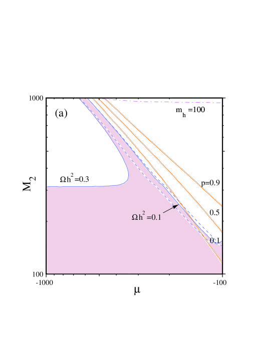
As discussed in section 4, one can make a further reduction in the number of parameters by setting all of the soft scalar masses equal at the GUT scale, thereby considering the CMSSM. For a given value of $\tan\beta$, the parameter space is best described in terms of the common gaugino masses $m_{1/2}$ and scalar masses $m_{0}$ at the GUT scale. In Figure 12 [35], this parameter space is shown for $\tan\beta=2$. The light shaded region corresponds to the portion of parameter space where the relic density $\Omega_{\chi}h^{2}$ is between 0.1 and 0.3. The darker shaded region corresponds to the parameters where the LSP is not a neutralino but rather a ${{\tilde{\tau}}}_{R}$. In the $m_{0}-m_{1/2}$ plane, the upper limit to $m_{0}$ is due to the upper limit $\Omega_{\chi}h^{2}<0.3$. For larger $m_{0}$, the large sfermion masses suppress the annihilation cross-section which is then too small to bring the relic density down to acceptable levels. In this region, the LSP is mostly ${\widetilde{B}}$, and the value of $\mu$ can not be adjusted to make the LSP a Higgsino which would allow an enhanced annihilation particularly at large $m_{0}$. The cosmologically interesting region at the left of the figure is rather jagged, due to the appearance of pole effects. There, the LSP can annihilate through s-channel $Z$ and $h$ (the light Higgs) exchange, thereby allowing a very large value of $m_{0}$. Because the $\Omega_{\chi}h^{2}=0.3$ contour runs into the ${{\tilde{\tau}}}_{R}$-LSP region at a given value of $m_{1/2}$, it was thought [32] that this point corresponded to an upper limit to the LSP mass (since $m_{{\tilde{B}}}$ is approximately 0.4 $m_{1/2}$. As we will see, this limit has been extended due to co-annihilations of the ${{\widetilde{B}}}$ and ${{\tilde{\tau}}}_{R}$ [110].

Figure 12: Region in the $m_{1/2}$–$m_{0}$ plane where $0.1\leq\Omega h^{2}\leq 0.3$ [35]. Masses are in GeV.

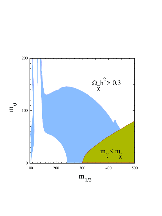
The $m_{1/2}-m_{0}$ parameter space is further constrained by the recent runs at LEP. The negative results of LEP 1 searches for $Z^{0}\rightarrow\chi^{+}\chi^{-}$ and $Z^{0}\rightarrow\chi\chi^{\prime}$ (where $\chi^{\prime}$ denotes a generic heavier neutralino) already established important limits on supersymmetric model parameters, but left open the possibility that the lightest neutralino might be massless [94]. Subsequently, the data from higher-energy LEP runs, based on chargino and neutralino pair production, complemented LEP 1 data and excluded the possibility of a massless neutralino, at least if the input gaugino masses $M_{\alpha}$ were assumed to be universal [111, 91].

In Figure 13 [112], the constraints imposed by the LEP chargino and neutralino and slepton searches [111, 96] (hatched region) at LEP 2 are shown. The hatched regions correspond to the limits in the MSSM. The thick curve to the right of this region, corresponds to the slightly more restrictive bound due to the assumption of universal Higgs masses at the GUT scale (CMSSM). The distinction between these two cases is more apparent at other values of $\tan\beta$ [91, 112]. The bounds shown here correspond to the run at LEP at 172 GeV center of mass energy. The D0 limit on the gluino mass [113] is also shown (dotted line). Of particular importance are the bounds on supersymmetric Higgs production, for which we consider both the $e^{+}e^{-}\rightarrow hZ$ and $e^{+}e^{-}\rightarrow hA$ reactions. The regions bounded by the lack of Higgs events are labeled nUHM corresponding to the MSSM (non-Universal Higgs Mass) and UHM corresponding to the UHM. Once again, the limits plotted in this figure (13) correspond to the 172 GeV run and have been greatly improved since. In this case the improvement in the bound when restricting the value of $\mu$ to take its CMSSM value is clear. At lower $\tan\beta$, the constraint curve moves quickly to the left, i.e., to higher values of $m_{1/2}$ [112].

Figure 13: The domains of the $m_{1/2}$–$m_{0}$ plane (masses in GeV) that are excluded by the LEP 2 chargino and selectron searches, both without (hatched) and with the assumption of Higgs scalar-mass universality for $\mu<0$ and $\tan\beta=2$ [112]. Also displayed are the domains that are excluded by Higgs searches (solid lines) with and without the assumption of universal scalar masses for Higgs bosons (UHM). The region marked theory is excluded cosmologically because $m_{{\tilde{\tau}}_{R}}<m_{\chi}$. The domains that have relic neutralino densities in the favored range with (dark) and without (light shaded) the scalar-mass universality assumption.

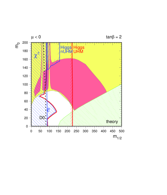
The region of the $m_{1/2}-m_{0}$ plane in which $0.1<\Omega_{\chi}h^{2}<0.3$ for some experimentally allowed value of $\mu<0$ is light-shaded in Figure 13, and the region of the plane in which $0.1<\Omega_{\chi}h^{2}<0.3$ for $\mu$ determined by the CMSSM constraint on the scalar masses is shown dark-shaded. The MSSM region extends to large values of $m_{0}$ since $\mu$ can be adjusted to take low values so the the LSP is Higgsino like and the relic density becomes insensitive to the sfermion masses.

As one can see from Figure 13, the combined bounds from the chargino and slepton searches, provide a lower bound to $m_{1/2}$ which can be translated into a bound on the neutralino mass. In the region of interest, we have the approximate relation that $m_{\chi}\approx 0.4m_{1/2}$.

Figure 14: The light-shaded area is the cosmologically preferred region with $0.1\leq\Omega h^{2}\leq 0.3$. The light dashed lines show the location of the cosmologically preferred region if one ignores coannihilations with the light sleptons. In the dark shaded regions in the bottom right of each panel, the LSP is the ${\tilde{\tau}}_{R}$, leading to an unacceptable abundance of charged dark matter. Also shown are the isomass contours $m_{\chi^{\pm}}=95$ GeV and $m_{h}=95,100,105,110$ GeV, as well as an indication of the slepton bound from LEP [115]. These figures are adapted from those in [110].

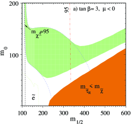
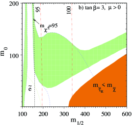
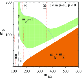
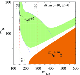
Ultimately, the Higgs mass bound alone does not provide an independent bound on $m_{1/2}$. The reason is that the Higgs constraint curves bend to the left at large $m_{0}$, where large sfermion masses lead to greater positive radiative corrections to the Higgs mass, and the Higgs curve strikes the chargino bound at sufficiently large $m_{0}$. However, when combined with cosmological limit on the relic density, a stronger constraint can be found. Recall that at large $m_{0}$, the cosmological bound is satisfied by lowering $\mu$. At certain values of $\tan\beta$ and $m_{1/2}$, one can not lower $\mu$ and remain consistent with the relic density limit and the Higgs mass limit. This is seen in Figure 13 by the short horizontal extension of the nUHM Higgs curve. At lower values of $\tan\beta$ this extension is lengthened. In the UHM case, once again the UHM Higgs curve bends to the right at large $m_{0}$. However, cosmology excludes the large $m_{0}$ region in the CMSSM (CMSSM and UHM are treated synonymously here). In this case the mass bound on $m_{1/2}$ or $m_{\chi}$ is much stronger.

The results from the 172 GeV run at LEP provided a bound on the chargino mass of $m_{\chi^{\pm}}>86$ GeV and corresponding bound on the neutralino mass of $m_{\chi}\mathrel{\raise 1.29167pt\hbox{$>$\kern-7.5pt\lower 4.30554pt\hbox{$\sim$}}}40$ GeV [112]. As noted above, the UHM Higgs mass bound becomes very strong at low $\tan\beta$. In fact, for $\tan\beta<1.7$, the UHM Higgs curve moves so far to the left so as to exclude the entire dark shaded region required by cosmology. Subsequent to the 183 GeV run at LEP [114], the chargino mass bound was pushed to $m_{\chi^{\pm}}>91$ GeV, and a Higgs mass bound was established to be $m_{h}\mathrel{\raise 1.29167pt\hbox{$>$\kern-7.5pt\lower 4.30554pt\hbox{$\sim$}}}86$ GeV for $\tan\beta\mathrel{\raise 1.29167pt\hbox{$<$\kern-7.5pt\lower 4.30554pt\hbox{$\sim$}}}3$, and $m_{h}\mathrel{\raise 1.29167pt\hbox{$>$\kern-7.5pt\lower 4.30554pt\hbox{$\sim$}}}76$ GeV for $\tan\beta\mathrel{\raise 1.29167pt\hbox{$>$\kern-7.5pt\lower 4.30554pt\hbox{$\sim$}}}3$. These limits were further improved by the 189 GeV run, so that at the kinematic limit the chargino mass bound is $m_{\chi^{\pm}}\mathrel{\raise 1.29167pt\hbox{$>$\kern-7.5pt\lower 4.30554pt\hbox{$\sim$}}}95$ GeV, implying that $m_{1/2}\mathrel{\raise 1.29167pt\hbox{$>$\kern-7.5pt\lower 4.30554pt\hbox{$\sim$}}}110$ GeV and the neutralino mass limit becomes $m_{\chi}\mathrel{\raise 1.29167pt\hbox{$>$\kern-7.5pt\lower 4.30554pt\hbox{$\sim$}}}50$ Gev. The Higgs mass bound is now (as of the 189 run) $m_{h}\mathrel{\raise 1.29167pt\hbox{$>$\kern-7.5pt\lower 4.30554pt\hbox{$\sim$}}}95$ GeV for low $\tan\beta$ [115].

Figure 15: The same as Fig. 14, for $\mu<0$, but extended to larger $m_{1/2}$. These figures are adapted from those in [110].

Figure 16: As in 14 for $\tan\beta=2,2.5$, and 3, for both $\mu>0$ and $\mu<0$. Higgs mass contours of 86, 95, and 96 GeV, are displayed to show the dependence on $\tan\beta$. I thank Toby Falk for providing these figures.

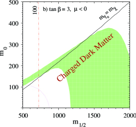
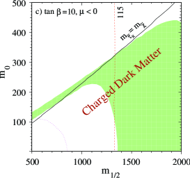
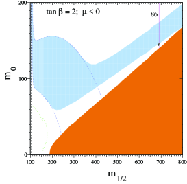
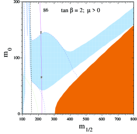
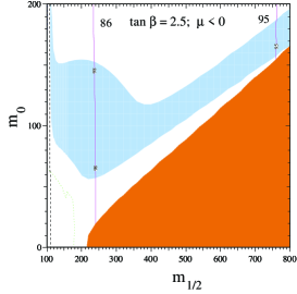
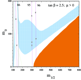
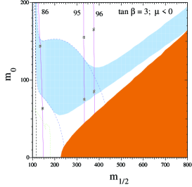
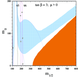
In the MSSM, in the region of the $M_{2}$-$\mu$ plane, where $H_{(12)}$ is the LSP (that is, at large $\mu$ and very large $M_{2}$), the next lightest neutralino or NLSP, is the $H_{[12]}$ state and the two are nearly degenerate with masses close to $\mu$. In this case, additional annihilation channels (or co-annihilation) which involve both a $H_{(12)}$ and a $H_{[12]}$ in the initial state become important [106, 107]. The enhanced annihilation of Higgsinos lowers the relic density substantially and virtually eliminates the Higgsino as a viable dark matter candidate. In the CMSSM, co-annihilation is also important, now at large values of $m_{1/2}$ [110]. Recall, that previously we discussed a possible upper limit to the mass of the neutralino in the CMSSM, where the cosmologically allowed region of Figure 12 runs into the region where the ${\tilde{\tau}}_{R}$ is the LSP. Along the boundary of this region, the neutralino ${\widetilde{B}}$, and the ${\tilde{\tau}}_{R}$ are degenerate. Therefore close to this boundary, new co-annihilation channels involving both ${\widetilde{B}}$ and ${\tilde{\tau}}_{R}$ (as well as the other right-handed sleptons which are also close in mass) in the initial state become important. As in the MSSM, the co-annihilations reduce the relic density and as can be seen in Figures 14 the upper limit to the neutralino is greatly relaxed [110]. As one can plainly see, the cosmologically allowed region is bent way from the ${\tilde{\tau}}_{R}$-LSP region extending to higher values of $m_{1/2}$. Also shown in this set of figures are the iso-mass contours for charginos, sleptons and Higgses, so that the LEP limits discussed above can be applied. In these figures, one can see the sensitivity of the Higgs mass with $\tan\beta$.

Despite the importance of the coannihilation, there is still an upper limit to the neutralino mass. If we look at an extended version of Figures 14, as shown in Figures 15, we see that eventually, the cosmologically allowed region intersects the ${\tilde{\tau}}_{R}$-LSP region. The new upper limit occurs at $m_{1/2}\approx 1450$ GeV, implying that $m_{\chi}\mathrel{\raise 1.29167pt\hbox{$<$\kern-7.5pt\lower 4.30554pt\hbox{$\sim$}}}600$ GeV.

As noted above, the Higgs mass bounds can be used to exclude low values of $\tan\beta$. However, when co-annihilations are included, the limits on $\tan\beta$ is weakened. In the $m_{1/2}-m_{0}$ plane, the Higgs iso-mass contour appears nearly vertical for low values of $m_{0}$. A given contour is highly dependent on $\tan\beta$, and moves to the right quickly as $\tan\beta$ decreases. This behavior is demonstrated in the series of Figures 16, which show the positions of the Higgs mass contours for $\tan\beta=2,2.5,$ and 3, for both positive and negative $\mu$. If we concentrate, on the 95 GeV contour, we see that at $\tan\beta=3$, the bulk of the cosmological region is allowed. At $\tan\beta=2.5$, much of the bulk is excluded, though the trunck region is allowed. At the lower value of $\tan\beta=2$, the 95 GeV contour is off the scale of this figure. A thorough examination [110] yields a limit $\tan\beta>2.2$ for $\mu<0$. For positive $\mu$, the results are qualitatively similar. The Higgs mass contours are farther to the left (relative to the negative $\mu$ case), and the limit on $\tan\beta$ is weaker. Nevertheless the limit is $\tan\beta>1.8$ for $\mu>0$.

As the runs at LEP are winding down, the prospects for improving the current limits or more importantly discovering supersymmetry are diminishing. Further progress will occur in the future with Run II at the Tevetron at ultimately and the LHC. Currently, while we have strong and interesting limits on the MSSM and CMSSM parameter space for LEP, much of the phenomenological and cosmological parameter space remains viable.

Acknowledgments I would like to thank B. Campbell, S. Davidson, J. Ellis, K. Enqvist, T. Falk, M.K. Gaillard, G. Ganis, J. Hagelin, K. Kainulainen, R. Madden, J. McDonald, H. Murayama, D.V. Nanopoulos, S.J. Rey, M. Schmitt, M. Srednicki, K. Tamvakis, R. Watkins for many enjoyable collaborations which have been summarized in these lectures. I would also like to thank J. Ellis, T. Falk, S. Lee, and M. Voloshin for assistance in the preparation of these lecture notes. This work was supported in part by DOE grant DE-FG02-94ER40823 at Minnesota.